che-101: approaches to chemical engineering...

Tutorial VIII: Excel Basics Last updated 4/12/06 by G.G. Botte

1

Department of Chemical Engineering ChE-101: Approaches to Chemical Engineering Problem Solving

Excel Tutorial VIII EXCEL Basics (last updated 4/12/06 by GGB) Objectives: These tutorials are designed to show the introductory elements for any of the topics discussed. In almost all cases there are other ways to accomplish the same objective, or higher level features that can be added to the commands below. ______________________________________________________________________________ The following topics are covered in this tutorial; What is EXCEL? Starting EXCEL Saving a file Exiting EXCEL Online Help Doing Calculations with EXCEL Labeling a sheet Formatting text Creating Values with an Equation Number Display Formats Different formatting Creating borders with EXCEL Plotting in EXCEL Useful toolbars Calculate minimum, maximum, average Using values from different sheets for a calculation Proposed Problem ===================================================================== What is EXCEL? EXCEL is a windows program oriented that allows you to: compute different calculations (predefined functions or operations defined by the user), plot, construct tables, organize information, draw, etc. ===================================================================== Starting EXCEL Double click on the EXCEL icon. The EXCEL worksheet will appear. Each worksheet has different calculation sheets. Different tool bars will show up in the menu according to the configuration shown by the user. All the formatting options available in Microsoft Word are also available in EXCEL. The worksheet has different cells each cell has a letter and a number associated with it. The letter indicates the column name and the number indicates the row number. See figure shown below. =====================================================================

2

Saving a File To save a file click on the File drop up window and select “save as” as shown below

Worksheet

Row numberColumn label

Cell K4

Formatting toolbar

Drawing toolbar

Worksheet

Row numberColumn label

Cell K4

Formatting toolbar

Drawing toolbar

Type your file nameBy default it will be

saved as an Excel workbook (DO NOT CHANGE THIS) After choosing file

name press the save button

Type your file nameBy default it will be

saved as an Excel workbook (DO NOT CHANGE THIS) After choosing file

name press the save buttonThe name of your

file will show up in the window

The name of your file will show up in the window


3

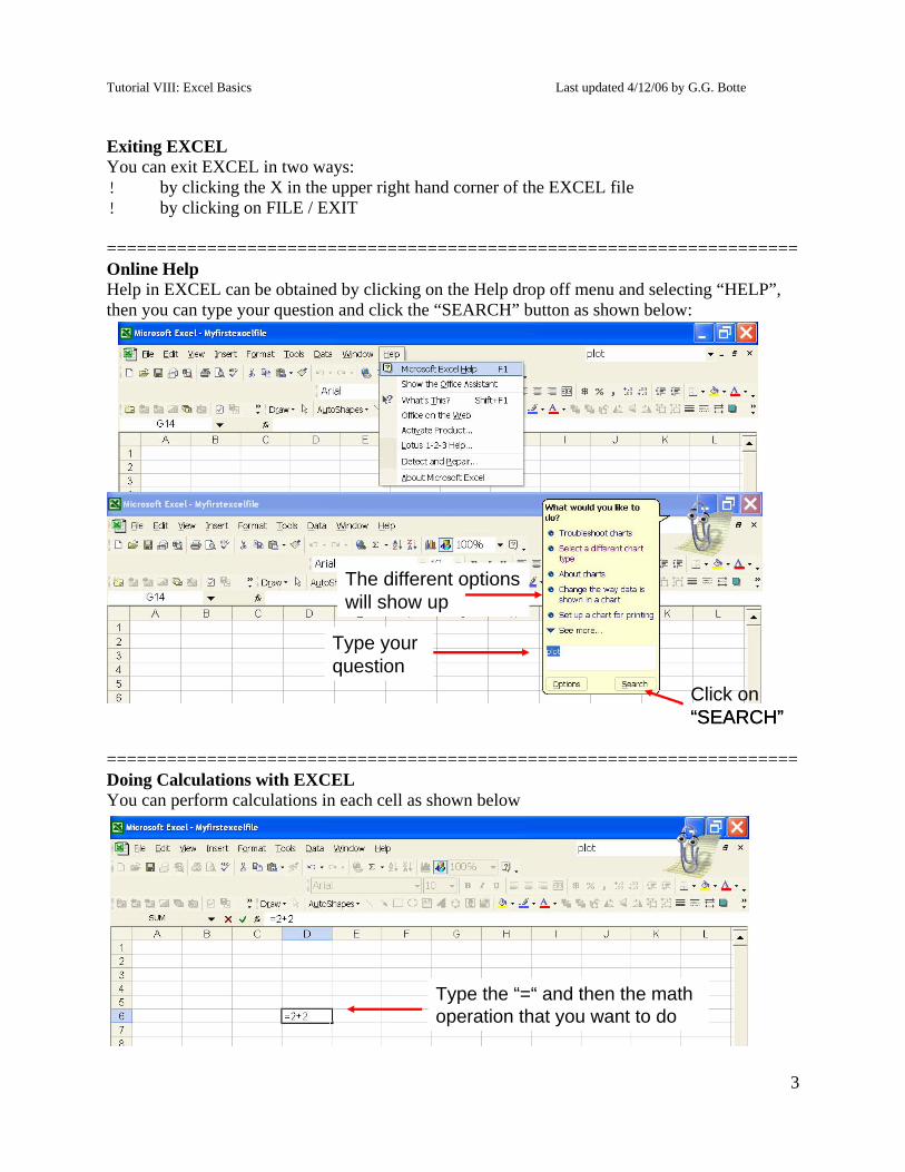
Exiting EXCEL You can exit EXCEL in two ways: ! by clicking the X in the upper right hand corner of the EXCEL file ! by clicking on FILE / EXIT ===================================================================== Online Help Help in EXCEL can be obtained by clicking on the Help drop off menu and selecting “HELP”, then you can type your question and click the “SEARCH” button as shown below: ===================================================================== Doing Calculations with EXCEL You can perform calculations in each cell as shown below

Type your question

Click on “SEARCH”

The different options will show up

Type your question

Click on “SEARCH”

The different options will show up

Type the “=“ and then the math operation that you want to doType the “=“ and then the math operation that you want to do

4

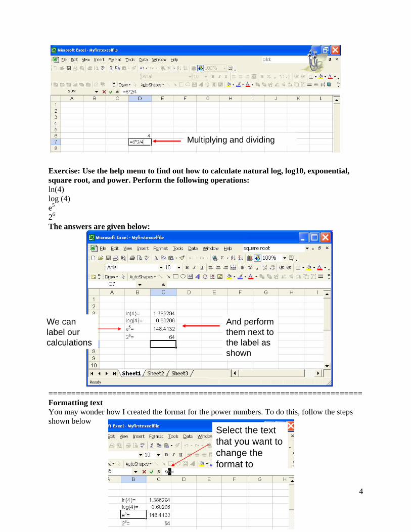
Exercise: Use the help menu to find out how to calculate natural log, log10, exponential, square root, and power. Perform the following operations: ln(4) log (4) e5

26

The answers are given below: ===================================================================== Formatting text You may wonder how I created the format for the power numbers. To do this, follow the steps shown below

Multiplying and dividingMultiplying and dividing

We can label our calculations

And perform them next to the label as shown

We can label our calculations

And perform them next to the label as shown

Select the text that you want to change the format to

Select the text that you want to change the format to


5

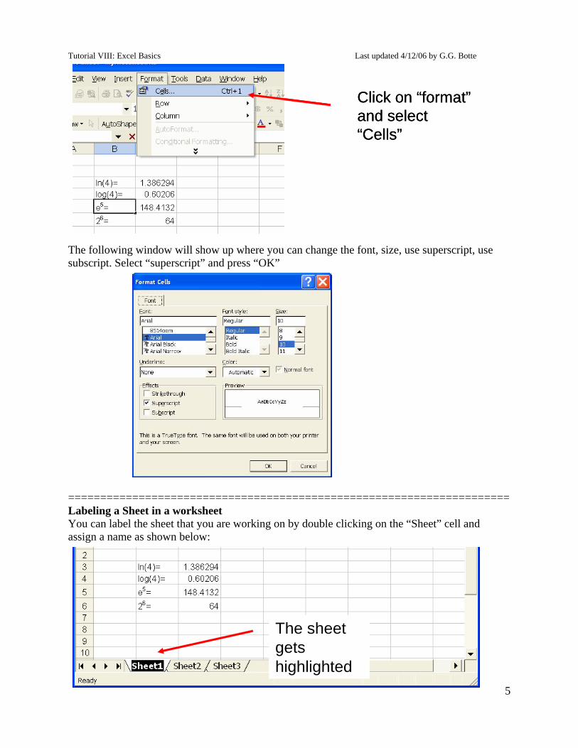
The following window will show up where you can change the font, size, use superscript, use subscript. Select “superscript” and press “OK” ===================================================================== Labeling a Sheet in a worksheet You can label the sheet that you are working on by double clicking on the “Sheet” cell and assign a name as shown below:

The sheet gets highlighted

The sheet gets highlighted

Click on “format” and select “Cells”

Click on “format” and select “Cells”

6

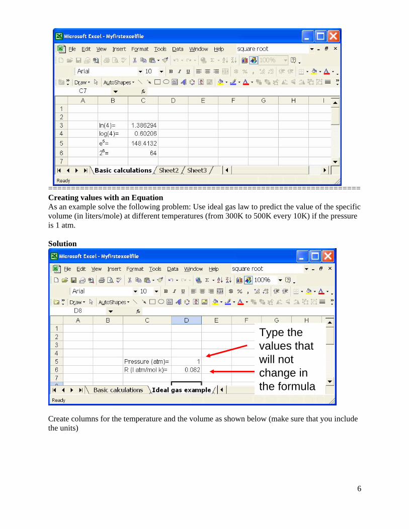
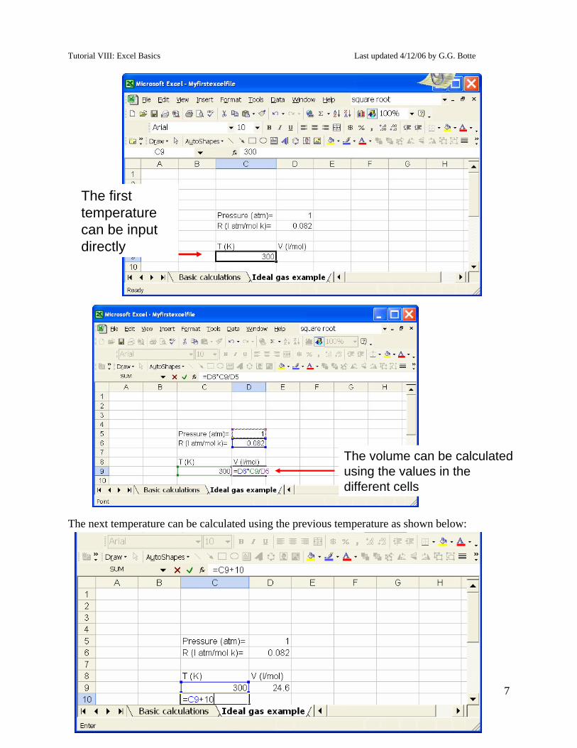
===================================================================== Creating values with an Equation As an example solve the following problem: Use ideal gas law to predict the value of the specific volume (in liters/mole) at different temperatures (from 300K to 500K every 10K) if the pressure is 1 atm. Solution Create columns for the temperature and the volume as shown below (make sure that you include the units)

Type the values that will not change in the formula

Type the values that will not change in the formula


7

The next temperature can be calculated using the previous temperature as shown below:

The first temperature can be input directly

The first temperature can be input directly

The volume can be calculated using the values in the different cells

The volume can be calculated using the values in the different cells

8

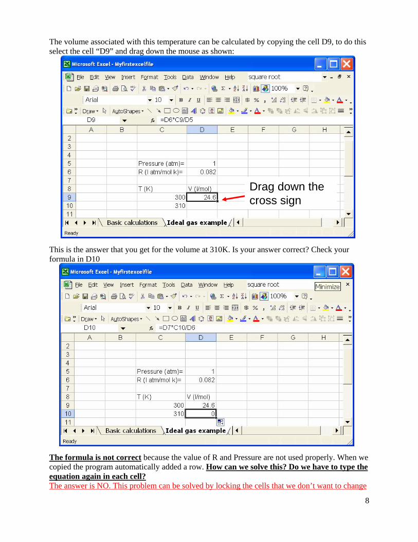
The volume associated with this temperature can be calculated by copying the cell D9, to do this select the cell “D9” and drag down the mouse as shown: This is the answer that you get for the volume at 310K. Is your answer correct? Check your formula in D10 The formula is not correct because the value of R and Pressure are not used properly. When we copied the program automatically added a row. How can we solve this? Do we have to type the equation again in each cell? The answer is NO. This problem can be solved by locking the cells that we don’t want to change

Drag down the cross signDrag down the cross sign


9

during a calculation. For example in this case neither pressure nor the R changes in each calculation. Therefore, we need to correct the equation used in cell D9 by locking the cells in R and pressure using the function “F4” as shown below: Now we can copy the formula to the next cell D10 and we should get the correct answer:

By clicking “F4” two $ signs appeared. We can also type the $ signs without using “F4” The first $ sign indicates that the column will be locked and the second $ indicates that the row will be locked

By clicking “F4” two $ signs appeared. We can also type the $ signs without using “F4” The first $ sign indicates that the column will be locked and the second $ indicates that the row will be locked

The formula is correctThe formula is correct

10

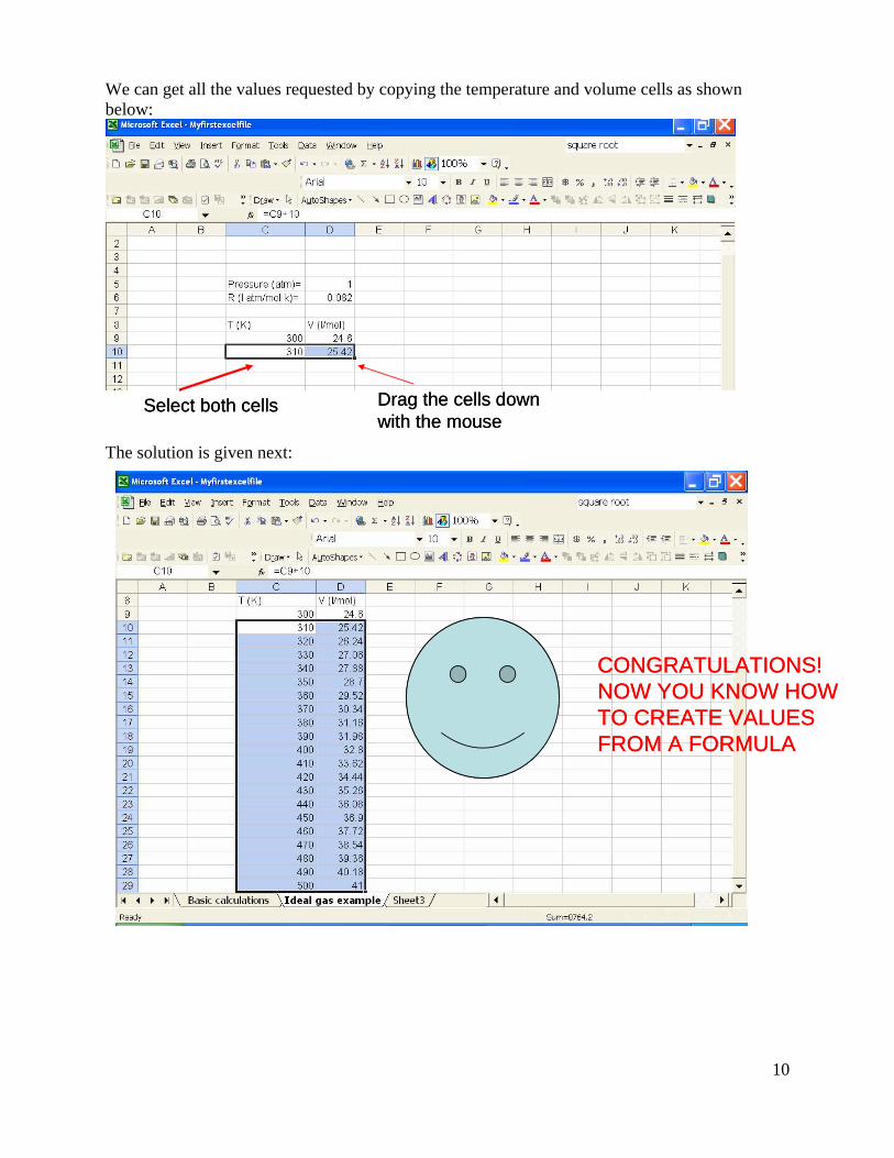
We can get all the values requested by copying the temperature and volume cells as shown below: The solution is given next:

Select both cells Drag the cells down with the mouse

Select both cells Drag the cells down with the mouse

CONGRATULATIONS! NOW YOU KNOW HOW TO CREATE VALUES FROM A FORMULA

CONGRATULATIONS! NOW YOU KNOW HOW TO CREATE VALUES FROM A FORMULA


11

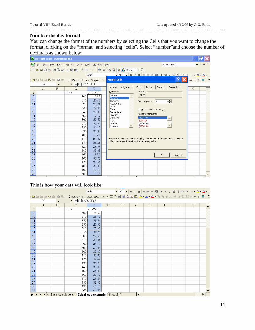
===================================================================== Number display format You can change the format of the numbers by selecting the Cells that you want to change the format, clicking on the “format” and selecting “cells”. Select “number”and choose the number of decimals as shown below: This is how your data will look like:

12

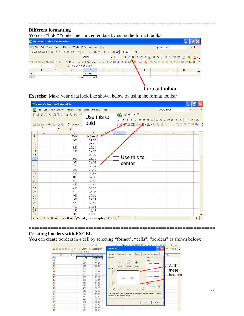
===================================================================== Different formatting You can “bold” “underline” or center data by using the format toolbar Exercise: Make your data look like shown below by using the format toolbar ===================================================================== Creating borders with EXCEL You can create borders in a cell by selecting “format”, “cells”, “borders” as shown below:

Format toolbarFormat toolbar

Use this to center

Use this to bold

Use this to center

Use this to bold

Add these borders

Add these borders


13

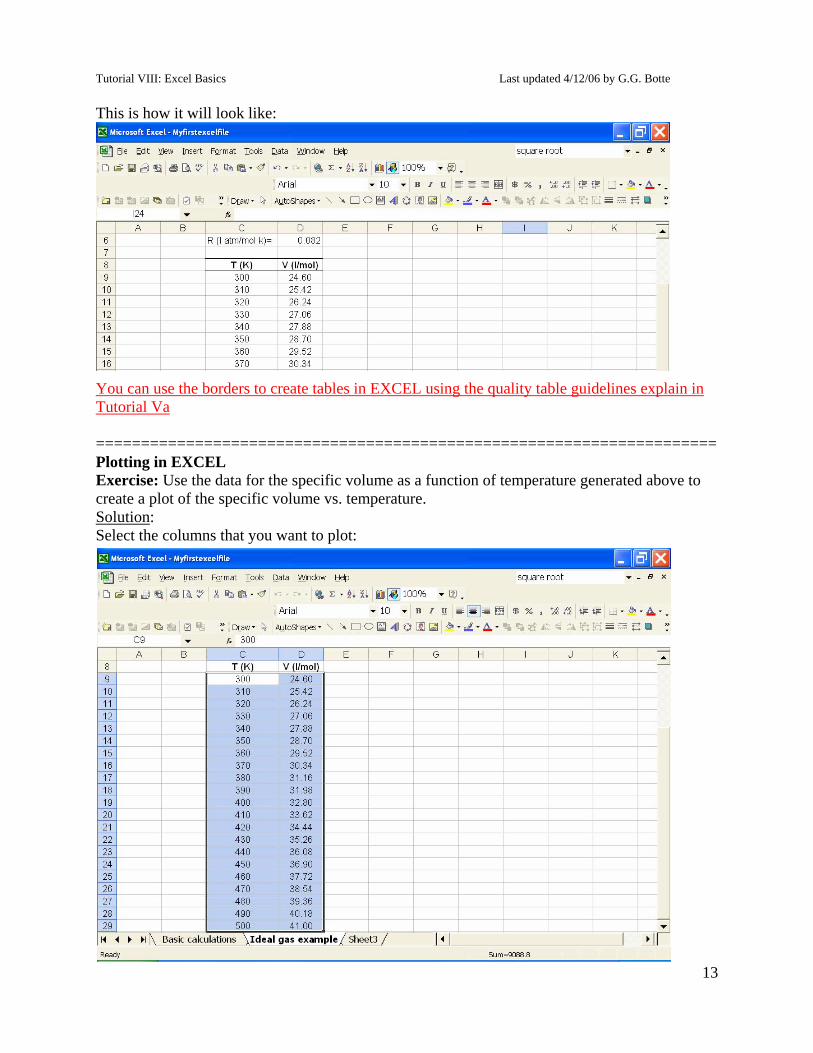
This is how it will look like: You can use the borders to create tables in EXCEL using the quality table guidelines explain in Tutorial Va ===================================================================== Plotting in EXCEL Exercise: Use the data for the specific volume as a function of temperature generated above to create a plot of the specific volume vs. temperature. Solution: Select the columns that you want to plot:

14

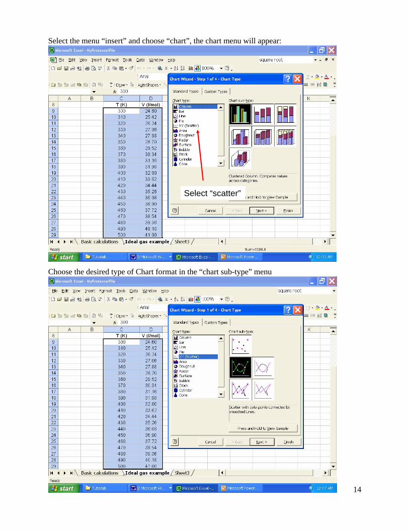
Select the menu “insert” and choose “chart”, the chart menu will appear: Choose the desired type of Chart format in the “chart sub-type” menu

Select “scatter”Select “scatter”


15

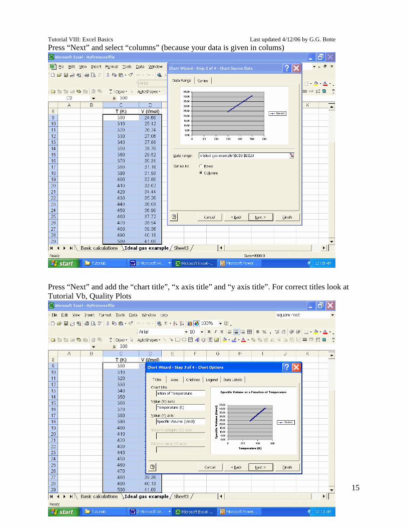
Press “Next” and select “columns” (because your data is given in colums) Press “Next” and add the “chart title”, “x axis title” and “y axis title”. For correct titles look at Tutorial Vb, Quality Plots

16

Click “Next” and choose “Chart Location” “As new Sheet” This is how your graph will look like. Now you can modify it to follow the guidelines explain in Tutorial Vb (Quality Plots). For example: Eliminate gridlines, erase grey area

Give title

Eliminate grey area and gridlines

Give title

Eliminate grey area and gridlines


17

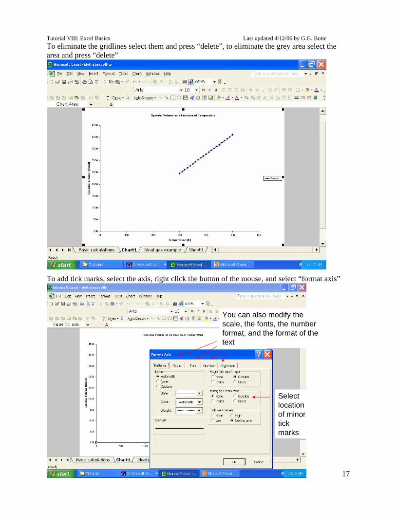
To eliminate the gridlines select them and press “delete”, to eliminate the grey area select the area and press “delete” To add tick marks, select the axis, right click the button of the mouse, and select “format axis”

Select location of minor tick marks

You can also modify the scale, the fonts, the number format, and the format of the text

Select location of minor tick marks

You can also modify the scale, the fonts, the number format, and the format of the text

18

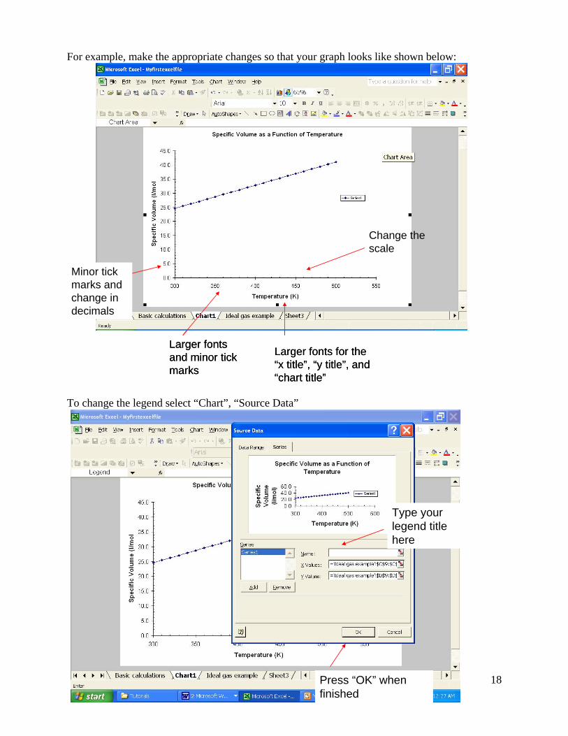
For example, make the appropriate changes so that your graph looks like shown below: To change the legend select “Chart”, “Source Data”

Change the scale

Larger fonts and minor tick marks

Larger fonts for the “x title”, “y title”, and “chart title”

Minor tick marks and change in decimals

Change the scale

Larger fonts and minor tick marks

Larger fonts for the “x title”, “y title”, and “chart title”

Minor tick marks and change in decimals

Type your legend title here

Press “OK” when finished


19

You can change the position of the legend by selecting the legend box and dragging it with the mouse (left button) You can change the format of the data by selecting the data, right click on the mouse button and press “Format Data Series”

20

Then you can make different selections as shown below: ===================================================================== Useful toolbars You can choose what toolbars to see in your file by clicking on “View” and selecting the different toolbars

Different toolbars that will show up if the user wants to see them

Different toolbars that will show up if the user wants to see them


21

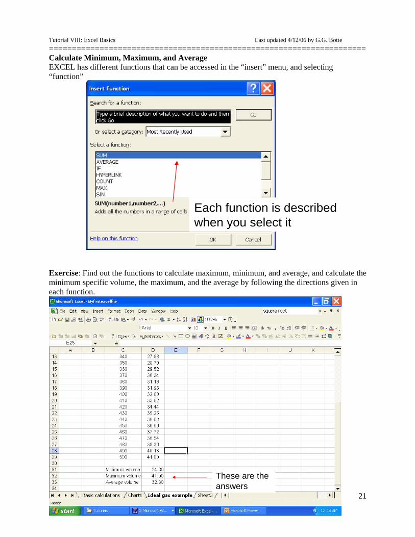
===================================================================== Calculate Minimum, Maximum, and Average EXCEL has different functions that can be accessed in the “insert” menu, and selecting “function” Exercise: Find out the functions to calculate maximum, minimum, and average, and calculate the minimum specific volume, the maximum, and the average by following the directions given in each function.

Each function is described when you select itEach function is described when you select it

These are the answersThese are the answers

22

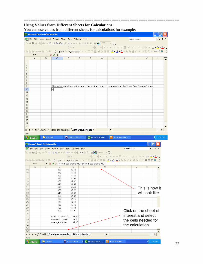
===================================================================== Using Values from Different Sheets for Calculations You can use values from different sheets for calculations for example:

Click on the sheet of interest and select the cells needed for the calculation

This is how it will look like

Click on the sheet of interest and select the cells needed for the calculation

This is how it will look like


23

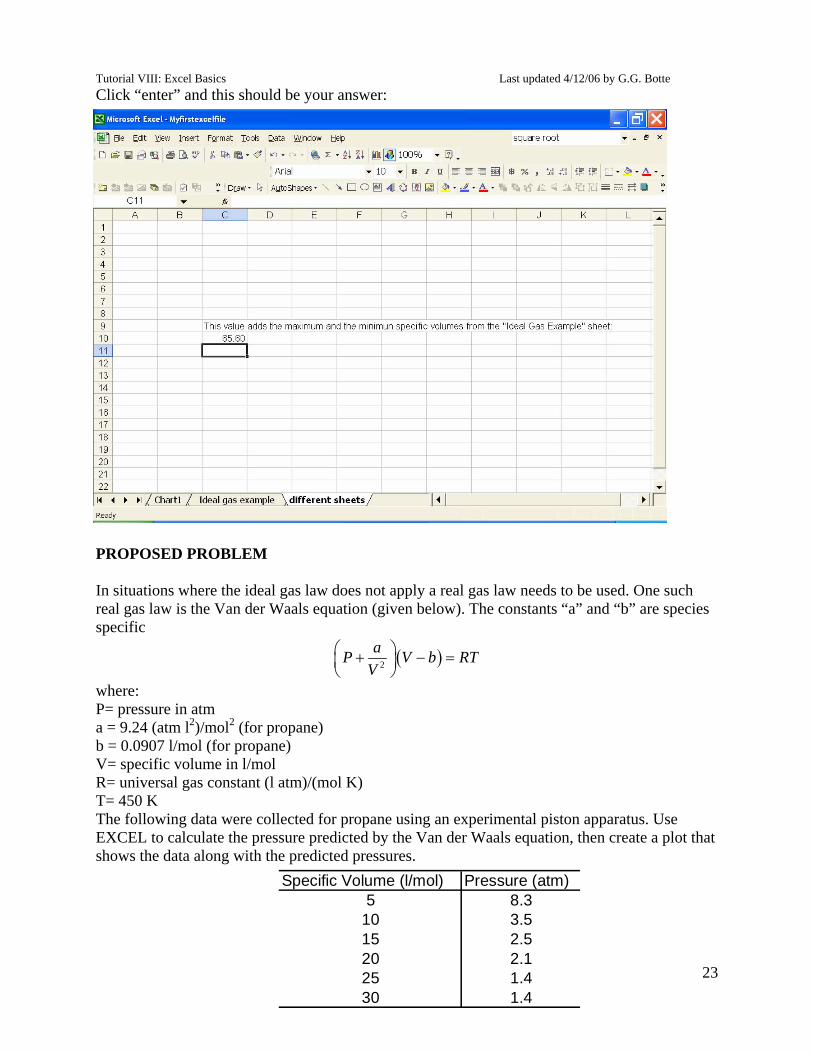
Click “enter” and this should be your answer: PROPOSED PROBLEM In situations where the ideal gas law does not apply a real gas law needs to be used. One such real gas law is the Van der Waals equation (given below). The constants “a” and “b” are species specific

( )2

aP V b RTV

⎛ ⎞+ − =⎜ ⎟⎝ ⎠

where: P= pressure in atm a = 9.24 (atm l2)/mol2 (for propane) b = 0.0907 l/mol (for propane) V= specific volume in l/mol R= universal gas constant (l atm)/(mol K) T= 450 K The following data were collected for propane using an experimental piston apparatus. Use EXCEL to calculate the pressure predicted by the Van der Waals equation, then create a plot that shows the data along with the predicted pressures.

Specific Volume (l/mol) Pressure (atm)5 8.3

10 3.515 2.520 2.125 1.430 1.4

che-101: approaches to chemical engineering...

Documents