checking assumptions 1 copyright © 2005 brooks/cole, a division of thomson learning, inc. chapter 6...

Checking AssumptionsChecking Assumptions 11Copyright © 2005 Brooks/Cole, a division of Thomson Learning, Inc.Copyright © 2005 Brooks/Cole, a division of Thomson Learning, Inc.

Chapter 6Chapter 6Assessing the Assumptions of Assessing the Assumptions of

the Regression Modelthe Regression Model

Terry Dielman Terry Dielman

Applied Regression AnalysisApplied Regression Analysisfor Business and Economicsfor Business and Economics


6.1 Introduction6.1 Introduction

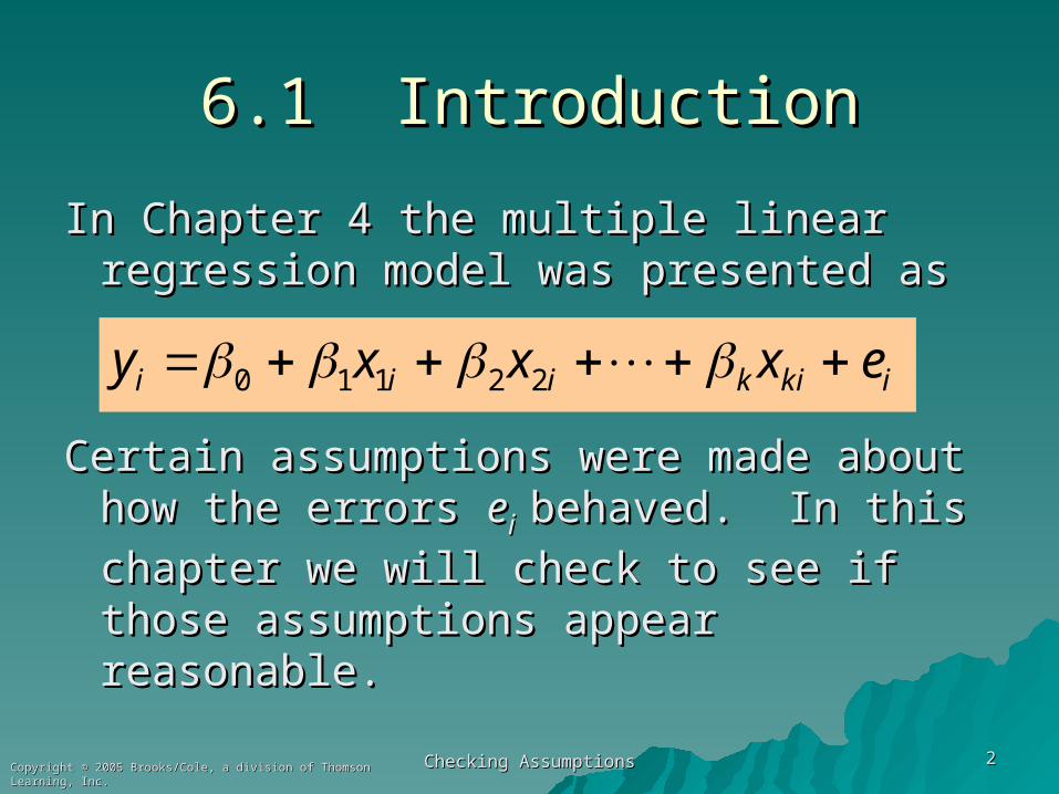
In Chapter 4 the multiple linear In Chapter 4 the multiple linear regression model was presented asregression model was presented as

Certain assumptions were made about Certain assumptions were made about how the errors how the errors eei i behaved. In this behaved. In this

chapter we will check to see if those chapter we will check to see if those assumptions appear reasonable.assumptions appear reasonable.

ikikiii exxxy 22110


6.2 Assumptions of the Multiple Linear Regression Model6.2 Assumptions of the Multiple Linear Regression Model

a.a. We expect the average disturbance We expect the average disturbance eeii to be zero so the regression line to be zero so the regression line passes through the average value passes through the average value of Y.of Y.

b.b. The disturbances have constant The disturbances have constant variance variance ee

22..c.c. The disturbances are normally The disturbances are normally

distributed.distributed.d.d. The disturbances are independent.The disturbances are independent.


6.3 The Regression Residuals6.3 The Regression Residuals

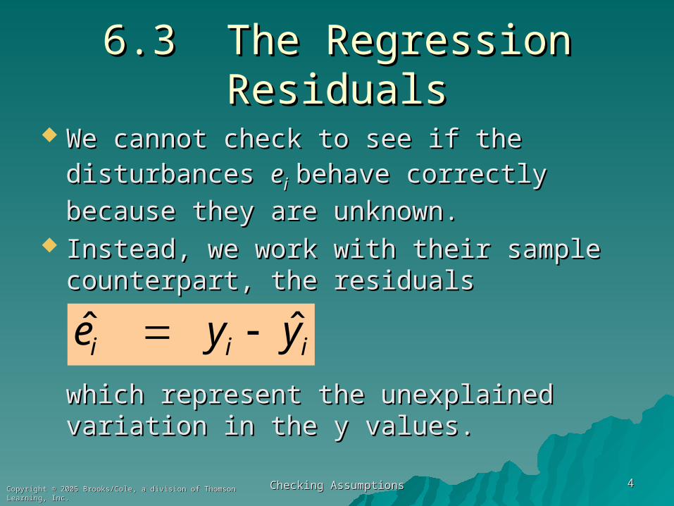
We cannot check to see if the disturbances We cannot check to see if the disturbances eeii behave correctly because they are behave correctly because they are

unknown.unknown. Instead, we work with their sample Instead, we work with their sample

counterpart, the residualscounterpart, the residuals

which represent the unexplained variation which represent the unexplained variation in the y values.in the y values.

iii yye ˆˆ


PropertiesPropertiesProperty 1: Property 1: They will always average 0 They will always average 0

because the least squares estimation because the least squares estimation procedure makes that happen.procedure makes that happen.

Property 2: Property 2: If assumptions a, b and d of If assumptions a, b and d of Section 6.2 are true then the residuals Section 6.2 are true then the residuals should be randomly distributed around should be randomly distributed around their mean of 0. There should be no their mean of 0. There should be no systematic pattern in a residual plot.systematic pattern in a residual plot.

Property 3: Property 3: If assumptions a through d hold, If assumptions a through d hold, the residuals should look like a random the residuals should look like a random sample from a normal distribution.sample from a normal distribution.


Suggested Residual PlotsSuggested Residual Plots

1.1. Plot the residuals versus each Plot the residuals versus each explanatory variable.explanatory variable.

2.2. Plot the residuals versus the Plot the residuals versus the predicted values.predicted values.

3.3. For data collected over time or in For data collected over time or in any other sequence, plot the any other sequence, plot the residuals in that sequence.residuals in that sequence.

In addition, a histogram and box plot In addition, a histogram and box plot are useful for assessing normality. are useful for assessing normality.


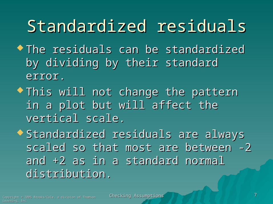
Standardized residualsStandardized residuals The residuals can be standardized by The residuals can be standardized by

dividing by their standard error.dividing by their standard error. This will not change the pattern in a This will not change the pattern in a

plot but will affect the vertical scale.plot but will affect the vertical scale. Standardized residuals are always Standardized residuals are always

scaled so that most are between -2 scaled so that most are between -2 and +2 as in a standard normal and +2 as in a standard normal distribution.distribution.


A plot meeting property 2A plot meeting property 2

11010510095

3

2

1

0

-1

-2

X

Res

a. mean of 0 b. Same scatter d. No pattern with X


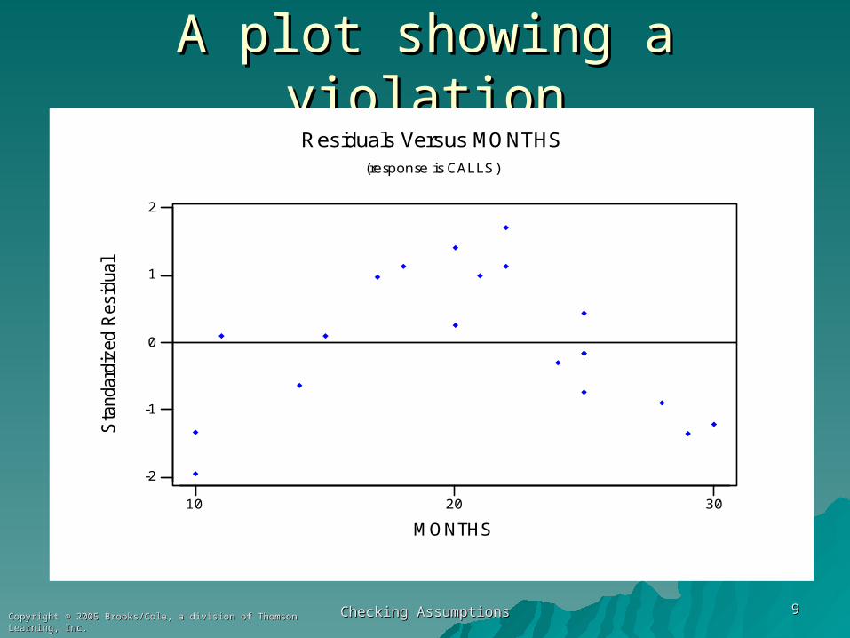
A plot showing a violationA plot showing a violation

302010

2

1

0

-1

-2

MONTHS

Sta

ndar

dize

d R

esid

ual

Residuals Versus MONTHS(response is CALLS)


6.4 Checking Linearity6.4 Checking Linearity

Although sometimes we can see evidence Although sometimes we can see evidence of nonlinearity in an X-Y scatterplot, in of nonlinearity in an X-Y scatterplot, in other cases we can only see it in a plot of other cases we can only see it in a plot of the residuals versus X.the residuals versus X.

If the plot of the residuals versus an X If the plot of the residuals versus an X shows any kind of pattern, it both shows a shows any kind of pattern, it both shows a violation and a way to improve the model.violation and a way to improve the model.


Example 6.1: TelemarketingExample 6.1: Telemarketing

n = 20 telemarketing employeesn = 20 telemarketing employees

Y = average calls per day over 20 Y = average calls per day over 20 workdaysworkdays

X = Months on the jobX = Months on the job

Data set TELEMARKET6Data set TELEMARKET6


Plot of Calls versus MonthsPlot of Calls versus Months

302010

35

30

25

20

MONTHS

CA

LL

S

There is some curvature, but it is masked by the more obvious linearity.


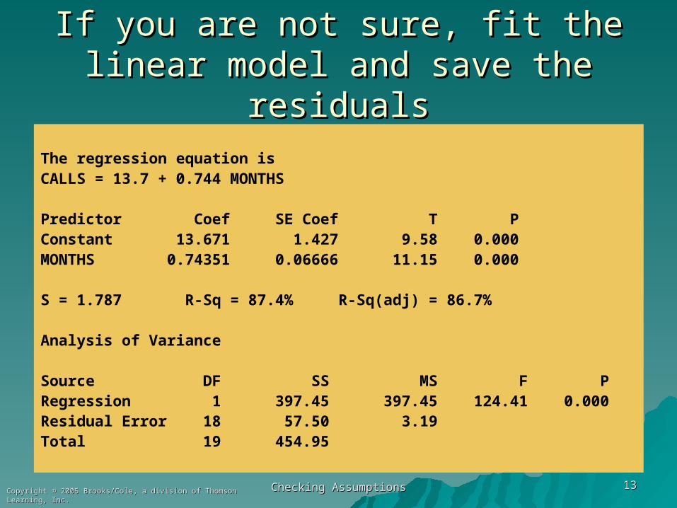
If you are not sure, fit the linear model If you are not sure, fit the linear model and save the residualsand save the residuals

The regression equation isCALLS = 13.7 + 0.744 MONTHS

Predictor Coef SE Coef T PConstant 13.671 1.427 9.58 0.000MONTHS 0.74351 0.06666 11.15 0.000

S = 1.787 R-Sq = 87.4% R-Sq(adj) = 86.7%

Analysis of Variance

Source DF SS MS F PRegression 1 397.45 397.45 124.41 0.000Residual Error 18 57.50 3.19Total 19 454.95


Residuals from modelResiduals from model

With the linearity "taken out" the curvature is more obvious


6.4.2 Tests for lack of fit6.4.2 Tests for lack of fit

The residuals contain the variation The residuals contain the variation in the sample of Y values that is not in the sample of Y values that is not explained by the Yhat equation.explained by the Yhat equation.

This variation can be attributed to This variation can be attributed to many things, including:many things, including:

• natural variation (random error)natural variation (random error)• omitted explanatory variablesomitted explanatory variables• incorrect form of modelincorrect form of model


Lack of fitLack of fit

If nonlinearity is suspected, there If nonlinearity is suspected, there are tests available for are tests available for lack of fitlack of fit..

Minitab has two versions of this Minitab has two versions of this test, one requiring there to be test, one requiring there to be repeated observations at the same repeated observations at the same X values.X values.

These are on the Options submenu These are on the Options submenu off the Regression menuoff the Regression menu


The pure error lack of fit testThe pure error lack of fit test

In the 20 observations for the In the 20 observations for the telemarketing data, there are two at telemarketing data, there are two at 10, 20 and 22 months, and four at 25 10, 20 and 22 months, and four at 25 months.months.

These replicates allow the SSE to be These replicates allow the SSE to be decomposed into two portions, "pure decomposed into two portions, "pure error" and "lack of fit".error" and "lack of fit".


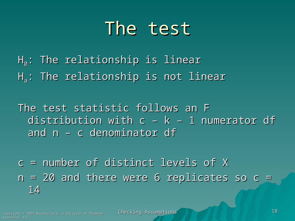
The testThe test

HH00: The relationship is linear: The relationship is linear

HHaa: The relationship is not linear: The relationship is not linear

The test statistic follows an F distribution with The test statistic follows an F distribution with c – k – 1 numerator df and n – c c – k – 1 numerator df and n – c denominator dfdenominator df

c = number of distinct levels of Xc = number of distinct levels of X

n = 20 and there were 6 replicates so c = 14n = 20 and there were 6 replicates so c = 14


Minitab's outputMinitab's outputThe regression equation isCALLS = 13.7 + 0.744 MONTHS

Predictor Coef SE Coef T PConstant 13.671 1.427 9.58 0.000MONTHS 0.74351 0.06666 11.15 0.000

S = 1.787 R-Sq = 87.4% R-Sq(adj) = 86.7%


Source DF SS MS F PRegression 1 397.45 397.45 124.41 0.000Residual Error 18 57.50 3.19 Lack of Fit 12 52.50 4.38 5.25 0.026 Pure Error 6 5.00 0.83Total 19 454.95


Test resultsTest results

At a 5% level of significance, the At a 5% level of significance, the critical value (from Fcritical value (from F12, 6 12, 6 distribution) distribution) is 4.00.is 4.00.

The computed F is 5.25 is significant (p The computed F is 5.25 is significant (p value of .026) so we conclude the value of .026) so we conclude the relationship is not linear.relationship is not linear.


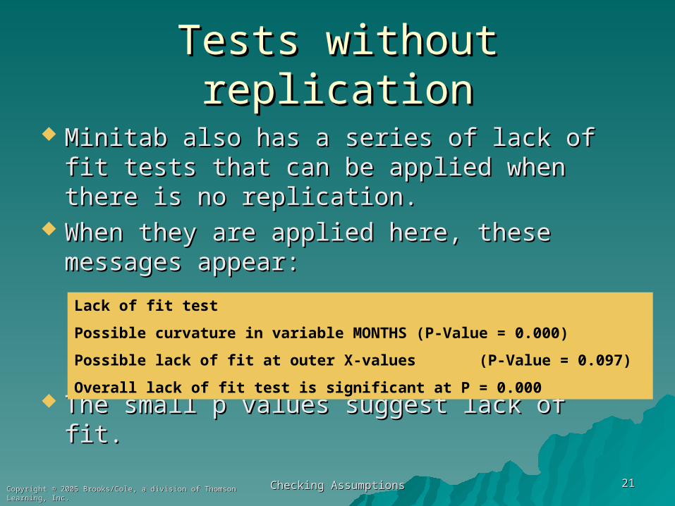
Tests without replicationTests without replication

Minitab also has a series of lack of fit tests Minitab also has a series of lack of fit tests that can be applied when there is no that can be applied when there is no replication.replication.

When they are applied here, these When they are applied here, these messages appear:messages appear:

The small p values suggest lack of fit. The small p values suggest lack of fit.

Lack of fit test

Possible curvature in variable MONTHS (P-Value = 0.000)

Possible lack of fit at outer X-values (P-Value = 0.097)

Overall lack of fit test is significant at P = 0.000


6.4.3 Corrections for nonlinearity6.4.3 Corrections for nonlinearity

If the linearity assumption is violated, If the linearity assumption is violated, the appropriate correction is not the appropriate correction is not always obvious.always obvious.

Several alternative models were Several alternative models were presented in Chapter 5.presented in Chapter 5.

In this case, it is not too hard to see In this case, it is not too hard to see that adding an Xthat adding an X22 term works well. term works well.


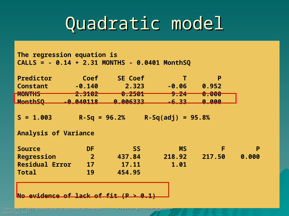
Quadratic modelQuadratic model

The regression equation isCALLS = - 0.14 + 2.31 MONTHS - 0.0401 MonthSQ

Predictor Coef SE Coef T PConstant -0.140 2.323 -0.06 0.952MONTHS 2.3102 0.2501 9.24 0.000MonthSQ -0.040118 0.006333 -6.33 0.000

S = 1.003 R-Sq = 96.2% R-Sq(adj) = 95.8%


Source DF SS MS F PRegression 2 437.84 218.92 217.50 0.000Residual Error 17 17.11 1.01Total 19 454.95

No evidence of lack of fit (P > 0.1)


Residuals from quadratic modelResiduals from quadratic model

302010

1

0

-1

MONTHS

RE

SI1

No violations evident


6.5 Check for constant variance6.5 Check for constant variance Assumption b states that the errors Assumption b states that the errors eeii

should have the same variance should have the same variance everywhere. everywhere.

This implies that if residuals are plotted This implies that if residuals are plotted against an explanatory variable, the against an explanatory variable, the scatter should be the same at each value scatter should be the same at each value of the X variable.of the X variable.

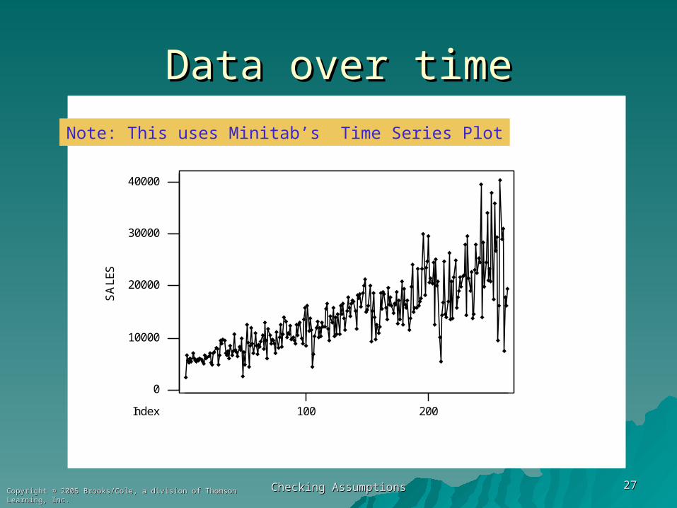
In economic data, however, it is fairly In economic data, however, it is fairly common to see that a variable that common to see that a variable that increases in value often will also increase increases in value often will also increase in scatter.in scatter.


Example 6.3 FOC SalesExample 6.3 FOC Sales

n = 265 months of sales data for a n = 265 months of sales data for a fibre-optic companyfibre-optic company

Y = SalesY = Sales

X= Mon ( 1 thru 265)X= Mon ( 1 thru 265)

Data set FOCSALES6Data set FOCSALES6


Data over timeData over time

40000

30000

20000

10000

0

200100

SA

LES

Index

Note: This uses Minitab’s Time Series Plot


Residual plotResidual plot

3002001000

20000

10000

0

-10000

-20000

Mon

Res

idua

l

Residuals Versus Mon(response is SALES)


ImplicationsImplications

When the errors When the errors eeii do not have a do not have a constant variance, the usual constant variance, the usual statistical properties of the least statistical properties of the least squares estimates may not hold. squares estimates may not hold.

In particular, the hypothesis tests on In particular, the hypothesis tests on the model may provide misleading the model may provide misleading results.results.


6.5.2 A Test for Nonconstant Variance6.5.2 A Test for Nonconstant Variance

Szroeter developed a test that can Szroeter developed a test that can be applied if the observations appear be applied if the observations appear to increase in variance according to to increase in variance according to some sequence (often, over time).some sequence (often, over time).

To perform it, save the residuals, To perform it, save the residuals, square them, then multiply by square them, then multiply by ii (the (the observation number).observation number).

Details are in the text.Details are in the text.


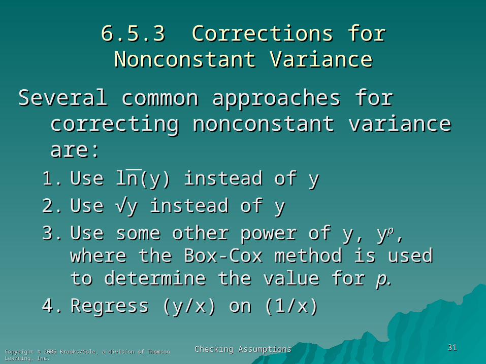
6.5.3 Corrections for Nonconstant Variance6.5.3 Corrections for Nonconstant Variance

Several common approaches for Several common approaches for correcting nonconstant variance are:correcting nonconstant variance are:

1.1. Use ln(y) instead of yUse ln(y) instead of y

2.2. Use √y instead of yUse √y instead of y

3.3. Use some other power of y, yUse some other power of y, ypp, where , where the Box-Cox method is used to the Box-Cox method is used to determine the value for determine the value for p.p.

4.4. Regress (y/x) on (1/x)Regress (y/x) on (1/x)


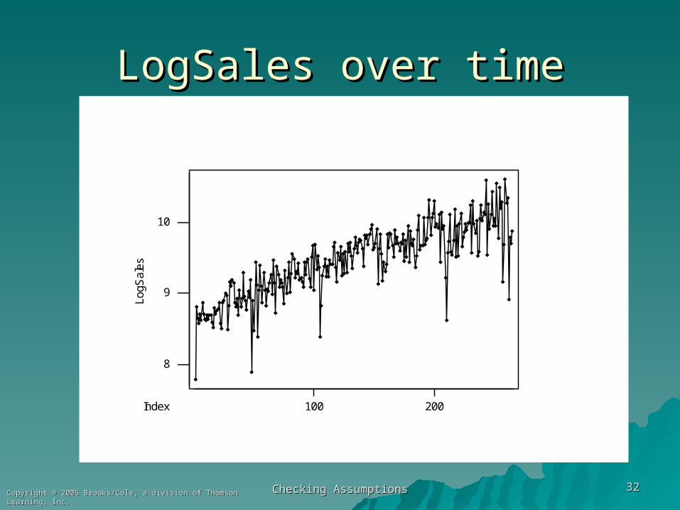
LogSales over timeLogSales over time

10

9

8

200100

LogS

ales

Index


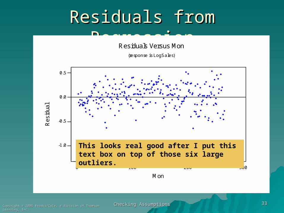
Residuals from RegressionResiduals from Regression

3002001000

0.5

0.0

-0.5

-1.0

Mon

Res

idua

lResiduals Versus Mon

(response is LogSales)

This looks real good after I put this text box on top of those six large outliers.


6.6 Assessing the Assumption That the 6.6 Assessing the Assumption That the Disturbances are Normally DistributedDisturbances are Normally Distributed

There are many tools available to check the There are many tools available to check the assumption that the disturbances are normally assumption that the disturbances are normally distributed.distributed.

If the assumption holds, the standardized If the assumption holds, the standardized residuals should behave like they came from a residuals should behave like they came from a standard normal distribution.standard normal distribution.

– about 68% between -1 and +1about 68% between -1 and +1– about 95% between -2 and +2about 95% between -2 and +2– about 99% between -3 and +3about 99% between -3 and +3


6.6.1 Using Plots to Assess Normality6.6.1 Using Plots to Assess Normality

You can plot the standardized You can plot the standardized residuals versus fitted values and residuals versus fitted values and count how many are beyond -2 and count how many are beyond -2 and +2; about 1 in 20 would be the +2; about 1 in 20 would be the usual case.usual case.

Minitab will do this for you if ask it Minitab will do this for you if ask it to check for unusual observations to check for unusual observations (those flagged by an R have a (those flagged by an R have a standardized residual beyond ±2.standardized residual beyond ±2.


Other toolsOther tools

Use a Normal Probability plot to test Use a Normal Probability plot to test for normality. for normality.

Use a histogram (perhaps with a Use a histogram (perhaps with a superimposed normal curve) to look superimposed normal curve) to look at shape.at shape.

Use a Boxplot for outlier detection. Use a Boxplot for outlier detection. It will show all outliers with an *.It will show all outliers with an *.


Example 6.5 Communication NodesExample 6.5 Communication Nodes

Data in COMNODE6Data in COMNODE6

n = 14 communication networksn = 14 communication networks

Y = CostY = Cost

XX11 = Number of ports = Number of ports

XX22 = Bandwidth = Bandwidth


Regression with unusuals flaggedRegression with unusuals flaggedThe regression equation isCOST = 17086 + 469 NUMPORTS + 81.1 BANDWIDTH

Predictor Coef SE Coef T PConstant 17086 1865 9.16 0.000NUMPORTS 469.03 66.98 7.00 0.000BANDWIDT 81.07 21.65 3.74 0.003

S = 2983 R-Sq = 95.0% R-Sq(adj) = 94.1%


(deleted)

Unusual ObservationsObs NUMPORTS COST Fit SE Fit Residual St Resid 1 68.0 52388 53682 2532 -1294 -0.82 X 10 24.0 23444 29153 1273 -5709 -2.12R

R denotes an observation with a large standardized residualX denotes an observation whose X value gives it large influence.


55000450003500025000

1

0

-1

-2

Fitted Value

Sta

ndar

dize

d R

esid

ual

Residuals Versus the Fitted Values(response is COST)

Residuals versus fits (from regression graphs)Residuals versus fits (from regression graphs)


6.6.2 Tests for normality6.6.2 Tests for normality

There are several formal tests for the There are several formal tests for the hypothesis that the disturbances hypothesis that the disturbances eeii are normal versus nonnormal.are normal versus nonnormal.

These are often accompanied by These are often accompanied by graphsgraphs** which are scaled so that data which are scaled so that data which are normally-distributed which are normally-distributed appear in a straight line.appear in a straight line.

* * Your Minitab output may appear a little different depending on whether you Your Minitab output may appear a little different depending on whether you have the student or professional version, and which release you have.have the student or professional version, and which release you have.


10-1-2

2

1

0

-1

-2

Nor

mal

Sco

re

Standardized Residual

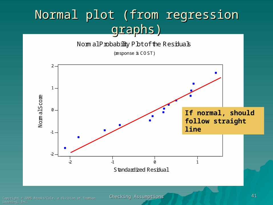
Normal Probability Plot of the Residuals(response is COST)

Normal plot (from regression graphs)Normal plot (from regression graphs)

If normal, should follow straight line


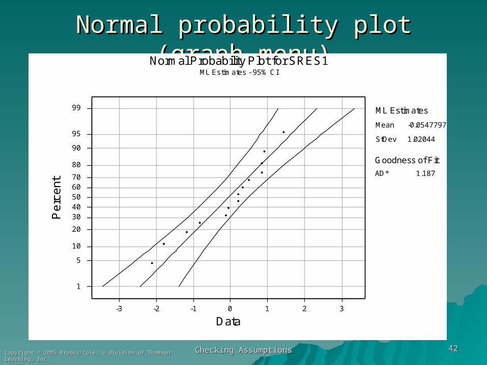
Normal probability plot (graph menu)Normal probability plot (graph menu)

3210-1-2-3

99

95

90

80

7060504030

20

10

5

1

Data

Pe

rce

nt

1.187AD*

Goodness of Fit

Normal Probability Plot for SRES1ML Estimates - 95% CI

Mean

StDev

-0.0547797

1.02044

ML Estimates


Test for Normality (Basic Statistics Menu)Test for Normality (Basic Statistics Menu)

P-Value: 0.216A-Squared: 0.463

Anderson-Darling Normality Test

N: 14StDev: 1.05896Average: -0.0547797

10-1-2

.999

.99

.95

.80

.50

.20

.05

.01

.001

Pro

bab

ility

SRES1

Normal Probability Plot

AcceptsHo: Normality

Part 2Part 2



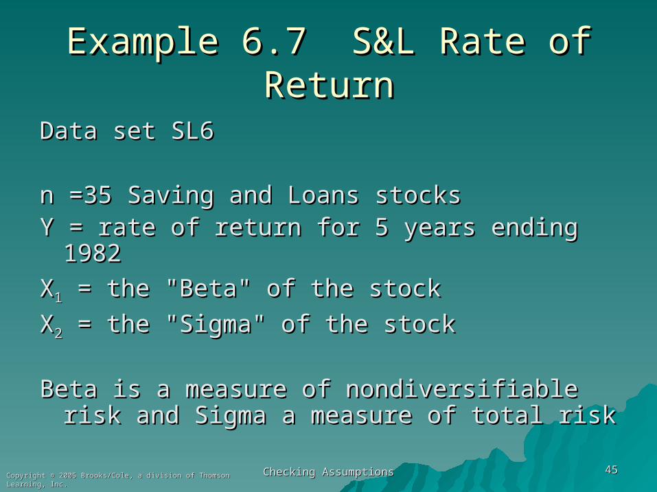
Example 6.7 S&L Rate of ReturnExample 6.7 S&L Rate of Return

Data set SL6Data set SL6

n =35 Saving and Loans stocksn =35 Saving and Loans stocksY = rate of return for 5 years ending 1982Y = rate of return for 5 years ending 1982

XX11 = the "Beta" of the stock = the "Beta" of the stock

XX22 = the "Sigma" of the stock = the "Sigma" of the stock

Beta is a measure of nondiversifiable risk Beta is a measure of nondiversifiable risk and Sigma a measure of total riskand Sigma a measure of total risk


Basic Basic explorationexploration

2.51.50.5

10

5

0

BETA

RE

TU

RN

20100

10

5

0

SIGMA

RE

TU

RNCorrelations: RETURN, BETA, SIGMA

RETURN BETA

BETA 0.180

SIGMA 0.351 0.406


Not much explanatory powerNot much explanatory powerThe regression equation isRETURN = - 1.33 + 0.30 BETA + 0.231 SIGMA

Predictor Coef SE Coef T PConstant -1.330 2.012 -0.66 0.513BETA 0.300 1.198 0.25 0.804SIGMA 0.2307 0.1255 1.84 0.075

S = 2.377 R-Sq = 12.5% R-Sq(adj) = 7.0%

Analysis of Variance (deleted)

Unusual ObservationsObs BETA RETURN Fit SE Fit Residual St Resid 19 2.22 0.300 -0.231 2.078 0.531 0.46 X 29 1.30 13.050 2.130 0.474 10.920 4.69R



One in every crowd?One in every crowd?

43210

5

4

3

2

1

0

-1

Fitted Value

Sta

ndar

dize

d R

esid

ual

Residuals Versus the Fitted Values(response is RETURN)


Normality TestNormality Test

P-Value: 0.000A-Squared: 2.235

Anderson-Darling Normality Test

N: 35StDev: 2.30610Average: 0.0000000

1050

.999

.99

.95

.80

.50

.20

.05

.01

.001

Pro

bab

ility

RESI1

Normal Probability Plot

RejectH0: Normality


6.6.3 Corrections for Nonnormality6.6.3 Corrections for Nonnormality

Normality is not necessary for Normality is not necessary for making inference with large samples.making inference with large samples.

It is required for inference with small It is required for inference with small samples.samples.

The remedies are similar to those The remedies are similar to those used to correct for nonconstant used to correct for nonconstant variance.variance.


6.7 Influential Observations6.7 Influential Observations In minimizing SSE, the least squares procedure In minimizing SSE, the least squares procedure

tries to avoid large residuals.tries to avoid large residuals.

It thus "pays a lot of attention" to y values that It thus "pays a lot of attention" to y values that don't fit the usual pattern in the data. Refer to don't fit the usual pattern in the data. Refer to the example in Figures 6.42(a) and 6.42(b).the example in Figures 6.42(a) and 6.42(b).

That probably also happened in the S&L data That probably also happened in the S&L data where the one very high return masked the where the one very high return masked the relationship between rate of return, beta and relationship between rate of return, beta and sigma for the other 34 stocks.sigma for the other 34 stocks.


6.7.2 Identifying outliers6.7.2 Identifying outliers

Minitab flags any residual bigger Minitab flags any residual bigger than 2 in absolute value as a than 2 in absolute value as a potential outlier.potential outlier.

A boxplot of the residuals uses a A boxplot of the residuals uses a slightly different rule, but should give slightly different rule, but should give similar results.similar results.

There is also a third type of residual There is also a third type of residual that is often used for this purpose.that is often used for this purpose.


Deleted residualsDeleted residuals

If you (temporarily) eliminate the iIf you (temporarily) eliminate the ithth observation from the data set, it observation from the data set, it cannot influence the estimation cannot influence the estimation process.process.

You can then compute a "deleted" You can then compute a "deleted" residual to see if this point fits the residual to see if this point fits the pattern in the other observations.pattern in the other observations.


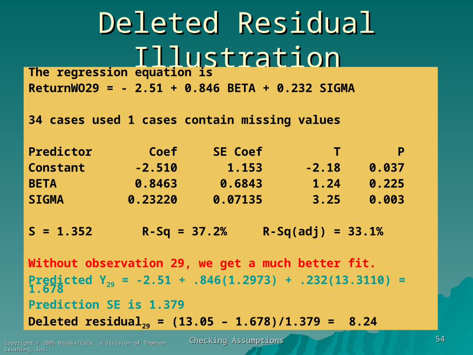
Deleted Residual IllustrationDeleted Residual IllustrationThe regression equation isReturnWO29 = - 2.51 + 0.846 BETA + 0.232 SIGMA

34 cases used 1 cases contain missing values

Predictor Coef SE Coef T PConstant -2.510 1.153 -2.18 0.037BETA 0.8463 0.6843 1.24 0.225SIGMA 0.23220 0.07135 3.25 0.003

S = 1.352 R-Sq = 37.2% R-Sq(adj) = 33.1%

Without observation 29, we get a much better fit.

Predicted Y29 = -2.51 + .846(1.2973) + .232(13.3110) = 1.678Prediction SE is 1.379

Deleted residual29 = (13.05 – 1.678)/1.379 = 8.24


The influence of observation 29The influence of observation 29

When it was temporarily removed, When it was temporarily removed, the Rthe R22 went from 12.5% to 37.2% went from 12.5% to 37.2% and we got a very different equationand we got a very different equation

The deleted residual for this The deleted residual for this observation was a whopping 8.24, observation was a whopping 8.24, which shows it had a lot of weight in which shows it had a lot of weight in determining the original equation.determining the original equation.


6.7.3 Identifying Leverage Points6.7.3 Identifying Leverage Points

Outliers have unusual y values; data Outliers have unusual y values; data points with unusual X values are said points with unusual X values are said to have to have leverageleverage. Minitab flags these . Minitab flags these with an X.with an X.

These points can have a lot of These points can have a lot of influence in determining the Yhat influence in determining the Yhat equation, particularly if they don't fit equation, particularly if they don't fit well. Minitab would flag these with well. Minitab would flag these with both an R and an X.both an R and an X.


LeverageLeverage The leverage of the iThe leverage of the ithth observation is observation is

hhii (it is hard to show where this (it is hard to show where this comes from without matrix algebra).comes from without matrix algebra).

If h > 2(K+1)/n it has high leverage.If h > 2(K+1)/n it has high leverage. For S&P returns, k = 2 and n = 35 so For S&P returns, k = 2 and n = 35 so

the benchmark is 2(3)/35 = .171the benchmark is 2(3)/35 = .171 Observation 19 has a very small Observation 19 has a very small

value for Sigma, this is the reason value for Sigma, this is the reason why it has hwhy it has h1919 = .764 = .764


6.7.4 Combined Measures6.7.4 Combined Measures The effect of an observation on the The effect of an observation on the

regression line is a function of both regression line is a function of both the y and X values.the y and X values.

Several statistics have been Several statistics have been developed that attempt to measure developed that attempt to measure combined influence.combined influence.

The DFIT statistic and Cook's D are The DFIT statistic and Cook's D are two more-popular measures.two more-popular measures.


The DFIT statisticThe DFIT statistic The DFIT statistic is a function of The DFIT statistic is a function of

both the residual and the leverage.both the residual and the leverage.

Minitab can compute and save these Minitab can compute and save these under "Storage".under "Storage".

Sometimes a cutoff is used, but it is Sometimes a cutoff is used, but it is perhaps best just to look for values perhaps best just to look for values that are high.that are high.


DFIT GraphedDFIT Graphed

35302520151050

1.5

1.0

0.5

0.0

Observation Number

DF

IT1

29

19


Cook's DCook's D

Often called Cook's Often called Cook's DistanceDistance

Minitab also will compute these and Minitab also will compute these and store them.store them.

Again, it might be best just to look Again, it might be best just to look for high values rather than use a for high values rather than use a cutoff.cutoff.


Cook's D GraphedCook's D Graphed

35302520151050

0.3

0.2

0.1

0.0

Observation Number

CO

OK

1

19

29


6.7.5 What to do with Unusual Observations6.7.5 What to do with Unusual Observations

Observation 19 (First Lincoln Observation 19 (First Lincoln Financial Bank) has high influence Financial Bank) has high influence because of its very low Sigma.because of its very low Sigma.

Observation 29 (Mercury Saving) had Observation 29 (Mercury Saving) had a very high return of 13.05 but its a very high return of 13.05 but its Beta and Sigma were not unusual.Beta and Sigma were not unusual.

Since both values are out of line with Since both values are out of line with the other S&L banks, they may the other S&L banks, they may represent data recording errors.represent data recording errors.


Eliminate? Adjust?Eliminate? Adjust?

If you can do further research you might If you can do further research you might find out the true story.find out the true story.

You should eliminate an outlier data point You should eliminate an outlier data point only when you are convinced it does not only when you are convinced it does not belong with the others (for example, if belong with the others (for example, if Mercury was speculating wildly).Mercury was speculating wildly).

An alternative is to keep the data point but An alternative is to keep the data point but add an indicator variable to the model that add an indicator variable to the model that signals there is something unusual about signals there is something unusual about this observation.this observation.


6.8 Assessing the Assumption That the 6.8 Assessing the Assumption That the Disturbances are IndependentDisturbances are Independent

If the disturbances are independent, If the disturbances are independent, the residuals should not display any the residuals should not display any patterns.patterns.

One such pattern was the curvature One such pattern was the curvature in the residuals from the linear model in the residuals from the linear model in the telemarketing example.in the telemarketing example.

Another pattern occurs frequently in Another pattern occurs frequently in data collected over time.data collected over time.


6.8.1 Autocorrelation6.8.1 Autocorrelation

In time series data we often find that In time series data we often find that the disturbances tend to stay at the the disturbances tend to stay at the same level over consecutive same level over consecutive observations.observations.

If this feature, called If this feature, called autocorrelationautocorrelation, , is present, all our model inferences is present, all our model inferences may be misleading.may be misleading.


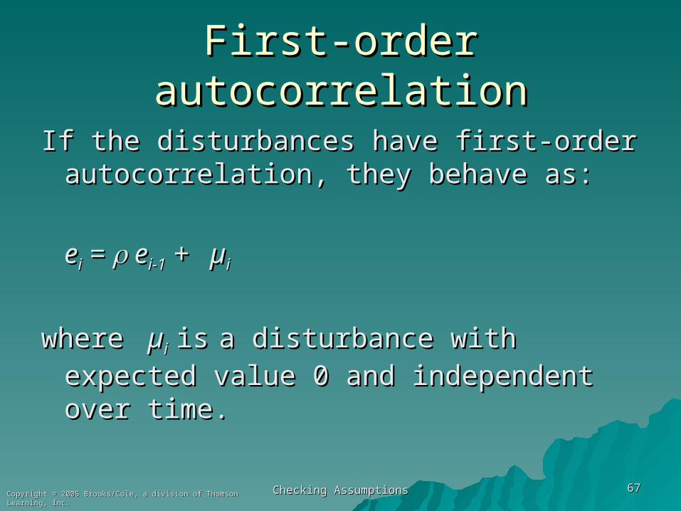
First-order autocorrelationFirst-order autocorrelation

If the disturbances have first-order If the disturbances have first-order autocorrelation, they behave as:autocorrelation, they behave as:

eeii = = e ei-1i-1 + + µµii

where where µ µi i isis a disturbance with a disturbance with expected value 0 and independent expected value 0 and independent over time.over time.


The effect of autocorrelationThe effect of autocorrelation

If you knew that If you knew that ee56 56 was 10 and was 10 and was .7, you would expect was .7, you would expect ee5757 to be 7 to be 7 instead of zero.instead of zero.

This dependence can lead to high This dependence can lead to high standard errors for the bstandard errors for the bjj coefficients coefficients and wider confidence intervals.and wider confidence intervals.


6.8.2 A Test for First-Order Autocorrelation6.8.2 A Test for First-Order Autocorrelation

Durbin and Watson developed a test Durbin and Watson developed a test for positive autocorrelation of the for positive autocorrelation of the form:form:

HH00: : = 0= 0

HHaa: : > > 0 0

Their test statistic Their test statistic d d is scaled so that it is scaled so that it is 2 if no autocorrelation is present is 2 if no autocorrelation is present and near 0 if it is very strong.and near 0 if it is very strong.


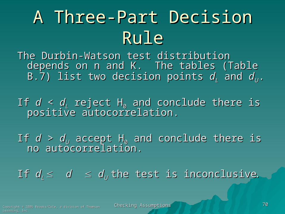
A Three-Part Decision RuleA Three-Part Decision Rule

The Durbin-Watson test distribution depends The Durbin-Watson test distribution depends on n and K. The tables (Table B.7) list two on n and K. The tables (Table B.7) list two decision points decision points ddLL and and ddUU..

If If dd < < ddLL reject H reject H00 and conclude there is and conclude there is positive autocorrelation.positive autocorrelation.

If If dd > > ddUU accept H accept H00 and conclude there is no and conclude there is no autocorrelation.autocorrelation.

If If ddL L dd ddUU the test is inconclusivethe test is inconclusive..


Example 6.10 Sales and AdvertisingExample 6.10 Sales and Advertising

n = 36 years of annual datan = 36 years of annual data

Y = Sales (in million $)Y = Sales (in million $)

X = Advertising expenditures ($1000s)X = Advertising expenditures ($1000s)

Data in Table 6.6Data in Table 6.6


The TestThe Test

n = 36 and K = 1 X-variablen = 36 and K = 1 X-variable

At a 5% level of significance, Table B.7 gives At a 5% level of significance, Table B.7 gives ddLL = 1.41 and= 1.41 and d dUU = 1.52= 1.52

Decision Rule:Decision Rule:

Reject HReject H00 if if dd < 1.41 < 1.41

Accept HAccept H00 if if d d > 1.52> 1.52Inconclusive if 1.41 Inconclusive if 1.41 dd 1.52 1.52


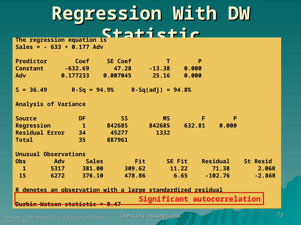
Regression With DW StatisticRegression With DW StatisticThe regression equation isSales = - 633 + 0.177 Adv

Predictor Coef SE Coef T PConstant -632.69 47.28 -13.38 0.000Adv 0.177233 0.007045 25.16 0.000

S = 36.49 R-Sq = 94.9% R-Sq(adj) = 94.8%


Source DF SS MS F PRegression 1 842685 842685 632.81 0.000Residual Error 34 45277 1332Total 35 887961

Unusual ObservationsObs Adv Sales Fit SE Fit Residual St Resid 1 5317 381.00 309.62 11.22 71.38 2.06R 15 6272 376.10 478.86 6.65 -102.76 -2.86R

R denotes an observation with a large standardized residual

Durbin-Watson statistic = 0.47Significant autocorrelation


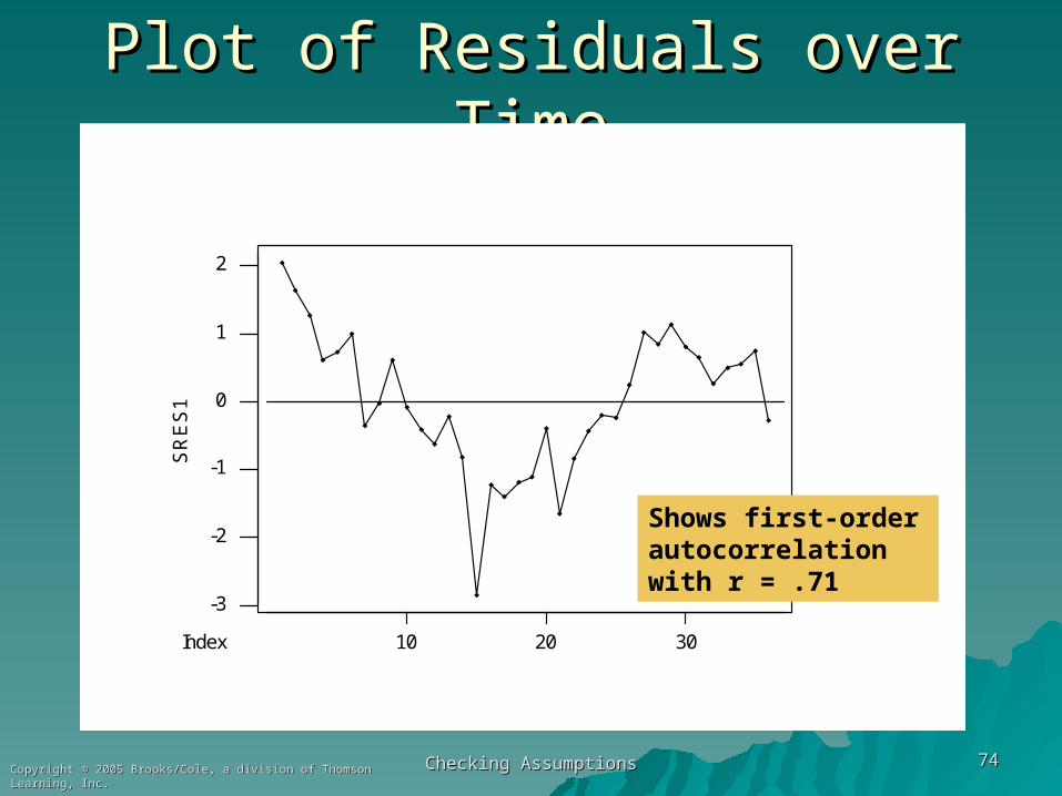
Plot of Residuals over TimePlot of Residuals over Time

2

1

0

-1

-2

-3

302010

SR

ES

1

Index

Shows first-order autocorrelation with r = .71


6.8.3 Correction for First-Order Autocorrelation6.8.3 Correction for First-Order Autocorrelation

One popular approach creates a new y and x One popular approach creates a new y and x variable. variable.

First, obtain an estimate of First, obtain an estimate of . Here we use . Here we use rr = .71 from Minitab's Autocorrelation = .71 from Minitab's Autocorrelation analysis.analysis.

Then compute Then compute yyii* * = y= yii – r y – r yi-1i-1

and and xxii* * = x= xii – r x – r xi-1i-1


First Observation MissingFirst Observation Missing

Because the transformation depends Because the transformation depends on lagged y and x values, the first on lagged y and x values, the first observation requires special observation requires special handling.handling.

The text suggests The text suggests yy11* * = √1 – r= √1 – r2 2 yy11

and a similar computation for and a similar computation for xx11**


Other ApproachesOther Approaches

An alternative is to use an estimation An alternative is to use an estimation technique (such as SAS's Autoreg technique (such as SAS's Autoreg procedure) that automatically adjusts procedure) that automatically adjusts for autocorrelation.for autocorrelation.

A third option is to include a lagged A third option is to include a lagged value of value of yy as an explanatory variable. as an explanatory variable. In this model, the DW test is no In this model, the DW test is no longer appropriate.longer appropriate.


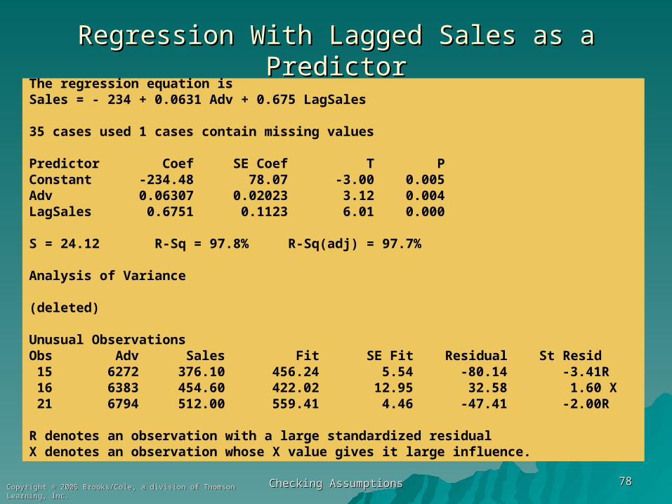
Regression With Lagged Sales as a PredictorRegression With Lagged Sales as a PredictorThe regression equation isSales = - 234 + 0.0631 Adv + 0.675 LagSales

35 cases used 1 cases contain missing values

Predictor Coef SE Coef T PConstant -234.48 78.07 -3.00 0.005Adv 0.06307 0.02023 3.12 0.004LagSales 0.6751 0.1123 6.01 0.000

S = 24.12 R-Sq = 97.8% R-Sq(adj) = 97.7%


(deleted)

Unusual ObservationsObs Adv Sales Fit SE Fit Residual St Resid 15 6272 376.10 456.24 5.54 -80.14 -3.41R 16 6383 454.60 422.02 12.95 32.58 1.60 X 21 6794 512.00 559.41 4.46 -47.41 -2.00R



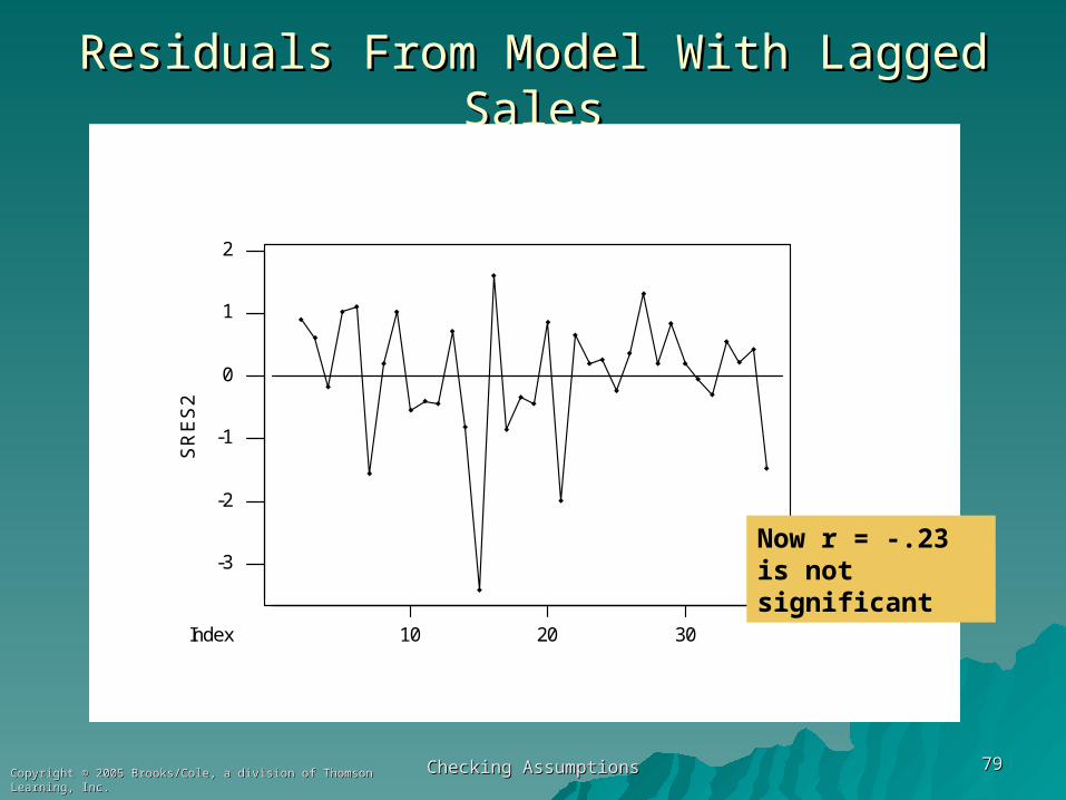
Residuals From Model With Lagged SalesResiduals From Model With Lagged Sales

2

1

0

-1

-2

-3

302010

SR

ES

2

Index

Now r = -.23 is not significant

checking assumptions 1 copyright © 2005 brooks/cole, a division of thomson learning, inc. chapter 6...

Documents

checking assumptions

division of thomson

regression residuals

certain assumptions

standardized residuals

x slide

checking linearity

box plot