1

Notes on Fluidized Bed Design

CHEE 331

January 2013

E.W. Grandmaison

1. Background on fluid-particle systems

2. Background on flow through packed beds

3. Fluid particle systems – fluidization

2

Fluid Particle Systems - Particle Settling Velocity

For theoretical consideration we can examine the behaviour of a single spherical particle

of diameter dp or radius rp and density ρp, freely falling at a velocity U∞ in a fluid of density ρf

and viscosity µf (we could also consider a particle suspended in a gas stream flowing at the

velocity U∞ ). We will assume that the particle concentration is dilute enough that there are no

particle-particle interactions and external forces acting on the particles are negligible (such

forces might include electrostatic effects, etc.).

The forces acting on the particle include:

(1) Gravitational forces:

πρ

63d gp p

(2) Buoyancy forces - equal to the weight of displaced fluid:

πρ

63d gp f

(3) Viscous forces - fluid-particle forces acting at the surface of the particle, commonly called

"friction" drag.

(4) Pressure forces - fluid pressure forces acting over the surface and normal to the particle

surface, commonly called "form" drag.

In general our force balance will have the form:

(1) = (2) + (3) + (4)

Forces (3) and (4) above are more complex and require special attention. We start with the

solution for the velocity and pressure field of a low Reynolds number flow over a sphere. These

solutions are (see for example, Bird, Stewart and Lightfoot, "Transport Phenomena", Wiley,

1960):

( )U U 1 - 32

rr

rrr

p p=

+

∞

12

3

cos θ

( )U - Urr

rr

sinp pθ θ= −

−

∞ 1 3

414

3

3

( )P = P gZ - 32

Ur

rr

coso ff

p

p−

∞ρµ

θ2

x

φ

y

θ

z

U∞

In order to evaluate the "friction" drag, we need to know the shear stress distribution

(spherical coordinate form),

τ µ ∂∂

∂∂θθ

θr f

rrr

Ur r

U= −

+

1

evaluated at the surface of the sphere, i.e.,

( )τµ

θθr r=rp

p

Ur

sin= ∞32

f

and integrate the z-component of this force,

( ) ( )−τ θθr sin

over the surface of the sphere,

( )F = + sin r sin d d r U d Ur r=r00

2

p f p f pp

τ θ

ππ

τ θ θ θ φ πµ πµ∫∫ = =∞ ∞2 4 2

4

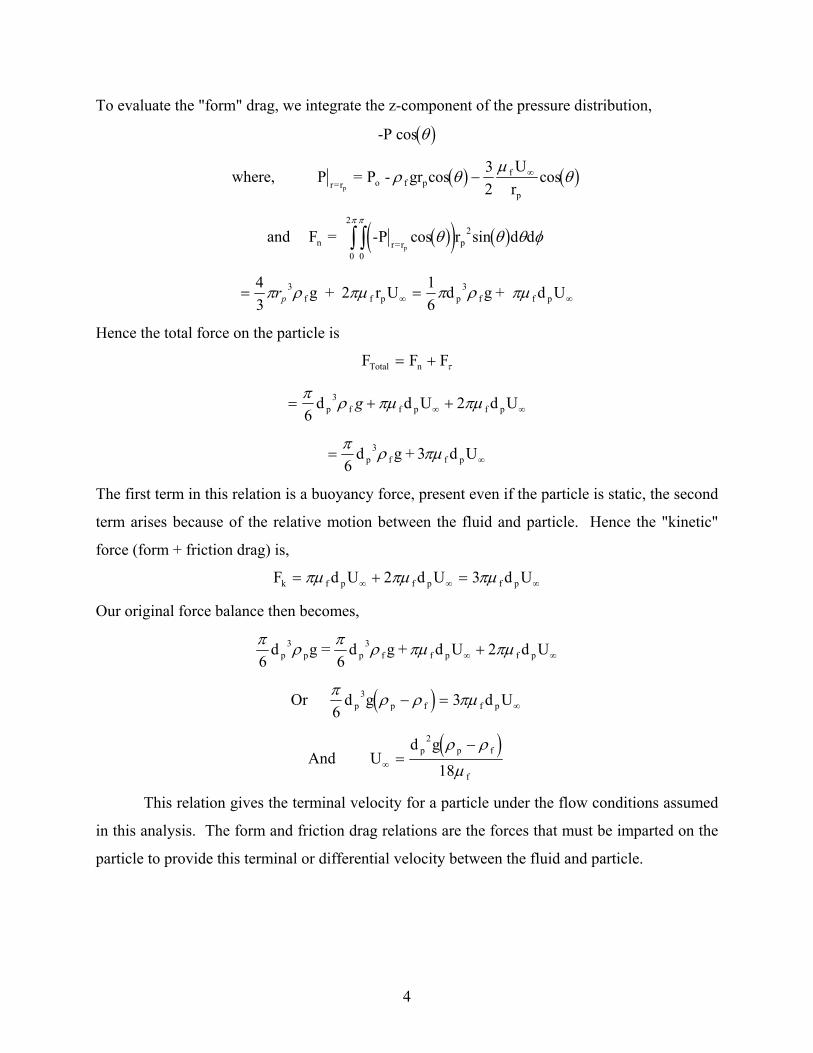
To evaluate the "form" drag, we integrate the z-component of the pressure distribution,

( )-P cos θ

where, ( ) ( )P = P - gr cosU

rcosr=r o f p

f

pp

ρ θµ

θ− ∞32

and ( )( ) ( )F = -P cos r sin d dn r=r00

2

ppθ θ θ φ

ππ

∫∫ 2

= =∞ ∞43

16

3 3π ρ πµ π ρ πµrp f f p p f f pg + 2 r U d g + d U

Hence the total force on the particle is

F F FTotal n= + τ

= + +∞ ∞π ρ πµ πµ6

23d d U d Up f f p f pg

= ∞π ρ πµ6

3d g + 3 d Up f f p

The first term in this relation is a buoyancy force, present even if the particle is static, the second

term arises because of the relative motion between the fluid and particle. Hence the "kinetic"

force (form + friction drag) is,

F d U d U d Uk f p f p f p= + =∞ ∞ ∞πµ πµ πµ2 3

Our original force balance then becomes,

π ρ π ρ πµ πµ6

23 3d g =6

d g + d U d Up p p f f p f p∞ ∞+

Or ( )π ρ ρ πµ6

33d g d Up p f f p− = ∞

And ( )

Ud g

18p p f

f∞ =

−2 ρ ρ

µ

This relation gives the terminal velocity for a particle under the flow conditions assumed

in this analysis. The form and friction drag relations are the forces that must be imparted on the

particle to provide this terminal or differential velocity between the fluid and particle.

5

The assumptions made in the development of the particle settling velocity above included:

1. A low Reynolds number flow, i.e.,

1 U d Nf

fPRe ≤= ∞

µρ

because the relations employed to evaluate the form and friction drag are only applicable

in this regime. The equations of motion for higher Reynolds numbers are too complex

for an analytical solution but we can resort to experimental observations and correlations

for this regime.

2. The fluid acts as a continuum medium. This assumption is important if the particle size

is small (dp < 0.1 µm) thus making the form and friction drag relations inappropriate. To

handle the problem of a lack of continuum between the fluid and particle, the terminal or

settling velocity is multiplied by a correction factor called the Cunningham correction

factor. This problem is encountered in air pollution control systems where small particles

are indeed encountered. We will not meet this problem in CHEE 331.

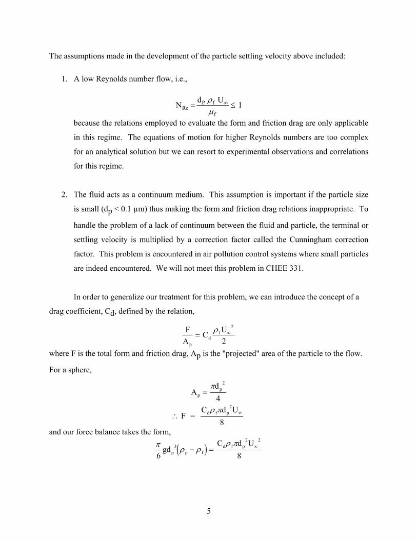
In order to generalize our treatment for this problem, we can introduce the concept of a

drag coefficient, Cd, defined by the relation,

FA

C U

pd

f= ∞ρ 2

2

where F is the total form and friction drag, Ap is the "projected" area of the particle to the flow.

For a sphere,

Ad

pp=

π 2

4

∴ ∞F = C d U

8d f pρ π 2

and our force balance takes the form,

( )π ρ ρρ π

6 83

2 2

gdC d U

p p fd f p− = ∞

6

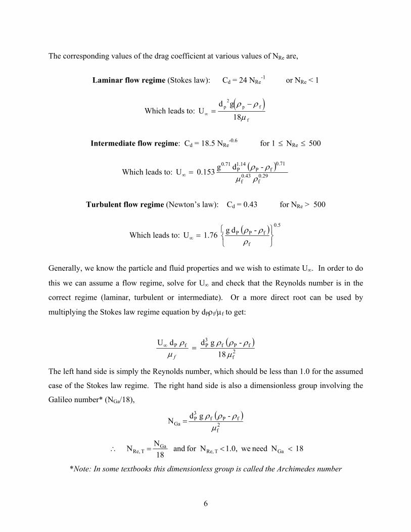
The corresponding values of the drag coefficient at various values of NRe are,

Laminar flow regime (Stokes law): Cd = 24 NRe-1 or NRe < 1

Which leads to: ( )

Ud g

18p p f

f∞ =

−2 ρ ρ

µ

Intermediate flow regime: Cd = 18.5 NRe

-0.6 for 1 ≤ NRe ≤ 500

Which leads to: ( )0.29f

0.43f

0.71fP

1.14P

0.71

- d g 0.153 U

ρµρρ

=∞

Turbulent flow regime (Newton’s law): Cd = 0.43 for NRe > 500

Which leads to: ( ) 5.0

f

fPP - d g 1.76 U

=∞ ρρρ

Generally, we know the particle and fluid properties and we wish to estimate U∞. In order to do

this we can assume a flow regime, solve for U∞ and check that the Reynolds number is in the

correct regime (laminar, turbulent or intermediate). Or a more direct root can be used by

multiplying the Stokes law regime equation by dPρf/µf to get:

( )2f

fPf3PfP

18 - g d d U

µρρρ

µρ

=∞

f

The left hand side is simply the Reynolds number, which should be less than 1.0 for the assumed

case of the Stokes law regime. The right hand side is also a dimensionless group involving the

Galileo number* (NGa/18),

( )2f

fPf3P

Ga - g d N

µρρρ

=

18 N need we1.0, Nfor and 18

N N GaT Re,Ga

T Re, <<=∴

*Note: In some textbooks this dimensionless group is called the Archimedes number

7

Multiplying the Newton’s law regime equation by dPρf/µf we obtain,

( ) 1/2Ga

f

2/1fP

1/2f

1/23/2PfP N 1.76 - g d 1.76 d U

==∞

µρρρ

µρ

f

This means that for the turbulent flow regime (Newton’s law), we need,

80708 Nor 1.76500 N Ga

2

Ga >

>

The intermediate flow regime must then fall between these values for NGa.

We can then write the flow regime criteria as:

Laminar flow or Stokes law (NRe < 1.0): NGa < 18

Intermediate regime (1 < NRe < 500): 18 < NGa < 80708

Turbulent flow or Newton’s law (NRe > 500): NGa > 80708

8

Fluid-Particle Systems - Flow Through Packed Beds

Packed beds of particles are commonly used in the chemical process industries for gas

absorption/adsorption, catalytic reactors and other contacting equipment. One of the main

design objectives for packed beds is to determine the pressure drop requirements. Packed beds

have a relatively low porosity and the pressure drop relationships are based on flow through

tortuous channels. The pressure drop through noncircular ducts is usually based on a

“hydraulic” diameter, dH, defined by

perimeter wallWettedarea sectional cross Flow 4 dH

×=

For a circular tube this concept gives the geometrical diameter, d,

( ) d d

4d 4 d2

H =×

=ππ

and for a concentric tube (inner diameter d1 and outer diameter d2),

[ ]( ) 12

12

21

22

12

21

22

H d - d d dd - d

d d

d - d 4

4 d =

+=

+

×

=π

π

Packed beds also provide complex flow areas and an effective diameter in such a system can be

expressed as

particles of area Surfacebed of volumeVoid dH =

The void volume in a packed bed with porosity ε is

TotalSolidsTotalvoid V V - V V ε==

SolidsSolids V - -1

V ε

=

=

=

εε

ε - 1 V 1 -

- 11 V V SolicsSolidsVoid

For n spherical particles with diameter dP,

=

εεπ - 1

6d n V

3P

Void

and the resulting hydraulic diameter becomes,

9

- 1

6

d d n

- 1

6d n

d P2P

3P

H

=

=εε

πεεπ

A Reynolds number based on the hydraulic diameter is

µρ H

Red U N =

The velocity through the bed material, Ub, and the superficial velocity Us, (the fluid velocity

upstream of the bed with no packed material present) are related by

Us = ε Ub

A Reynolds number through the bed is

µερ

µρ

d U d U N HsHb

Re ==

and substituting for the hydraulic diameter in the bed,

( )εµρ

- 1 d U

61 N Ps

b Re, =

In some derivations, the factor of 4 in the original definition of the hydraulic is not used; this

leads to a coefficient of 2/3 instead of 1/6 in the above relation. Since the Reynolds number will

be used in friction factor empirical relations, the leading coefficient in these expressions is

normally neglected and the Reynolds number is simply expresses as

( )εµρ

- 1 d U N Ps

b Re, =

If we define a friction factor in the general form,

( )2b

H

2b

w

U 21

LP- d U

21 f

ρρ

τ ∆==

where ∆P is the pressure drop through a bed of depth L. Substituting the relations between dH

and dP and Ub and Us, we obtain,

( ) ( )( )ερ

ε

ρ

εε

- 1 U 3 d LP

U 21

LP - 1

6

d

f 2b

P

2b

P

∆−=

∆−

=

10

( )( )ερ

ε - 1 U 3 d LP f and 2

s

3P∆−

=

The factor of 3 is usually neglected in empirical relations for the friction factor-Reynolds number

relationships, i.e.

( )( )

ULP d

1 f 2

s

P3

b ρεε ∆−−

=

Empirical relations for the friction factor through packed beds include:

1. Kozeny-Carman equation (laminar flow):

20 N , N150 f b Re,

b Re,b <=

2. Burke-Plummer equation (turbulent flow): 4

b Re,3

b 10 N 10 , 1.75 f <<=

3. Ergun equation (both regimes):

4b Re,

b Re,b 10 N 1 , 1.75

N150 f <<+=

100 101 102 103 104100

101

102

fb

NRe, b

11

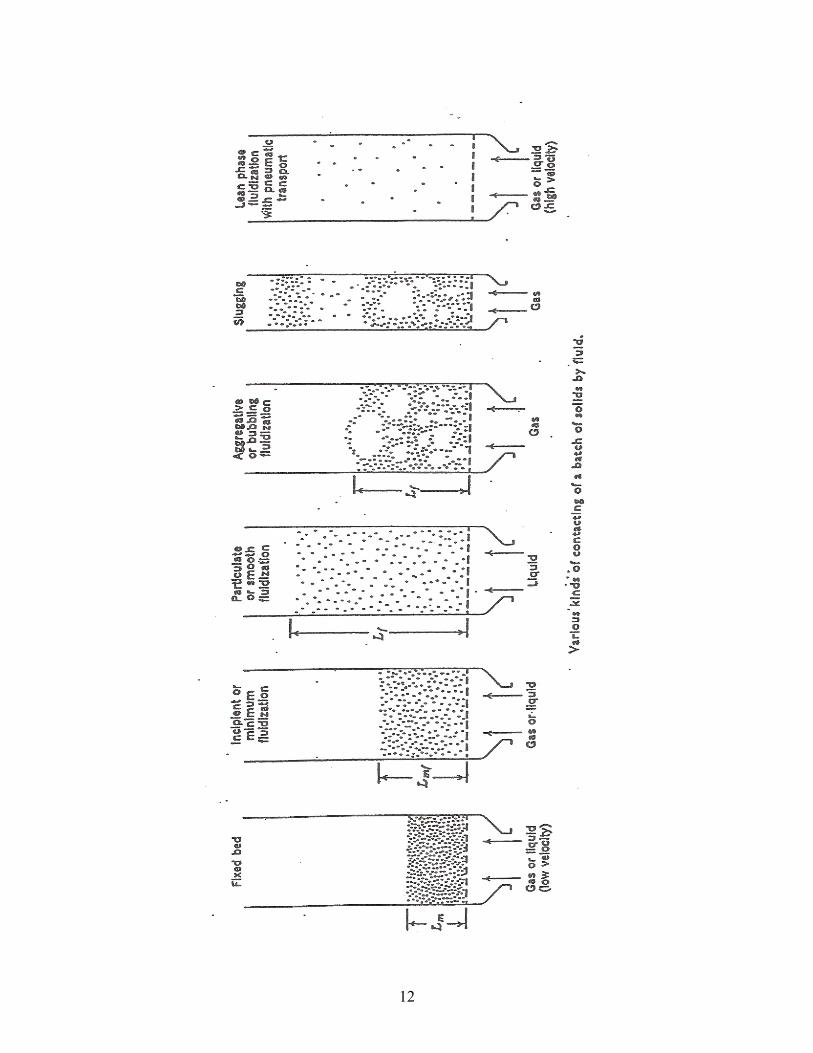
Fluid-Particle Systems - Fluidization

When a fluid passes through a bed of particles at a low flow rate, the fluid initially moves

the void spaces between stationary particles. This flow regime is called a fixed bed. With an

increase in flow rate, the bed passes through several regimes:

Expanded bed: particles move apart, a few vibrate and move about in a restricted manner.

Incipiently fluidized bed: the frictional force between a particle and the fluid counterbalances the

weight of the particle, the vertical component of the compressive force between adjacent

particles disappears, and the pressure drop through any section of the bed is approximately equal

to weight of fluid and particles in that section. This is also called a bed at minimum fluidization.

Smoothly or homogeneously fluidized bed: occurs in liquid-solid systems above minimum

fluidization and results in a smooth, progressive expansion of the bed. Gross flow instabilities

are damped and remain small, and large scale bubbling or heterogeneity is not usually observed.

Aggregative or bubbling fluidized bed: occurs in gas-solid systems above minimum fluidization

and produces large instabilities with bubbling and channelling of the gas. The bed does not

expand as much as the liquid-solid system.

Dense-phase fluidized bed: occurs in both gas and liquid systems at high flow rates as long as

there is a clearly defined upper limit or surface to the bed.

Lean-, disperse-, or dilute-phase fluidized bed: at a sufficiently high fluid flow rate, the terminal

velocity of the solids is exceeded, the upper surface of the bed disappears, entrainment becomes

appreciable, and solids are carried out of the bed with the fluid stream - this leads to pneumatic

transport of the solids.

The general quality of fluidization (slugging, bubbles, etc.) can also be affected by bed

geometry, gas flow rate, type of gas distributor, and vessel internals such as the presence of

screens, baffles, etc.

12

13

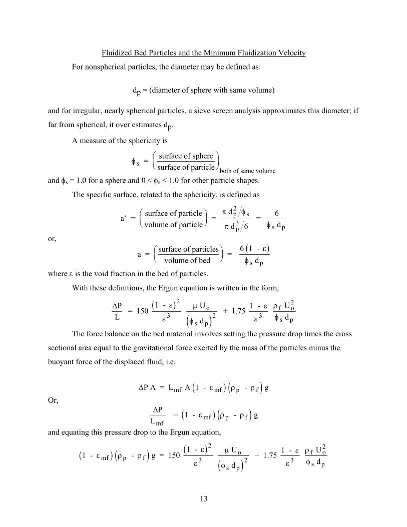
Fluidized Bed Particles and the Minimum Fluidization Velocity

For nonspherical particles, the diameter may be defined as:

dp = (diameter of sphere with same volume)

and for irregular, nearly spherical particles, a sieve screen analysis approximates this diameter; if

far from spherical, it over estimates dp.

A measure of the sphericity is

φ sboth of same volume

= surface of spheresurface of particle

and φs = 1.0 for a sphere and 0 < φs < 1.0 for other particle shapes.

The specific surface, related to the sphericity, is defined as

′

a = surface of particle

volume of particle =

d

d 6 = 6

dp2

s

p3 s p

π φ

π φ

or, ( )

a = surface of particlesvolume of bed

= 6 1 -

ds p

εφ

where ε is the void fraction in the bed of particles.

With these definitions, the Ergun equation is written in the form,

( )

( )∆PL

= 150 1 -

U

d + 1.75 1 -

U d

o

s p3

f o2

s p

ε

ε

µ

φ

ε

ε

ρφ

2

3 2

The force balance on the bed material involves setting the pressure drop times the cross

sectional area equal to the gravitational force exerted by the mass of the particles minus the

buoyant force of the displaced fluid, i.e.

( ) ( )∆P A = L A 1 - - gmf mf p fε ρ ρ

Or,

( ) ( )∆PL

= 1 - - gmf

mf p fε ρ ρ

and equating this pressure drop to the Ergun equation,

( ) ( ) ( )

( )1 - - g = 150

1 -

U

d + 1.75 1 -

U dmf p f

o

s p3

f o2

s pε ρ ρ

ε

ε

µ

φ

ε

ε

ρφ

2

3 2

14

Or multiplying by

( )d

1 - p3

f

mf2

ρ

ε µ

we obtain,

( ) ( )1752

.φ ε

ρ

µ

ε

φ ε

ρ

µ

ρ ρ ρ

µs mf3

p mf f mf

s2

mf3

p mf f p3

f p f2

d U

+ 150 1 -

d U =

d - g

i.e. a quadratic relation for Umf or the Reynolds number. The limit for low Reynolds numbers

gives,

( ) ( )20 < Nfor ,

- 1 g

-

150d

= U Remf

3mffp

2ps

mf

εε

µρρφ

and for high Reynolds numbers, ( )

U = d

1.75

- g , for N > 1000mf

2 s p p f

fmf3

Reφ ρ ρ

ρε

If εmf and/or φs are unknown, Wen and Yu (AIChE Journal, vol. 12, 610, 1966) have shown that

for a wide variety of systems,

1φ ε

ε

φ εs mf3

mf

s2

mf3

14 and 1 -

11≈ ≈

Substitution into the quadratic equation for Umf, we obtain,

( )24.5

d U + 1650

d U =

d - gp mf f p mf f p3

f p f2

ρ

µ

ρ

µ

ρ ρ ρ

µ

2

and the solution to this equation is (taking the positive roots),

( )( )d U

= - 33.7 + 33.7 + 0.0408 d - gp mf f p

3f p f

2

ρ

µ

ρ ρ ρ

µ2

1 2

/

or, ( ) 33.7 - 33.7 N 0.0408 = N 2

Gamf Re, + where NGa is the Galileo number.

15

The low Reynolds number limit is

( )U =

d - g

1650

N = N1650

for N < 20mf

p2

p f

Re, mfGa

Re, mf

ρ ρ

µ

and the high Reynolds number case is,

( )

( )

U = d - g

24.5

N = N24.5

for N > 1000mf2 p p f

f

Re, mf2 Ga

Re, mf

ρ ρ

ρ

and these relations have been found to give predictions of Umf within a standard deviation of ±

34%. If data for εmf and φs are known, they should be used where possible.

16

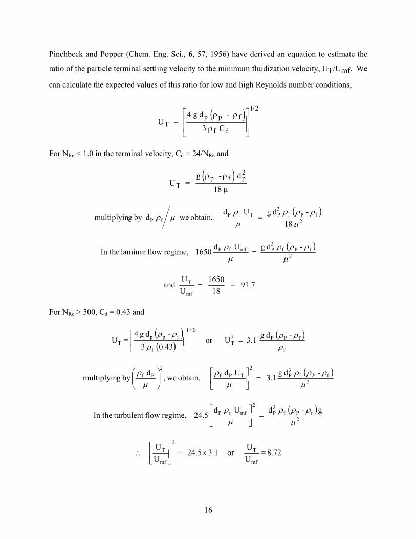
Pinchbeck and Popper (Chem. Eng. Sci., 6, 57, 1956) have derived an equation to estimate the

ratio of the particle terminal settling velocity to the minimum fluidization velocity, UT/Umf. We

can calculate the expected values of this ratio for low and high Reynolds number conditions,

( )U =

4 g d -

3 CTp p f

f d

ρ ρ

ρ

1 2/

For NRe < 1.0 in the terminal velocity, Cd = 24/NRe and

( )U =

g - d

18 Tp f p

2ρ ρ

µ

( )

2fPf

3PTfP

fP 18 - d g U d obtain, we dby gmultiplyin

µρρρ

µρµρ =

( )2

fPf3PmffP - d g U d 1650 regime, flowlaminar In the

µρρρ

µρ

=

91.7 = 18

1650 UU and

mf

T =

For NRe > 500, Cd = 0.43 and

( )( )

( )f

fPP2T

2/1

f

fppT

- d g 3.1 or U 0.43 3

- d g 4 = U

ρρρ

ρρρ

=

( )2

ff3P

2TPf

2Pf - d g 3.1 Ud obtain, we,d by gmultiplyin

µρρρ

µρ

µρ P=

( )2

fPf3P

2mffP g - d U d 24.5 regime, flow turbulentIn the

µρρρ

µρ

=

8.72 = UUor 3.1 24.5

UU

mf

T2

mf

T ×=

∴

17

18

A pressure drop-gas velocity curve for a bed of uniformly sized sand particles is shown

below:

The pressure drop increases approximately linearly with gas velocity up to ∆Pmax at the end of

the fixed bed phase and when Umf is reached, the pressure drop may only increase slightly with

further increases in the gas velocity. This relatively constant ∆P behaviour arises because the

gas-solid phase is well aerated and can deform easily without appreciable resistance. At gas

velocities approaching the terminal velocity of the particles, the pressure drop decreases from the

point of initiation of entrainment. When the gas velocity is decreased, there may be some

hysteresis at low gas velocities (fixed bed regime) due to realignment of the particles from a

random orientation.

Pressure drop behaviour for less than ideal fluidization conditions are shown below for

slugging and channelling:

19

The choice of gas distributor has an effect on the quality of bubbling fluidization:

20

A range of distributor systems are shown in the diagrams below:

21