chemical engineering laboratory (4) - university of jordanengineering.ju.edu.jo/laboratories/lab4...

University of Jordan

Faculty of Engineering and Technology

Department of Chemical Engineering

Chemical Engineering Laboratory

(4)

Manual Sheet

November/2016

Version 5

2




Chemical Engineering Laboratory (4)

Continuous Stirred Tank Reactor

Experiment (1)

Objective

To determine the kinetics and reaction rate constant of the essentially irreversible

reaction between ethyl acetate and sodium hydroxide by the capacity flow method and

to measure the residence time density function of the effluent stream.

Apparatus

Continuous stirred tank reactor-see Fig.(1)- consisting of reaction vessel, two feed

tanks with two pumps, two flow meters and sump tank. Brinkmann pc-600 Probe

Colorimeter, continuous chart recorder and glassware for concentration

measurements.

3

Procedure

Part A

1. Prepare 40 liters of 0.04 M solution of ethyl acetate and 0.04 M sodium

hydroxide , 2 liters of 0.03 M solution of HCl and 0.03 M NaOH

(Chemicals prepared should be standardized).

2. Place the 40 liters solutions into the feed tanks.

3. Switch on the pumps, allow the solutions to be delivered to the reactor at

equal flow rates and set the stirrer to maximum speed.

4. At steady state find the conversion of NaOH.

5. Repeat the experiment at two different flow rates and at the same

temperature.

6. Determine the form of the rate equation between ethyl acetate and sodium

hydroxide.

Part B

1. Fill the reactor with tap water.

2. Calibrate the spectrophotometer-recorder combination by plotting a graph

of transmittance vs pen deflection.

3. At zero time introduce a pulse of colored tracer (phenol red) into the

reactor and record the change of transmittance vs time.

Calculations

1. Determine the reaction rate equation (n, K).

2. Determine E-curve of the effluent stream and determine the reactors flow

model.

References

1. Levenspiel, O., “Chemical Reaction Engineering”, Second Edition, John

Wiley and Sons, 1972.

2. Denbigh, K.G. and Page, F.H., Disc. Faraday Soc., 17 145 (1954).

3. Kendall, H.B., Chem. Eng. Progr. Symp. Ser. 70 (73), 3 (1976).

4. Wen, C.Y. and Chung, S.F., Can. J. Chem. Eng., 43, 101 (1965).

4

Continuous Stirred Tank Reactor's data sheet

Titrants:

Conc. of HCL

Conc. of NaOH

Reactants:

Volume of NaOH sample

Volume of HCl needed for titration

Volume of ethyl acetate sample

Volume of NaOH added

Volume of HCl needed for titration

Item Run 1 Run 2 Run 3

Flow rate of ethyl acetate

Flow rate of sodium

hydroxide

Residence time

Sample 1:

Volume of NaOH

Sample 2:

Volume of NaOH

Sample 3:

Volume of NaOH

Temperature

5





Temperature Measurement

Experiment (2)

Objectives:

1. To be familiar with many different methods of measuring temperature,

highlighting accuracy, calibration and error sensitivity of each in a variety of

working conditions.

2. To introduce the students to the international Temperature Scale, and allows

investigation of the Platinum resistance temperature measurement method that

forms a fundamental part of the standard.

Equipment:

The unit consists of a small bench mounted Console contains a number of different

instruments and connection points for sensors. A temperature controlled heater plate

is also available as well as a computerized data acquisition system with computer

monitor and printer. The sensors available are: Platinum Resistance, Thermistor, &

three types of thermocouple. A vacuum flask and stainless steel beaker are also

available

Theory:

Temperature can be defined technically as an indication of intensity of molecular

activity. The temperature of a body is a measure of the thermal potential of that body

and determines whether heat is supplied to or rejected from the body when in contact

with a body at different temperature.

Different scales are used in thermometry such as Centigrade scale which is based on

the point at which ice melt and pure water boils at standard atmospheric pressure. The

Celsius scale indicated that the ice point be substituted by the triple point which in the

state of pure water existing as a mixture of ice, liquid and vapor in equilibrium, and

equals 0.01°celsius. Another scale is the Kelvin scale, and another one is the

international temperature scale.

6

Procedure:

Several experiments can be performed in the temperature measurement unit:-

Exp. No. 1

The use of liquid in glass thermometer, Vapor pressure & bi-metallic expansion

devices for measurement of fixed scale point.

1. Partially fill the vacuum flask with ice and water and place one of the glass

tube thermometers in the mixture.

2. Fill 2/3 of the stainless steel beaker with pure water and place rubber disc on

top, place the beaker on heater plate and turn on the main switch. Set the

heater plate to a temperature of about 200°C.

3. Once the water has reached boiling point, turn the temperature setting down to

about 120°C.

4. Record the temperature of the water in the beaker and in the vacuum flask.

5. Repeat using vapor pressure thermometer & the bi-metallic expansion

thermometer instead of liquid in glass thermometer.

Exp.No.2

Response of different temperature measuring devices as temperature changes

with time.

1. Fill 2/3 of the stainless steel beaker with pure water and place rubber disc on

top, place the beaker on heater plate and don’t turn on the main in this stage.

2. Place the Glass thermometer, Platinum resistance, Thermistor and the

Thermocouple in the unheated water in the beaker and switch on the heater

plate and set the heater plates to temperature 200°C.

3. Start recording the temperature using the computerized unit.

4. Record the temperature of the thermometer each 30 sec.

5. Once the water has reached boiling point, turn the heater off and stop

recording.

7

Exp.No.3

a- The Peltier thermo-electric effect.

1. Partially fill the vacuum flask with ice and water, and fill 2/3 of the stainless

steel beaker with pure cold water and place rubber disc on top, place the

beaker on heater plate and don’t turn on the main in this stage.

2. Put water in a beaker and measure the ambient temperature by using the glass

thermometer.

3. Select one of the shrouded type K thermocouple and do the instructed

connection.

4. Now place the thermometer with the thermocouple in the unheated water in

the beaker and switch on the heater plate and set the heater plate to

temperature of about 200°C.

5. Start recording the temperature and millivolt signal by using the computerized

unit.

6. Record the temperature of the thermometer each 30 sec.

7. Once the water has reached 40°C, stop recording and turn the temperature

setting down to about 120°C.

b- Seebeck effect.

1. Select two of the shrouded type K thermocouples and connect them as

instructed.

2. Place BOTH thermocouples in the vacuum flask and record the millivolt.

3. Place one thermocouple in the stainless steel beaker on the hot plate together

with a glass thermometer, and record the millivolt.

4. Place the thermocouple that has been immersed in the vacuum flask into the

hot water with the other thermocouple, note the millivolt reading.

5. Now reverse the positions of the thermocouples (Hot beaker thermocouple to

vacuum flask), and record the millivolt.

8

Exp. No. 4

Voltage calibration of different thermometer types using water-ice reference.

1. Select two of the shrouded type K thermocouples.


steel beaker with pure water and place rubber disc on top, place the beaker on

heater plate and don’t turn on the main in this stage.

3. Connect the two thermocouples as instructed, and put one of the thermocouple

in vacuum flask and the other in the beaker with a glass thermometer.

4. Plug in the Platinum resistance plug and the Thermistor plug to the unit and

place the probes in the water in the beaker.

5. Switch on the heater plate and set the temperature to 200°C.

6. Start recording the temperature and the millivolt signal by using the

computerized unit at regular intervals until the water boils.

Exp. No. 5

The law of intermediate metals and intermediate temperature associated with

thermocouple.

1. Select two of the shrouded type K thermocouples.


steel beaker with pure water and place rubber disc on top, place the beaker on

heater plate and don’t turn on the main in this stage.

3. Connect the two thermocouples as instructed by using the two green

thermocouple extension leads supplied, and put one of the thermocouple in

vacuum flask and the other in the beaker.

4. Switch on the heater plate and set the temperature to 200°C. Once the water

has reached boiling point, turn the temperature setting down to about 120°C.

5. Record the millivolt reading.

6. Immerse either junction A, B, or C in the ice-water mixture or the boiling

water and record the millivolt.

7. Break the junction B and rejoin this using a RED or BLACK copper

connecting lead, and record the millivolt.

8. Immerse the two new junctions either in the ice-water or boiling water, and

record the millivolt.

9. Remove the RED or BLACK copper lead and record the millivolt.

9

10. Take the thermocouple from the ice-water and hold it in your hand until the

millivolt meter display is constant and then record the millivolt.

11. Replace the thermocouple in the ice-water and allow the millivolt meter to

return to its original reading.

12. Now remove the other thermocouple from the boiling water ALLOW TO

COOL SLIGHTLY and then hold in your hand as before until the millivolt

meter display is constant and record the millivot reading.

Exp. No. 6

Connection of thermocouple in parallel for averaging of measured temperature

and series for signal amplification

1. Partially fill the vacuum flask with cold water, and fill 2/3 of the stainless steel

beaker with pure water and place rubber disc on top, place the beaker on

heater plate and turn on the main switch. Set the temperature to about 200°C.

2. Once the water has reached 70°C, turn the temperature setting down to about

120°C.

3. For parallel; select two of the type K thermocouples, connect the two type K

thermocouple to any two of the thermocouple sensor sockets.

4. Place one thermocouple in the vacuum flask and the other in a beaker, full of

hot water of about 70°C.

5. Depress the switches INDIVDUALLY and record the temperature. Then

depress both switches together and record the temperature.

6. For Series; select four type K thermocouples (two shrouded and two exposed

tip) and connect them as instructed.

7. The BLACK thermocouples plugs are shown as B, the RED thermocouples

plugs are shown as R, the thermocouples junctions are shown as K. The pair of

thermocouples shown as H are in the stainless steel beaker and the pair of

thermocouples shown as C are shown in the vacuum flask.

8. Once the water in the stainless steel beaker starts boiling, observe and record

the millvolt meter display.

10

Calculation:

Each number indicates to experiment number:

1. Record the temperature of the water by using Glass thermometer, Vapor

pressure, Bi-metallic expansion device, Platinum resistance, Thermistor &

Thermocouple, and explain why the temperature doesn’t reach 0°C and 100

°C.

2. Plot the temperature readings of the devices used versus time and note the

response of each measuring device.

3. Record the reading of millivolt as indicated and explain the negative reading

you get in both Peltier thermo-electric effect & Seebeck effect.

4. Refer to the tables in the lab sheet for a type of thermocouple that you used in

this experiment showing the millivolt signal and corresponding temperature

when the reference junction is held at 0°C and at each temperature reading,

compare between the recorded millivot reading and the millivolt from the

table that corresponds to that temperature.

5. Record the reading of millivolt as indicated and explain your results.

6. Record the reading of millivolt as indicated and explain your results.

11

Temperature Measurement

Part 1

Thermometer Temperature (C ) Glass thermometer

Vapor pressure Bi-metallic

Platinum resistance Thermistor

Thermocouple

Part 2

Time Temperature (C )

Glass thermometer

12

Part 3

a- Peltier thermo-electric:

Ambient temperature:

Time Temperature (C )

Glass thermometer

b- Seebeck effect:

Voltage

Both thermocouples in cold water

Thermocouple (1) in cold and (2) in hot

Thermocouple (2) in cold and (1) in hot

13

Part 5

Intermediate metal:

Voltage for the junction without intermediate metal:

Voltage

Junction A in hot water Junction B in hot water Junction C in hot water

Junction A in ice Junction B in ice Junction C in ice

Voltage for the junction with intermediate metal:

Voltage

Junction B in hot water Junction B’ in ice

Intermediate Temperature:

Voltage

E hot – E ice E hot-E hand E hand- E ice

Part 6

Parallel connection: Series connection:

Temp by depress switch # 1

Voltage = Temp by depress switch # 2 Temp by depress switch # 3

Temp by depress switch #

1+2

Temp by depress switch #

1+2+3

14





TEMPERATURE MEASUREMENT(PART 1)

Experiment (2)

1-THE PELTIER THERMOELECTRIC EFFECT:

Objective: To demonstrate the temperature dependent of electrical potential produced

by dissimilar metals in contact.

Equipment: See the attached sheet.

Theory:

The Peltier thermoelectrical effect (1834) can be stated as follows: current flowing

across a junction of dissimilar metals causes heat to be absorbed or liberated. The

direction of heat flow can be reversed by reversing the current flow. The rate of heat

is proportional to temperature versus the voltage reading.

Requirement: plot the measured temperature versus the voltage reading.

2-THE SEEBECK THERMO-ELECTRICAL EFFECT:

Objective: To demonstrate the resultant electromotive force produced in a

thermocouple circuit.


Theory:

The Seebeck effect or Seebeck principle discovered by T.J Seebeck (1821) states that

an electric current flows in a circuit of two dissimilar metals if the two junctions are at

different temperatures.

15

In figure 1: The temperature of the hot junction is the temperature being measured

and Tc is the cold junction temperature or the reference temperature. The most

common thermocouples are: platinum-rhodium/platinum, chromel/alumel, and

copper/constantan. The circuit in figure 1 can be used for temperature measurement

as shown as in figure 2. In chemical industries, sometimes it is not possible to

maintain the cold junction at 0 C. Normally, the cold junction is at ambient

temperature, with correction is made automatically by temperature-sensitive resister.

Fig.(1): Electro-thermal circuit of two dissimilar metals.

Fig.(2): Thermocouple circuit.

References:

1. Shahian, B. and Hassul, M., Control System Design. Prentice Hall, 1993.

2. Considine, D., M., Process Instruments and Control Handbook. McGraw-

Hill, 1974.

M

M

M

Reference junction

Measuring junction

16






Experiment (2)

1-THE LAWS OF INTERMEDIATE METALS AND

TEMPRETURES:

Objective: To demonstrate the effect of introducing different types of metals in a

thermocouple circuit, and the principle of intermediate temperature


Theory:

Several thermoelectric laws have been established experimentally by measuring the

current resistance, and emf in thermoelectric circuits. These laws are experimentally

accepted despite the lack of theoretical development. In fact, we need not to

understand the complexities of electron-phonon (the quantum particles of thermal

conduction waves) to understand the working principles of thermocouples. We need

only to pay attention to the understanding the laws of thermoelectricity.

1-Law of homogeneous materials:

A thermoelectric current cannot be sustained in a circuit of a single homogeneous

material by the application of heat alone. A fact could be drawn from this law that

two different types of metals are required to construct any thermocouple circuit.

Experiments have shown that a measurable thermoelectric current flows in a circuit if

a nonsymmetrical temperature gradient is set up in a homogeneous wire. This for no

doubt is attributed to non-homogeneous metals.

2- Law of intermediate metals:

The algebraic sum of the thermoelectromotive forces in a circuit composed of any

dissimilar metals is zero provided that all of the circuit is at a uniform temperature.

17

A consequence of this law is that a third homogeneous wire can be added in a

thermocouple circuit as long as its extremities are kept at the same temperature. So a

device for measuring the thermoelectromotive force can be introduced into a circuit at

any point without effecting the net emf if all the connections at the same temperature.

In Figure 1:if T1=T2, then from the Seebeck principle the net emf is zero.

3- Law of successive or intermediate temperatures:

If two dissimilar homogeneous materials produce a net emf of , 0it tE when the two

junctions are at T, TI, the emf generated when the junctions are at T and T0 is given by:

0 0, , ,I IT T T T T TE E E (1)

Figure (1): Thermocouple circuit with intermediate metal type C.

Equation (1) is evident from Figure 2 and the Seebeck principle:

Figure (2): Emfs are additive for materials.

, IT T IE T T

TT

A

T c

Metal C

T T

18

, 0 0iT T IE T T

0, 0T TE T T

0 0, , 0 0 ,I IT T T T I I T TE E T T T T T T E

Note that equation 1 follows from the last result, where IT satisfies: 0 IT T T .

Questions:

1. A thermocouple of type J (iron-constantan) has the following input-output

data from standard tables:

T ( C ): 0 30 300

emf (mV): 0 1.5 15

2. Discuss the validity of the law of intermediate temperatures on the basis of

Seebeck principle over a wide temperature range (0 t0 500 C).

References:

1. Considine, D. M., Process instruments and control handbook. McGraw-Hill,

1974.

2. Benedict, P. E., Fundamentals of temperature, pressure and flow

measurements. John Wiley, 1984.

3. Bolton, W., Mechatronics: electronic control systems in mechanical

engineering. Longman, 1997.

19






Experiment (2)

Objectives: To understand the static and dynamic characteristics of measuring

devices and in particular temperature measuring devices


Temperature Sensors: One of the most important variables in chemical industries is the temperature. It is not

only used as a direct control variable, but also as a means to infer about other

controlled variables (inferential control). Table 1 below shows the most popular

sensors used for temperature measurement.

The term sensor is used to identify an element that produces a signal when subjected

an input physical change. Often the term transducer is used interchangeably with the

term sensor.

Table 1 Important Sensors (Transducers) for Temperature

Measurement.

I. Expansion thermometers

A. Liquid-in-glass thermometers

B. Solid-expansion thermometers (bimetallic strip)

C. Filled-system thermometers (pressure

thermometers)

1. Gas-filled

2. Liquid-filled

3. Vapor-filled

II. Resistance-sensitive devices

A. Resistance thermometers

B. Thermistors

III. Thermocouples

20

1. Expansion thermometers:

Liquid-in-glass thermometers: indicate temperature change caused by

the difference between the temperature coefficient of expansion for glass and

the liquid employed. Mercury and alcohol are the most widely used liquids.

2. Solid Expansion thermometers (Bimetallic strip):

Bimetallic strip thermometer: The working principle depends on

different expansion coefficients of metals as a function of temperature. Fig(1)

shows a typical bimetallic strip thermometer. The temperature-sensitive

element is a composite of two different metals fastened together into a strip. A

common combination is invar (64% Fe, 36% Ni), which has a low coefficient,

and another nickel-iron alloy that has a high coefficient.

Fig.(1): Details of bimetallic strip thermometer [1].

3. Filled-system thermometers (pressure thermometers):

A typical filled-system thermometer. is shown in Fig.(2) The fluid expands or

contracts due to temperature variations which is sensed by the Bourdon

spring and transmitted to an indicator or transmitter. These elements are

popular in the chemical process industries.due to their design simplicity and

relatively low cost.

Resistance thermometers Devices(RTD): Fig.(3) shows RTD which

based on the principle that the electrical resistance of pure metals increases

with an increase in temperature. This provides an accurate way to measure

temperature because measurements of electrical resistance can be made with

high precision.

21

Fig.(2): Filled system thermometer [1,4].

The resisitance of most metals increases linearly with temperature:

0(1 )tR R Ta= + (1)

The most commonly used metals are platinum, nickel, tungsten, and copper. A

Wheatstone bridge is generally used for the resistance reading and, consequently, for

the temperature reading.

Fig.(3): Resistance thermometer device (RTD): a- Assembly. b- Components [1,4].

22

1. Thermistors:

Modern thermistors are usually mixtures of oxides such as the oxides of

nickel, manganese, iron, copper, cobalt and titanium, other metals and doped

ceramics. The material is formed into various forms such as beads discs and

rodes as shown in Fig.(4). Thermistors can have either a negative temperature

coefficient (NTC), where the resistance decreases with temperature, or a

positive temperature coefficient(PTC) depending on the type of materials used.

They were originally named from a shortened form of the term thermally

sensitive resistor. The resistance-temperature relationship can be described by:

/ TR Keb= (2)

Where K and b are constants.

Fig.(4): Thermistor construction [2,4].

Fig.(5): Thermocouple circuit

2. Thermocouples:

The thermocouple is the best-known industrial temperature sensor. It works on

a principle discovered by Seebeck in 1821. The Seebeck effect, or Seebeck

principle, states that an electric current flows in a circuit of two dissimilar metals

if the two junctions are at different temperatures. Fig.(4) shows a simple

23

circuit in which M1 and M2 are the two metals, TH is the temperature being

measured, and TC, is reference temperature. The voltage produced by this

thermoelectric effect depends on the temperature difference between the two

junctions and on the metals used.

Static Characteristics:

The output values given when steady state condition is attained, after a certain

input is received, are known as static characteristics of the sensor. The most

important static characteristics are:

1. Range: The limits between which the input can vary.

2. Error: The difference between the true (standard) value and the result of

measurement.

3. Accuracy: The extent to which the value indicated by the measuring device is

wrong. It is the sum of all the possible expected errors including the

calibration accuracy.

4. Precision: It describes an instrument’s degree of freedom from random errors.

If a large number of readings are taken of the same quantity by a high

precision instrument, then the spread of readings will be very small.

5. Repeatability: It describes the closeness of output readings form the

measuring device when the same input is applied repetitively over a short

period of time, with the same measurement conditions, same instrument and

observer, same location and same conditions of use maintained throughout.

6. Reproducibility: describes the closeness of output readings for the same input

when there are changes in the method of measurement, observer, measuring

instrument, location, conditions of use and time of measurement. Fig.(6)

compares the accuracy, repeatability and reproducibility.

7. Sensitivity: Sensitivity is the ratio of the change in response of an instrument

to the change in the stimulus (how much output you get per unit input).

8. Hysteresis: The difference between the measuring device readings during a

continuously increasing and decreasing change of the input. Fig.(7) shows a

typical hysteresis curve.

24

Fig.(6): Comparison of accuracy and precision.

Fig.(7): Measuring device static characteristics with hysteresis.

Dynamic Characteristics:

The dynamic characteristics of a measuring instrument describe its behaviour between

the time the input value changes and the time the instrument output attains a steady

value in response.

Target

25

In any linear, time-invariant measuring system, the following general relation can be

written between input and output for time t > 0:

1

0 011 1...

n n

n n nn

d y d y dya a a a y b u

dt dtdt

-

--+ + + = (3)

Where y and u are the output and input respectively, 0 1, , ... na a a and

0b are constant

model parameters.

1. Zero-order dynamics: An instrument is said to show zero-order dynamics, if

it responds instantaneously to the applied input. Mathematically, this means

that:1 1

... 0n na a a-

= = = . Consequently, the instrument sensitivity

(gain) is given by:

0

0

e

byK

u a

D= =

D (4)

Fig.(8) shows the response of such instrument.

Fig.(8): Zero-order instrument dynamic response.

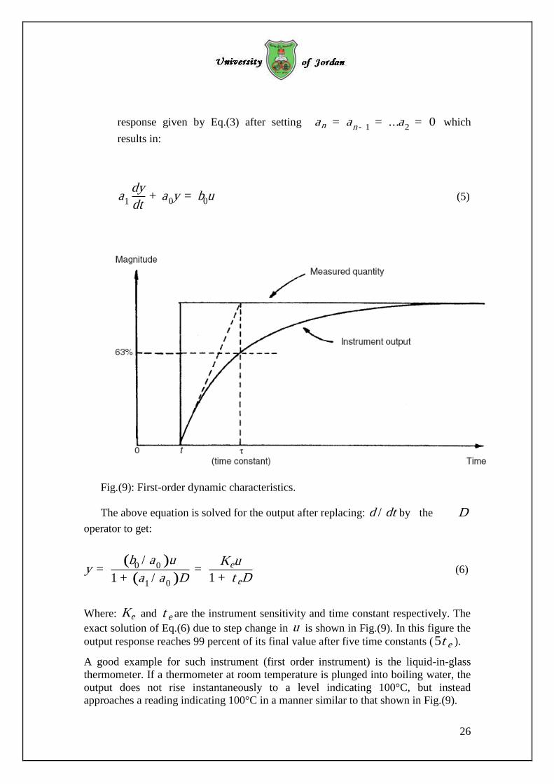
2. First-order dynamics: An instrument is said to show first-order dynamics, if

it reaches 63 percent of the final steady state value after a time equals one

instrument time constant. First-order dynamic instruments follow a dynamic

26

response given by Eq.(3) after setting 1 2

... 0n na a a-

= = = which

results in:

0 01

dya a y b u

dt+ = (5)

Fig.(9): First-order dynamic characteristics.

The above equation is solved for the output after replacing: /d dt by the D

operator to get:

( )

( )0 0

01

/

11 /e

e

b a u K uy

Da a D t= =

++ (6)

Where: eK and et are the instrument sensitivity and time constant respectively. The

exact solution of Eq.(6) due to step change in u is shown in Fig.(9). In this figure the

output response reaches 99 percent of its final value after five time constants (5 et ).

A good example for such instrument (first order instrument) is the liquid-in-glass

thermometer. If a thermometer at room temperature is plunged into boiling water, the

output does not rise instantaneously to a level indicating 100°C, but instead

approaches a reading indicating 100°C in a manner similar to that shown in Fig.(9).

27

Requirements:

1. Study experimentally the static and dynamic characteristics of the available

temperature measuring instruments in the Lab.

2. Investigate the dynamic linearity of the selected temperature sensor using the

mirror image method.

References:

1. Smith, C. A. & Corripio, A. B. (1997). Principles and practice of automatic

process control, John Wiley & Sons, New York.

2. Morris, A. S. (2001). Measurement and Instrumentation Principles.

Butterworth- Heinemann, Oxford.

3. Shahian, B. and Hassul, M., Control System Design. Prentice Hall, 1993.

4. Considine, D., M., Process Instruments and Control Handbook. McGraw-

Hill, 1974.

28





Batch Reactor

Experiment (3)

Objectives

1. To find the reaction rate constant for Saponification reaction in a batch

reactor.

2. To study the effect of varying process conditions on the reaction rate constant.

Apparatus

The batch reactor vessel is a double skinned glass vessel with one liter and a half of

internal working volume, the reactor is mounting on a computer controlled chemical

reactors service unit which also provides the ancillary services for the reactor. The

reactor is equipped with an agitator driven by an electric motor and controlled using

the Armfield software. The speed can be varied using the up/down arrows or by

typing in a value between 0-100%-see figures (1) & (2). A clear, acrylic, self-

contained hot water circulator is positioned on the unit at the front right hand side-see

figure (3)-this vessel incorporates an element for heating water, a thermostat and level

detector are incorporated in the vessel to prevent the heater from operating if the

water is too hot or the level in the vessel is too low. A thermocouple sensor T2 is

supplied with this unit to measure the fluid temperature in the vessel. Flexible tubes

are used to connect the circulator to the reactor. Water, heated by an electrical heating

element in the circulator, is circulated by a gear pump located at the back of the plinth

behind the vessel. Temperature control is achieved by circulation of heated water

through the jacket of the batch reactor. T1 is designed to be used individually with

reactors in conjunction with the PID controller in the software and T2 is to be used

with hot water circulator vessel. A conductivity probe is supplied to be used with the

reactor, the conductivity is displayed on the software in units of millisimens/cm.

During the chemical reaction, the conductivity of the reacting solution changes as

more of the reactants are converted. This data can be logged and used to determine the

degree of conversion and the rate of reaction.

30

Theory

The Armfield batch reactor is designed to demonstrate the mechanism of a chemical

reaction in a reactor, as well as the effects of varying process conditions such as

reaction temperature and reagents concentrations. In this experiment, the

Saponification of Ethyl acetate by Sodium hydroxide is the reaction chosen to study

these conditions.

NaOH+CH3COOC2H5 → CH3COONa+C2H5OH

For this second order elementary reaction the rate equation is:

-rA=k.CA.CB (1)

Where,

rA = rate of reaction (mol.L-1

.S-1

)

K = reaction rate constant (S-1

)

CA = concentration of NaOH (mol.L-1

)

CB = concentration of Ethyl acetate (mol.L-1

)

If the initial concentrations of reactants are equal, then:

-dCA/dt = k.CA2 (2)

Integration of this rate law for a single reactant gives;

1/CA=k.t+1/CAo (3)

t = time (s)

CAo = initial concentration of NaOH (mol.L-1

)

Hence, a plot of 1/CA against t gives a straight line of gradient k and an intercept of

1/CAo

If the initial concentrations of reactants are not equals, then the rate equation above

should be combined with the following equations:

𝜃 = CBo/CAo (4)

XA = (CAo – CA)/ CAo (5)

CB = CBo- CAoXA (6)

Where,

CBo = initial concentration of Ethyl acetate (mol.L-1

)

XA = conversion of NaOH

31

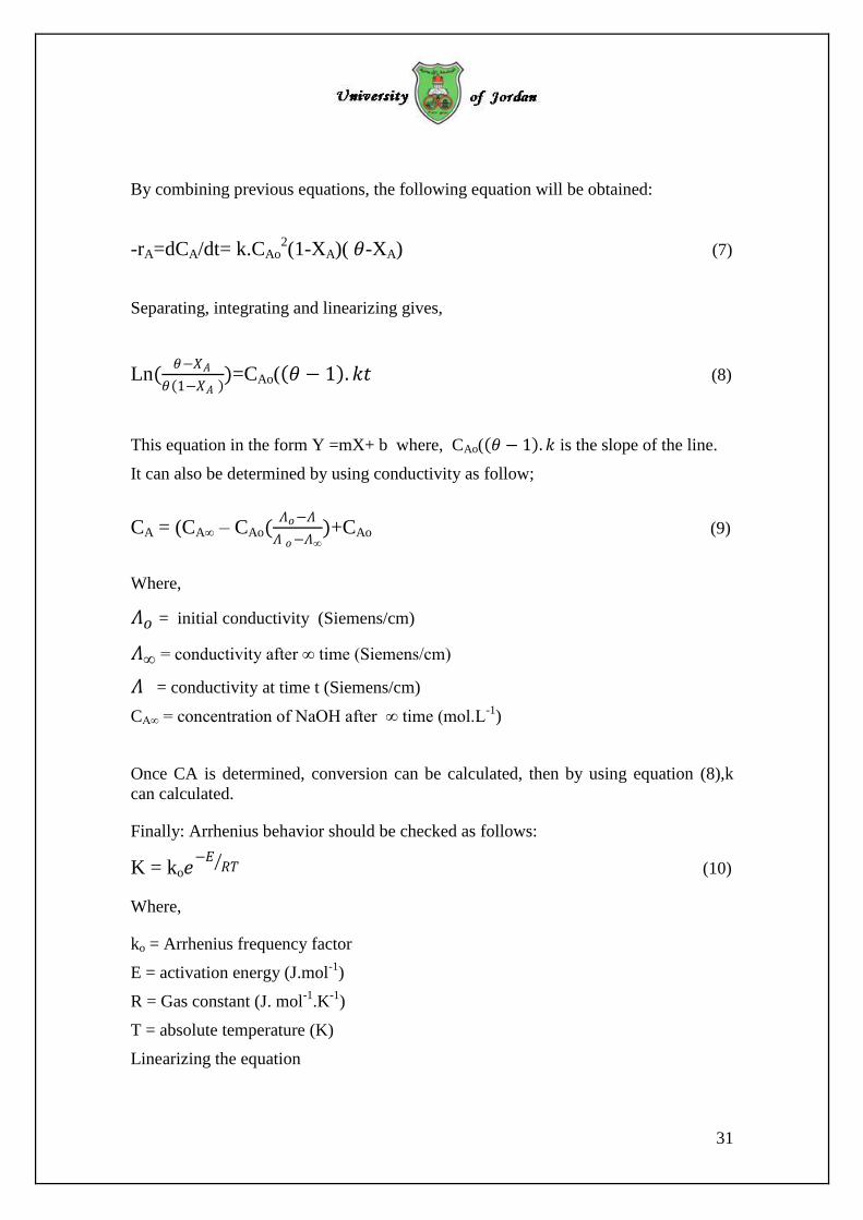
By combining previous equations, the following equation will be obtained:

-rA=dCA/dt= k.CAo2(1-XA)( 𝜃-XA) (7)

Separating, integrating and linearizing gives,

Ln(𝜃−𝑋𝐴

𝜃 1−𝑋𝐴 )=CAo( 𝜃 − 1 . 𝑘𝑡 (8)

This equation in the form Y =mX+ b where, CAo( 𝜃 − 1 . 𝑘 is the slope of the line.

It can also be determined by using conductivity as follow;

CA = (CA∞ – CAo(𝛬𝑜−𝛬

𝛬 𝑜−𝛬∞)+CAo (9)

Where,

𝛬𝑜 = initial conductivity (Siemens/cm)

𝛬∞ = conductivity after ∞ time (Siemens/cm)

𝛬 = conductivity at time t (Siemens/cm)

CA∞ = concentration of NaOH after ∞ time (mol.L-1

)

Once CA is determined, conversion can be calculated, then by using equation (8),k

can calculated.

Finally: Arrhenius behavior should be checked as follows:

K = ko𝑒−𝐸

𝑅𝑇 (10)

Where,

ko = Arrhenius frequency factor

E = activation energy (J.mol-1

)

R = Gas constant (J. mol-1

.K-1

)

T = absolute temperature (K)

Linearizing the equation

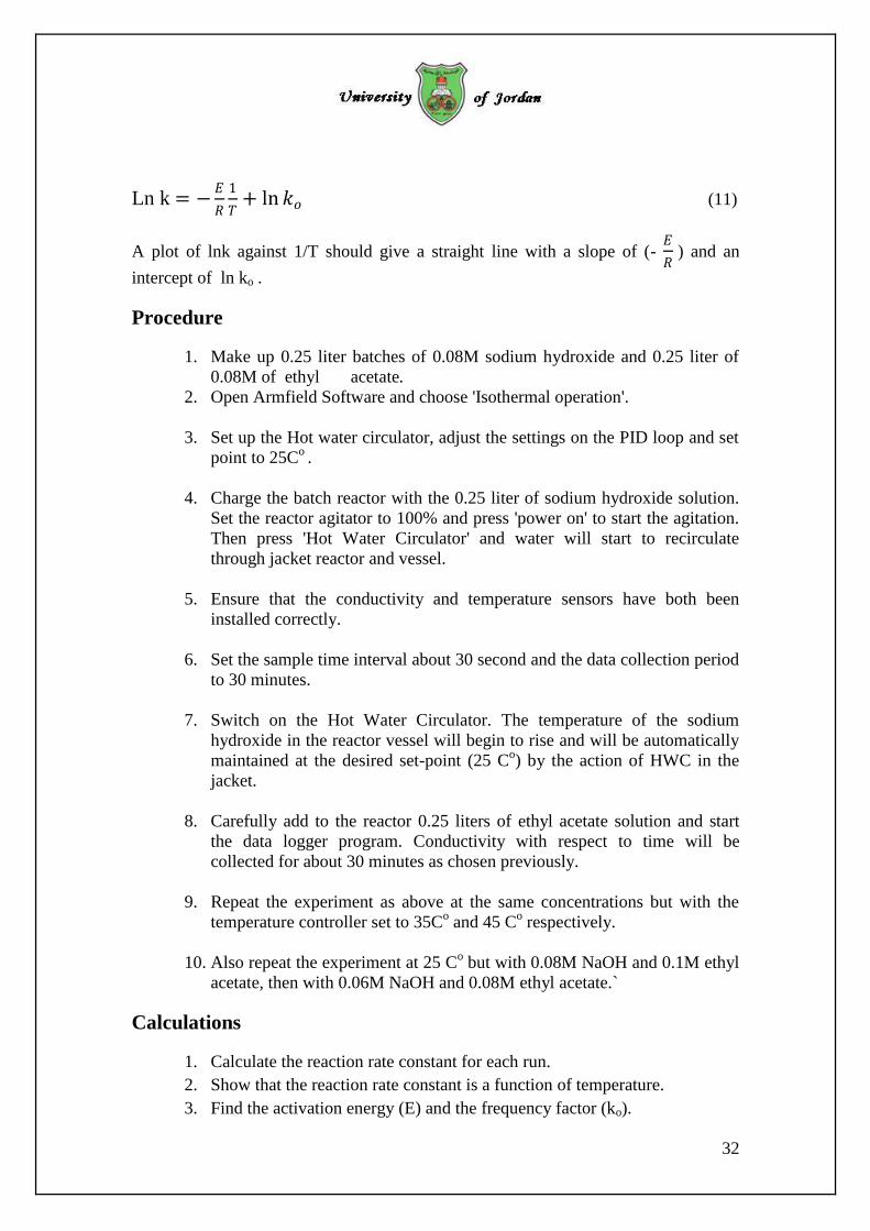
32

Ln k = −𝐸

𝑅

1

𝑇+ ln 𝑘𝑜 (11)

A plot of lnk against 1/T should give a straight line with a slope of (- 𝐸

𝑅 ) and an

intercept of ln ko .

Procedure

1. Make up 0.25 liter batches of 0.08M sodium hydroxide and 0.25 liter of

0.08M of ethyl acetate.

2. Open Armfield Software and choose 'Isothermal operation'.

3. Set up the Hot water circulator, adjust the settings on the PID loop and set

point to 25Co .

4. Charge the batch reactor with the 0.25 liter of sodium hydroxide solution.

Set the reactor agitator to 100% and press 'power on' to start the agitation.

Then press 'Hot Water Circulator' and water will start to recirculate

through jacket reactor and vessel.

5. Ensure that the conductivity and temperature sensors have both been

installed correctly.

6. Set the sample time interval about 30 second and the data collection period

to 30 minutes.

7. Switch on the Hot Water Circulator. The temperature of the sodium

hydroxide in the reactor vessel will begin to rise and will be automatically

maintained at the desired set-point (25 Co) by the action of HWC in the

jacket.

8. Carefully add to the reactor 0.25 liters of ethyl acetate solution and start

the data logger program. Conductivity with respect to time will be

collected for about 30 minutes as chosen previously.

9. Repeat the experiment as above at the same concentrations but with the

temperature controller set to 35Co and 45 C

o respectively.

10. Also repeat the experiment at 25 Co but with 0.08M NaOH and 0.1M ethyl

acetate, then with 0.06M NaOH and 0.08M ethyl acetate.`

Calculations

1. Calculate the reaction rate constant for each run.

2. Show that the reaction rate constant is a function of temperature.

3. Find the activation energy (E) and the frequency factor (ko).

33

References

1. Octave Levenspiel,’’Chemical Reaction Engineering”, Second Edition,

John Wiley and Sons,1972.

2. CEXC Instruction Manual, ISSUE 6, March 2012.

3. CEB-MKIII Instruction Manual, ISSUE 2, December 2011.

34





Tubular Flow Reaction

Experiment (4)

Objective

To determine the order, rate constant and activation energy of the reaction between

ethyl acetate and sodium hydroxide using a tubular reaction.

Apparatus

The Reaction consists of reactor vessel, two flow meters, control panel, heating

element, two pumps, feed tanks, solenoid valve, sump tray, thermometer and sheath.

See fig.(1)

35

Procedure

1. Prepare 10 liters of 0.04 M solution of both caustic soda and ethyl acetate,

place them respectively in tanks A and B.

2. Prepare 2 liters of 0.02 M solution of HCl and 2 liters of 0.01 M solution

of NaOH.

3. Connect the solenoid valve at the back of the unit to the cold water supply

and open cold water valve as well as control valve on solenoid.

4. Connect electrical supply to the unit and switch on the mains. Adjust set

point on temperature controller to 10 Co for almost five minutes then

increase the set point to the required temperature. (Wait until the required

temperature is reached).

5. Switch on the stirrer and both pumps, and then adjust flow rates to low

value. Flow rates of sodium hydroxide and ethyl acetate should be adjusted

to equimolar concentration of the reactants at the inlet of the tubular

reactor.

6. At steady state find the conversion of NaOH.

7. Repeat the experiment at higher flow rates.

8. Use an integral method of analysis to determine the reaction rate constant

assuming that the reaction is second order.

9. Repeat the determination of reaction rate constant at two other

temperatures within approximately 5Co apart and hence determine the

activation energy of the reaction.

Calculation

1. Determine the reaction rate equation ( order and rate constant).

2. Show that the reaction rate constant is a function of temperature.

3. Find the activation energy (E) and the frequency factor( Ko).

References

1. Octave Levenspiel, ’’Chemical Reaction Engineering”, Second Edition,

John Wiley and Sons, 1972.

2. Hovorika, R.B.and Kendall, H.B., Eng. Progr., 54(8), 58(1960).

3. Seader, J.D., and Sonthwick, L.M., Chem.Eng.Commun., P 175-183,

(1981).

36

Item Run1 Run2 Run3 Run4

Ethyl acetate conc. In feed tank

Sodium hydroxide conc. In feed tank

HCl concentration (titrant)

NaOH conc. (titrant)

Flow rate of ethylacetate

Flow rate of ethylacetate

Residence time

Mass of (beaker+15ml of Hcl)

Mass of (beaker+15ml of Hcl+10ml sample)

Volume of NaOH (titrant)

Temperature

Tubular's Data Sheet

37





Development of Kinetic Rate Equation

From Hydraulic Analog Methods

Experiment (5)

Objectives

To develop kinetic rate equation of different reaction types and order in batch reactor

using hydraulic analog methods.

Procedure

1. First order irreversible reaction

1. Connect a glass capillary to a burette as shown in Figure 1.

2. Fill the burette with water.

3. At time zero, let the water flow out and record the change in volume as time

progresses.

This experiment represents first order reaction in a batch reactor in which the volume

readings in burette in cm3

is to be considered as a concentration of reactant in mol/m3.

Volume

(cm3)

Time

(sec)

at start V=50 cm3

horizontal capillary should be

level with the zero volume

reading on the burette

Figure 1. Experimental set up to represent the first order

decomposition of reactant A, A R.

[Type a quote from the document or the summary of an

interesting point. You can position the text box anywhere in

the document. Use the Text Box Tools tab to change the

formatting of the pull quote text box.]

38

Calculations:

Find the rate equation of the analog reactions

A R

-rA = k CAn

, n 1.

2. First order series reaction

1. Set up the arrangement shown in Figure 2.

2. Fill burette A with water.

3. At time zero, let the water flow out of both burettes A and R, and record the

change in volume in both burettes (A and R) as time progress.

Calculations:

The rate of the reaction constants (n,k) should be found for the analog reaction

A R S

k1 k2

A

R

S


decomposition of reactant A, A R S.

39

-rA = k1 CAm

and rS = k2 CRn , m n 1.

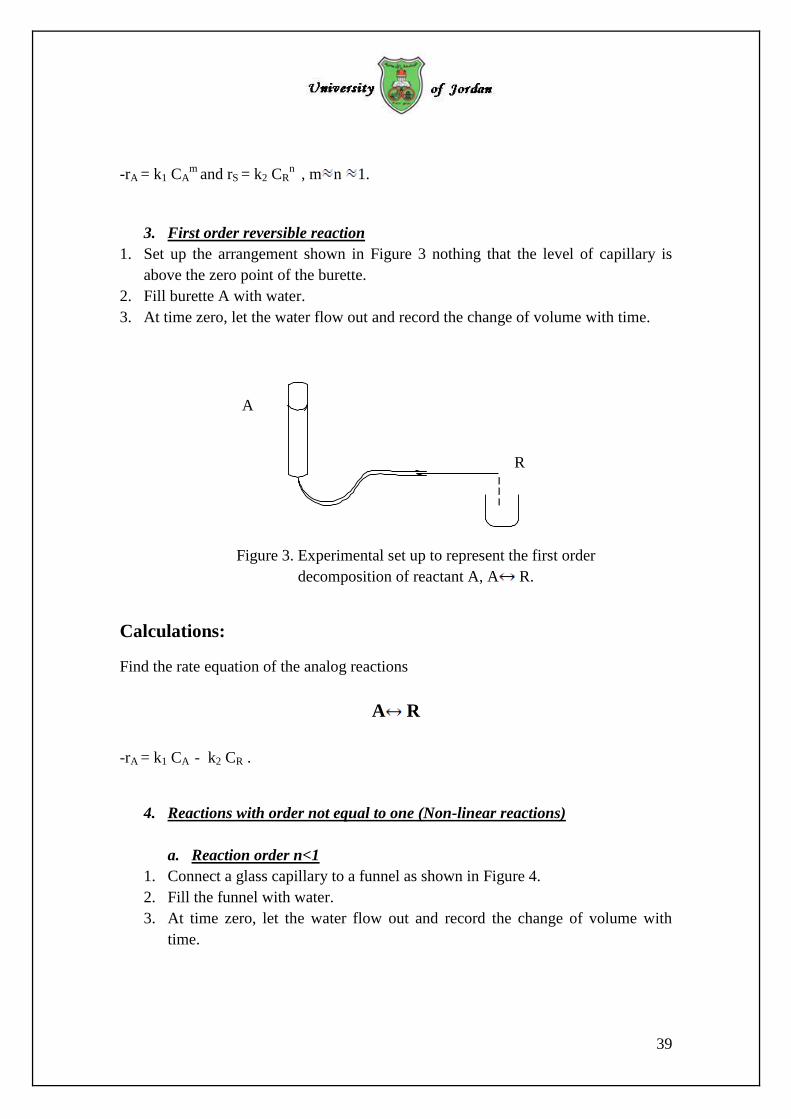
3. First order reversible reaction

1. Set up the arrangement shown in Figure 3 nothing that the level of capillary is

above the zero point of the burette.

2. Fill burette A with water.

3. At time zero, let the water flow out and record the change of volume with time.

Calculations:


A R

-rA = k1 CA - k2 CR .

4. Reactions with order not equal to one (Non-linear reactions)

a. Reaction order n<1

1. Connect a glass capillary to a funnel as shown in Figure 4.

2. Fill the funnel with water.

3. At time zero, let the water flow out and record the change of volume with

time.

A

R


decomposition of reactant A, A R.

40

Calculations:


-rA = k CAn

, n<1

b. Reaction order n>1

1. Set up the arrangement shown in Figure 5.

2. Fill the funnel with water.

3. At time zero, let the water flow out and record the change of volume with

time.

R

L

horizontal capillary should be

level with the bottom of the

container L

A

horizontal capillary should be level

with the vertex of the funnel

Figure 4. Experimental set up to represent the first order decomposition

of reactant A, for non linear rxns n<1.

A

R


decomposition of reactant A, for non linear rxns n>1.

pe a quote from the document or the summary of an

interesting point. You can position the text box anywhere in

the document. Use the Text Box Tools tab to change the

formatting of the pull quote text box.]

41

Calculations:


-rA = k CAn

, n>1

References

Octave Levenspiel, “Chemical Reaction Engineering”, Second Edition, John Wiley

and Sons, 1972.

Guo-Tai and Shan-Drag H. , Chem. Eng. Educ. Winter 1984, p. 10. Spring 1984, p.

64.

42

Hydraulic Analog's data sheet

Time Reaction

Volume

Reaction

Volume

Reaction

Volume

Reaction

Volume

Reaction

Volume

43





Level Control

Experiment (6)

Objectives

1. To become familiar with the coupled tank apparatus.

2. To investigate the steady state and transient performance of the coupled

tank apparatus under proportional and proportional plus integral control.

Introduction

Very often a physical system can be represented by several first order processes

connected in series. Consider the basic coupled tank apparatus. The equations

describing the dynamic behaviour of the system can be derived by considering

flow balances about each tank, assuming that the inter-tank holes and drain tap

behave like orifices. By taking the Laplace transforms of the equations, the

following transfer function is obtained:

)1)(1(

1

)(

)(

21

22

ss

lk

sq

sh

i (1)

Where h 1 is the level in tank 2 and q i is the input flow rate. The time constants τ1

and τ2 are obtained by solving the equations:

21

2

21kk

A ,

21

2121

)2(

kk

kkA (2)

ss HH

gacdk

21

11

12

2

(3)

32

22

22

2

HH

gacdk

s (3’)

44

Where,

A = cross sectional area of either tank 1 or 2.

Cd1,Cd2 = discharge coefficient of the orifice (approx.0.6)

a1 = cross sectional area of orifice 1(the area of the open holes between the two

tanks).

a2 = cross sectional area of orifice 2 (the drain tap).

H1s,H2s = steady state height of fluid in tank 1 and tank 2.

H3 = height of drain tap (3 cm).

The second order transfer function given by eqn.(1) describes the variations in the

input flow rate qi (s). A similar, small signal transfer function can be found which

relates h1(s) -the level of fluid in tank 1- to small variation in the input flow rate

qi(s); It is:

)1)(1()(

)(

21

2121

21

1

ss

skk

A

kk

kk

sq

sh

i (4)

The coupled tank apparatus can be converted to a first order system by removing

all the bungs from the inter-tank partition. This makes a1 in eqn.(3) relatively

large, so that (1/k1) is approximately zero. Using this approximation in Eqn. (1)

gives the small signal transfer function for the coupled tank with all bungs

removed as:

)1(

/1

)(

)( 22

s

k

sq

sh

i (5)

Where τ is given by:

2

2

k

A

(6)

45

Description of Apparatus

The coupled tank apparatus consists of a transparent plexi-glass container

measuring approximately 20 cm by 10 cm deep by 30 cm high. A centre partition

is used to divide the container into two tanks. Flow between the tanks is by means

of a series of holes drilled at the base of the partition. Three holes having

diameters of 1.27 cm, 0.95 cm and 0.635 cm are situated 3 cm above the base of

the tank. A smaller (bleed) hole of 0.317 cm diameter is situated at a height of

1.5cm. These holes constitute orifice 1 of cross sectional area a1. Water is pumped

from a reservoir into the first tank by a variable speed pump which is driven by an

electrical motor. The pump motor drive is normally derived from an analogue

computer. The actual flowrate is measured by a flow meter which is in the flow

line between the pump and tank 1. The depth of the fluid is measured using depth

sensors which are stationed in tank 1 and tank 2. This device performs as an

electrical resistance which varies with the water level. The change in resistance

are detected and provide an electrical signal which is proportional to the height of

water. The water which flows into tank 2 is allowed to drain out via an adjustable

tap, and the entire assembly is mounted in a large tray which also forms the supply

reservoir for the pump. Fully open, the drain tap has a diameter of 0.7cm.

Procedure

1. Measurement of system characteristics

a. Stead State Characteristic of Final Control Element (Pump)

Apply a small positive voltage to the pump drive socket using one of the

potentiometers of the analogue computer, and read off the corresponding

flow rate from the flowmeter. Increase the voltage in increments of about

0.5 volts and record the corresponding flow rates. Continue until the

maximum flowrate is reached.

Requirement: plot the flowrate versus voltage applied to obtain the pump

characteristic (Gp).

b. Steady State Characteristic of Measuring Device (Level Sensor)

Close the drain tap on tank 2 and run the pump until the tanks are both full.

Switch the depth sensor filters in circuit and attach the tank 2 depth output

46

terminal to recorder and record the fluid level in tank 2 and the voltage

reading. Open the drain tap and allow the water level to fall one

centimeter, record the new fluid level and the voltage reading. Repeat the

exercise until the tank is empty.

Requirement: plot the voltage reading versus the fluid level in tank 2 to

obtain the depth sensor characteristics(Gd).

c. Dynamic Characteristics

Open the holes of 0.95 cm and 0.635 cm diameters and close the bleed

hole and hole of 1.27 cm diameter. Open the drain tap fully and run the

pump to give a flowrate of 1850 cc/min and record the steady state

levels(H1s,H2s). Repeat the experiment with another flowrate(2020

cc/min).

Requirements: Determine

gacd 211 , gacd 222

Using the following equations:

gacd 211 = 𝑂𝑖

𝐻1𝑠−𝐻2𝑠

(7)

gacd 222=

𝑄𝑖

𝐻2𝑠−𝐻3 (8)

Derivable from the relationships for the orifices.

Calculate k1 and k2 using Eqn.(3).

Calculate τ1 and τ1 using Eqn. (2).

Evaluate the system transfer functions, Eqn.(1) and (4).

d. Steady State Operating Levels.

Open the drain tap fully and close all except the two holes of 0.635 cm and

0.95 cm diameter. Apply a suitable drive voltage to the pump to obtain a

flowrate of 1000cc/min. allow time for the steady state to be reached and

measure the tank levels H1s and H2s. Repeat the exercise for flow rates of

1850cc/min and 2020cc/min.

Requirement: compare the steady state level in tank 1 predicted by the

equation;

H1s,th = H2s(1+(a2/a1)2)-H3(a2/a1)

2 (9)

with the experimental results.

47

2. Design of Proportional and Integral Controllers

a. Steady State Errors Using Proportional Control

Open the drain tap fully and plug all except the two holes of 0.635 cm and 0.95

cm diameter. Switch the depth sensor filter in circuit. Use the analogue computer

to apply a proportional feedback control loop for the fluid level in tank 2; see

Fig.(1). Set the desired level in tank 2 corresponding to sensor signal of

approximately 6 volts and record the steady state error for constant reference

input and values of proportional gain Kp ranging from 10 to 100.

Requirement: Calculate the theoretical values of the steady state errors using the

equation below and compare them with the experimental ones.

Experimental steady state error:

ess,exp= required level- H2s,exp= Yr-H2s,exp (10)

Theoretical steady state error is calculated from equation:

ess,th= Yr-H2s,th (11)

H2s,th can be evaluated by solving the following equations;

gacd 211 = 𝑂𝑖

𝐻1𝑠,𝑡ℎ−𝐻2𝑠,𝑡ℎ

(12)

H1s,th = H2s,th(1+(a2/a1)2)-H3(a2/a1)

2 (13)

b. Steady State Error Using Proportional Plus Integral controllers

Use the analogue computer to apply proportional plus integral feedback

control to the fluid level in tank 2; see Fig.(2). Set the proportional gain at

a value of 10. Slowly turn up the integral gain at the values of (1, 1.5 and

2) and observe the steady state errors decay to zero.

49

Level Control Data Sheet

Measuring Device calibration:

H2 (cm) H2 (V)

50

Pump calibration:

Flowrate (ml/min) Voltage (V)

51

Proportional Controller:

Set point=

Time Kp = Kp = Kp =

52

Proportional and Integral Controller:

Set point=

Kp =

Time τi = τi = τi =

53

Procedure:

1. Run the SIMULINK module: ResponseHighOrderProcessOpenLoop.mdl to open the above flowsheet.

2. Set = 7, kp = 1 & introduce a unit step change in the load (double click the Step in load icon) and run the SIMULINK model using final simulation

time: 200 units of time.

3. Double click the scope to see the recorded output response.

4. Run the file: FSIMULINKplot.m to plot the recorded output and save the MATLAB figure in a specified directory.

5. Save the excel file: SIMULINKResults.xls to a specified directory if you wish to plot the recorded output using Microsoft excel.

Required:

1. Fit the recorded response to a First-order plus dead time model (FOPD) and estimate its three parameters (kp, td & ) .

2. Compare the response of the FOPD to the original response of the high order process on the same plot.

3. Comment on your results.

( )2

1

pk

st +

( )2

1

pk

st +

( )2

1

pk

st +

54

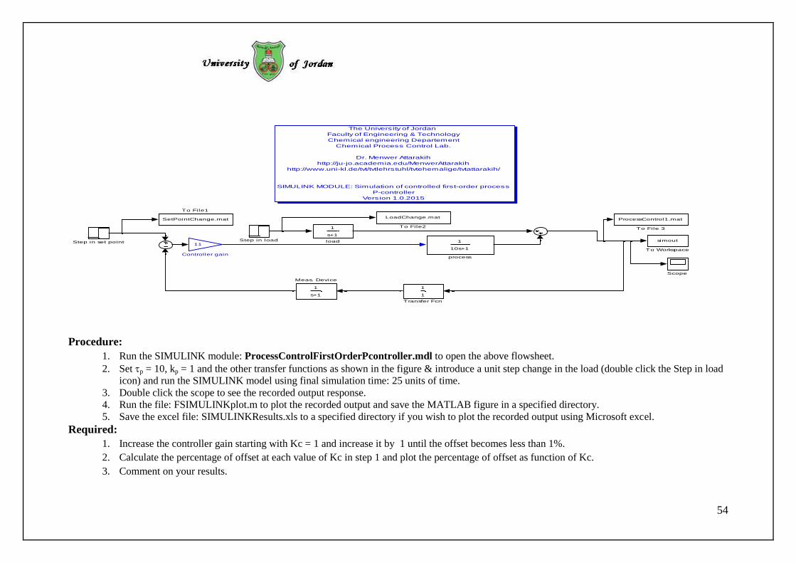
Procedure:

1. Run the SIMULINK module: ProcessControlFirstOrderPcontroller.mdl to open the above flowsheet.

2. Set p = 10, kp = 1 and the other transfer functions as shown in the figure & introduce a unit step change in the load (double click the Step in load

icon) and run the SIMULINK model using final simulation time: 25 units of time.




Required:

1. Increase the controller gain starting with Kc = 1 and increase it by 1 until the offset becomes less than 1%.

2. Calculate the percentage of offset at each value of Kc in step 1 and plot the percentage of offset as function of Kc.

3. Comment on your results.

The University of Jordan

Faculty of Engineering & Technology

Chemical engineering Departement

Chemical Process Control Lab.

Dr. Menwer Attarakih

http://ju-jo.academia.edu/MenwerAttarakih

http://www.uni-kl.de/tvt/tvtlehrstuhl/tvtehemalige/tvtattarakih/

SIMULINK MODULE: Simulation of controlled first-order process

P-controller

Version 1.0.2015

1

10s+1

process

1

s+1

load

1

1

Transfer Fcn

simout

To Workspace

LoadChange.mat

To File2

SetPointChange.mat

To File1

ProcessControl1.mat

To File 3

Step in set pointStep in load

Scope

1

s+1

Meas. Device

11

Controller gain

55

Procedure: 1. Run the SIMULINK module: ProcessControlFirstOrderPIcontroller.mdl to open the above flowsheet.

2. Set p = 10, kp = 1 and the other transfer functions as shown in the figure & introduce a unit step change in the set point(double click the Step in

set point icon) and run the SIMULINK model using final simulation time: 200 units of time.




Required: 1. Did the Integral control action eliminate the offset? Why?

2. At constant I =10.0 increase the controller gain starting with Kc = 1 until the closed loop response oscillates continuously. What is the physical

significance of this controller gain? When the system will become unstable?

3. Repeat step 2 using at least four different integral time constants. Present your results in a table and discuss your results.

4. Repeat step 1 to 3 using only a unit step change in the load.









PI-controller

Version 1.0.2015

1

10s+1

process

1

s+1

loadsimout

To Workspace

LoadChange.mat

To File2SetPointChange.mat

To File1ProcessControl1.mat

To File 3

Step in set point

Step in load

Scope

1

s+1

Meas. Device

10s+1

10s

Integral controller time constant

tau_I = 10.0

11

Controller gain

56

Procedure: 1. Run the SIMULINK module: ProcessControlFirstOrderPIDcontroller.mdl to open the above flowsheet.

2. Set p = 10, kp = 1 and the other transfer functions as shown in the figure & introduce a unit step change in the set point(double click the Step in

set point icon) and run the SIMULINK model using final simulation time: 200 units of time.




Required: 1. What will be the expected effect of the PID controller action?

2. At constant I =10.0 and D =1.5 increase the controller gain starting with Kc = 1 until the closed loop response oscillates continuously. What is

the physical significance of this controller gain? When the system will become unstable?

3. Repeat step 2 using at least four different integral and derivative time constants. Present your results in a table and discuss it.

4. Repeat step 1 to 3 using only a unit step change in the load.

5. With the process under the PI control action at I =10.0 and under continuous oscillation, simulate the closed loop using the PID controller.

Record your observations & discuss the results.









PID-controller

Version 1.0.2015

1

10s+1

process

1

s+1

load

simout

To Workspace

LoadChange.mat

To File2SetPointChange.mat

To File1ProcessControl1.mat

To File 3

Step in set point

Step in load

Scope

1

s+1

Meas. Device

10s+1

10s

Integral controller

tau_I = 0.1

1.5s+1

0.1*1.5s+1

Derivative action

alpha = 0.1

tau_d = 1.5

11

Controller gain

57

Procedure: 1. Run the SIMULINK module: ProcessControlPIDcontrollerSecondOrderWithTimeDelay.mdl to open the above flowsheet.

2. Set p = 7, kp = 4 and the other transfer functions as shown in the figure & introduce a unit step change in the set point(double click the Step in set

point icon) and run the SIMULINK model using final simulation time: 300 units of time.




Required: 6. What will be the expected effect of the dead time (time delay) on the controlled response?

7. At constant I =10.0 and D =2.1 Kc = 0.5 increase the time delay starting with td = 0.25 until the closed loop response oscillates continuously.

What is the physical significance of this behaviour?

8. Repeat step 2 using at least four different integral and derivative time constants. Present your results in a table and discuss it.

9. Repeat steps 1 to 3 using only a unit step change in the load.








SIMULINK MODULE: Simulation of controlled second-order process pluse dead time

PID-controller with dead time simulation

Version 1.0.2015

4

den(s)

process

simout

To Workspace

LoadChange.mat

To File2

SetPointChange.mat

To File1

ProcessControl1.mat

To File 3

Step in set point

Step in load

Scope

1

0.1s+1

Measuring Device

10s+1

10s

Integral action

tau_I = 10

2.1s+1

0.1*2.1s+1

Derivative action

alpha = 0.1

tau_d = 2.1

Dead time

0.5

Controller gain






EMPIRICAL DYNAMIC MODELES

Experiment (8)

Objective: To model a black box process (e.g. continuous stirred tank heater) using the

process step testing method (process reaction curve).


1. Theory:

Empirical (Black box) models do not describe the physical phenomena of the process,

they are based on input/output data and only describe the relationship between the

measured input and output data of the process. These models are useful when limited

time is available for model development and/or when there is insufficient physical

understanding of the process. To generate such empirical models, the step test procedure

is carried out as follows:

1. With the loop is opened ( the controller is on manual mode), apply a step change

in the controller output signal ( )M t to the process (see Fig.(1)). The magnitude of

the change should be large enough for the consequent change in the transmitter

signal to be measurable, but it should not be so large that the response will be

distorted by the process nonlinearities. During the step testing there should be no

disturbances affect the process.

2. The response of the process ( )C t is recorded on a strip chart recorder or

equivalent device, making sure that the resolution is adequate in both the

amplitude and the time scale. The resulting plot of ( )C t versus time has a

sigmodal shape and is known as the process reaction curve. The response must

cover the entire test period from the introduction of the step test until the system

reaches a new steady state.

3. Match the process reaction curve to a FOPDT (First-Order Pluse Dead Time)

response.


Fig.(1): Block diagram for a typical open loop to generate the process reaction curve.

The FOPDT transfer function is given by:

0

( ) .1

t sp

p

K e mC s

s st

-D

=+

(1)

The above equation can be inverted back to the time domain:

0( )

0( ) ( ) 1 p

t t

pC t K m u t t e t

--ِ و

÷ç ÷ç= ´ D ´ - - ÷ç ÷÷çè ّ` (2)

Where 0

( ) ( )C t c t c= - is the output variable in deviation form.

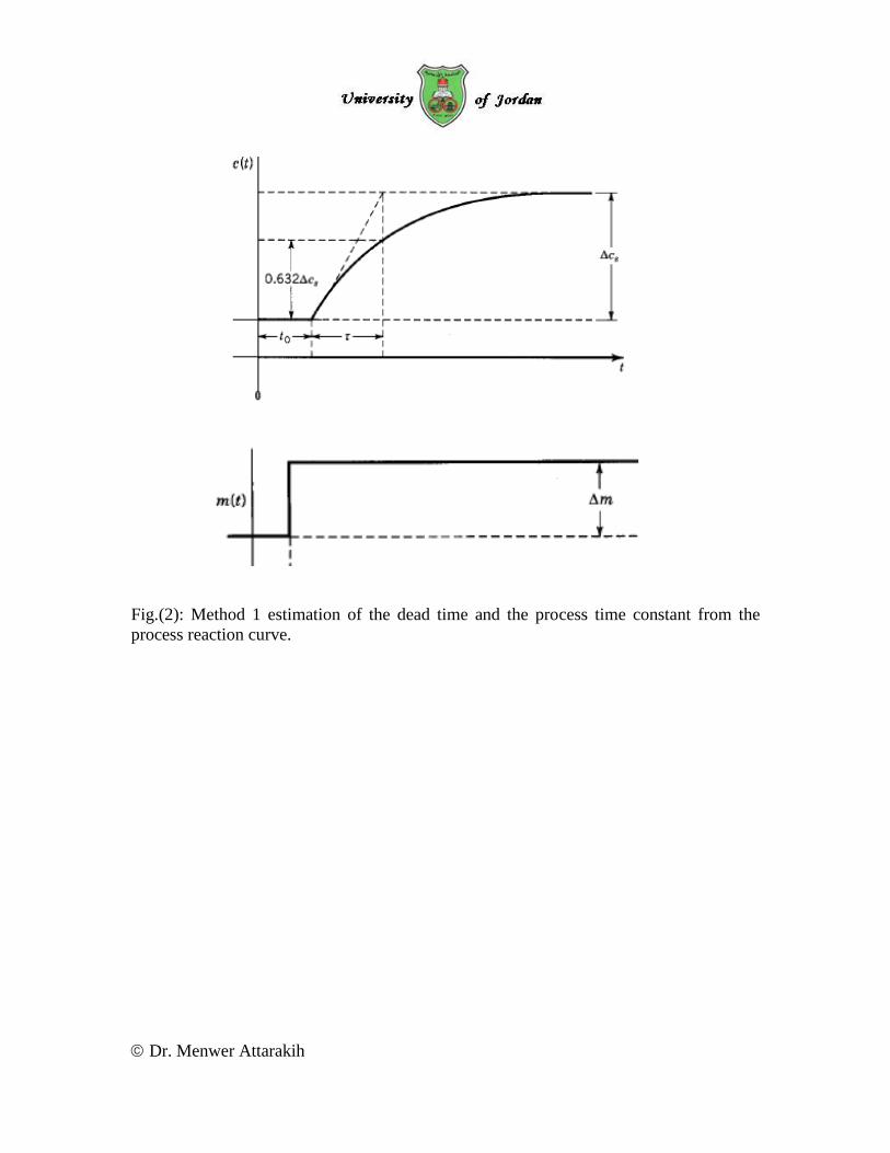
The three model parameters are estimated from the process reaction curve as follows:

pc

Km

D=

D at steady state (3)

The dead time ( 0t ) and the process time constants ( pt ) are estimated from Fig.(2)

below:


Fig.(2): Method 1 estimation of the dead time and the process time constant from the

process reaction curve.


Fig.(3): Method 2 estimation of the dead time and the process time constant from the

process reaction curve.

By using method 2 given in Fig.(3) the process time constant and the dead time are

estimated as follows:

( )2 1

3

2p t tt = - (4)

( )0 2 pt t t= - (5)


Fig.(4): Method 3 estimation of the dead time and the process time constant by drawing

a slope to the process reaction curve passing through the inflection point.

Method 3 uses the inflection point of the process reaction curve to estimate the FOPDT

model parameters as shown in Fig (4).

2. Calculations:

1. Use methods 1, 2 and 3 to estimate the three parameters of the FOPDT model and

list them as shown in table 1:

2. Plot the resulting models using Eq.(2) along with the experimental data on the

same graph.

Table 1: Comparison between different methods for fitting the process reaction

curve to FOPDT model.

Method 1 2 3

pK ( )

0t ( )

pt ( )

3. Comment on the results in (1) and (2).


References:

1. Considine, D. M. (1974). Process instruments and control handbook. McGraw-

Hill, New York.

2. Seborg, D. E. & Edgar, T. F. (1989). Process dynamics and control, John Wiley &

Sons, New York.

chemical engineering laboratory (4) - university of jordanengineering.ju.edu.jo/laboratories/lab4...

Documents