chemical engineering research and designegr.uri.edu/wp-uploads/che/ghceos5.pdfnumerical results for...

Dsc

HD

1

Tsioitfaia

ali

h0

chemical engineering research and design 9 2 ( 2 0 1 4 ) 1977–1991

Contents lists available at ScienceDirect

Chemical Engineering Research and Design

j ourna l h omepage: www.elsev ier .com/ locate /cherd

ensity and phase equilibrium for ice andtructure I hydrates using the Gibbs–Helmholtzonstrained equation of state

eath Henley, Edward Thomas, Angelo Lucia ∗

epartment of Chemical Engineering, University of Rhode Island, Kingston, RI 02881, United States

a b s t r a c t

A new, rigorous framework centered around the multi-scale GHC equation of state is presented for predicting bulk

density and phase equilibrium for light gas–water mixtures at conditions where hexagonal ice and structure I hydrate

phases can exist. The novel aspects of this new framework include (1) the use of internal energies of departure for ice

and empty hydrate respectively to determine densities, (2) contributions to the standard state fugacity of water in ice

and empty hydrate from lattice structure, (3) computation of these structural contributions to standard state fugacity

from compressibility factors and EOS parameters alone, and (4) the direct calculation of gas occupancy from phase

equilibrium. Numerical results for densities and equilibrium for systems involving ice and/or gas hydrates predicted

by this GHC-based framework are compared to predictions of other equations of state, density correlations, and

experimental data where available. Results show that this new GHC-based EOS framework accurately predicts the

densities of hexagonal water ice and structure I gas hydrates as well as phase equilibrium for methane–water and

CO2–water mixtures.© 2014 The Institution of Chemical Engineers. Published by Elsevier B.V. All rights reserved.

Keywords: Hexagonal ice; Methane gas clathrate hydrates; Multi-scale Gibbs–Helmholtz Constrained equation; Lattice

structure contributions to standard state fugacity of water; Gas hydrate occupancy; Structure 1 clathrate hydrates

(3) Deeper locations in permafrost have been suggested as

. Introduction

he general warming of land and oceans around the world haspawned interest in understanding long term environmentalmpacts associated with the melting of ice sheets and thawingf permafrost regions. Permafrost, which accounts for approx-

mately 25% of the land mass in the Northern Hemisphere, ishe general term used to describe land that remains below 0 ◦Cor two or more years at depths that can range from less than

meter to around 1000 m. While temperatures and pressuresn permafrost regions vary, typical ranges are −20 ◦C to 5 ◦Cnd 0.1 to ∼10 MPa, respectively.

Phase behavior in permafrost regions is quite complicatednd can involve light gases (e.g., methane and carbon dioxide),iquid water, brines, hexagonal ice, and gas hydrates – depend-
ng on conditions. Understanding physical property and phase
∗ Corresponding author. Tel.: +1 401 874 2814.E-mail address: [email protected] (A. Lucia).

Available online 20 June 2014ttp://dx.doi.org/10.1016/j.cherd.2014.06.011263-8762/© 2014 The Institution of Chemical Engineers. Published by

behavior in permafrost regions is important for several com-peting reasons:

(1) The large amount of methane sequestered in permafrostis a potential source of low carbon fuel if it can be captured.According to Kvenvolden (1998) there is an estimated2.1 × 1016 standard cubic meters (SCM) of methane con-tained in hydrates on the ocean bottom, which is twicethe energy sum of all other fossil fuels on Earth. Thereis also an estimated 7.4 × 1014 SCM in permafrost regions(see, MacDonald, 1990).

(2) Thawing of permafrost increases microbial activity, whichin turn has the potential to release large amounts of green-house gases (CO2 and methane).

potential sites for carbon storage.

Elsevier B.V. All rights reserved.

http://www.sciencedirect.com/science/journal/02638762

www.elsevier.com/locate/cherd

http://crossmark.crossref.org/dialog/?doi=10.1016/j.cherd.2014.06.011&domain=pdf

mailto:[email protected]

dx.doi.org/10.1016/j.cherd.2014.06.011

1978 chemical engineering research and design 9 2 ( 2 0 1 4 ) 1977–1991

Nomenclature

a, aM pure component energy parameter, energyparameter for liquid mixture

A dimensionless energy parameterb, bi, bM molecular co-volume, pure component molec-

ular co-volume, mixture molecular co-volumeB dimensionless molecular co-volumef, fi fugacity, partial fugacity for component iG Gibbs free energyH enthalpykB Boltzmann constantp, pc pressure, critical pressureq electrostatic charge parameterR universal gas constantS structure parameterT, Tc absolute temperature, critical temperatureUD, UD

i, UD

M internal energy of departure for liquid, inter-nal energy of departure for component i,mixture internal energy of departure

V molar volumexi ith component liquid mole fractionz compressibility factor

Greek symbols� structure parameter, change in variableε well potential energyϕ, ϕi fugacity coefficient, ith component partial

fugacity coefficient� molar densityω acentric factor

Superscriptscalc calculatedD departure functionexp exponential function, experimentalfus fusionhyd hydrateice hexagonal iceig ideal gasL liquidMT empty hydrate0 standard state

Subscriptsc critical propertyi component indexM mixturew water

of cubic equations, only the volume translated equations,

Everyone has an intuitive feel or understanding of ice andhexagonal ice is the only ice that occurs naturally on Earth.As its name implies, 1 h ice has a hexagonal lattice structure.Hydrates, on the other hand, are less well known and under-stood, despite the fact that they were discovered in 1810 (see,Ghiasi, 2012) and later identified as the cause of flow assur-ance problems in gas lines by Hammerschmidt (1934). Gasclathrate hydrates are non-stoichiometric compounds thatoccur at ambient temperature and moderate pressure. Theyare heterogeneous structures that consist of hydrogen bondedwater molecules that form a hydrate lattice stabilized by small
gas molecules called guests (e.g., methane, carbon dioxide,
nitrogen, hydrogen, ethane, etc.). The empty hydrate latticeis not stable on its own. There are three naturally occurringhydrate structures found on Earth – type I (S1), type II (S2)and type H (SH), where the structure is determined by condi-tions of temperature and pressure and the guest molecule(s).Structure 1 hydrates are composed of two 512 cages, six 51262

cages from 46 water molecules. Structure 2 hydrates are com-posed of sixteen 512 cages, eight 51264 cages, and 136 watermolecules. Finally, structure H hydrates consist of three 512

cages, two 435663 cages, and one 51268 cage and have 34 watermolecules. Here the general notation en describes a polygonsuch that has e edges and n faces.

The focus of this work is the modeling of physical prop-erties, specifically density, and phase behavior of mixturesof light gas and water at conditions typically found in per-mafrost regions (i.e., temperatures ranging from 250 to 280 Kand pressures from 0.1 to ∼10 MPa) using an equation ofstate. We show that the multi-scale Gibbs–Helmholtz Con-strained (GHC) equation (Lucia, 2010; Lucia et al., 2012; Luciaand Bonk, 2012), can be used to predict thermo-physical prop-erties and phase equilibrium in systems involving gas, liquid,hexagonal (1 h) ice and gas hydrate. Accordingly, the remain-der of this paper is organized in the following way. Section2 gives a brief survey of relevant literature while Section 3provides some general background information for the multi-scale Gibbs–Helmholtz Constrained (GHC) equation of state.In Section 4, lattice structure considerations in defining thestandard state fugacity of water in an ice phase, NTP MonteCarlo simulations of liquid water, and the Clapeyron equationare used to extend the multi-scale GHC equation to calcu-late densities and phase equilibrium for hexagonal (1 h) ice.A similar extension of the GHC equation that exploits struc-ture in defining the standard state of water in a gas hydratephase is described in Section 5. In Section 6, several numericalexamples that illustrate the accuracy of multi-scale GHC equa-tion predictions of physical properties and phase behavior of1 h ice and gas hydrates. Finally, conclusions of this work aredescribed in Section 7 as well as future work in extending ourapproach to modeling ice and gas hydrates in the presence ofbrines.

2. A brief review of relevant literature

Many traditional equations of state (EOS) have been used tomodel various thermo-physical properties and phase equilib-rium involving mixtures of light gases and water includingthe Soave–Redlich–Kwong (SRK) equation (Soave, 1972), thePeneloux volume translation (Peneloux et al., 1982) of the SRKequation (SRK+), the Peng–Robinson (PR) equation (Peng andRobinson, 1976), the volume translated PR or VTPR equation(Ahlers and Gmehling, 2001), and various forms of the Statis-tical Associating Fluid Theory (SAFT) equation (see Chapmanet al., 1986, 1988, 1989; Kontogeorgis and Folas, 2010). Otherequations of state such as the cubic plus association (CPA)equation (Kontogeorgis et al., 1996; Voutsas et al., 2000) andthe Elliott–Suresh–Donahue (ESD) equation (Elliott et al., 1990)have also been used. There are also specialized equationsof state for water such as the International Association forthe Properties of Water and Steam (or IAPWS-95) equationof Wagner and Pruß (2002), which is formulated in termsof the Helmholtz free energy function. Within the family

SRK+ and VTPR, are capable of predicting reasonably accurate

chemical engineering research and design 9 2 ( 2 0 1 4 ) 1977–1991 1979

d(tamti9tirc

vlatcrptdeup˛

aaIFo2tpocaapd(epmsiam

edtsrStPffprrts

the results are stored in pure component look-up tables

ensities (i.e., AAD% error ≈ 3–4%). See Table 2 in Frey et al.2009) and Table 2 in Ahlers & Gmehling (2001) respec-ively. The CPA, ESD, and SAFT models are much better atpproximating properties and phase equilibrium of water andixtures such as methane–water and CO2–water, etc. because

hey explicitly incorporate association (i.e., hydrogen bonding)n the residual Helmholtz free energy. Finally, the IAPWS-5 equation is the most accurate (∼AAD% error < 0.1%; seehe abstract in Wagner and Pruß, 2002) for water becauset involves a large number of parameters that have beenegressed to a wide range of experimental data; however itannot be used for mixtures.

Equations of state for ice are also available. Within thean der Waals family of cubic equations, there is the trans-ated Trebble–Bishnoi–Salim (TBS) equation of state (Salimnd Trebble, 1994), which is a six-constant EOS for solidshat suffers from the same difficulties that many traditionalubic equations suffer from: (1) excessive use of empiricalelationships to correct deficiencies in the basic theory, (2)oor density predictions without the use of volume transla-ion, and (3) the need to regress parameters to experimentalata. The four primary parameters (a, b, c and d) in the TBSquation must be matched to experimental solid density, sat-ration pressure, and solid and vapor fugacities at the tripleoint. The other two parameters, m and p, are part of the-function for predicting vapor pressure. In addition, temper-ture and pressure-dependent binary interaction parametersre needed for reliable phase equilibrium computation. TheAPWS-95 model for water has been extended to 1 h ice byeistel and Wagner (2006) and uses a Gibbs potential equationf state. Like the model for liquid water (Wagner and Pruß,002), the extended IAPWS-95 equation for 1 h ice has been fito a large amount of experimental data (i.e., 14 independentarameters fit to 522 data points from 32 separate categoriesf experimental data). This experimental data includes spe-ific Gibbs free energy data, specific entropy data, (∂p/∂T) datalong the ice melting curve, heat capacity data, volumetricnd volume-temperature derivative data, isentropic com-ressibility data, and isentropic compressibility-temperatureerivative data. See Table 5 on page 1027 in Feistel and Wagner

2006). As a result, the extended IAPWS-95 equation providesxcellent agreement with experimental values of thermo-hysical properties of hexagonal ice. Other approaches forodeling ice (e.g., Yoon et al., 2002) use a more traditional

olid–liquid equilibrium formulation in which the fugacity ofce is expressed in terms of the fugacity of sub-cooled waternd an exponential correction based on enthalpy and volu-etric differences due to fusion.The most commonly used models for predicting the prop-

rties of gas hydrates are based on the cell theory modeleveloped by van der Waals and Platteeuw (1959) and givenhe acronym vdWP. A detailed derivation of the model fromtatistical mechanics as well as a very good survey of theelevant hydrate literature can be found in the textbook byloan and Koh (2007). Here a brief overview of the modifica-ions of the vdWP model is given starting with the work ofarrish and Prausnitz (1972) who extended the model to allowor the practical calculation of hydrate dissociation pressuresor mixtures of guest molecules. Klauda and Sandler (2000)resented a fugacity-based model that removed the need foreference energy parameters for the empty hydrate lattice andelaxed the incorrect vdWP assumption that the volume ofhe crystal lattice is independent of guest molecule type. A
imilar model was developed by Ballard and Sloan (2002) and
Jager et al. (2003). More recently, Bandyopadhyay and Klauda(2011) presented an updated fugacity model that uses thePRSK equation to represent the fluid phases in equilibriumwith the hydrate. Other modifications include models thataccount for multiple cage occupancy (see, Klauda and Sandler,2003; Martin, 2010), those that correct for contributions tothe Helmholtz free energy due to guest–guest interactions(Zhdanov et al., 2012), and others (e.g., Jäger et al., 2013) thatadapt the model originally developed by Ballard and Sloan(2002) so that highly accurate reference EOS can be used. Thislast approach has also been tested against a large data set forCO2 hydrate. The vdWP model with all of its recent adapta-tions has enjoyed great success and is used heavily in industrybecause of its accuracy and relative simplicity. However, it is asemi-empirical model that requires adjustable parameters tobe regressed to experimental data. For this reason it is difficultto make predictions about the phase behavior and propertiesof potentially hydrate-forming systems outside the ranges ofexperimental data.

3. The multi-scale Gibbs–HelmholtzConstrained (GHC) equation

The multi-scale Gibbs–Helmholtz Constrained (GHC) equation(Lucia, 2010; Lucia et al., 2012; Lucia and Bonk, 2012), which isa modification of the Soave form of the Redlich–Kwong (RK)equation (see Soave, 1972), is given by

p = RT

V − b− a(T, p)

V(V + b)(1)

where p is pressure, T is temperature in Kelvins, V is the molarvolume, R is the universal gas constant and a and b are theenergy and molecular co-volume parameters respectively.

3.1. Pure components

The multi-scale GHC equation is a radically different approachto EOS modeling that is based on three simple ideas:

(1) The molecular co-volume for the liquid, bL, is set equal tothe molar volume of the pure solid or high density (glassy)liquid.

(2) The liquid phase energy parameter, aL(T, p), is constrainedto satisfy the Gibbs–Helmholtz equation, which results inthe following expression for pure liquid components

aL(T, p) =[

a(Tc, pc)Tc

+ bLUDL

Tc ln 2+ 2bLR ln Tc

ln 2

]T − bLUDL

ln 2

−[

bLUDL

ln 2

]T ln T (2)

where Tc is the critical temperature, pc is the criticalpressure, a(Tc, pc) = 0.42748R2T2

c /pc, and UDL is the inter-nal energy of departure for the liquid phase given byUDL = UDL(T, p) = UL(T, p) − Uig(T), where Uig(T) is the idealgas internal energy. Note that UD serves as a natural bridgebetween the molecular and bulk fluid length scales.

(3) The internal energy of departure, UDL, is evaluated usingNTP Monte Carlo simulations, where it is important tonote that MC simulations are performed a priori and that

for use in density and fugacity coefficient calculations.


Molecular scale information in Eq. (2) is what makes theGHC equation a multi-scale equation of state.

3.2. Non-electrolyte mixtures

For non-electrolyte liquid mixtures, the multi-scale GHC equa-tion is

aLM(T, p, x) =

[a(TcM,pcM,x)

TcM+ bL

MUDLM

TcM ln 2+ 2bL

MR ln TcM

ln 2

]T

− bLMUDL

M

ln 2−

[2bL

MR

ln 2

]T ln T (3)

where bLM =

∑xib

Li

and UDLM =

∑xiU

DLM , xi is the liquid mole

fraction of component i, and bLi

and UDLi

are the molecularco-volume and internal energy of departure for the ith pureliquid component. Again a detailed derivation can be found inthe literature (Lucia, 2010; Lucia et al., 2012). Mixture criticalproperties are calculated using Kay’s rules

McM =∑

xiMi for i = 1. . .C (4)

where M is either critical temperature or critical pressure.More detailed information associated with the GHC equa-

tion, its derivation, expressions for pure component andpartial fugacity coefficients, and density and phase equilib-rium predictions for a number of systems including pure liquidwater, water-light gas mixtures, n-alkanes of varying chainlength, and electrolyte solutions can be found in Refs. Lucia(2010) and Lucia et al. (2012).

More recently, Lucia and Henley (2013) have shownthat the GHC equation is thermodynamically consistent bydemonstrating that it satisfies the relationship given byRT(∂ ln f/∂p)T = V.

4. Modeling hexagonal ice using the GHCequation

To model hexagonal ice in the GHC framework, values for bice

and UD,ice are needed along with a means of calculating thepure component fugacity of ice.

4.1. The molecular co-volume and internal energy ofdeparture for ice

Two straightforward but important physical interpretationsare required to apply the multi-scale GHC equation (i.e., Eqs.(1) and (2) with appropriate values of b and UD) to 1 h ice:

(1) In our opinion, the correct value for the molecular co-volume for 1 h ice is the molar volume of liquid water (i.e.,bice = 18.015 cm3/mol) because ice melts under pressure.Other values of molecular co-volume we tried includ-ing values for glassy water (16.363 cm3/mol), low densityamorphous (LDA) ice (19.165 cm3/mol), and high densityamorphous (HDA) ice (15.397 cm3/mol), and very highdensity amorphous (VHDA) ice (14.298 cm3/mol) and allwere found to give poorer predictions of density thanbice = 18.015 cm3/mol.

(2) The internal energy of departure for 1 h ice can be calcu-lated in two different ways:

(a) Using the expression

UD,icew = UD

w + UD,fusw (5)

where UDw is the internal energy of departure for liquid

water (already available from NTP Monte Carlo simu-lation) and U

D,fusw is the internal energy of departure

associated with the fusion of water.(b) By direct NTP Monte Carlo simulations of 1 h ice

using an appropriate potential model (e.g., TIP4P-Ew,TIP4P/Ice, etc.).

These two methods for determining UD,icew are described

and compared in considerable detail in Appendix A.

4.2. A reference state for ice

The fugacity coefficient of 1 h ice must be different from thatof liquid water at phase equilibrium. Appendix B shows thatthe natural log of the fugacity coefficient for hexagonal ice canbe rigorously expressed in the form

ln ϕicew = ln ϕL

w − �ice (6)

where ϕicew and ϕL

w are the fugacity coefficients of 1 h ice andliquid water respectively and �ice is a measure of the impactof long-range structure on the fugacity coefficient of ice and isassumed to be constant. This leads to the following expressionfor the standard state fugacity of ice

f 0,icew = Sicep (7)

where Sice = exp(�ice). We also refer to Sice as a lattice structurecontribution.

We adopt this approach because liquid water and 1 h iceboth have tetrahedral kernels but ice has long-range hexago-nal structure. Furthermore, since ice is a condensed phase, itis not unreasonable to assume that the impact of long-rangestructure to be constant (see Fig. A1). Taking the temperaturederivative of Eq. (6) at constant pressure gives

(∂ ln ϕice

w

∂T

)p

=(

∂ ln ϕLw

∂T

)p

(8)

Thus Eq. (2) is directly applicable for determining the energyparameter for 1 h ice. See Appendix B for a discussion of thefundamental basis for Eqs. (6) and (8).

5. Modeling gas hydrates using the GHCequation

Although the approach for modeling gas hydrates using theGHC equation is similar to that of ice, it involves considerablymore detail. This is because

(1) Gas hydrates are unusual heterogeneous structures so itis not at all clear that the usual mixing rules apply – sincethere is really no mixing taking place.

(2) Empty hydrate cages are not stable.(3) Standard states only apply to pure components.

We start with the idea of estimating the bulk density of an
empty hydrate. Why? The reason is that we need some phys-ically sensible way of estimating the fugacity (or Gibbs free


efstfa

5d

Ttb

b

wd(o1ata

mpAugwi

mt

((

((

hv(−

ahcahe

5

Nmt

nergy) of pure or empty hydrate in order for our frameworkor addressing phase equilibrium to be consistent with clas-ical theory. In order to predict empty hydrate density usinghe GHC equation values of the internal energy of departureor an empty hydrate, UD,MT

w , and molecular co-volume, bhydw ,

re required.

.1. The molecular co-volume and internal energy ofeparture for hydrate

he value of the empty hydrate molecular co-volume is takeno be the same as that of a completely filled hydrate and giveny

hydw = 0.148148bCH4 + 0.851852

�ice, (9)

here bCH4 = 29.614 cm3/mol and where the subscript wenotes water and the superscript hyd represents hydrate. Eq.

9) is derived using simple physics by considering the numberf guest and water molecules in a completely filled structure

hydrate. Using Avogadro’s number and the number of guestnd water molecules, one gets the coefficients (or mole frac-ions) shown in Eq. (9). Note also that Eq. (9) can be used forny guest molecule in a structure 1 hydrate, including CO2.

While it appears that Eq. (9) is the same as the usual linearixing rule for bM, it is not. We interpret Eq. (9) as the high

ressure limit of separable gas and solid phases in a hydrate.dditionally, within the GHC approach to hydrates, Eq. (9) issed for both empty and filled gas hydrates regardless of theas occupancy in the cages. Thus there is no mole fractioneighted average of molecular co-volume for hydrate phases;

t is held fixed at the value given in Eq. (9).Because empty hydrates are not stable, considerable care

ust be taken to get estimates of internal energies of depar-ure UD,MT

w . To do this, we did the following:

1) Placed guest molecules in the hydrate cages.2) Equilibrated the simulations with the guest molecules

present.3) Removed the guest molecules.4) Ran production cycles with restricted volume moves so

that the empty cages would not collapse.

We performed NTP Monte Carlo simulations for emptyydrate using the aforementioned procedure over rele-ant ranges of temperatures (250–280 K) and pressures1–100 bar). Values of UD,MT

w ranged from −4.65 × 105 to 4.58 × 105 cm3 bar/mol.

Note that the same general approach for estimating bhydw

nd UD,MTw can be used for structure II and structure H gas

ydrates by (1) modifying Eq. (9) using the correct molecularo-volume for the guest molecule, (2) using the appropri-te mole fractions for a filled structure II or structure H gasydrate, and (3) performing NTP Monte Carlo simulations formpty structure II and structure H gas hydrates.

.2. Gas hydrate density

ext we developed theory for predicting density for physically
eaningful gas hydrates, which have gas molecules occupying
he cavities or cages. Because gas hydrates are heterogeneous

structures, we calculate the density of an S1 gas hydrate usingthe expression

�hyd = (5.75 + �)�MT

5.75(10)

where � is the fractional occupancy of gas in the hydrate cagesand ranges from 0 to 1, �MT is the empty hydrate density com-puted from the GHC equation (i.e., Eq. (2)), and the quantity5.75 is simply the ratio of water molecules to guest molecules(46/8) in a structure 1 hydrate. Note that Eq. (10) is still anapplication of the multi-scale GHC equation to gas hydratesand, in our opinion, provides a straightforward, yet physicallymeaningful, way of computing hydrate density. Moreover, Eq.(10) covers the full range of gas occupancy; thus the more gasthere is in the cages, the denser the hydrate. At the same time,it avoids many of the complications associated with com-position dependence in determining hydrate properties likefugacity coefficients.

Eq. (10) can also be used to estimate the density of struc-ture II and structure H hydrates by simply replacing the value5.75 with 5.67, which is the ratio of water molecules to guestmolecules per unit cell for both structure II and structure Hhydrates.

5.3. A reference state for pure water in gas hydrate

To calculate a standard state for pure water in a hydratephase we let x

hydw = 1 and use a procedure identical to that

in Appendix B for ice. This leads to the expression

f0,hydw = SiceSMTp (11)

where Sice = exp(�ice) and SMT = exp(�MT). The quantity �MT =ln ϕice

w − ln ϕMTw represents the difference in long range struc-

ture between 1 h ice and empty hydrate and can be interpretedas a second structural contribution. Appendix C gives all of thedetails of the derivation of Eq. (11).

6. Numerical results

In this section, numerical results are presented for densityand phase equilibrium for light gas–water mixtures in regionswhere ice and gas hydrate can form. All numerical results pre-sented in this section use the GHC equation of state (except forcomparisons) and were performed in double precision arith-metic on a Dell Inspiron laptop using the Lahey-Fijitsu LF95FORTRAN compiler. Critical property and other relevant dataare summarized in Appendix D.

6.1. Methane–water mixtures

Methane and water can exhibit a number of differentphase equilibrium – gas–liquid, gas–ice, gas–ice-hydrate, andgas–liquid-hydrate at conditions typical of permafrost.

6.1.1. Methane–water in gas–liquid equilibriumNumerical results for methane–water have been reported byLucia and Henley (2013), compared to experimental data ofServio and Englezos (2002), and are reproduced here for thereader’s convenience in Table 1, which shows that the GHCequation provides reasonable predictions of the solubility of
methane in water at the conditions studied by Servio andEnglezos (2002). Additional density and phase equilibrium


Table 1 – Methane solubility in water predicted by the GHC equation.

T (K) p (bar) xexpCH4

a xGHCCH4

% Error

278.65 35 0.001190 0.001104 7.20280.45 35 0.001102 0.001098 0.36281.55 50 0.001524 0.001379 9.51282.65 50 0.001357 0.001374 1.25283.25 65 0.001720 0.001660 3.49284.35 65 0.001681 0.001653 1.67

AAD% 3.91

a Experimental data taken from Table 1 in Servio and Englezos (2002). J. Chem. Eng. Data 47, 89.

Fig. 1 – Comparison of GHC-predicted density formethane–water mixtures with experimental data.

Fig. 2 – GHC-predicted methane solubility in water.

Table 3 shows melting temperatures of ice predicted by

predictions for the GHC equation are compared to experi-mental data and shown in Figs. 1 and 2. Specifically, GHCEOS density predictions are compared to the 169 experimen-tal density measurements in Joffrion and Eubank in Fig. 1 andrange from 398.15 to 498.15 K and approximately 1 to 120 bar.The comparison in Fig. 1 clearly shows a very good matchof the experimental data with statistics of an AAD% error of1.45% and standard deviation of 2.6%. Fig. 2, on the other hand,shows a comparison of GHC-predicted methane solubility inwater in the VLE region with the experimental data of Servioand Englezos (2002) and Chapoy et al. (2004). The tempera-tures and pressures for the data sets in Fig. 2 are 275–313 Kand 10–180 bar while the GHC-predicted values are shown asunfilled triangles and the dot-dot-dash curves. Note the agree-ment is quite reasonable. Remember the GHC EOS does not usebinary interaction parameters at all while the modeling resultsfor the Valderrama–Patel–Teja (VPT) EOS used in Chapoy et al.require binary interaction parameters.

Table 2 – Density of sub-cooled hexagonal ice.

Temperature (K) Pressure (MPa)

260 0.1013

5

10

270 0.1013

273 0.1013

a Reproduced from Table 11 in Feistel and Wagner (2006).b GHC equation with UD,ice

w calculated using Eqs. (5) and (A1).

6.1.2. Hexagonal ice density and the ice-water meltingcurveBefore studying gas–ice equilibrium and to validate the the-ory developed in Sections 4.1 and 4.2 and Appendix B, wepresent results for the density and ice-water melting curveas predicted by the GHC framework.

Table 2 compares the densities of 1 h ice predicted by themulti-scale GHC equation with those given in Feistel andWagner (p. 1040, Table 11, Feistel and Wagner, 2006) for theextended IAPWS-95 equation over the range of interest in per-mafrost phase behavior. In the comparisons in Table 2, the %error is given by %error = 100|�IAPWS-95 − �GHC|�IAPWS-95, whichclearly shows that the GHC equation captures the increase in1 h ice density with decreasing temperature and that thereis reasonably good agreement between the two EOS models.However, the GHC equation does not show the same sensitiv-ity of ice density to temperature and pressure as the extendedIAPWS-95 equation.

the extended IAPWS-95 and GHC equations as a function of

IAPWS-95a GHCb % Error

918.61 931.31 1.38923.84 931.77 0.85928.96 931.93 0.32917.18 927.48 1.12916.74 926.25 1.04


Table 3 – Melting temperatures of 1 h ice predicted by the extended IAPWS-95 & GHC equations.

Pressure (MPa)a Melting temperature, Tm (K) Tm (K) % Error in Tm

IAPWS-95a GHC

0.1013 273.159 273.151 0.048 0.01542.1453 273 273.042 0.042 0.015415.1355 272 272.041 0.041 0.015127.4942 271 271.093 0.093 0.034339.3133 270 270.189 0.189 0.070050.6633 269 269.320 0.320 0.119061.5996 268 268.493 0.493 0.1840

a Reproduced from Table 19 in Feistel and Wagner, p. 1045, 2006.

Fig. 3 – Melting curve for ice predicted by the IAPWS-95 andGHC equations.

pqipttatmtaTsdm

Note that there is reasonably good agreement among all three

ressure and clearly shows that the two EOS are in gooduantitative agreement. Fig. 3, on the other hand, shows the

ce-water melting curve over a much wider range of tem-erature and pressure for both EOS and, again, shows thathere is good quantitative agreement up to 500 bar. Althoughhere are some differences above 500 bar, those differencesre small. Additionally, the IAPWS-95 EOS uses 14 parame-ers and is actually fit to melting curve data, so it should give

ore accurate results. In contrast, the GHC equation only useswo parameters and, in our opinion, does remarkably wellt predicting the 1 h ice melting curve. Finally, the results inables 2 and 3 and Fig. 3 show that the expression for thetandard state fugacity for water in a hexagonal ice phaseerived in Appendix B is useful in predicting the density and
elting temperature for 1 h ice.
Table 4 – Phase equilibria for 10 mol% methane–90 mol% water

Type of equilibrium

GSE

G/RT −7.885069

Phase 1 1 h ice

Phase 1 fraction 0.899987

Phase 1 composition (0, 1)

Phase 1 density (kg/m3) 926.67

Phase 2 Gas


Phase 2 composition (0.999841, 1.5Phase 2 density (kg/m3) 1.95

6.1.3. Methane gas–ice equilibriumAt low enough temperature and pressure, methane andwater will exhibit gas–solid equilibrium with essentially purephases. However, it is important for the reader to understandthat other equilibrium solutions (e.g., gas–liquid equilib-rium) that satisfy the equality of chemical potential buthave a higher Gibbs free energy can be found for the samespecifications of feed composition, temperature, and pressure.Table 4 presents results for the phase equilibrium of a mixtureof 10 mol% methane and 90 mol% water at 272 K and 1 bar.

At the given temperature, the pressure is too low formethane hydrate to form so this example represents a rea-sonable test of the capability of the multi-scale GHC EOS tofind gas–solid equilibrium. Also note that the correct globalminimum Gibbs free energy solution is methane gas witha very small amount of water vapor in equilibrium with1 h ice (GSE). However, there is also a gas–liquid equilib-rium (GLE) solution with a value of G/RT that is only slightlyhigher than the gas–ice equilibrium solution. It is also possibleto find a gas–liquid–ice (GLSE) equilibrium at these condi-tions with a value of G/RT between that of the GS and GLequilibria and a very small amount of solid (∼3.5 mol%/molfeed).

6.1.4. Methane hydrate densityThe next example gives numerical results for GHC-predicteddensity of empty and filled hydrate and, in doing so, teststhe validity of the theoretical material presented in Sec-tions 5.2 and 5.3 and Appendix C. Empty and filled methanehydrate densities are shown in Table 5 along with a com-parison of the GHC-predicted filled methane hydrate densitywith the analytical expression given in Sloan and Koh (2007)with and without the temperature and pressure dependenceof empty cell volume given by Klauda and Sandler (2000).

methods.

at −1.15 ◦C and 0.1 MPa.

Phase equilibria

GLE

−7.880715Liquid0.900014(3.28 × 10−5, 0.999967)1015.041

Gas0.099986

9 × 10−4) (0.999840, 1.60 × 10−4)1.95


Table 5 – Methane hydrate density from Eq. (10) for � = 1.

T (K) p (bar) �MT (kg/m3) �hyd (kg/m3) �hyd (kg/m3)a �hyd (kg/m3)b

260 50 795.43 918.61 913.79 926.46100 795.74 918.98 913.79 926.60

270 50 788.48 910.59 913.79 924.05100 788.96 911.14 913.79 924.19

280 50 781.51 902.54 913.79 921.55100 781.99 903.09 913.79 921.69

a Analytical expression from Sloan and Koh (2007).b Sloan & Koh expression with Klauda and Sandler (2000) temperature and pressure dependent empty cell volume.

Table 6 – Phase equilibria at approximate quadruple point (272.751 K, 25.624 bar) for GHC equation.

Type of equilibrium Phase equilibria

GLE GSE HSE

G/RT −6.98926 −6.98933 −6.99003Phase 1 Liquid Ice IcePhase 1 fraction 0.860690 0.860058 0.008067Phase 1 composition (0.000804, 0.999196) (0, 1) (0, 1)Phase 1 density (kg/m3) 1014.05 926.39 926.39

Phase 2 Gas Gas HydratePhase 2 fraction 0.139310 0.139942 0.991933Phase 2 composition (0.999989, 1.09 × 10−5) (0.999989, 1.09 × 10−5) (0.140978, 0.859022)Phase 2 density (kg/m3) 19.19 19.19 901.31
Occupancy
6.1.5. The quadruple point for methane–water equilibriumBelow the melting point of ice, the phase equilibrium thatexists is either methane gas–ice or methane hydrate–gas/iceequilibrium. That is, at low pressure, below pressures forwhich hydrate can form, methane gas is in equilibrium with1 h ice. See Table 4 for an example of low pressure GSE. As oneraises the pressure at fixed temperature, methane hydrate willform and gas hydrate will be in equilibrium with gas and/orice – depending on the overall amounts of methane and waterin the system. Above the melting point of ice the equilibriumchanges from gas–liquid to methane hydrate–gas/liquid as afunction of increasing pressure. One of the more challengingtasks in the neighborhood of the ice melting point is predictingthe quadruple point – the temperature and pressure at whichfour phases (ice, methane hydrate, liquid water, and gas) co-exist. Anderson (2004) reports a quadruple point of 272.9 K and25.63 bar. Table 6 gives calculated results for the GHC equa-tion prediction of the quadruple point, which is approximately272.751 K and 25.624 bar.

Because the quadruple point is a singular point, it is verydifficult to compute accurately. However, note that the GHC

Table 7 – Phase equilibria for 13 mol% methane–87 mol% water

Type of equilibrium

GLE

G/RT −7.165528

Phase 1 Liquid


Phase 1 composition (0.000850, 0.999150)


Phase 2 Gas


Phase 2 composition (0.999990, 9.87 × 10−6)


Occupancy

0.9437

prediction of the quadruple point gives all three two-phaseequilibria that have dimensionless Gibbs free energies thatare quite close (i.e., differing by <10−3). Note also the predictedfractional occupancy of the gas in the hydrate phase is 0.9437,which is quite close to the value of occupancy of 0.9461 pre-dicted by the correlation in Parrish and Prausnitz (1972) butless close to the value of occupancy of 0.90 ± 0.01 predicted byGibbs ensemble Monte Carlo simulation (GEMC).

6.1.6. Sub-cooled methane hydrate–ice equilibriumThis last methane–water example in this article is usedto illustrate that phase equilibrium and gas occupancy forconditions away from phase boundaries can be determinedusing the theoretical framework described in Sections 3–5 andAppendices A–C. Consider permafrost conditions for a mix-ture of 13 mol% methane and 87 mol% water at 272 K and27 bar. For the given problem (1) there is an excess amount ofwater, (2) methane hydrate should be in equilibrium with pureice, and (3) the resulting phase equilibrium solution is away
from the phase boundary. Numerical results for this exampleare shown in Table 7.
at −1.15 ◦C and 2.7 MPa.

Phase equilibria

GSE HSE

−7.168280 −7.172040Ice Ice0.870062 0.019111(0, 1) (0, 1)926.70 926.70

Gas Hydrate0.0999865 0.980889(0.999990, 9.81 × 10−6) (0.132198, 0.867802)20.35 893.66

0.8759


Table 8 – Ice-empty hydrate equilibrium at −1.15 ◦C and2.7 MPa.

Type of equilibrium Ice-empty hydrate

G/RT −7.172040Phase 1 IcePhase 1 fraction 0.019111Phase 1 composition (6.99 × 10−5, 0.999930)

Phase 2 HydratePhase 2 fraction 0.980889Phase 2 composition (7.23 × 10−5, 0.999928)

taepiwetcvihcpTai

Iuaottt

hticHTt(

It is important to describe the phase equilibrium compu-ations for this ice–gas hydrate equilibrium flash solution in

bit more detail. The water-to-methane ratio in the feed isqual to 6.6923, well in excess of the value of 5.75 for a com-letely filled methane hydrate. Therefore, if methane hydrate

s one of the equilibrium phases, there should also be excessater and this implies that either liquid water or ice will also

xist. In addition, from Table 7 it is clear that ice should behe phase in equilibrium with methane hydrate at the givenonditions. This is true because the GSE solution has a loweralue of G/RT than that for the VLE solution. Moreover, in anyce–methane hydrate equilibrium, methane is confined to theydrate phase. Thus, defining equilibrium becomes a bit morehallenging since, in theory, there is only a single chemicalotential to use to define conditions of phase equilibrium.his is where the use of structural contributions to the icend empty hydrate standard state fugacities for water becomemportant. To define equilibrium we use the condition that

icew − MT

w = 0 (12)

t is also important to understand that Eq. (12) is singularnless trace amounts of methane are permitted in the icend empty hydrate phases. However, even if trace amountsf methane are present in these phases to avoid singularity,he problem is still so nearly singular that quadratic accelera-ion (see, Eq. (A2), p. 2562 in Lucia and Yang, 2003) is requiredo get convergence to a reasonable tolerance.

To give the reader some appreciation for this last point, weave shown the calculated equilibrium solution to Eq. (12) inhe presence of trace amounts of methane at 272 K and 27 barn Table 8. Using quadratic acceleration, these computationsonverge to the solution shown in Table 8 in 20 iterations.owever, note how very close in composition both phases inable 8 are; both contain less than 0.01 mol% methane. The
wo critical pieces of information that come from solving Eq.12) in this regard are the ice and hydrate phase fractions. From
Table 9 – Phase equilibria for 13 mol% CO2–87 mol% water at −8

Type of equilibrium

GSE LL

G/RT −7.963541 −7.791826

Phase 1 1 h ice Liquid

Phase 1 fraction 0.870256 0.871749

Phase 1 composition (0, 1) (0.002010, 0Phase 1 density (kg/m3) 929.33 1016.81

Phase 2 Gas Liquid

Phase 2 fraction 0.129744 0.128251

Phase 2 composition (0.999992, 8.18 × 10−6) (0.999980, 1Phase 2 density (kg/m3) 21.37 716.35

Occupancy

these phase fractions, it is straightforward to determine themethane occupancy, gas hydrate density (i.e., using Eq. (10)),and corresponding value of G/RT for the hydrate phase – aswell as G/RT for the ice–methane hydrate equilibrium solution.

For this particular example, we also calculated the frac-tional occupancy of methane in the hydrate phase usingGibbs-ensemble Monte Carlo simulations for the purpose ofcomparison. The value obtained from GEMC was 0.89 ± 0.01.Table 7, on the other hand, shows that the calculated fractionaloccupancy using the GHC-based framework developed in thework is 0.8759, whereas the occupancy determined using thecorrelation in Parrish and Prausnitz (1972) is 0.9497. Thus it isclear that the proposed GHC-based framework for gas hydratesgives reliable values of gas occupancy directly from phaseequilibrium.

6.2. Carbon dioxide–water mixture

Like methane–water mixtures, carbon dioxide–water mixturescan exhibit a number of different types of phase equilibria –gas–liquid, liquid–liquid, gas–ice, hydrate–ice, etc.

6.2.1. Gas–liquid equilibriumIn previous work, Lucia et al. (2012) have compared phase equi-librium results for CO2–water predicted by the GHC EOS withthose of the Predictive Soave–Redlich–Kwong (PSRK) equationand the experimental data from Coan and King (1971). Seeexample 6.6 and Fig. 14 in Lucia et al. (2012). In general, bothequations of state are in good agreement with experimentaldata with the GHC equation performing better overall.

6.2.2. Carbon dioxide gas–ice equilibriumCO2–ice equilibrium is straightforward to compute usingthe GHC-based framework developed in this work. However,depending on conditions, there can be many other equilib-ria with values of G/RT that are close to the global minimumvalue of G/RT, as illustrated in Table 9. The presence of manyequilibria makes the prediction of the correct solution quitechallenging.

6.2.3. Carbon dioxide hydrate densityThe density of CO2 hydrate is considerably higher than that ofmethane hydrate due to the fact that CO2 is much heavier thanmethane. However, because CO2 hydrate is also a structure1 hydrate, Eq. (10) can be used to calculate hydrate density.Table 10 compares GHC-predicted CO2 hydrate densities withdensities calculated using the analytical expression given in
Sloan and Koh (2007) with and without the Klauda and Sandler(2000) correction for empty hydrate cell volume.
.15 ◦C and 0.1 MPa.

Phase equilibria

E GLE HSE

−7.934062 −7.963296Liquid 1 h ice0.870573 0.017992

.997990) (6.60 × 10−4, 0.999340) (0, 1)1017.92 929.33

Gas Hydrate0.129427 0.982008

.96 × 10−5) (0.999992, 8.46 × 10−6) (0.132067, 0.867933)21.37 1097.18

0.8749


Table 10 – Carbon dioxide hydrate density from Eq. (10) for � = 1.

T (K) p (bar) �MT (kg/m3) �hyd (kg/m3) �hyd (kg/m3)a �hyd (kg/m3)b

260 20 803.28 1144.57 1114.89 1182.8330 803.46 1144.82 1114.89 1182.54

270 20 796.57 1135.00 1114.89 1182.8650 797.90 1135.31 1114.89 1181.72

280 50 789.73 1125.25 1114.89 1181.7570 789.92 1125.52 1114.89 1180.53

a Analytical expression from Sloan and Koh (2007).b Sloan & Koh expression with Klauda and Sandler (2000) temperature and pressure dependent empty cell volume.

Brewer et al. (1999) report a value of 1100 kg/m3 for thebulk density of CO2 hydrate at −4 ◦C and depths from 1100to 1300 m (pressures ranging from ∼110 to 130 bar). From Note17 in Brewer et al. we can deduce that the fractional gas occu-pancy is 0.9583. For the same conditions of temperature andpressure, the empty hydrate density predicted by the GHCequation is 0.0442967 mol/cm3. Using the gas occupancy fromBrewer et al. (1999), the molecular weight of CO2 hydrate is21.59 g/gmol. From Eq. (10), the actual hydrate density for afractional CO2 occupancy of 0.9583 is 0.051679 mol/cm3, whichwhen multiplied by the molecular weight of the CO2 hydrategives a mass density of 1115.57 kg/m3. This GHC-predictedvalue of CO2 hydrate density represents an error of 1.43%.For the exact same conditions, the analytical expression inSloan and Koh (2007) gives a density of 1101.02 kg/m3 whilethe expression in Sloan and Koh with the Klauda and Sandler(2000) correction for empty hydrate cell volume results in amass density of 1162.25 kg/m3. In our opinion, the 1.43% errorin CO2 hydrate density predicted by the multi-scale GHC equa-tion, which is neither a correlation nor a fit to experimentaldata, is quite accurate.

6.2.4. Phase equilibrium in regions where CO2 hydratescan existOne of the interesting differences between methane hydratesand CO2 hydrates is the presence of liquid CO2 at high pres-sure so we consider an example that would potentially resultin storage of CO2 in a hydrate phase. Let the temperature and
pressure be 269.15 K and 130 bar respectively. At this pressure,CO2 is a liquid and the temperature and pressure are such
Table 11 – Phase equilibria for 13 mol% CO2–87 mol% water at −Type of equilibrium

LLE

G/RT −7.341224

Phase 1 Liquid


Phase 1 composition (0.018762, 0.981238)


Phase 2 Liquid


Phase 2 composition (0.999161, 8.39 × 10−4)


Phase 3

Phase 3 fraction

Phase 3 composition

Phase 3 density (kg/m3)

Occupancy

that hydrate can form. Moreover, Brewer et al. (1999) provideclear experimental evidence that a hydrate phase can formfrom liquid CO2 at high pressures. See Fig. 3 and the associ-ated discussions in Brewer et al. (1999). Finally, for hydrate inequilibrium with fluid phases (and not 1 h ice), the conditionsdefining equilibrium are the equality of chemical potentialsfor CO2 and water in all phases. Numerical results are shownin Table 11, which are consistent with the experimental obser-vations of Brewer et al. (1999), where the authors report thepresence of a mass of flocculant CO2 hydrate along with liquidCO2 and, in their case, seawater. The GHC-estimated freezingpoint depression of water with CO2 solute mole fractions of0.018762 or 0.018782 at an elevated pressure is approximately−3.82 ◦C. Thus the estimated freezing point of the water phaseat 130 bar pressure is 269.32 K, which is very close to 269.15 K.This, in our opinion, explains why the values of G/RT for theLLE and SLE flash solutions in Table 11 are so close. In addition,Brewer et al. state that after some time (17 days), they observedno hydrate present in their experiment – either because thehydrate phase dissolved or because it sank into the surround-ing seawater. The GHC-predicted hydrate density shown inTable 11 is consistent with the hydrate phase sinking in water.Finally, the GHC-predicted density and fractional occupancyagree quite well with the density of 1100 kg/m3 and occupancyof 0.9583 reported in Brewer et al. (1999). The fractional occu-pancy predicted by Parrish and Prausnitz (1972) correlationwas 0.9680.

The numerical aspects associated with computing the
HLLE flash solution in Table 11 are somewhat complicated.Because there are two components and three phases, the
4 ◦C and 13 MPa.

Phase equilibria

SLE HLLE

−7.337202 −7.365097Ice Liquid0.870542 0.873997(0, 1) (0.018782, 0.981218)927.92 1029.03

Liquid Liquid0.129458 0.111677(0.999157, 8.43 × 10−4) (0.999156, 8.44 × 10−4)995.77 995.77

Hydrate0.014326(0.139740, 0.860260)1116.320.9432


sfpe

7

Todtesthtped.bdwamaoi

7i

AgoB

(

(

((

(

tcma

Ai

Imo

i

ii

i

olution is near singular and quadratic acceleration is requiredor reliable convergence. In this example, the HLLE flash com-utations converge to an accuracy of 10−6 in the 2-norm of thequality of chemical potentials in 9 iterations.

. Conclusions

he multi-scale Gibbs–Helmholtz Constrained (GHC) equationf state-based framework has been extended for determiningensities and phase equilibrium in light gas–water mix-ures at conditions where ice and/or hydrates can exist. Thisxtended framework is built around the use of the multi-cale GHC EOS, and the novel ideas that (1) make use ofhe GHC equation to determine densities of ice and emptyydrate, (2) derive and employ structural contributions tohe standard state fugacities of ice and empty hydrate inhase equilibrium, (3) use of only densities and EOS param-ters to determine these structural contributions, and (4)etermine gas occupancy directly from phase equilibrium

A novel theoretical framework was developed and a num-er of examples for mixtures of methane–water and carbonioxide–water at conditions relevant to hydrate formationere presented to show the efficacy of the proposed newpproach. Numerical results clearly show that this extendedulti-scale, GHC-based framework is rigorous and provides

ccurate predictions of densities, phase equilibrium, and gasccupancy for light gas–water mixtures for conditions where

ce and/or gas hydrates exist.

.1. Extensions of ice and gas hydrate modeling tonclude brines

s noted in Section 1, permafrost and other regions containingas hydrates can also contain brines. However, the presencef brines further complicates fluid modeling in many ways.rines

1) Increase the internal energy of departure and molecularco-volume of an aqueous electrolyte solution in compar-ison to pure water and thus increase the density of theaqueous liquid phase.

2) Directly affect the fugacity of gases in the aqueous phase,generally lowering their solubility by a process known assalting out.

3) Affect the fugacity of water in the aqueous phase.4) Result in freezing point depression, generally causing a

shift in phase boundaries.5) Generally lower the heat of fusion of water.

Moreover, these factors are all strongly interrelated, effecthe formation/dissociation of gas hydrates, and require veryareful study. In future work, we show how to extend theulti-scale GHC EOS framework for systems that exhibit ice

nd gas hydrates presented in this article to include brines.

ppendix A. Internal energies of departure force

nternal energies of departure for hexagonal ice can be deter-
ined either from UD for liquid water plus energies of fusion
r by direct Monte Carlo simulation.

Internal energies of departure for hexagonal ice fromenergies of fusion

Along the melting curve, internal energies of departure asso-ciated with fusion, U

D,fusw , needed in Eq. (5) can be calculated

as follows:

i. A reference value of the internal energy of departure asso-ciated with fusion, U

D0,fusw , can be estimated from data for

the heat of fusion for water, which is abundantly avail-able (at 273.15 K and 0.1013 MPa; U

D0,fusw = −0.600890325 ×

105 cm3 bar/mol).i. The effect of temperature and pressure on U

D,fusw along the

melting curve can be included by using the Clapeyron equa-tion (see Smith et al., 2004) in the form

UD,fusw = U

D0,fusw + V

[(∂p

∂T

)T + p

](A1)

where V = Vicew − VL

w, (∂p/∂T) is the derivative of pressurewith respect to temperature along the melting curve, andT = T − 273.15.

i. It is straightforward to calculate a very good estimate ofthe volume difference between 1 h ice and liquid water, V,needed in Eq. (A1) using the multi-scale GHC equation. Todo this,(a) First calculate the density of liquid water at 273.15 K

and 0.1013 MPa using the GHC equation with val-ues of bL

w = 16.363 cm3/mol and UDLw = −4.820981356 ×

105 cm3 bar/mol, which is the value of UD for liq-uid water from NTP Monte Carlo simulations. Thecalculated molar density of liquid water is �L

w =0.0563139 mol/cm3, which corresponds to a mass den-sity of 1014.49 kg/m3.

(b) Next set UD,fusw = U

D0,fusw and calculate UD,ice

w = UDLw +

UD,fusw at 273.15 K and 0.1013 MPa. This gives a value of

UD,icew = −5.4218889 × 105 cm3 bar/mol.

(c) Calculate the density of 1 h ice at 273.15 K and0.1013 MPa using the GHC equation (i.e., Eqs. (1) and (2))with bice

w = 18.015 cm3/mol and UD,icew = −5.4218889 ×

105 cm3 bar/mol, which gives a molar density of �icew =

0.05414412 mol/cm3 or a mass density of 926.19 kg/m3.(d) Finally, use the results from (a) and (c) to cal-

culate a value of V = Vicew − VL

w = (1/�icew ) − (1/�L

w) =1.69311 cm3/mol.

v. Given the reference internal energy of fusion, UD0,fusw , and

the change in volume, V, it is straightforward to use theCalpeyron equation to estimate the derivative, (∂p/∂T),along the melting curve at the reference temperature andpressure. By direct application of the Clapeyron equationwe have

(∂p

∂T

)= H

D0,fusw

TV= U

D0,fusw

TV(A2)

which holds since the term pV is negligible compared toU

D0,fusw . From Eq. (A2), we find that (∂p/∂T) =

(−0.600890325 × 105 cm3 bar/mol)/((273.15 K)(1.69311 cm3/mol)) = −129.902 bar/K, which is close tothe published experimental value of –134.58 bar/K foundin the open literature. See, for example, Table IV in Abascalet al. (2005) or p. 1034 in Feistel and Wagner (2006).

v. To calculate UD,fusw at other T and p along the melting

curve, use Eq. (A1) with the assumption that V and


Fig. A1 – Comparison of minimized and simulated
structures of hexagonal.
(∂p/∂T) remain constant at values of V = 1.69311 cm3/moland (∂p/∂T) = −129.902 bar/K respectively.

Internal energies of departure for hexagonal ice fromdirect Monte Carlo simulation

We have also calculated internal energies of departure for 1 hice using the TIP4P-Ew force field model initialized from ahexagonal structure. The optimized force field parameters forliquid water used in the MC simulations of ice were taken fromHorn et al. (2004) and are given in Appendix D. Fig. A1 givesa snapshot of the crystal structure predicted by Monte Carlosimulation for N = 96 water molecules, T = 272 K and p = 10 MPaduring the sampling (or production) phase. For these sim-ulations, 50,000 equilibration cycles and 200,000 productioncycles were used. The minimum energy structure for hexago-nal ice at 0 K is also shown in Fig. A1 for comparison.

Note that the minimum energy structure (at 0 K) is perfectlyhexagonal while NTP Monte Carlo simulation using TIP4P-Ewgives a structure that shows some lattice distortion at theelevated temperature of 272 K. Similar results were obtainedusing the TIP4P/Ice force field model (Abascal et al., 2004).The important point here is that NTP Monte Carlo simula-tions account for the effects of lattice distortion and this latticedistortion is correctly reflected in values of UD,ice

w .It is also important to note that the estimation of UD for

hexagonal ice from direct NTP Monte Carlo simulation is notrestricted to the melting curve but can be used for any tem-perature and pressure. However, it is unclear if this distinctionmatters in practice since Table A1, which gives a comparisonof UD,ice

w calculated using energies of fusion and the Clapeyron
equation (i.e., Eqs. (A1) and (A2)) with values of UD,ice
w calcu-lated from direct NTP Monte Carlo simulations, shows only

Table A1 – Internal energies of departure for hexagonal ice.

T (K) p (MPa) UD,icew

UDLw + U

D,fusw

260 0.1 −5.45437

5 −5.48108

10 −5.47443

270 0.1 −5.43590

5 −5.42835

10 −5.42557

280 0.1 −5.39142

5 −5.38874

10 −5.38620

a Force field model = TIP4P-Ew.

relatively small differences in UD,icew between the two methods

over reasonable ranges of temperature and pressure.The results in Table A1 show that there is strong agree-

ment between the two methods for determining internalenergies of departure for hexagonal ice. Specifically, the %error, which is defined as % error = 100|UD,ice

w (MC) − (UDLw +

UD,fusw )/UD,ice

w (MC)|, is less than 3% and the standard deviation,�N, is small – despite the fact that estimations of UD,ice

w usingthe Clapeyron equation are really not strictly applicable at con-ditions that are not on the melting curve. Note that Table A1also shows that the pressure effect on UD,ice

w is small. We useUD,ice

w = UDLw + U

D,fusw because (1) we already have an extensive

database of UDLw using TIP4P-Ew and (2) UD,ice

w = UDLw + U

D,fusw

provides internal energies of departure that are in good agree-ment with those computed using TIP4P/ice.

Appendix B. A reference state for water in ahexagonal ice phase

The expression for ln � in the multi-scale GHC framework fora pure component is

ln ϕ = z–1– ln(z–B)–(

A

B

)ln

(1 + B

z

)(B1)

where A = ap/R2T2and B = bp/RT. Application of Eq. (B1) to 1 hice and liquid water gives

ln ϕicew = zice

w − 1 − ln(zicew − Bice

w ) −(

Aicew

Bicew

)ln

(1 + Bice

w

zicew

)(B2)

ln ϕLw = zL

w − 1 − ln(zLw − BL

w) −(

ALw

BLw

)ln

(1 + BL

w

zLw

)(B3)

Subtracting Eq. (B2) from Eq. (B3) and some algebra gives

�ice = ln ϕLw − ln ϕice

w = zLw − zice

w − ln(zLw − BL

w) + ln(zicew − Bice

w )

−(

ALw

BLw

)ln

(1 + BL

w

zLw

)+

(Aice

w

Bicew

)ln

(1 + Bice

w

zicew

)(B4)

where �ice denotes the difference between the natural log ofthe fugacity coefficients for water and 1 h ice due to long-range structural differences between water and ice. Note thatEq. (B4) is a rigorous relationship between ln ϕice

w and ln ϕLw

and permits the calculation of the difference between the twofugacity coefficients from information that is readily available

(105 cm3 bar/mol) % Error

NTP MCa 2�N

−5.60955 203.7649 2.77−5.61205 536.3299 2.33−5.61080 224.7205 2.43

−5.57666 207.6345 2.52−5.57490 359.8061 2.63−5.59308 335.1859 2.99

−5.53664 430.5228 2.62−5.54026 362.6037 2.73−5.54201 150.2200 2.81


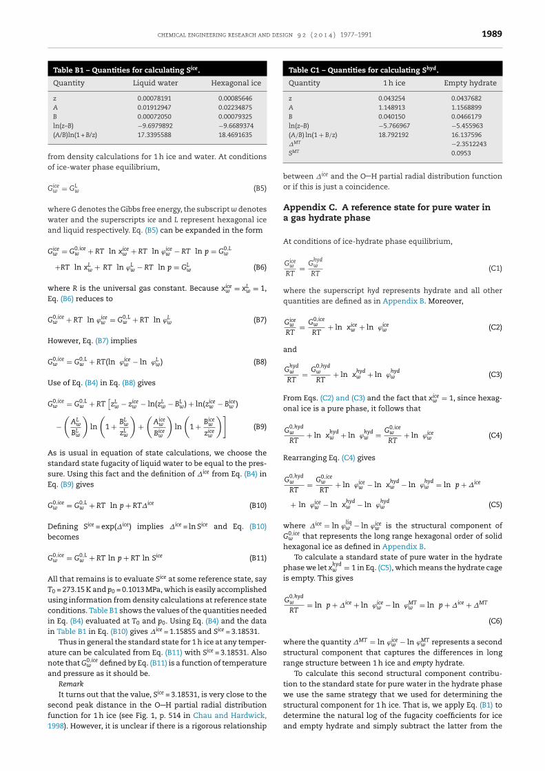
Table B1 – Quantities for calculating Sice.

Quantity Liquid water Hexagonal ice

z 0.00078191 0.00085646A 0.01912947 0.02234875B 0.00072050 0.00079325ln(z–B) −9.6979892 −9.6689374

fo

G

wwa

G

wE

G

H

G

U

G

AssE

G

Db

G

ATucii

ana

sf1

Table C1 – Quantities for calculating Shyd.

Quantity 1 h ice Empty hydrate

z 0.043254 0.0437682A 1.148913 1.1568899B 0.040150 0.0466179ln(z–B) −5.766967 −5.455963(A/B) ln(1 + B/z) 18.792192 16.137596�MT −2.3512243

MT

(A/B)ln(1 + B/z) 17.3395588 18.4691635

rom density calculations for 1 h ice and water. At conditionsf ice-water phase equilibrium,

icew = GL

w (B5)

here G denotes the Gibbs free energy, the subscript w denotesater and the superscripts ice and L represent hexagonal ice

nd liquid respectively. Eq. (B5) can be expanded in the form

icew = G0,ice

w + RT ln xicew + RT ln ϕice

w − RT ln p = G0,Lw

+RT ln xLw + RT ln ϕL

w − RT ln p = GLw (B6)

here R is the universal gas constant. Because xicew = xL

w = 1,q. (B6) reduces to

0,icew + RT ln ϕice

w = G0,Lw + RT ln ϕL

w (B7)

owever, Eq. (B7) implies

0,icew = G0,L

w + RT(ln ϕicew − ln ϕL

w) (B8)

se of Eq. (B4) in Eq. (B8) gives

0,icew = G0,L

w + RT[zL

w − zicew − ln(zL

w − BLw) + ln(zice

w − Bicew )

−(

ALw

BLw

)ln

(1 + BL

w

zLw

)+

(Aice

w

Bicew

)ln

(1 + Bice

w

zicew

)](B9)

s is usual in equation of state calculations, we choose thetandard state fugacity of liquid water to be equal to the pres-ure. Using this fact and the definition of �ice from Eq. (B4) inq. (B9) gives

0,icew = G0,L

w + RT ln p + RT�ice (B10)

efining Sice = exp(�ice) implies �ice = ln Sice and Eq. (B10)ecomes

0,icew = G0,L

w + RT ln p + RT ln Sice (B11)

ll that remains is to evaluate Sice at some reference state, say

0 = 273.15 K and p0 = 0.1013 MPa, which is easily accomplishedsing information from density calculations at reference stateonditions. Table B1 shows the values of the quantities neededn Eq. (B4) evaluated at T0 and p0. Using Eq. (B4) and the datan Table B1 in Eq. (B10) gives �ice = 1.15855 and Sice = 3.18531.

Thus in general the standard state for 1 h ice at any temper-ture can be calculated from Eq. (B11) with Sice = 3.18531. Alsoote that G0,ice

w defined by Eq. (B11) is a function of temperaturend pressure as it should be.

RemarkIt turns out that the value, Sice = 3.18531, is very close to the

econd peak distance in the O H partial radial distribution
unction for 1 h ice (see Fig. 1, p. 514 in Chau and Hardwick,998). However, it is unclear if there is a rigorous relationship
S 0.0953

between �ice and the O H partial radial distribution functionor if this is just a coincidence.

Appendix C. A reference state for pure water ina gas hydrate phase

At conditions of ice-hydrate phase equilibrium,

Gicew

RT= G

hydw

RT(C1)

where the superscript hyd represents hydrate and all otherquantities are defined as in Appendix B. Moreover,

Gicew

RT= G0,ice

w

RT+ ln xice

w + ln ϕicew (C2)

and

Ghydw

RT= G

0,hydw

RT+ ln x

hydw + ln ϕ

hydw (C3)

From Eqs. (C2) and (C3) and the fact that xicew = 1, since hexag-

onal ice is a pure phase, it follows that

G0,hydw

RT+ ln x

hydw + ln ϕ

hydw = G0,ice

w

RT+ ln ϕice

w (C4)

Rearranging Eq. (C4) gives

G0,hydw

RT= G0,ice

w

RT+ ln ϕice

w − ln xhydw − ln ϕ

hydw = ln p + �ice

+ ln ϕicew − ln x

hydw − ln ϕ

hydw (C5)

where �ice = ln ϕliqw − ln ϕice

w is the structural component ofG0,ice

w that represents the long range hexagonal order of solidhexagonal ice as defined in Appendix B.

To calculate a standard state of pure water in the hydratephase we let x

hydw = 1 in Eq. (C5), which means the hydrate cage

is empty. This gives

G0,hydw

RT= ln p + �ice + ln ϕice

w − ln ϕMTw = ln p + �ice + �MT

(C6)

where the quantity �MT = ln ϕicew − ln ϕMT

w represents a secondstructural component that captures the differences in longrange structure between 1 h ice and empty hydrate.

To calculate this second structural component contribu-tion to the standard state for pure water in the hydrate phasewe use the same strategy that we used for determining thestructural component for 1 h ice. That is, we apply Eq. (B1) to
determine the natural log of the fugacity coefficients for iceand empty hydrate and simply subtract the latter from the


Table D1 – Critical and other physical property data.

Species Tc (K) pc (MPa) ω b (cm3/mol)

Methane 190.58 4.592 0.008 29.614Water 647.37 22.120 0.345 16.363Carbon dioxide 304.20 73.80 0.224 28.169

Table D2 – NTP Monte Carlo simulation parameters.

ε/kB (K) � (Å) q (e) Reference

TIP4P-ew Horn et al. (2004)O 81.8989 3.16435 −1.0484H 0.0 0.0 0.5242TraPPE-UA Martin and Siepmann (1998)CH4 148.0 3.73 0.0EPM Harris and Yung (1995)C 28.999 2.785 0.6645O 82.997 3.064 −0.33225

former to get �MT in terms of compressibility and equation ofstate parameters, A and B. The resulting expression for �MT is

�MT = zice − zMT − ln(zice − Bice) + ln(zMT − BMT)

−(

Aice

Bice

)ln

(1 + Bice

zice

)+

(AMT

BMT

)ln

(1 + BMT

zMT

)(C7)

which clearly shows that only EOS information is needed todetermine �MT. Straightforward computations using the GHCequation of state shows that �MT varies very little with tem-perature and pressure (i.e., values of between −2.51 and −2.21over the temperature and pressure ranges shown in Table 1).Table C1 gives a sample calculation of �MT at 270 K and 50 bar.

G0,hydw = RT(ln p + ln Sice + ln SMT) (C8)

where Sice = exp(�ice) = 3.18531 and where SMT = exp(�MT) isallowed to vary with �MT computed by Eq. (C7). However, it isimportant to note that the value of SMT is a very weak functionof pressure in the range 250–280 K.

We also repeated the same derivation of the structuralcomponent for empty hydrate by using water as the referencecondition. Specifically, we re-wrote Eq. (C5) as

G0,hydw

RT= G0

w

RT+ ln ϕ

liqw − ln x

hydw − ln ϕ

hydw

= ln p + ln ϕliqw − ln ϕMT

w = ln p + �MT (C9)

where �MT = ln ϕliqw − ln ϕMT

w now measures the structuralcontribution to the hydrate standard state with respect to pureliquid water. This, in turn, led to an expression very similar toEq. (C7). That is,

�MT = zliq − zMT − ln(zliq − Bliq) + ln(zMT − Bhyd)

−(

Aliq

Bliq

)ln

(1 + Bliq

zliq

)+

(AMT

BMT

)ln

(1 + BMT

zMT

)(C10)

However, this choice for the expression for �MT did not yieldgood results.

Appendix D. Critical and other relevantphysical property data

Critical properties and Monte Carlo simulation parame-ters for the chemical species in this work are shown inTables D1 and D2 respectively.

References

Abascal, J.L.F., Sanz, E., Garcia Fernandez, R., Vega, C., 2005. Apotential model for the study of ices and amorphous water:TIP4P/Ice. J. Chem. Phys. 122 (234511), 1–9.

Ahlers, J., Gmehling, J., 2001. Development of a universal groupcontribution equation of state. 1. Prediction of liquid densitiesfor pure compounds with a volume translated Peng–Robinsonequation of state. Fluid Phase Equilib. 191, 177–188.

Anderson, G.K., 2004. Enthalpy of dissociation and hydrationnumber of methane hydrate from the Clapeyron equation. J.Chem. Thermodyn. 36, 1119–1127.

Ballard, A.L., Sloan, E.D.S., 2002. The next generation of hydrateprediction. I. Hydrate standard states and incorporation ofspectroscopy. Fluid Phase Equilib. 197, 371–383.

Bandyopadhyay, A.A., Klauda, J.B., 2011. Gas hydrate structureand pressure predictions based on an updated fugacity-basedmodel with the PSRK equation of state. Ind. Eng. Chem. Res.50 (1), 148–157.

Brewer, P.G., Friederich, G., Peltzer, E.T., Orr, F.M., 1999. Directexperiments on the ocean disposal of fossil fuel CO2. Science284, 943–945.

Chau, P.-L., Hardwick, A.J., 1998. A new order parameter fortetrahedral configurations. Mol. Phys. 93 (3), 511–519.

Chapman, W.G., Gubbins, K.E., Joslin, C.G., Gray, C.G., 1986.Theory and simulation of associating liquid mixtures. FluidPhase Equilib. 29, 337–346.

Chapman, W.G., Jackson, G., Gubbins, K.E., 1988. Phase equilibriaof associating fluids: chain molecules with multiple bondingsites. Mol. Phys. 65, 1057–1079.

Chapman, W.G., Gubbins, K.E., Jackson, G., Radosz, M., 1989.SAFT: equation of state solution model for associating fluids.Fluid Phase Equilib. 52, 31–38.

Chapoy, A., Mohammadi, A.H., Richon, D., Tohidi, B., 2004. Gassolubility measurement and modeling for methane–waterand methane–ethane–n-butane–water at low temperatureconditions. Fluid Phase Equilib. 220, 113–121.

Coan, C.R., King, A.D., 1971. Solubility of water in compressedcarbon dioxide, nitrous oxide, and ethane. Evidence of
hydration of carbon dioxide and nitrous oxide in the gasphase. J. Am. Chem. Soc. 93, 1857–1862.
http://refhub.elsevier.com/S0263-8762(14)00268-8/sbref0005
































































































































































































































































































































































E

F

F

G

H

H

H

J

J

J

K

K

K

K

K

L

L

lliott, J.R., Suresh, S.J., Donohue, M.A., 1990. A simple equation ofstate for non-spherical and associating molecules. Ind. Eng.Chem. Res. 29, 1476–1485.

eistel, R., Wagner, W.A., 2006. A new equation of state for H2Oice 1 h. J. Phys. Chem. Ref. Data 35, 1021–1047.

rey, K., Modell, M., Tester, J., 2009. Density- andtemperature-dependent volume translation for the SRK EOS.1. Pure fluids. Fluid Phase Equilib. 279, 56–63.

hiasi, M.M., 2012. Initial estimation of hydrate formationtemperature of sweet natural gases based on new empiricalcorrelation. J. Nat. Gas Chem. 21 (5), 508–512.

ammerschmidt, E.G., 1934. Formation of gas hydrates in naturalgas transmission lines. Ind. Eng. Chem. Fundam. 26, 851–855.

arris, J.G., Yung, K.H., 1995. Carbon dioxide’s liquid–vaporcoexistence curve and critical properties as predicted by asimple molecular model. J. Phys. Chem. 99, 12021–12024.

orn, H.W., Swope, W.C., Pitera, J.W., Madura, J.D., Dick, T.J., Hura,G.L., Head-Gordon, T., 2004. Development of an improvedfour-site water model for biomolecular simulations: TIP4P-Ew.J. Chem. Phys. 120, 9665–9678.

ager, M.D., Ballard, A.L., Sloan, E.D., 2003. The next generation ofhydrate prediction. Fluid Phase Equilib. 211 (1), 85–107.

äger, A., Vins, V., Gernert, J., Span, R., Hruby, J., 2013. Phaseequilibria with hydrate formation in H2O + CO2 mixturesmodeled with reference equations of state. Fluid PhaseEquilib. 338, 100–113.

offrion, L.L., Eubank, P.T., 1989. Compressibility factors, densities,and residual thermodynamic properties for methane–watermixtures. J. Chem. Eng. Data 34, 215–220.

lauda, J.B., Sandler, S.I., 2000. A fugacity model for gas hydratephase equilibria. Ind. Eng. Chem. Res. 39, 3377–3386.

lauda, J.B., Sandler, S.I., 2003. Phase behavior of clathratehydrates: a model for single and multiple gas componenthydrates. Chem. Eng. Sci. 58, 27–41.

ontogeorgis, G.M., Folas, G.K., 2010. Thermodynamic Models forIndustrial Applications: From Classical and Advanced MixingRules to Association Theories. John Wiley & Sons, Ltd.,London, UK.

ontogeorgis, G.M., Voustas, E.C., Yakounis, I.V., Tassios, D.P.,1996. An equation of state for associating fluids. Ind. Eng.Chem. Res. 35, 4310–4318.

venvolden, K.A., 1998. Estimates of the methane content ofworldwide gas-hydrate deposits. In: Proceedings of theInternational Symposium of Japan National Oil Company,Methane Hydrates: Resources in the near Future? PanelDiscussion Proceedings, Chiba City, Japan, October 20–22,1998. Japan National Oil Company, Tokyo, Japan, p. 1.

ucia, A., 2010. A multi-scale Gibbs–Helmholtz Constrained cubicequation of state. J. Thermodyn., Article id: 238365,10 pages.

ucia, A., Bonk, B.M., Waterman, R.R., Roy, A., 2012. A multi-scale
framework for multi-phase equilibrium flash. Comput. Chem.Eng. 36, 79–98.
Lucia, A., Bonk, B.M., 2012. Molecular geometry effects and theGibbs–Helmholtz Constrained equation of state. Comput.Chem. Eng. 37, 1–14.

Lucia, A., Henley, H., 2013. Thermodynamic consistency of themulti-scale Gibbs–Helmholtz Constrained equation of state.Chem. Eng. Res. Des. 91, 1748–1759.

Lucia, A., Yang, F., 2003. Multivariable terrain methods. AIChE J.49, 2553–2563.

MacDonald, G.J., 1990. The future of methane as an energyresource. Annu. Rev. Energy 15, 53–83.

Martin, A., 2010. A simplified van der Waals-Platteeuw model ofclathrate hydrates with multiple occupancy of cavities. J.Phys. Chem. B 114 (29), 9602–9607.

Martin, M.G., Siepmann, J.I., 1998. Transferable potentials forphase equilibria. 1. United-atom description of n-alkanes. J.Phys. Chem. B 102, 2569–2577.

Parrish, W.R., Prausnitz, J.M., 1972. Dissociation pressures of gashydrates formed by gas mixtures. Ind. Eng. Chem. Proc. Des.Dev. 11, 26–35.

Peneloux, A., Rauzy, E., Freze, R., 1982. A consistent correction forRedlich–Kwong–Soave volumes. Fluid Phase Equilib. 8, 7–23.

Peng, D.Y., Robinson, D.B., 1976. A new two-constant equation ofstate. Ind. Eng. Chem. Fundam. 15, 59–64.

Salim, P.H., Trebble, M.A., 1994. Modeling of solid phases inthermodynamic calculations via translation of a cubicequation of state at the triple point. Fluid Phase Equilib. 93,75–99.

Servio, P., Englezos, P., 2002. Measurement of Dissolved Methanein Water in Equilibrium with Its Hydrate. J. Chem. Eng. Data47, 87–90.

Sloan, E.D., Koh, C.A., 2007. Clathrate Hydrates of Natural Gases,3rd ed. CRC Press, Boca Raton, FL.

Smith, J.M., van Ness, H.C., Abbott, M.M., 2004. ChemicalEngineering Thermodynamics, 7th ed. McGraw-Hill, NewYork.

Soave, G., 1972. Equilibrium constants from a modifiedRedlich–Kwong equation of state. Chem. Eng. Sci. 27,1197–1203.

van der Waals, J.H., Platteeuw, J.C., 1959. Clathrate solutions. Adv.Chem. Phys. 2, 1–5.

Voutsas, E.C., Boulougouris, G.C., Economou, I.G., Tassios, D.P.,2000. Water/hydrocarbon phase equilibria using thethermodynamic perturbation theory. Ind. Eng. Chem. Res. 39,797–804.

Wagner, W.A., Pruß, A., 2002. The IAPW formulation 1995 for thethermodynamic properties of ordinary water substance forgeneral scientific use. J. Phys. Chem. Ref. Data 31, 387–535.

Yoon, J.H., Chun, M.K., Lee, H., 2002. Generalized model forpredicting phase behavior of clathrate hydrate. AIChE J. 48,1317–1330.

Zhdanov, R., Subbotin, O., Chen, L.-J., Belosludov, V., 2012.Theoretical description of methane hydrate equilibrium in a
wide range of temperature and pressure. Int. J. Comput.Mater. Sci. Eng. 1 (2), 1250017.




































































































































































































































































































































































































































































































































































































































































































































































































































































































































































chemical engineering research and designegr.uri.edu/wp-uploads/che/ghceos5.pdfnumerical results for...

Documents