CHEMICAL GEOLOGY

INCLUDING

ISOTOPE GEOSCIENCE ELSEVIER Chemical Geology 161 (I 999) 415-442

www .elsevier.com 1 locate I chemgeo

Transient redox regimes in a shallow alluvial aquifer

Armand R. Groffman * , Laura 1. Crossey Depanment of Earth and Planetwy Sciences, Nonhrup Hall, Unit·ersity of New Mexico, Albuquerque, NM 87106, USA

Received 20 April 1998; accepted 17 December 1998

Abstract

Using dialysis cells, sediment analysis and systematic ground water sampling we are investigating transient redox gradients in a shallow aquifer at the Rio Calaveras research site located in the Jemez Mountains of northern New Mexico. Hydrochemical data show that the dominant redox potentials shift spatially and temporally from 0 2/H 20 2 during spring to a Fe3 + jFe2 +, Mn4 + /Mn2 + and SOJ- jHS- system with the onset of summer. In autumn, both iron and sulfate reduction processes are more pronounced in the upper meter of the water table a condition that persists until spring snow melt infiltration. Infiltration of spring snow melt transports dissolved oxygen to the top of the aquifer where it reacts with Fe2 + and HS- and shifts the redox potentials from moderately reducing to moderately oxidizing in the upper regions of the aquifer. Redox is strongly controlled by inputs of organic carbon, the primary reductant in the system. Low molecular weight organic acids (acetate, formate, propionate and oxalate) are vertically zoned with a greater abundance in the upper meter of the aquifer. Organic acids, derived from organic-rich sediments in the aquifer, are transported from the overlying vadose zone reservoir providing a substrate for heterotrophic bacteria that reduce the terminal electron acceptors (TEAs) 0 2 , Mn02(s)• Fe(OH)3(s) and soJ-. We postulate that two central mechanisms are primarily responsible for transient redox gradients during an annual cycle: (I) bacterially mediated reduction of manganese, iron and sulfate shifts redox to moderately reducing conditions during autumn and (2) transport of molecular oxygen to the top of the water table during infiltration events oxidizes Fe2+ and HS- diminishing their concentrations and shifting redox towards more oxidizing conditions. © 1999 Elsevier Science B.V. All rights reserved.

Keywords: Ground water; Redox gradients; Redox processes; Terminal electron accepting processes; Biogeochemistry

I. Introduction

Oxidation-reduction (redox) gradients in ground water systems are typically viewed as a sequence of spatially distributed discrete zones each dominated

• Corresponding author. E-mail: groffman@unm.edu

by a master electrochemical couple which controls the dominant potential (Back and Barnes, 1965; Baedecker and Back, 1979; Champ et al., 1979; Chapelle, 1993). Thermodynamically, the sequence of potentials determined by redox couples, i.e., 0 2 /H 2 0 2 , NO:J jNO;-, Mn4 + /Mn2+, Fe3+ jFe2 +,

SOi- /HS- and C 4 + /C 4- define a redox ladder

(Berner, 1981) descending from high (oxidizing) to low (reducing) potentials at specific tiers or steps in pH-Eh space (Langmuir, 1997). This creates a

0009-25411991$ - see front matter © 1999 Elsevier Science B.V. All rights reserved. PIJ: S 0 0 0 9-2 54 I ( 9 9) 0 0 I I 9-9

SEP 2 3 2003

11111111111111111111/111111111 3637

416 A.R. Grojjinan, L.J. Crossey /Chemical Geology 161 (/999) 415-442

somewhat stable and predictable redox gradient in the aquifer from near surface relatively oxidizing conditions to more reducing ground water at depth along a flow path. Microbially-mediated reactions control the distribution of redox determining species, gradients and interfaces in ground water (Vroblesky and Chapelle, 1994; Lovley and Chapelle, 1995).

Much attention has focused on redox gradients in regional ground water systems where residence times are long, flow paths are truncated, and ground water generally flows from oxidized recharge zones to deeper relatively isolated regions of the aquifer where reducing conditions prevail (Back, 1966; Champ et a!., 1979; Chapelle, 1993; Chapelle and Lovley, 1990; McMahon, 1990). However, redox gradients within small scale local flow systems have not been studied as intensely. Local flow systems, characteris­tic of many mountain catchments, contain aquifers that are usually unconfined with ground water recharge occurring at local topographic highs and discharging at local topographic lows (Toth, 1963). Ground water residence times are short and veloci­ties are generally high in this environment. Shallow ground water in local flow systems is susceptible to influences from processes such as atmospheric ex­change (chemical and physical) and imports from biological processes occurring at the land's surface. Inputs include oxidation from atmospheric oxygen (02(aq/H 20 2 ) and reducing compounds, predomi­nantly in the form of organic carbon (dissolved and particulate) from the soil or vadose zone and aquifer sediments. As a result of episodic inputs, the redox regime in ground water is destabilized and the bal­ance of oxidative (OXC) and reductive capacities (RDC) (see Scott and Morgan, 1990) fluctuate. This causes both temporal and spatial migration of redox gradients in the aquifer. Select redox domains in these systems may be superimposed and stratified depending upon the spatial position relative to the flux of inputs and their temporal position in the annual cycle of infiltration events.

This research focuses on transient redox gradients with two important questions: ( 1) are transient redox gradients controlled by the annual cycle of infiltra­tion, i.e., snow melt and summer precipitation and (2) what are the most influential geochemical com­ponents that modify or 'drive' the shift in redox potentials? In order to address these questions we are

investigating a shallow alluvial aquifer located at the Rio Calaveras research site in the Jemez mountains of northern New Mexico. This site is appropriate because it receives pulse precipitation as both winter snow and summer rain and responds with a fluctua­tion in ground water hydrogeochemistry. In addition to observed geochemical data, the relative electron level analysis of Scott and Morgan (1990) is used to detennine the balance of oxidizing to reducing aque­ous species with respect to oxidizing and reducing potential through space and time. Our data suggest­ing that redox gradients are transient and are con­trolled by annual imports of reducing and oxidizing constituents to the aquifer. By focusing on the tem­poral and spatial distribution of terminal electron acceptors (TEAs), electron sources (reductants), and the corresponding redox gradients in the alluvial aquifer, we hope to provide a foundation for further investigations of how redox influences the distribu­tion and mobility of trace elements and contaminants in ground water.

1.1. Measurement of redox gradients

An accurate depiction of redox distribution in natural systems depends upon the ground water mea­surement technique and spatial scale. Traditional methods consist of pumping ground water from an integrated screen interval to the surface where redox is then measured. Redox potentials from this large integrated (mixed) region generally do not represent the various subregions. This is because, chemically and hydraulically heterogeneous sediments contain micro scale diffusion dominated environments (milli­meter to centimeter) that may have a greater degree of equilibrium then ambient advection dominated macro scale environments (1-10m). For example, in environments characterized by low hydraulic con­ductivity with long residence and reaction times, chemical equilibrium may exist. In environments characterized by high conductivity and short resi­dence times disequilibrium may prevail. In order address these problems, we measured redox at a high resolution, using dialysis cells that passively equili­brate with ground water in narrow layers of the aquifer. This allows measurements from discrete sed­iment horizons without mixing pore fluids from dif­ferent environments.

A.R. Grof/inan, L.J. Crossey /Chemical Geology 161 (1999) 415-442 417

1.2. Site description

The Rio Calaveras research site is located approx­imately 3 km northwest of the Valles Caldera in the Jemez Mountains of northern New Mexico at an elevation of 2475 m (Fig. I). A first order stream with a gradient of I .3% drains an area of approxi­mately 37.6 km2 (Wroblicky et a!., 1998). The re­search site is located in a narrow valley topographi-

4

440

•x_.: Hill Slope

TR -I• Stream Transect Wells

X• Shallow Well

MLS-3• Multilevel sampling Well

... · · · · · · Hill Slope Boundary

~ GW Flow Paths

Meters 480 520

Fig. I. Location map of the Rio Calaveras research site showing the distribution of the major sampling wells.

cally bound by steep hill slopes occasionally grading into vertical cliffs. Regional bedrock is composed of nonwelded to densely welded rhyolitic ash-flow de­posits of the Otowi member of the Quaternary Ban­delier Tuff (Smith et a!., I970; Goff et a!., 1988). Valley floor sediments comprise 2-3 m of poorly sorted colluvial wedges, extending out from the val­ley margins, interlayered with fluvial material (90% sand I 0% silt) that together form a matrix-supported aquifer stmcture. Aquifer material is slightly to mod­erately weathered with copious iron staining at and above the water table.

Two perennial springs (Fig. I) and a series of ephemeral springs located along the western valley margin recharge the stream and shallow alluvial aquifer. These springs are very responsive to sea­sonal precipitation especially during spring snow melt when spring flow increases. The stream hydro­graph also rises at this time as a response to in­creased spring flow and local catchment mn off. Horizontal hydraulic conductivity in the alluvium determined from slug injection tests ranges from 3.4 X 10-4 mjday to 7.4 mjday with a geometric mean of 5.3 X 10- 2 mjday and porosity ranges from 39-60% (Wroblicky, I995).

The aquifer at the Rio Calaveras site is recharged by springs and the stream. Surface/ ground water exchange occurs in the near stream subsurface envi­ronment, hyporheic zone, and at select locations stream water recharges ground water in the upper regions of the water table (Valett et a!., I996; Mor­rice, 1997). The hyporheic zone is defined as ground water containing a minimum of I 0% surface water (Triska et a!., 1989). The redox regime in the near stream environment is influenced by the biogeo­chemical character of surface water and biological communities present along ground water recharging flow paths (Morrice, I997; Baker, 1998). Away from the influence of the stream, the redox structure is generally more stable unless affected by the modify­ing effects of rain and snow infiltration events.

Weather data have been collected from a meteoro­logical station located at the Seven Springs fish hatchery approximately 1 mile to the east from June 1995 until August I996 and on site from August 1996 until October I997. On site precipitation recorded during these intervals was 279 mm (1996) and 258 mm (1997). Rainfall occurs during the

418 A.R. Groffinan, L.J. Crossey /Chemical Geology 161 (1999) 415-442

summer months from seasonal monsoon convective thunderstorms and in winter snow accumulates up to I m deep providing ample water storage for infiltra­tion into the subsurface. Snow residence time is related to slope aspect and vegetation pattems. As a response to atmospheric precipitation events, pulse infiltration through the subsurface occurs during spring snow melt and major summer rainfall events. Infiltration pulses modifY ground water chemistry by transporting nutrients, especially organic carbon (Baker, 1998), TEAs, redox reaction products and other solutes, from vadose and atmospheric reser­voirs into the aquifer where they have profound biogeochemical implications. Depending upon the amount of snow fall and the temperature regime, infiltration events may occur as spring snow melt from February to May and summer precipitation from June through October.

2. Methods

2.1. Instrumentation

The Rio Calaveras site currently has over 200 wells and piezometers, 1I suction lysimeters, two stream weirs, and a meteorological station. In order to capture the lateral and vertical hydrochemical structure of ground water, two types of monitor wells were utilized. The first type consists of shallow 5 em. interior diameter (ID) polyvinyl chloride (PVC) wells with 50 em screens placed in the upper water table (approximately 0.5-I.S m deep). The shallow wells, shown in Fig. 1, are positioned in transects across the streamjhyporheic zone and at select loca­tions in the flood plain away from the stream. Sys­tematic monitoring of these wells has been ongoing since 1995. The second type consists of 5 em ID PVC continuously screened wells that penetrate the alluvial sediment up to 3 m. These wells are situated along ground water flow paths and at locations with distinctive sediment characteristics., i.e., high or­ganic carbon and ferric iron content. These wells, the multi level sampling (MLS) series (Fig. 1), are used to study vertical hydrogeochemical structure of the alluvial aquifer and have been systematically moni­tored for the past year using diffusion type multilevel samplers described below.

2.2. Sampling

Shallow wells situated at the top of the water table were sampled using a peristaltic Geo Pump attached to a 4-m length of Tygon© tubing. At least three bore volumes of stagnant well water were purged before collection of ground water samples (Barcelona et al., 1985). Deep wells were sampled using a multilevel sampler designed by Margan M.L.S. The sampler is comprised of a solid polyvinyl chloride (PVC) rod fitted with 13 ml volume cylin­drical diffusion cells capped with 0.2 1-Llll nylon membranes. The cells were isolated in the well casing with neoprene seals at a 12 em resolution. Initially, the cells were filled with deionized water and then allowed to equilibrate with ambient ground water solute; equilibration times detennined with a Br tracer range from seven to II days.

In-line filtration was performed using a 47 mm Gelman filter assembly fitted with a millipore 0.45 t-Llll cellulose membrane. Approximately 40 ml of sample were collected for metal and anion analysis. Samples for metals analysis were preserved in the field with concentrated HN03 to a pH below 2 and anions were kept at 4°C until analysis. Alkalinity samples were collected in 40 ml VOA bottles fitted with a Teflon septum with no head space and kept at 4°C until analysis.

2.3. Field measurements

Water levels, dissolved oxygen (DO), pH, oxida­tion reduction potential (ORP), and temperature (T) were measured in the field. Water levels were mea­sured monthly with a Heron Dipper-T well sounder. Dissolved oxygen was measured down hole with a YSI 55B DO meter equipped with ultra sensitive membranes and calibrated at the beginning of each sampling round.

Down hole DO was measured before samples were collected on shallow and fully screened multi­level sampling wells. The analytical detection limit for the YSI 55B is approximately 0.4 mgjl (400 ppb) DO (YSI instrument manual). Only one mea­surement was recorded for the shallow lateral wells and multiple measurements were taken first at 6 em below the phreatic surface then at 15 em increments from top to bottom on the deep MLS wells.

A.R. Groffinan, L.J. Crossey j Chemical Geology 161 (1999) 415-442 419

The pH was measured down hole in the shallow lateral wells and from dialysis cell fluids in the MLS wells with a Orion 290A pH/millivolt meter equipped with an Orion ATC pH probe. Calibrations were perfonned at the beginning of sampling events and periodically checked throughout the procedure. Generally, pH drift was within ± 0.05 pH units except during winter months when temperatures were lower then the instrument operational limits at which time pH drifted up to ± 0.1 unit.

ORP was measured down hole in the shallow lateral wells with a Orion 290A pH/millivolt meter equipped with a bright platinum probe. Measure­ments taken directly from dialysis cells were mea­sured for the vertical profiles in the MLS wells. ORP probes were polished with carborundum paste and checked with Zobell solution at the onset of each sampling event. Throughout the study ORP values in Zobell solution were 230 ± 10 mY. Oxidation reduc­tion potential values were converted to the tempera­ture dependent standard hydrogen electrode and re­ported as Eh.

2.4. Laboratory analysis

Cation (calcium, magnesium, sodium, potassium, manganese and iron) analysis was performed by atomic absorption with a Perkin Elmer model 303 spectrometer. Inorganic and organic acids were ana­lyzed with a Dionex-500X ion chromatograph. Inor­ganic anions (sulfate, chloride, fluoride, nitrate, bromide and phosphate) were analyzed using an isocratic method with NaHC03/C03 eluent and an AS14 analytical column with an AG-14 guard col­umn. Low molecular weight organic acids (acetate, formate, propionate, pyruvate and oxalate) and select inorganic anions were analyzed using a NaOH gradi­ent method with an ASII analytical column, an AG-11 guard column and an anion trap. Analytical duplicates were within ± 5% for cations, ± 5% for inorganic anions and ± 15% for organic acids.

3. Results

Data sets from spring snow melt and summer infiltration through autumn/winter base flow were

used to compare and contrast the transient nature of the redox structure in ground water. The monitoring effort focused upon biogeochemical parameters (Eh, pH, DO, S04 , Fe, Mn and DOC) because their distributions reflect biotic and abiotic reactions and processes in the aquifer.

3.1. Lateral response of shallow wells

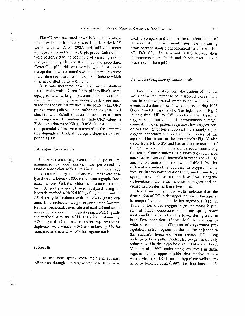
Hydrochemical data from the system of shallow wells show the response of dissolved oxygen and iron in shallow ground water to spring snow melt events and autumn base flow conditions during 1995 (Figs. 2 and 3, respectively). The light band in Fig. 2 tracing from NE to SW represents the stream at oxygen saturation values of approximately 8 mg/1. Generally, darker patterns represent low oxygen con­ditions and lighter tones represent increasingly higher oxygen concentrations in the upper meter of the aquifer. The stream in the iron panels (Fig. 3) also traces from NE to SW and has iron concentrations of 0 mg/1, or below the analytical detection limit along the reach. Concentrations of dissolved oxygen, iron and their respective differentials between annual high and low concentration are shown in Table I. Positive differentials indicate a decrease in oxygen and an increase in iron concentrations in ground water from spring snow melt to autumn base flow. Negative differentials indicate an increase in oxygen and de­crease in iron during these two times.

Data from the shallow wells indicate that the distribution of DO in the upper regions of the aquifer is temporally and spatially heterogeneous (Fig. 2, Table 1). Dissolved oxygen in ground water is pre­sent at higher concentrations during spring snow melt conditions (May) and is lower during autumn base flow conditions (September). In addition to wide spread annual infiltration of oxygenated pre­cipitation, select regions of the aquifer adjacent to the stream's hyporheic zone receive DO along recharging flow paths. Molecular oxygen is quickly reduced within the hyporheic zone (Morrice, 1997; Valett et a!., 1997) maintaining low levels in distal regions of the upper aquifer that receive stream water. Measured DO from the hyporheic wells iden­tified by Morrice eta!. (1997), i.e., locations 11, 13,

7 ~~-~J,C~1

6 15.~i:~~~f:X::.;,::;J§¥.£l;l

5 ~~~~~~~~~~~,11~.-,Jiil'ltl~'ti!ik' /''~~

4 t&£~WE~%~1i~ttS::f~---~~~.~Aim~1

3 ·\· ,··: ... ;,;~~~'Ril

1 1<''-\''r.!i'tz:'. ··c:e:::~!if~~~~

Fig. 2. Seasonal response of oxygen in ground water. The distribution of dissolved oxygen in the upper aquifer during spring infiltration (elevated oxygen) and late summer base flow conditions (low oxygen) during 1995 is represented by shades of gray.

-!=> N 0

:.. ?o 0

,<:)

~ r:; _::: t-

'-~ "" "" ·~ ....__

g "' :; ;:;· ~ Cl "' c g ._

"' ._ -.. ::0 'C ~ .... ._ v, I .... .... "'

Fe (mg/L} site wide May, 1995

z

B+

<+

H+ Sampling locations

· TR·l • Welllransed

8

7

6

5

4

3

2

1

c+

B +

H + Sampling locations

Fig. 3. Seasonal response of iron in ground water. Shades of gray represent the distribution of soluble iron in the upper aquifer during spring infiltration (low iron) and late summer base flow conditions (elevated iron) during 1995. Light tones represented low concentrations and dark tones represent elevated concentrations of iron.

:... ;., C) ..,

@, ~ iS _::::

t-

'-[ ·~ '---. g ~. ~ ~ <:l

~ -"' -""""' -~ -':£ .... -v. I .... .... '"

... N

422 A.R. Grojjinan, L.J. Crossey I Chemical Geology 161 (1999) 415-442

Table 1 Dissolved oxygen and soluble iron data from the lateral wells. Sample collection dates are from May and September, 1995

Location lD Sampling Date 1610511995 Sampling Date 191091 1995 DO Differential Fe Differential

DO (mgll) Fe (mgll) DO(mgll)

II 0.28 0.00 0.85 12 0.32 2.80 1.16 13 3.64 0.31 6.35 14 1.44 4.39 0.26 15 0.41 4.63 0.20 21 3.83 1.71 0.16 22 2.98 1.78 0.16 23 5.66 1.01 0.74 24 0.66 2.10 0.38 25 0.12 0.00 1.12 31 0.25 0.23 0.88 32 0.14 2.25 1.15 33 2.24 0.23 1.12 34 3.84 0.77 0.28 35 5.40 0.54 0.24 41 1.10 0.23 0.76 42 1.83 0.15 0.50 44 2.14 0.31 1.87 45 0.25 1.55 0.22 51 1.42 0.39 0.54 52 1.31 0.62 0.22 53 0.53 1.01 0.27 54 3.56 0.23 0.50 55 2.86 0.39 0.31 56 1.50 0.20 0.20 B 5.98 0.31 ' 0.29 c 0.49 0.54 0.24 D 1.03 0.70 1.27 E 4.87 2.88 0.76 F 4.97 0.00 0.41 G 4.95 0.70 1.36 H 2.62 2.41 2.09

6.69 0.46 5.40 0.56 0.77 1.81

K 2.70 0.23 1.19 L 2.40 6.88 0.28 M 0.87 7.29 1.57 z 3.15 0.54 1.54 Median 1.99 0.58 0.64 Minimum 0.12 0.00 0.16 Maximum 6.69 7.29 6.35

25 and 42 (Table 1 ), show elevated DO and dimin­ished iron concentrations at recharging flow paths adjacent to the stream.

The distribution of iron in shallow ground water has an inverse relationship with that of oxygen (Figs. 2 and 3; Table 1). Iron is generally low at the top of

Fe (mgll) (mgll) (mgll)

0.00 -0.57 0.00 0.68 -0.84 -2.13 0.00 -2.71 -0.31 3.68 1.18 -0.71 8.07 0.21 3.44 6.73 3.67 5.03 9.52 2.82 7.74 1.63 4.92 0.62 3.43 0.28 1.34 0.25 -1.00 0.25 0.65 -0.63 0.42 2.81 -1.01 0.56 1.54 1.12 1.31 0.76 3.56 -0.01 3.76 5.16 3.22 1.30 0.34 1.07 0.25 1.33 0.10 1.30 0.27 0.99 3.52 0.03 1.97 0.85 0.88 0.46 3.02 1.09 2.40 9.95 0.26 8.94 0.85 3.06 0.62 0.57 2.55 0.18 0.51 1.30 0.31 0.50 5.69 0.19 0.70 0.25 0.16 2.61 -0.24 1.91 0.00 4.11 -2.88 3.77 4.56 3.77 0.42 3.59 -0.27 4.46 0.53 2.05 0.00 1.29 -0.46 6.11 -1.25 5.33 0.32 1.51 0.09 9.32 2.12 2.44 8.15 -0.70 0.86 6.53 1.61 5.99 1.42 1.11 0.62 0.00 -2.71 -2.88 9.95 5.69 8.94

the water table during spring snow melt infiltration and increases markedly during autumn base flow conditions. Site wide differentials between May and September 1995 show an overall increase in iron in ground water as biogeochemically induced redox conditions shift from aerobicjsuboxic conditions

A.R. Groffinan, L.J. Crosse_v /Chemical Geology 161 (1999) 415-442 423

during spring snow melt to suboxicjanoxic condi­tions during late summer and autumn.

Shift in DO and iron concentrations .from spring to autumn is graphically displayed in Fig. 4 where data, independent of location, has been sorted, ranked and plotted according to concentration. Fig. 4 shows pronounced difference in both iron and oxygen con­centrations between spring infiltration (May) and autumn base flow conditions (September /October) throughout most of the aquifer. Select portions of the aquifer do not seem to be sensitive to seasonal changes, for example locations L and M (Figs. 2 and 3; Table I) consistently exhibit elevated iron and relatively low oxygen throughout the year and re­spond only weakly to infiltration pulses. This region

~ Cl §. 0 0

10

9 Population (n=38)

7

6

5

4

3

2

8

7

6

6

4

3

2

Fe(mg/L) Range Oto 1 lto2 2 to3 3 to 4 4to 5 >5

Number of sampling locations May September/October 24 17 5 4 5 2 0 6 2 1 2 8

Increasing Fe

Population (n=38) DO(mg!L) Range 0 to 1 1 to 2 2to3 3 to6

Number of sampling locations May September/October 12 24 7 11 7 1 12 2

Increasing DO

may be hydraulically isolated with weak exchange between surrounding environments.

3.2. Vertical redox fluctuations

Vertical profiles of redox sensitive constituents show the biogeochemical response of the aquifer to infiltration events. Data from two biogeochemically diverse locations, one periodically oxic and one con­sistently reducing are compared below (Figs. 5-8). The first location, MLS-3 (Fig. I), is situated in a relatively reduced portion of the aquifer character­ized by consistently suboxic to anoxic conditions and shows a weak response to annual infiltration events.

A. Site wide Fe distribution

B. Site wide DO distribution

Fig. 4. Comparison between soluble iron and dissolved oxygen in shallow ground water during minimum and maximum concentrations; spring infiltration/late summer base flow, 1995. Data has been sorted with respect to concentration without reference to location in the aquifer.

424 A.R. Gro.f]inan. L.J. Crossey j Chemical Geology 161 (1999) 415-442

DO (mg!L)

0 "' "' 0 "' 0 "' 0 ...

( -= !!l "' "'

8 I I 't

§ I I

8 I ,....,

! "'

03/~1971 I !!l I

'§. B c 06/~/971 ., ~

04/26/97 05/16/97 Cl

l 0 "' 0 "' "' 0 "' "' 0

....::!...._ ....::!...._ ....::!...._ -= -= -=

8

§ I

8 I

"' !!l

09/~1971 E F

~ 07/09/97 07/30/97

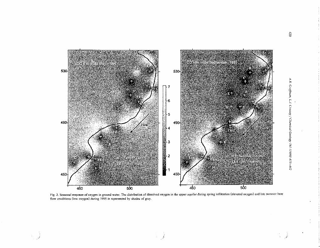
Fig. 5. Vertical profiles of dissolved oxygen in the upper aquifer at MLS-3 from March through September, 1997.

The second site, MLS-1 (Fig. 1), is located in a portion of the aquifer that experiences annual fluctu­ations in redox biogeochemistry and is sensitive to the annual infiltration cycle. Hydrochemical data used to plot Figs. 6 and 8 are shown in Table 2.

Data from vertical profiles indicate that the pa­rameters most sensitive to infiltration pulses are oxy­gen, iron and sulfate. Manganese concentrations ap­pears to be Jess responsive to changes in Eh and DO and are more persistent temporaily and spatiaily than iron. Chloride is included as a conservative con­stituent because it is not affected by redox processes. Chloride in ground water is sensitive to the effects of concentration and dilution (Ailison and Hughes, 1978; Anderholm, 1994). An increase of chloride in the upper profile suggests concentration due to evap­otransporation, transport of concentrated solute from

the overlying vadose zone, or both. Decreasing con­centrations within a vertical profile suggests dilution from infiltration or the influence of more dilute waters flowing along preferential flow paths. Iron, manganese and sulfate are nonconservative; that is, susceptible to the same processes as chloride but are also subject to precipitation, sorption and are used by bacteria in tenninal electron accepting processes (TEAPs) (Chapeile, 1993; Vroblesky and Chapeiie, 1994). Thus by comparing concentration profiles of chloride to sulfate, iron and manganese, physical processes can be separated from biogeochemical and hydrochemical processes. Of these processes, the increase of soluble iron and manganese and decrease of sulfate and oxygen concentrations in ground water with circumnutral pH are most likely due to TEAPs (Chapeiie, 1993; Lovley and Chapeiie, 1995).

A.R. Grojjinan, L.J. Crossey /Chemical Geology I 61 (/999) 415-442 425

Concentration (mg!L) 0

0 ..., ... 01 CD 0 ;; :;: 0 ..., ... 01 CD 0 ;; ; 0 ..., ... 01 CD 0 ;; ;

Fe (mgll) Fe (mgll) Fe (mgll) ...,

A. I B. I C. I D. I 0

e 2!

Mn' CD 0

8 !'l

e I § ..c § "E. "'

80

Mn (mg/L) Mn (mg/L) Mn (mg/L) Mn (mgll) Cl

0 0 N 0 0 ..., 0 0 ...,

1 0 ...,

b

'" b '" b '" '" b "' b '" b '" b '" b

0 "' "' 0 "' ... "' 0 "' ... "' 0 "' ... "' 0 Cl and 504 (mgll) Cland 504 (mg/L) Cl and 504 (mgll) Cl and 504 (mg/L)

..., 0 A.2 C.2 D.2 B.2 e

~

2! -= Cl

g 804

8 §

e § §

8 --------·-·-·---···----------···-····---· --· ·······-· ···---·-····---------03/04/97 04/21/97 07/23/97 08/29/97

Fig. 6. Seasonal variation of biogeochemical parameters through time in a moderately reducing region of the aquifer. Vertical profiles of Fe,

Mn and S04 and Cl at MLS-3 from March through late August, 1997 illustrate the variability of redox determining constituents through a

seasonal cycle.

3.3. Suboxic to anoxic region of the aquifer (MLS-3)

Fig. 5 shows dissolved oxygen concentration pro­files with depth from late winter (March) through late summer (September) for location MLS-3. Note the fluctuation of the phreatic surface from late winter low levels (panel A) to maximum levels during spring snow melt infiltration (panel C) then back to base flow low level conditions (panel G).

Our data show that although DO is relatively low at depth, concentrations fluctuate in the upper meter of the aquifer seasonally (Fig. 5). During late winter DO is below the instrument detection limit (0.4 mgjl) from the phreatic surface of the aquifer to the depth of measurement, approximately 200 em (panel A). By April spring snow melt, DO was measured at concentrations up to I mgjl in the upper I 0 em of

the aquifer (panel B) with an oxicjsuboxic region expanding to the upper 40 em of the aquifer (panel C) by the middle of May. Dissolved oxygen concen­trations in the extreme upper regions of the aquifer increase but the region of influence decreases to approximately 20 em with the approach of early summer (panels D and E) and then sharply decreases to below instrument detection limits with depth. By mid summer, DO concentrations are at or below the instrument detection limit within the entire ground water profile measured (panels F and G) suggesting suboxic /anoxic conditions throughout this region of the aquifer. In summary, the impact of DO on ground water appears to be restricted to the upper I 0-40 em of the aquifer suggesting the existence of a transient interface between shallow oxic-suboxic and deeper persistently anoxic environments in the aquifer.

426 A.R. Grojfinan, L.J. Crossey /Chemical Geology 161 (1999) 415-442

DO(mg/L) 0 - "' "' ... U1 "' 0 - "' "' ... U1 "' 0 0 - "' "' ... U1 0> 0 - "' "' ... '" "'

_L_ "f'

!9

8

§

~ B c D 11/29196 03131197 04113/97 04126/97 .-..

5 ~ '-'

t 0 - "' "' ... U1 "' 0 - "' "' A U1 "' 0 - "' "' A U1 "' 0 r-- -

l !9 _L_ _L_

-= 8 (

§

~

Ol/~7~ F G H

~ Ol/16/97 07/09197 09/0l/97

Fig. 7. Vertical profiles of dissolved oxygen in the upper aquifer at MLS-1 from November, 1996 through September, 1997.

Hydrochemical profiles from MLS-3 are shown from late winter (February /March) to late summer (AugustjSeptember) in Fig. 6 (panels A through D). During late winter maximum snow pack (panels A.1 and A.2) chloride and sulfate are below 3 mg/1 and exhibit relatively constant concentrations with depth. Iron and manganese at this time show a slightly increasing trend towards the top of the aquifer but remain below 10 and 2 mg/1, respectively. The phreatic surface at this time is approximately 50 em below land surface (BLS). With the onset of spring snow melt (April), iron and manganese concentra­tions increase markedly above 120 em, chloride re­mains constant and sulfate concentrations exhibit a 20% decrease above 120 em (B.1 and B.2, Fig. 6; Table 2). The phreatic surface at this time has risen to approximately 40 em BLS. By mid summer (late July) iron is present at relatively high concentrations

(7-10 mg/1 in the upper 120 em of the water table) and decrease with depth (5-7 mgjl) (C.l, Fig. 6; Table 2). Except for an anomalous point at 130 em, manganese fluctuates slightly about a median con­centration of 1.03 mgjl throughout the measured profile. Sulfate shows a decrease in concentration at depths above 120 em suggesting that robust sulfate reduction is occurring within this interval. This may represent a transition from a strict iron to a combined iron and sulfate dominated redox regime. Note the increase in chloride concentrations at depths above 80 em (C.2, Fig. 6; Table 6) and a decrease in the phreatic surface since April. By late summer (AugustjSeptember) sulfate concentrations have de­creased well below I mg/1 above a depth of 120 em and chloride is concentrated at the top of the water table. Iron and manganese concentrations are rela­tively high throughout the profile (6-12 mg/1 Fe

A.R. Grojjinan, L.J. Crosser I Chemical Geology 161 (/999) 415-442 427

Concentration (mg/L) --------~ a a a a a a b w in "' b b w

A.l Fe (mg/L) B.l Fe (mg/L) C.l

...1.__ Fe

Mn (mg/L)

a a "' a a b in b "' b b in a - "' "' " U1 Ol .... a - "'

B.2 Cl and S04 (mg/L)

C.2

Cl

12/10/96 03/04/97

a a in "'

Fe (mg/L) ...1.__

Mn (mg/L)

b in

"' " U1 Ol

04/21/97

b

"' b

....

a b

a b a

D.l

-D.2

9

"'

a in

"'

a in

Fe (mg/L)

Mn (mg/L)

b

"' "

a

"'

in

U1 Ol

Cl and S04 (mg/L)

08/07/97

"' b ....

Fig. 8. Seasonal variation of biogeochemical parameters through time in an oxic I suboxic region of the aquifer. Vertical profiles of Fe, Mn, S04 and Cl at MLS-1 from March through August, 1997 illustrate the variability of redox determining constiruents through a seasonal cycle.

and 1-1 .5 mg/1 Mn) and are elevated (approxi­mately 12 and 1.5 mg/1, respectively) in the upper 20 em of the aquifer due perhaps to TEAPs and concentration effects. Data from April show a similar trend in the top 20 em of the aquifer.

3.4. Oxic to moderately reducing environments

Vertical profiles of DO concentrations from MLS-1 are shown for one annual cycle in Fig. 7 (panels A through H). The phreatic surface fluctuates by as much as 60 em throughout the year from winter low levels (panel A) to maximum levels during spring snow melt infiltration (panel F) and to late summer low levels (panel H). Generally, this location has been suboxic to weakly oxic throughout the time we have monitored DO. During early winter (panel A),

DO concentrations range from 3 to above 5 mg/1 in the upper 50 em of the aquifer and are between 2 and 3 mg/1 in the lower profile. By late March (panel B) the phreatic surface has risen to within 20 em of the land surface and DO has decreased to 2-4 mg/1 in the upper 50 em and below 2 mgjl with depth. Through the month of April the phreatic surface fluctuates in response to episodic infiltration pulses at, and up gradient from, MLS-1. Also, DO concentrations are from 2 to 3 mgjl during mid April (panel C) to < I mgjl throughout the profile during late April (panel D). By early May (panel E) DO is at the instrument detection limit throughout the profile but by the middle of May rises to approx­imately 2-3.5 mgjl) at the phreatic surface and sharply decreases to 1-2 mg/1 with depth (panel F). July and September profiles are somewhat similar

428 A.R. Groffman, L.J. Crossey /Chemical Geology 161 (/999) 415-442

Table 2 Hydrochemical data through time from vertical profiles at MLS-3 (A) and MLS-1 (B). Data was used to construct Figs. 6 and 8. Codes are: not determined (n.d.), below detection limit (b.d.i.)

Depth below LS (em) Eh (mY) pH Cl (mgjl) N03. (mgjl)

(A) Location MLS-3 March 4. 1997 53 61 70 80 89 97

106 119 127 135 148 157 165 174

April 21, /997 43 51 60 70 79 87 96

109 117 125 138 147 155 164

July 23, 1997 55 64 72 83 91

100 108 122 129 138 151 159 168 176

August 29, 1997 61 69 78

234 216 212 210 214 196 194 188 191 190 191 189 183 184

140 128 131 142 131 144 146 161 192 184 170 179 182 183

130 136 144 139 146 142 143 164 175 186 169 170 174 174

276 200 185

5.58 5.82 6.02 6.27 6.33 6.50 6.61 6.69 6.65 6.63 6.61 6.54 6.53 6.70

6.94 7.01 6.93 6.96 6.98 6.95 6.94 6.89 6.84 6.84 6.89 6.89 6.88 6.89

6.64 6.66 6.65 6.63 6.67 6.71 6.77 6.79 6.80 6.82 6.82 6.80 6.88 6.80

6.54 6.50 6.51

2.23 2.04 1.86 2.04 2.22 2.24 2.20 2.12 2.26 2.30 2.29 2.29 2.42 2.38

2.39 2.73 2.33 2.68 2.42 2.71 2.43 2.60 2.63 2.55 2.49 2.42 2.38 2.30

3.59 3.29 3.29 2.43 2.34 3.04 2.38 2.32 2.15 2.59 1.92 1.93 2.00 2.98

3.47 2.61 2.70

0.61 0.42 0.37 0.31 0.18 om 0.05 0.04 0.03 0.02 0.02 O.oi 0.01 0.01

0.49 0.58 0.49 0.53 0.43 0.47 0.41 0.44 0.44 0.42 0.38 0.39 0.38 0.37

0.17 0.05 0.41 0.08 0.09 0.14 0.11 om 0.17 0.24 0.07 0.08 0.08 0.13

0.05 0.03 0.05

so4 (mg/1)

2.41 2.06 2.00 1.91 1.87 1.98 1.91 2.21 2.54 2.61 2.51 2.54 2.68 2.68

2.73 2.65 2.60 2.67 2.70 3.18 3.06 3.96 4.01 3.87 4.02 3.91 3.82 3.66

0.31 0.32 0.32 0.71 1.19 1.22 1.05 2.83 2.92 2.86 2.63 2.84 2.86 0.12

0.06 0.05 om

Fe (mgjl)

9.01 9.32 9.99 5.49 7.26 8.10 8.70 7.53 6.86 5.85 6.99 7.12 5.85 5.37

13.3 13.5 13.4 12.3 13.1 11.0 10.6 7.05 5.91 2.83 6.60 6.47 6.72 6.99

9.47 9.80

10.1 8.18 8.00 8.67 8.18 6.59 7.35 6.27 5.91 5.63 5.63 5.32

12.42 11.43 n.d.

Mn (mgjl)

1.43 1.61 1.61 1.18 1.21 1.02 1.11 0.97 0.97 0.95 0.89 1.18 0.26 0.25

1.72 1.53 1.46 1.57 1.39 1.31 1.39 0.89 0.93 0.95 0.92 0.87 0.95 1.00

1.08 1.23 1.28 0.99 0.91 0.94 1.13 0.78 1.94 0.76 0.77 0.94 1.08 1.08

1.53 1.43 n.d.

..

Table 2 (continued)

Depth below LS (em)

August 29, 1997 88 97

105 114 127 135 143 156 165 173 182

(B) Location MLS-1 December 12, 1996

72 81 89 94

102 Ill 119 132 140 149 162 170 179 187

March 4, 1997 33 41 50 60 69 77 86 99

107 115 128 137 145 154

April 21, 1997 22 30 39 49 58 66 75 88

A.R. Groj(inan, L.J. Crossey /Chemical Geology 161 (/999) 415-442

Eh (mY)

145 131 129 142 125 145 139 173 177 158 237

n.d. n.d. n.d. n.d. n.d. n.d. n.d. n.d. n.d. n.d. n.d. n.d. n.d. n.d.

292 263 267 277 278 280 284 276 281 285 287 235 286 288

355 344 352 357 378 398 410 410

pH

6.50 6.50 6.51 6.58 6.64 6.64 6.68 6.66 6.66 6.71 6.63

5.67 5.90 6.00 6.26 6.38 6.49 6.54 6.60 6.67 6.66 6.70 6.72 6.73 7.07

6.25 6.70 6.75 6.72 6.72 6.78 6.79 6.95 6.98 7.04 7.05 n.d. 7.11 7.09

6.93 7.02 6.93 6.90 7.07 7.13 7.13 7.16

Cl (mgjl)

2.76 2.30 1.88 2.18 2.25 2.02 1.55 1.89 1.80 1.80 1.80

1.50 1.42 1.40 1.42 2.74 2.58 2.86 2.38 2.31 2.43 2.32 2.84 2.82 1.53

2.68 2.37 2.04 2.01 2.07 2.09 2.12 2.07 1.89 1.91 1.90 1.93 1.98 1.95

6.02 4.48 3.84 3.09 1.99 0.14 0.14 1.89

N03 (mg/1)

0.03 0.02 0.00 o.oz 0.05 0.00 0.05 0.02 0.03 0.05 0.06

0.14 0.77 0.08 0.02 0.23 0.14 0.17 0.16 0.22 0.14 0.17 0.20 0.21 0.17

0.46 b.d.l. 0.01 O.o7 0.05 0.04 0.06 o.oz 0.14 0.15 0.14 0.15 0.16 0.16

0.46 0.42 0.43 0.38 0.73 0.75 0.83 0.85

so4 (mg/1)

0.50 0.50 0.52 2.71 4.88 2.93 2.88 2.95 2.80 2.70 2.72

3.05 3.12 2.42 2.37 3.42 3.48 3.71 3.70 3.75 3.75 3.76 3.75 3.72 1.96

2.95 3.37 3.02 3.10 3.02 2.96 3.06 2.88 3.45 3.56 3.70 3.57 3.51 3.49

4.81 4.22 4.16 4.10 4.13 4.22 4.18 4.25

Fe (mg/1)

8.51 9.15 8.83 7.22 n.d. 6.90 n.d. 6.27 6.27 6.27 6.27

3.05 2.35 0.97 1.32 7.70 1.39 0.47 0.40 0.67 0.40 0.11 0.65 2.28 1.44

b.d.l. b.d.l. b. d.!. O.o7 b.d.l. 0.07 0.04 0.75 0.04 0.04 b.d.l. b. d.!. b. d.!. 0.01

b.d.l. b. d.!. b. d.!. b. d.!. b. d.!. b.d.l. b. d.!. b.d.l.

Mn (mgjl)

0.99 1.03 1.08 0.86 n.d. 0.99 n.d. 1.18 1.18 1.03 1.03

0.78 0.97 0.49 1.26 0.55 b.d.l. b.d.l. b.d.l. 0.05 b.d.l. b.d.l. 0.05 0.50 1.00

b.d.l. 1.89 0.96 0.44 0.92 1.26 1.05 1.54 0.06 b.d.l. b.d.l. b. d.!. b. d.!. 0.06

1.08 1.22 0.93 0.78 0.09 0.05 0.06 0.06

429

430 A.R. Groffman, L.J. Crossey /Chemical Geology 161 (1999) 415-442

Table 2 (continued)

Depth below LS (em) Eh (mY) pH Cl (mgjl)

Apri/21, 1997 96 410 7.17 1.90

104 420 7.20 1.97 117 430 7.21 0.14 126 428 7.19 1.90 134 427 7.22 1.89 143 421 7.26 1.92

August 9, 1997 61 251 7.45 6.17 69 251 7.35 6.36 78 264 6.80 4.46 88 314 6.86 3.27 97 354 6.88 3.44

105 369 6.86 2.44 114 380 6.95 3.29 127 389 6.89 2.50 135 398 7.07 3.33 143 406 7.09 2.84 156 409 7.08 2.92 165 419 7.10 3.41 173 427 7.12 3.16 182 432 7.14 3.09

ranging from slightly Jess than 2-3 mg/1 with a slight decrease in concentration with depth. During this time the phreatic surface has dropped to the stable low levels of base flow conditions.

Hydrochemical data from December 1996 through August 1997 are shown from MLS-1 in Fig. 8 (panels A through D) and Table 2. December repre­sents low phreatic surface, deep base flow conditions with little if any infiltration to the subsurface. Iron and manganese concentrations range from 1-3 mg/1 and 0.8-1.3 mg/1, respectively above 100 em and generally decrease with depth (0.1-2.3 mgjl Fe and 0-1 mgjl Mn) (panel A. I). Chloride and sulfate concentrations have coincident distributions with depth. The sulfate data suggest little if any evidence for sulfate reduction (panel A.2). Data from March incipient snow melt (panels B.l and B.2) show low iron and significant manganese levels above II 0 em with concentrations for both constituents near the instrument detection limit below that depth. Vertical profiles of chloride and sulfate at this time show very little variability with depth except near the phreatic surface where chloride concentrations in­crease from approximately 2-3 mgjl in the top 20

N03 (mgjl) S04 (mgjl) Fe (mgjl) Mn (mgjl)

0.79 4.18 b.d.l. 0.06 0.78 4.29 b.d.l. 0.06 0.79 4.21 b.d.l. 0.06 0.78 4.21 b.d.l. 0.06 0.78 4.25 b.d.l. 0.03 0.81 4.22 b.d.l. 0.04

0.06 3.14 0.34 1.33 0.05 0.47 0.42 n.d. n.d. n.d. n.d. n.d. n.d. n.d. n.d. n.d. n.d.

3.59 0.37 1.33 4.45 0.51 0.20 4.09 0.42 0.15 4.32 0.42 0.10 4.14 0.40 0.17 4.29 0.34 0.16 4.13. 0.40 0.29 4.69 0.54 0.06 4.81 0.54 b. d.!. 4.80 0.56 0.04 4.82 0.56 0.01 4.81 0.54 0.02 4.80 0.54 0.04

em of the water table. Low iron, high manganese, increased chloride and a 20 em rise in the water table suggest infiltration of incipient snow melt to the upper aquifer. Towards maximum snow melt, the end of April (panels C.l and C.2), the water table rises to within 20 em of the land surface, iron is Jess than the analytical detection limit and manganese concentrations are elevated within the upper 40 em of the aquifer but decrease rapidly below this level. Chloride concentrations are high in the upper 40 em of the aquifer. Sulfate is remarkably consistent with depth except for the upper 10 em of the aquifer where it increases from 4-5 mgjl. The elevated water table and absence of iron in this time interval suggests that molecular oxygen is high enough to inhibit iron mobility but low enough to allow man­ganese to persist in ground water inferring a suboxic to oxic redox regime in the upper aquifer. Elevated chloride in the top 40 em of the aquifer suggests concentration through soil washing of residual pore fluids since evapotransporation effects due to abun­dant recharge are probably minimal during this time of year. By mid August (panels D.l and 0.2) early base flow conditions cause a lowering of the water

..

..

A.R. Groffman, L.J. CrosseyjChemica/Geology 161 (/999) 415-442 431

table by 40 em. Hydrochemical data show a slight rise in iron and manganese concentrations within the vertical profile at this time. Chloride concentrations are elevated in the upper 20 em of the aquifer suggesting some concentration through evapotrans­poration. Sulfate concentrations, however, are dimin­ished by almost 30% within this same interval.

4. Discussion

From a biogeochemical perspective, our data show that redox at Rio Calaveras is potentially controlled by molecular oxygen (H 20/H 20 2 ) in oxic and sub­oxic zones, iron (Fe3+ /Fe2+) and manganese (Mn4 + jMn2 +) in suboxicjanoxic zones and sulfur (SO}- jHS-) in anoxic regions of the aquifer. Methane distribution coincides with sulfate reduction in regions of the aquifer that are somewhat reducing (Baker, I998). These redox zones undergo temporal and spatial shifts in response to seasonal infiltration events. Instead of sharp distinctive interfaces, there is an overlap of redox zones especially in regions of the aquifer where iron and manganese exist in the presence of molecular oxygen and in zones where sulfate and iron reduction take place simultaneously. These overlapped zones are likely reactive regions of the aquifer where reaction products, i.e., solid phases of iron and manganese oxyhydroxides and sulfides, are likely to be formed and deposited on sediments forming reservoirs of their respective constituents.

4.1. Redox relationships among oxygen, iron, man­ganese and sulfur

4.1.1. Oxygen Oxygen, the primary oxidant in the system, re­

mains relatively low (less than 2 mg/1 (63 f.LM)) with maximum concentrations during spring/ early summer and minimum concentrations during late summerjautumn base flow conditions. DO concen­trations are higher in the upper regions of the aquifer and diminish with depth suggesting that oxygen is quickly reduced during transport through the vadose zone and in the upper reaches of the water table.

Oxygen coexists with ferrous iron, manganese and HS- in the upper aquifer where redox overlap occurs. At high partial pressures, oxygen oxidizes

hydrogen sulfide and ferrous iron, a kinetically fast reaction (Hem, I967; Langmuir, I997), and moder­ately oxidizes manganese, a kinetically slow reaction (Morgan, I967; Hem, I98I). When concentrations of dissolved oxygen are relatively low (suboxic or ::::;; I mg/1 (32 uM)), both biologically mediated (Tebo et a!., I997) and abiotic (Hem, I981) oxidation reac­tions decrease moderately for Fe 2 + and HS- and decrease markedly for manganese, especially at cir­cumneutral pH. This suggests that the absence of FeZ+ and HS- under aerobic conditions is a good indicator of oxygenated infiltration events in the upper aquifer. However, Mn2 +, being less reactive in the presence oxygen, persists in ground water under both suboxic and weakly oxidizing (I-2 mgjl) envi­ronments which are commonly present at the top of the phreatic surface.

4.1.2. Iron Lateral variation of ferrous iron in the upper water

table range from below the instrument detection limit (0.05 mgjl; I f.LM) to approximately I5 mg/1 (268 f.LM). When above I mg/1, iron acts as a redox buffer maintaining low levels of oxygen and selec­tively reducing manganese. This is particularly true at the top of the water table where ferric oxidation products form and are commonly observed on sedi­ments exposed in excavations less than a meter deep. Dithionite (oxide and organic bound) and hydroxyl­amine (poorly crystalline) selective iron extractions from a vertical suite of sediments cored from MLS-3 shows that both extractable iron phases are abundant throughout the region of redox overlap; up to 5 wt.% dithionite extractable Fe was measured towards the top of the water table (Sterling, I996). Maximum concentrations of extractable iron and manganese on sediments are found in the zone of intermittent satu­ration (ZIS) where ground water levels fluctuate vertically in response to seasonal infiltration (Graff­man et al., I996). Because of the iron dynamics in this zone, the ZIS is a potential reservoir for trace elements and nutrients sorbed onto iron phases that reductively dissolve and precipitate through an an­nual cycle of ferrous/ferric states.

The presence of iron oxide phases on aquifer sediments has important implications for mixed re­dox environments, especially those dominated by iron and sulfate reduction. The concomitant reduc-

432 A.R. Groffinan, L.J. Crossey /Chemical Geology 161 (1999) 415-442

tion of iron and sulfate is thermodynamically feasi­ble over a range of environmental conditions but depends upon the stability, spectrum and distribution of iron oxides and the pH of the environment (Postma et a!., 1996). In this mixed redox environment, sul­fate reduction may occur where thennodynamically stable crystalline iron oxide phases dominate and iron reduction takes place where poorly crystalline amorphous phases predominate.

4.2. Sulfate

Our data shows that sulfate concentrations in the aquifer fluctuate throughout an annual cycle. Robust sulfate reduction takes place during summer, a time characterized by a low phreatic surface and episodic rain; 46 mm of precipitation was recorded on site during the month of July, 1997. Sulfate reduction has been documented by others including Morrice ( 1997) who found a slight decrease in sulfate along flow paths in the hyporheic zone and Baker ( 1998) who measured a significant decrease in ambient sulfate concentrations in response to acetatejBr solute in­jections in the same region of the aquifer.

Reducing conditions in the region of the so1-/HS- redox boundary were identified by com­paring sulfate values from the springs with site wide sulfate concentrations. Sulfate concentrations in spring water (4-5 mgjl) represents the stable back­ground sulfate level that is introduced into the sys­tem. Sulfate concentrations below I mg/1 and HS­up to 0.6 mg/1 were measured during late summer, 1997. Mineral saturation calculations using MINTEQ (Allison eta!., 1991) indicates that iron sulfide solid phases are thermodynamically over-saturated in ground water at this time. Hydrogen sulfide readily reacts with ferrous iron (Stumm and Morgan, 1981) forming solid iron sulfide phases which accordingly keeps H 2 S(aq) concentrations low in ground water. Through this mechanism, Fe2+ buffers biogenic HS­maintaining low HS(~q) in the aquifer.

4.2.1. Measured and theoretical redox Eh in ground water at Rio Calaveras is primarily

controlled by the abundance and distribution of iron and DO. Thus, temporal and spatial Eh gradients reflects the transient nature of the redox structure in the aquifer. Our data show that ORP values mea-

sured with a Pt probe are correlated with soluble iron in ground water under suboxic conditions, opera­tionally defined as dissolved 0 2 less than 0.5 mg/1. Thus, in low oxygen environments electron exchange between the Pt surface and ferrous iron species (above 0.5 mgjl) are somewhat representative of Eh in ground water (Barcelona et a!., 1989; Langmuir, 1997).

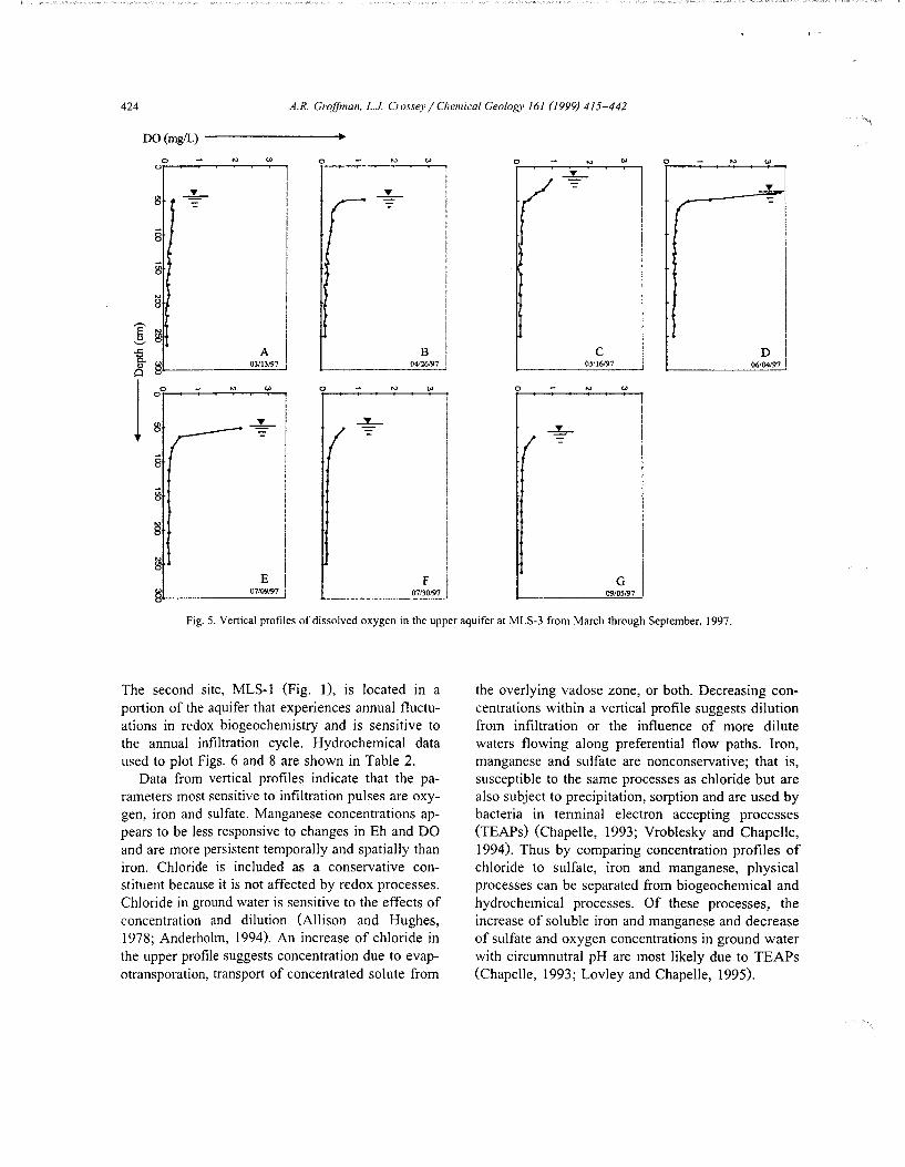
Eh and pH data from the MLS data set (Table 2) are plotted in Eh/pH space and shown in Fig. 9. Data sets has been plotted independently to illustrate general trends with depth. The arrow points from the top of the phreatic surface, in the direction of deeper ground water (1.5 m) and qualitatively represent the temporal and spatial trends in EhjpH space. Gener­ally, the data from MLS-1 shows overall higher Eh and pH, which coincides with the more oxic charac­ter of the aquifer at that location. Data from MLS-3 indicate moderately reducing conditions reflecting the suboxicjanoxic state of the aquifer. During March, late winter conditions, data from both MLS-3 and MLS-1 show steep gradients in pH and slight gradients in Eh with depth. By April (incipient snow melt) Eh gradients increase with depth with the lowest values at the ground water /vadose interface. By August the data are more scattered even though soluble iron is up to 8 mg/1 at MLS-3 and 0.5 mg/1 at MLS-1 in the upper aquifer. Eh values generally increase with depth which correlates with the distri­bution of iron, manganese, sulfate reduction and DO, i.e., higher in the upper aquifer, lower at depth. Exceptions include the MLS data sets from March and August where the August data are scattered and variable with depth and the March gradients which are so weak as to be almost insignificant.

When superimposed onto theoretical Eh-pH space (Fig. 1 0) Eh and pH data fall close to the boundary between the Fe(OH)3(solid) and Fe 2

+ stability fields. This suggests that the distribution of Fe2 + and 0 2 alternately control redox, producing ferric oxyhy­droxides in the presence of oxygen and maintaining soluble iron concentrations during anoxic conditions. EhjpH data from location MLS-1 falls within the Fe(OH)3(solid) field; ferrous iron is usually low or absent throughout the year at this location. In con­trast, data from MLS-3 consistently plot in the Fe2+ stability field just below the Fe2+ /Fe(OH)3 bound­ary. This pattern corroborates well with the hydro-

..

..

A.R. Grojjinan, L.J. Crossey /Chemical Geology 161 (/999) 415-442

~300 • -.. .z: w

250

200

. , • • • •• March 4, 1997

150 +----------r---------,----------~---------r---------,----------,----------4 6.20 6.40 6.00 6.80 7.00 7.20 7.40 7.00

pH 300 ~--------------------------------------------------------------------~

(B) 200

220

180

140

100 +--------------T--------------~------------~--------------,--------------4 5.00 5.50 6.00 6.50 7.00 7.50

pH

433

Fig. 9. Spatial and temporal trends of Eh and pH at MLS-1 (A) and MLS-3 (B). The arrows point in the direction of depth from the phreatic surface to deeper ground water along a multilevel sampling trend. Data used to construct the trend lines is shown in Table 2.

chemical data, shown in Fig. 6, where high concen­trations of soluble iron are present in ground water throughout the year. The range of values straddles

the boundary between these two phases of iron sug­gesting that precipitation and dissolution are thermo­dynamically possible in response to relatively small

434 A.R. Groffinan, L.J. Crossey /Chemical Geology 161 (1999) 415-442

400 Fe 2+ Fe(OH)3

200

.--..

:a Fe(OH)4• .._, 0 ..c

~

-200

-400

-600

-800+-------r------;-------+-------r-------r------~----~

0 2 4 6 8 10 12 14

pH

Fig. 10. Eh-pH diagram for select phases in the Fe-0-H system. Select aqueous species and solid phases are shown with measured Eh and pH data from MLS-1 and MLS-3 superimposed in EhjpH space. Diagram is after Langmuir (1997); Fe= 10- 6 M.

changes in Eh. This may be why at MLS-3 sediment bound amorphous ferric phases are more abundant in the upper 200 em of the aquifer, a reactive region

typically elevated in soluble iron throughout much of the year. Abundant ferric mineral phases on the aquifer matrix suggest that pulse infiltration may be

..

..

A.R. Gro[(man, L.J. Crossey /Chemical Geology 161 (/999) 415-442 435

Table 3 Possible redox reactions that may take place in the aquifer. Acetate is used as an electron donor to reduce various TEA. Both full and half reactions are shown

Full Reaction

(I) 202<sl + CH 3COO- + OH = 2HC03 + H20 (2) 8NO) + 5CH 3COO- + 3H+ = 4N2(gl + IOHCO) + 4H 20 (3) 8N02 + 3CH 3COO- + SH + = 4N2<gJ + 6HCO) + 4H 20 (4) Mn02<sl + CH 3COO- + 3H + = 2Mn~,~l + 2HCO) (5) 8Fe(OH)3(s) + CH 3COO- +ISH+= 8Fef,~l + 2HCO) + 20H 20 (6) so]-+ CH 3COOW= HS- + 2HCO)

a viable mechanism for the transport of oxygenated water to the phreatic surface and subsequent reaction with ferrous iron.

4.3. Electron budget approach

Because of the difficulty in measuring representa­tive redox processes and determining a system Eh in a natural environment (Bricker, 1982; Lindberg and Runnels, 1984), we have used the approach dis­cussed by Scott and Morgan (1990). Their approach evaluates the 'potential' for redox reactions by as­signing a electron reference level (ERL) to a particu­lar tier in a redox ladder at a prescribed pH (Berner, 1981). Reactions most likely to represent aquifer conditions at Rio Calaveras are shown in Table 3 with each reaction representing a redox tier. The

Table 4

Half Reaction

0 2 +4H++4e =4H 20 2NO) + 12H+ + IOe- = N2 + 6H 20 2N02 + 8H+ + 6e-= N2 + 4H 20 Mn02(s) + 4H+ + 2e- = Mn 2+ + 2H 20 Fe(OH)3 + 3H+ + e-= Fe2+ + 3H 20 SOJ- + 9H+ + 8e-= HS- + 4H 20

dominant redox reactions, species and phases that control the system, were first evaluated and the ERL chosen to act as a pem1eable boundary in Eh-pH space across which electrons flow freely; we use sulfate as a ERL in our calculations. Generally, redox-sensitive species above this level are consid­ered oxidants and thus will oxidize those species which are below the ERL. Redox species below the ERL are reductants and consequently, will reduce species positioned above the ERL. In our calcula­tions we make exceptions for aqueous Fe 2 + and Mn2 + which we identify as reductants due to their reactivity with 0 2 • We also have chosen to ignore sediment bound ferric and manganese phases focus­ing our attention to aqueous species only.

Next we calculate the electron milliequivalents (emeq) for each component in the system by multi-

Criteria for the calculation of oxidative and reductive capacity in ground water

Components (n) Valence State Numberofe- Transferred

Reducing Species DOC CH 20 C=O 4e-perC n=4 Acetate CH 3coo- C=O 4e-perC n = 2(4)= 8 Formate Hcoo- C=2+ 2e- perC n=2 Propionate CH 3CH 2C02 C1 = -2, C2 = o, C3 = o 6+4+4= 14e- n= 14 Oxalate CzOJ- C= +3 I e- perC n=2(1)=2 Iron Fef.~l Fe= +2 I e- per Fe n=l Mn Mn~a~) Mn= +2 2 e- perMn n=2

Oxidizing Species Oxygen 02(aq) 0=0 2e-per0 n = 2(2) =4 Nitrate NO) N= +5 5 e- perN n=5 Nitrite N02 N= +3 3 e- perN n=3 Manganese Oxide Mn02(s) Mn= +4 2e-perMn n=2 Ferric Oxyhydroxide Fe(OH)3<•l Fe= +3 le-perFe n=l Sulfate so]- S=6 6e-perS n=6

Table 5 Hydrochemical data and respective electron milliequivalents (emeq) values used to calculate the redox capacity budget in ground water through time at MLS-3. Data is used to construct the profiles in Fig. ll. Codes are: not determined (n.d.), below detection limit (b.d.l.)

July 03, 1997

Depth below Acetate Acetate Propionate Propionate Formate Formate Oxalate Oxalate Fe Fe Mn Mn RDC LS (em) (mgjl) (emeq, RD) (mgjl) (emeq, RD) (mgjl) (emeq, RD) (mgjl) (emeq, RD) (mgjl) (emeq, RD) (mgjl) (emeq, RD) (emeq, RD)

55 15.6 2.11 0.00 0.00 0.09 0.02 0.15 0.02 11.4 0.20 1.35 0.05 2.41 64 4.77 0.65 0.00 0.00 0.05 0.01 0.07 0.01 10.8 0.19 1.16 0.04 0.90 72 4.58 0.62 0.00 0.00 0.04 0.01 0.06 0.01 10.1 0.18 1.02 0.04 0.85 83 5.27 0.71 0.00 0.00 0.03 0.01 0.05 0.01 7.81 0.14 0.87 0.03 0.90 91 3.81 0.52 0.00 0.00 0.02 0.00 0.02 0.00 3.87 0.07 0.83 0.03 0.62

100 2.94 0.40 0.00 0.00 0.03 0.01 0.06 0.01 5.87 0.11 0.80 0.03 0.55 108 2.19 0.30 0.00 0.00 0.02 0.00 0.04 0.01 5.64 0.10 0.68 0.02 0.43 122 5.41 0.73 0.00 0.00 0.03 0.01 0.06 0.01 5.75 0.10 0.75 0.03 0.88 129 0.81 0.11 0.00 0.00 0.00 0.00 0.05 0.01 5.42 0.10 0.83 0.03 0.25

Depth below N02 N02 N03 N03 S04 S04 DO DO oxc OXC-RDC LS (em) mg/1 (emeq, OX) (mgjl) (emeq, OX) (mgjl) (emeq, OX) (mgjl) (emeq, OX) (emeq, OX) (emeq)

55 0.00 0.00 0.53 0.04 1.37 0.1 I 1.00 0.13 0.28 -2.12

64 0.00 0.00 0.25 0.02 0.96 0.08 0.60 0.08 0.17 -0.73

72 0.00 0.00 0.30 0.02 1.21 0.10 0.46 0.06 0.18 -0.67

83 0.00 0.00 0.23 0.02 2.70 0.22 0.26 0.03 0.28 -0.62

91 0.03 0.00 0.15 0.01 2.60 0.22 0.20 0.03 0.26 -0.37

100 0.00 0.00 0.18 0.01 3.91 0.33 0.20 0.03 0.37 -0.18

108 0.00 0.00 0.27 0.02 4.16 0.35 0.18 0.02 0.39 -0.04

122 0.00 0.00 0.27 0.02 4.43 0.37 0.17 0.02 0.41 -0.47

129 0.01 0.00 0.02 0.00 4.31 0.36 0.16 0.02 0.38 0.14

..,. "' 0\

:... ?o ~ ~ ~ iS ·"' t--~

~ "' "' -~

" n :::-"' :: ;:;· e.. Cl "' 0

g ..... 0, ..... --.. ~ '0 ~ .... ..... '"" I .... .... "'

July 23, 1997

Depth below Acetate Acetate Propionate Propionate Formate LS (em) (mgjl) (emeq, RD) (mgjl} (emeq, RD) (mgjl)

55 0.00 0.00 0.00 0.00 0.11 64 72 83 91

100 108 122 129 138 151 159 168 176

Depth below LS (em)

55 64 72 83 91

100 108 122 129 138 151 159 168 176

0.00 0.00 0.00 0.00 0.00 0.00 0.00 0.00 0.00 0.00 0.00 0.00 0.00

N0 2

mg/1

0.00 0.00 0.00 0.00 0.00 0.00 0.00 0.00 0.00 0.00 0.00 0.00 0.00 0.00

0.00 0.00 0.00 0.00 0.00 0.00

0.00 0.00 0.00 0.00 0.00 0.00

0.00 0.00 0.00 0.00 0.00 0.00 0.00 0.00 0.00 0.00 0.00 0.00 0.00 0.00

N0 2 N03 (emeq, OX) (mgjl)

0.00 0.17 0.00 0.05 0.00 0.41 0.00 0.08 0.00 0.09 0.00 0.14 0.00 0.11 0.00 0.07 0.00 0.17 0.00 0.24 0.00 O.Q7 0.00 0.08 0.00 0.08 0.00 0.13

0.00 0.00 0.00 0.00 0.00 0.00

0.06 0.06 0.03 0.04 0.02 0.03

0.00 0.06 0.00 0.07 0.00 0.02 0.00 0.01 0.00 0.02 0.00 0.00 0.00 0.03

N03 so4

(emeq, OX) (mgjl}

0.01 0.31 0.00 0.32 0.03 0.32 0.01 0.71 0.01 1.19 0.01 1.22 O.oJ 1.05 O.QI 2.83 0.01 2.92 0.02 2.86 0.01 2.63 0.01 2.84 0.01 2.86 0.01 0.12

Formate Oxalate Oxalate Fe Fe (emeq, RD) (mgjl) (emeq, RD) (mgjl) (emeq, RD)

0.02 0.09 0.01 9.47 0.17 0.18 0.18 0.15 0.14 0.16 0.15

0.01 0.01 0.01 0.01 0.00 0.01 0.01 0.01 0.00 0.00 0.00 0.00 0.01

so4

(emeq, OX)

0.03 O.D3 0.03 0.06 0.10 0.10 0.09 0.24 0.24 0.24 0.22 0.24 0.24 0.01

0.15 0.15 0.05 0.06 0.05 0.05 0.05 0.00 0.00 0.00 0.00 0.00 0.03

0.02 O.Q2 0.01 0.01 0.01 0.01 0.01 0.00 0.00 0.00 0.00 0.00 0.00

9.80 10.1 8.18 8.00 8.67 8.18 6.59 0.12 7.35 0.13 6.27 0.11 5.91 0.11 5.63 0.10 5.63 0.10 5.32 0.10

DO DO OXC (mgjl) (emeq, OX) (emeq, OX)

0.59 0.07 0.11 0.38 0.05 0.08 0.30 0.23 0.20 0.18 0.15 0.15 0.15 0.14 0.14 0.14 0.14 0.14

0.04 O.Q3 O.Q3 0.02 0.02 0.02 0.02 0.02 0.02 O.Q2 0.02 0.02

0.10 0.09 0.13 0.14 0.12 0.26 0.28 0.27 0.24 0.26 0.26 0.04

Mn Mn ROC (mgjl) (emeq, OX) (emeq, RD)

1.08 0.04 0.25 1.23 1.28 0.99 0.91 0.94 1.13

0.04 0.05 0.04 0.03 0.03 0.04

0.78 0.03 1.94 0.07 0.76 O.Q3 0.77 0.03 0.94 0.03 1.08 0.04 1.08 0.04

OXC-RDC (emeq)

-0.13 -0.18 -0.16 -0.10 -0.06 -0.06 -0.09

0.10 0.06 0.13 0.21 0.22 0.22

-0.01

0.25 0.26 0.20 0.19 0.20 0.20 0.16 0.21 0.14 0.14 0.14 0.14 0.15

:.. ;:., s:; § :: c _::::

r <....

Q ~ ·~ -...... Q ;;; :::: ~­==..

~ ~ ._ ~ ::::: ~ ~ .... ._ '-" I .... .... '"

.... w _,

Table 5 (continued)

August 29, 1997

Depth below Acetate Acetate Propionate Propionate Fonnate Fonnate Oxalate Oxalate Fe Fe Mn Mn ROC LS (em) (mgjl) (emeq, RD) (mgjl) (emeq, RD) (mgjl) (emeq, RD) (mgjl) (emeq, RD) (mgjl) (emeq, RD) (mgjl} (emeq, RD) (emeq, RD)

61 0.00 0.00 0.00 0.00 0.00 0.00 0.00 0.00 12.4 0.22 1.53 0.06 0.28 69 0.00 0.00 0.00 0.00 0.00 0.00 0.00 0.00 11.4 0.20 1.43 0.05 0.26 78 88 97

105 114 127 135 143 156 165 173 182

0.00 0.00 0.00 0.00 0.00 0.00 0.00 0.00 0.00 0.00 0.00 0.00

Depth below N02

LS (em) mg/1

61 0.00 69 78 88 97

105 114 127 135 143 !56 165 173 182

0.00 0.00 0.00 0.00 0.00 0.00 0.00 0.00 0.00 0.00 0.00 0.00 0.00

0.00 0.00 0.00 0.00 0.00 0.00 0.00 0.00 0.00 0.00 0.00 0.00

0.00 0.00 0.00 0.00 0.00 0.00 0.00 0.00 0.00 0.00 0.00 0.00

N02 N03 (emeq, OX) (mgjl)

0.00 0.05 0.00 0.00 0.00 0.00 0.00 0.00 0.00 0.00 0.00 0.00 0.00 0.00 0.00

O.o3 0.05 O.o3 0.02 0.00 0.02 0.05 0.00 0.05 0.02 0.03 0.05 0.06

0.00 0.00 0.00 0.00 0.00 0.00 0.00 0.00 0.00 0.00 0.00 0.00

0.13 0.00 0.00 0.00 0.00 0.20 0.00 0.06 0.00 0.00 0.00 0.00

N03 S04

(emeq, OX) (mgjl)

0.00 0.06 0.00 0.00 0.00 0.00 0.00 0.00 0.00 0.00 0.00 0.00 0.00 0.00 0.01

0.05 O.o7 0.50 0.50 0.52 2.71 4.88 2.93 2.88 2.95 2.80 2.70 2.72

0.02 0.00 0.00 0.00 0.00 0.04 0.00 0.01 0.00 0.00 0.00 0.00

0.00 0.00 0.00 0.00 0.00 0.00 0.00 0.00 0.00 0.00 0.00 0.00

0.00 0.00 0.00 0.00 0.00 0.00 0.00 0.00 0.00 0.00 0.00 0.00

n.d. 8.51 0.15 9.15 0.16 8.83 0.16 7.22 0.13 n.d. 6.90 0.12 n.d. 6.27 0.11 6.27 0.11 6.27 0.11 6.27 0.11

S04 DO DO OXC (emeq, OX) (mgjl) (emeq, OX) (emeq, OX)

0.0 I 0.48 0.06 O.o7 0.00 0.01 0.04 0.04 0.04 0.23 0.41 0.24 0.24 0.25 0.23 0.22 0.23

0.24 0.17 0.14 0.14 0.14 0.12 0.12 0.13 0.13 0.11 0.12 0.12 0.12

O.o3 0.02 0.02 0.02 0.02 0.02 0.02 0.02 0.02 0.01 0.02 O.o2 0.02

0.04 O.o3 0.06 0.06 0.06 0.24 0.43 0.26 0.26 0.26 0.25 0.24 0.25

0.99 1.03 1.08 0.86 0.99 1.18 1.18 1.03 1.03 1.03 1.03 1.03

0.04 0.04 0.04 0.03 0.04 0.04 0.04 0.04 0.04 0.04 0.04 0.04

OXC-RDC (emeq)

-0.21 -0.22 -om -0.13 -0.14 -0.13

0.08 0.34 0.09 0.21 0.11 0.25 0.24 0.25

0.06 0.19 0.20 0.19 0.17 0.08 0.17 0.05 0.15 0.15 0.15 0.15

""'" ..., 00

:,..

"" ~ ~ ~ ~ r-­'--Q ~ ~

" Q ~ ~· !?...

~ c ~ ...... 0, ...... :::c ~ ~ .... ...... ..., I .... t

. .

-2.5

A.R. Groffman, L.J. Crossey /Chemical Geology 161 (1999) 415-442

-2 -1.5 OXC-RDC

-1 -0.5 0 0.5 0+-------~------~--------r-------;--------+-------;

20

40

60

80

100

120

140

160

180

Line of OXC-RDCequilibria

Reducing potential

Oxidizing potential

200~--------------------------------------~------~

439

Fig. II. Oxidative and reductive capacity plots through time at MLS-3. Dashed line represents equilibrium between the oxidative and reductive capacity of redox sensitive aqueous species in shallow ground water.

440 A.R. Groj]inan, L.J. Crossey /Chemical Geology 161 (/999) 415-442

plying the number of electrons each ion or complex could potentially donate or receive (shown in Table 4) by the concentration in millimoles. The reductant capacity (RDC) and oxidation capacity (OXC) are individually summed and subtracted from one an­other to detennine the overall budget in ground water. A negative value indicates a potentially reduc­ing environment, a positive value indicates relatively oxidizing conditions and a value at or close to zero suggests redox equilibrium with respect to the com­ponents measured in the system.

Redox capacity budgets calculated from July to August from MLS-3 data (Table 5) are graphically shown in Fig. 11. The dotted vertical line represents equilibrium where ground water is at redox equilib­rium (zero value). All three of the profiles appear to experience a shift to relatively oxidizing conditions at the 100-120 em depth. This correlates with de­creasing Fe 2 +, Mn2

+ and rising SO}- concentra­tions at approximately the same depth (MLS-3, Fig. 6).

Vertical profiles through time are transient in nature and migrate from relatively reducing condi­tions in July towards the line of redox equilibrium by late August (base flow conditions). The shift is related to elevated concentrations of organic acids measured in the upper meter of the aquifer from July to August (Table 5). Organic acids have a relatively high reducing potential with up to eight electrons transferred from reduced carbon complexes to an e­acceptor. This is highly dependent upon the form of organic carbon, e.g., 8 e- for acetate and 2 e- for oxalate (Table 4). The observed concentrations of organic acids in the upper aquifer, especially the top 20 em, are several orders of magnitude higher than other ground water studies with advection dominated systems. For example McMahon and Chapelle (1991) reported acetate up to 40 J.LM and formate as high as 60:M in a diffusion dominated aquitard adjacent to a sandstone bed. Thurman (1985) reports a range of values between 0.2 and 15 mg/1 organic carbon in ground water; as CH 20 the range would approxi­mately be 6.6-500 J.LM. The most abundant organic acid we measured in ground water was acetate with concentrations up to 15 mgjl (260 J.LM) in dialysis cells set in the top 10 em of the aquifer. Concentra­tions decrease sharply to 0.8 mgjl (14 J.LM) within 75 em of the phreatic surface. Sediment bound or-

ganic carbon, measured as ash free dry mass C, also decreases with depth from approximately 5% at the phreatic surface to 1% at 150 em below the water table (Baker, 1998). Fennentation processes which break down sediment bound organic carbon are rela­tively slow (Middelburg, 1989) which suggests that organic acids are allochthonous, and not produced in place in the high concentrations we have detected. An alternative model is that organic carbon is trans­ported to the top of the aquifer from the vadose zone, either as organic acids derived from fermentation processes in soil pores or as more complex recalci­trant fonns of organic carbon, i.e., fulvic and humic complexes, which are broken down to organic acids in the upper aquifer. Which ever the case, the trans­port of organic carbon from the vadose reservoir represents a source of energy for heterotrophic bacte­ria that in tum modifies the redox structure through TEAPs.

5. Conclusion

Redox regimes in shallow phreatic aquifers with relatively high flow velocities may be transient in nature migrating both temporally and spatially in response to seasonal changes. Biogeochemical link­ages and fluxes between atmospheric, vadose zone and ground water reservoirs transport solute and nutrients which stimulate biogenic modification of the redox structure. Chemical fluxes from the atmo­sphere provide oxygen for biological and abiotic oxidation reactions. Biogeochemical fluxes from the vadose zone supply a source of reductive compounds (organic carbon) for microbially mediated biogeo­chemical processes that moderate and maintain the redox state in the aquifer. Seasonally controlled infil­tration of snow melt and rain are thought to transport organic carbon to the upper reaches of the aquifer where redox processes are more active than at depth. This is especially evident in the upper 100 em of the aquifer at the Rio Calaveras research site. Further research is directed at delineating small scale biogeo­chemical resolution in the upper aquifer with special attention focused on measuring organic acids and other biogeochemical redox components.

. '

. . ..

A.R. Groffman. L.J. Crossey j Chemical Geology 161 (1999) 415-442 441

Acknowledgements

We would like to acknowledge Eric Bridgford and Todd Caldwell for many hours in the field and lab, Joe Sterling for sediment extractions and cation analysis, Mike Monday for countless cation analysis and Mike Henderson, Dave Johnson, Christina Ford and Rick Ortiz for field, lab and road activities. John Husler (SSU) allowed us the use of his laboratory facilities and provided much valuable advice. With­out the contributions of these researchers this project would not have been possible. Existing instrumenta­tion installed by the hyporheic research group under the guidance of C.N. Dahm, H.M. Valett and M.C. Campana and supported by grants BSR 8616438, BSR9020561 and DEB 9420510 from the National Science Foundation was used extensively for collec­tion of water samples. DMLS samplers were gra­ciously provided by Dan Ezra of Margan M.L.S. Our research was supported by grant EAR-9630285 from the Environmental Geochemistry and Biogeochem­istry Program of the National Science Foundation awarded to L.J. Crossey and H.M. Valett.

References

Allison, G.B., Hughes, M. W., 1978. The use of environmental chloride and tritium to estimate total recharge to an uncon­fined aquifer. Australian Journal of Soil Research 16, 181-195.

Allison, J.D., Brown, D .S., N ovo-Gradac, 1991. MINTEQA2/PRODEFA2, A geochemical assessment model for environmental systems: version 3.0, users manual EPAj600j3-91/021.

Anderholm, S.K., 1994. Ground-water recharge near Santa Fe, north-central New Mexico, United States Geological Survey Water Resources Investigation Report 94-4078, 68 p.

Back, W., 1966. Hydrochemical facies and ground-water flow patterns in northern part of the Atlantic Coastal Plain. US Geological Survey Professional Paper 498-A.

Back, W., Barnes, 1., 1965. Relation of electrochemical potentials and iron content to ground water flow patterns. US Geological Survey Professional Paper 498-C, 16 pp.

Baedecker, M.J., Back, W., 1979. Hydrogeological processes and chemical reactions at a landfill. Ground Water 17 (5), 429-437.

Baker, M., 1998. Organic carbon retention and metabolism in near stream ground water, unpublished PhD dissertation. Depart­ment of Biology, University of New Mexico, Albuquerque, NM.

Barcelona, M.J., Gibb, J.P., Helfrich, J.A., Garske, E.E., 1985. Practical Guide for Ground Water Sampling. lllinois State Water Survey, ISWS Contract Report 374, 94 pp.

Barcelona, M.J., Holm, T.R., Schock, M.R., George, G.K., 1989.

Spatial and temporal gradients in aquifer oxidation-reduction conditions. Water Resources Research 25 (5), 991-1003.

Berner, R.A., 1981. A new geochemical classification for sedi­mentary environments. Journal of Sedimentary Petrology 51 (2), 359-365.

Bricker, O.P., 1982. Redox potential: It's measurement and impor­tance in water systems. In: Minear, Robert A., Keith, Lawrence H. (Eds.), Water Analysis, Vol. I. Academic Press, pp. 55-83.

Champ, D.R., Gulens, J., Jackson, R.E., 1979. Oxidation-reduc­tion sequences in ground-water flow systems. Canadian Jour­nal of Earth Sciences 16 (1}, 12-23.

Chapelle, F.H., 1993. Ground Water Microbiology and Geochem­istry. Wiley, New York, NY, 424 pp.

Chapelle, F.H., Lovley, D.R., 1990. Rates of bacterial metabolism in deep coastal plain aquifers. Applied and Environmental Microbiology 56, 1865-1874.

Goff, F., Shevenell, L., Gardener, J.N., Vuataz, F.D., Grigsby, C.O., 1988. The hydrothermal outflow plume ofVilles Caldera, New Mexico and a comparison with other outflow plumes. Journal of Geophysical Research 93,6041-6058.

Groffman, A.R., Crossey, L., Sterling, J., Baker, M., 1996. Redox cycling dynamics of iron and manganese in a shallow alluvial aquifer. Abstracts and Programs of the Geological Society of America Annual Meeting, Denver, CO, p. A-352.

Hem, J.D., !967. Equilibrium chemistry of iron in ground water. In: Faust, Samuel D., Hunter, Joseph V. (Eds.), Principles and Applications of Water Chemistry. Wiley, pp. 625-643.

Hem, J.D., !981. Rates of manganese oxidation in aqueous sys­tems. Geochim Cosmochim Acta 45, 1369-1374.

Langmuir, D., 1997. Aqueous Environmental Geochemistry. Pren­tice Hall, Upper Saddle River, NJ, 600 pp.

Lindberg, R.D., Runnels, D.D., 1984. Ground water redox reac­tions: an analysis of equilibrium state applied to Eh measure­ments and geochemical modeling. Science 225, 925-927.

Lovley, D.R., Chapelle, F.H., 1995. Deep subsurface microbial processes. Reviews of Geophysics 33, 365-381.

Middelburg, J.J., 1989. A simple rate model for organic decompo­sition in marine sediments. Geochimica Cosmochimica Acta 52, 2477-2486.

McMahon, P.B., 1990. Role of bacterial C02 production in the formation of high bicarbonate ground water in the Black Creek and Middendorf aquifers of South Carolina. Unpub­lished PhD Dissertation, the University of South Carolina, Columbia, SC.

McMahon, P.B., Chapelle, F.H., 1991. Microbial production of organic acids in aquitard sediments and it's role in aquifer geochemistry. Nature 349, 233-235.

Morgan, James J ., 1967. Chemical equilibria and kinetic proper­ties of manganese in natural waters. In: Faust, Samuel D., Hunter, Joseph V. (Eds.), Principles and Applications of Water Chemistry. Wiley, pp. 561-624.

Morrice, J.A., Valet!, H.M., Dahm, C.N., Campana, M.E., 1997. Alluvial characteristics, groundwater-surface water exchange and hydrological retention in headwater streams. Hydrological Processes II, 253-267.

Morrice, J.A., 1997. Influences of stream-aquifer interactions on nutrient cycling in headwater streams. An unpublished PhD

442 A.R. Gro.fjinan, L.J. Crosse_v j Chemical Geology 161 (1999) 415-442

Dissertation, Department of Biology, University of New Mex­ico, Albuquerque, NM, 129 pp.

Postma, Dieke, Jakobsen, R., 1996. Redox zonation: equilibrium constraints on the Fe (III)jS04-reduction interface. Geochim­ica Cosmochimica Acta 60, 3169-3175.

Scott, M.J., Morgan, J.J., 1990. Energetics and conservative prop­erties of redox systems. In: Melchoir, Daniel C., Bassett, R.L. (Eds.), Chemical Modeling of Aqueous Systems II. American Cchemical Society, Washington DC, pp. 368-378.

Sterling, J., 1996. Iron phases in aquifer sediments at Rio Calav­eras, NM, Unpublished Senior Thesis, Department of Earth and Planetary Sciences, University of New Mexico, 32 pp.

Stumm, W., Morgan, J.J., 1981. Aquatic Chemistry, 2nd edn. Wiley, New York, NY, 780 pp.

Smith, R.L., Bailey, R.A., Ross, C.S., 1970. Geologic map of the Jemez Mountains, NM, USGS Misc. Geologic Investigations, Map 1-571.

Thurman, E.M., 1985. Organic Geochemistry of Natural Waters. Martinus NijhoffjDr. W. Junk Publishers, 497 pp.

Tebo, B.M., Ghiorse, W.C., van Wassbergen, L.G., Siering, P.L., Caspi, R., 1997. Bacterially-mediated mineral formation: in­sights into manganese(II) oxidation from molecular genetic and biochemical studies. In: Banfield, J.F., Nealson, K.H. (Eds.), Geomicrobiology: Interactions Between Microbes and Minerals. Reviews in Mineralogy, Vol. 35, pp. 225-260.

Toth, J., 1963. A theoretical analysis of groundwater flow in small drainage basins. Journal of Geophysical Research 68 ( 16), 4795-4812.

Triska, F.J., Kenedy, V.C., Avanzino, R.J., Zellweger, G.W .. Bencala, K.E., 1989. Retention and transport of nutrients in a third order stream in northwestern California: hyporheic pro­cesses. Ecology 70, 1893-1903.

Valett, H.M., Morrice, J.A., Dahm, C.N., Campana, M.E., 1996. Parent lithology, surface--ground water exchange, and nitrate retention in headwater streams. Limnology and Oceanography 41 (2), 333-345.

Valet!, H.M., Dahm, C.N., Campana, M.E., Morrice, J.A., Baker, M.A., Fellows, C.S., 1997. Hydrologic influences on ground­water-surface water ecotones: heterogeneity in nutrient com­position and retention. Journal of North American Benthologi­cal Society 16 (1), 239-247.

Vroblesky, D.A., Chapelle, F.H., 1994. Temporal and spatial changes of terminal electron-accepting processes in a petrolium hydrocarbon-contaminated aquifer and the significance for contaminant biodegradation. Water Resource Research 30, 1561-1570.

Wroblicky, G.J., 1995. Numerical modeling of stream-ground­water interaction, near-stream flow paths, and hydrodynamics of two first-order stream .. aquifer systems. MS Thesis, Depart­ment of Earth and Planetary Sciences, University of New Mexico, Albuquerque, NM.

Wroblicky, G.J., Campana, M.E., Valett, H.M., Dahm, C.N., 1998. Seasonal vareation in surface-subsurface water ex­change and lateral hyporheic area of two stream-aquifer sys­tems. Water Resources Research 34 (3), 317-328.

.. .