china and international housing price growth

of 47

China and International Housing Price Growth*

Yuk Ying Chang,a† Hamish Anderson,a and Song Shia,b

This version: 28 February 2017

Abstract

We document the Chinese effects on international residential property price growth. We

show housing prices grow faster following decline in growth of China’s gross domestic

product, increases in China’s savings rate, or rise in China’s risks. These results are

consistent with the notion of Chinese investing in overseas property markets when faced

with less promising investment opportunities at home and when they have the means to

invest offshore. These effects are stronger for countries where English is the primary spoken

language, with better tertiary education quality, and that exhibit lower correlations

between local property market price growth and China’s interest rate.

Keywords: international housing prices, China, overseas opportunities, investible funds, risk,

English, education

JEL Codes: G11; R20; F21

* We acknowledge Sudipto Dasgupta for suggestions. We also thank Jie Gan, Adrian Lee, Tim Riddiough, John

Wei, and Chu Zhang for comments. We thank Massey University’s Business Impactful Research Fund for funding. a School of Economics and Finance, Massey University, New Zealand.

b Faculty of Design, Architecture and Building, University of Technology Sydney, Australia.

† Corresponding Author: Yuk Ying Chang. School of Economics and Finance, Massey University (Manawatu

Campus), Private Bag 11-222, Palmerston North 4442, New Zealand; tel. +64-6-3569099 ext. 84073; email [email protected].

mailto:[email protected]

of 47

China and International Housing Price Growth

1. Introduction

Chinese investment in overseas property markets is widely covered in the media1

and draws attention from governments (e.g. the Australian, Canadian, and Singaporean

governments have imposed restrictions on overseas property buyers). Anecdotal evidence

suggests Chinese investment is significant2 and affects other countries’ real estate markets,

economies, and societies. In 2015, the global residential real estate value of US$163 trillion,

is approximately double the world’s gross domestic product (GDP) and comprises roughly

45% of mainstream global assets (Savills 2016). Therefore, even a small Chinese impact on

other countries’ real estate could represent a very large change on global asset values.

However, no systematic study has been undertaken, particularly in a global setting,

examining the Chinese impact, which has motivated our study. In particular, we investigate

(a) whether China affects international housing markets, (b) which countries are more

strongly affected, (c) and what conditions influence the effects.

Real estate studies typically focus on a single country (e.g. Lai et al. 2010; Mian et al.

2015), while multicountry studies primarily examine country-specific factors (e.g. Hott and

Monnin 2008; Burnside et al. 2016), although general developments or global factors are

also examined (e.g. Favilukis et al. 2013). However, how one country affects the global

1 For example, The Economist (“A roaring trade,” 18 June 2016), Forbes (“The flipside of China's love for

American real estate,” 16 May 2016), The Wall Street Journal (“Chinese investors pour money Into U.S. property,” 25 May 2016), Reuters (“Why Chinese investment in overseas real estate has more than doubled,” 18 August 2016), Financial Times (“Beijing clampdown slows China spending spree on US property,” 16 May 2016), and Bloomberg (“Chinese buyers hungry for Canadian homes with inquiries up 134%,”14 April 2016). 2 According to Juwai, a leading international real estate broker specializing in Chinese investors, Chinese spent

US$52 billion on foreign property in 2015, up from US$10 billion three years ago. This amount is predicted to hit US$220 billion by 2020 (see https://list.juwai.com).

of 47

housing market or the housing markets of various countries, such as this study investigates,

is rarely examined.

Primarily based on the quarterly data of 23 countries from 1993–2015, we find the

real residential housing price indices’ growth is significantly negatively associated with the

average growth of China’s real GDP in the past four quarters. In addition, it is significantly

positively associated with contemporaneous changes in China’s savings rate (investible

funds) in the same year, after controlling for common real estate explanatory variables. On

average, an approximately 0.23% increase in international housing prices follows a 1%

decrease in China’s GDP growth and an approximately 1% increase in international housing

prices is associated with a 1% increase in China’s savings rate. Given the global value of

residential real estate (Savills 2016), a 0.23% increase represents a very large economic

impact. Further, it is economically significant because the local economy generally must

grow by 0.89% more to have the same impact on its own housing prices.3

The GDP growth of the United States, the United Kingdom, or the aggregate of

France, Germany, and the United Kingdom does not have such pervasive effects as those of

China’s GDP growth. We obtain similar results when we replace China’s GDP growth with

interest rates or consumer confidence expectations and China’s savings rate by wealth

growth. These results are consistent with the notion of the Chinese investing in overseas

property markets when China has less promising investment opportunities and they have

the means (savings and wealth) to do so.4 These significant relations still exist when recent

economic downturns are excluded or when separating the differential effect of the post-

3 In this paper, the term local refers to one of the 23 countries we examine.

4 One plausible reason for this phenomenon is that the Chinese had relatively less exposure to foreign assets in

1990s in comparison to US and UK households. Hence, they were more likely to build up foreign asset holdings over our sample period than the Americans and the British.

of 47

2007 period. The relation with China’s GDP is prevalent and relatively stronger for

residential property markets in the United States, the United Kingdom, Ireland, Australia,

the Netherlands, France, Sweden, Luxembourg, South Korea, and South Africa.

Concerning the conditions under which these relations are stronger, we obtain the

following findings. First, the relations are more pronounced when economic risk is higher in

China or when the media covers more Chinese risk/uncertainty stories. Second, the

investible funds effect is more pronounced in local property markets with a lower

correlation with China’s interest rate. Third, the relations are stronger for housing markets

located in English-speaking countries. Finally, there are more apparent Chinese effects in

countries with quality tertiary education and local country real estate prices grow faster for

China’s top destinations for tertiary student migration when China is politically riskier.

We search major policy changes for international property buyers or key rule

changes that affect ease of Chinese capital outflows, but find only a few such changes in our

sample period for exploitation as exogenous changes to the relations we study. There is very

limited time-series cross-sectional variation. Therefore, we are strongly cautious and

conservative about generalisation of the results. Nevertheless, we find that corresponding

residential housing prices grow faster following a relaxation of capital outflows for Chinese

resident from China in 2007 and a relaxation for foreigners to purchase properties in

Australia in December 2008. We also find that related housing prices grow slower following

an imposition of a capital gains tax for overseas investors buying UK residential property in

April 2015 and a restriction for foreigners to buy properties in Australia in April 2010. Since

the number of the major exogenous changes is small, these changes are estimated to be

hardly useful for further formal and robust analyses.

of 47

Our work is related to two strands of research. First, we consider the effects of

external factors on local property markets, including immigration (e.g. Saiz 2003), exchange

rates (e.g. Rodríguez and Bustillo 2010), foreign capital flows (e.g. Aizenman and Jinjarak

2009), foreign direct investment (e.g. Farrell 1997), and tourism (e.g. Rodríguez and Bustillo

2010). However, our study examines the impacts of investment opportunities and the risks

of a single country, China, on international housing markets.

Second, we follow the mainstream finance literature in examining factors affecting

Chinese overseas property investment. In the Markowitz portfolio selection model (1952),

risk, returns, and correlations5 (for diversification) are the major determinants of an optimal

portfolio. Numerous studies consider these determinants, such as risk (e.g. Yao and Zhang

(2005) examine portfolio choices with risky housing), return (e.g. Meyer and Wieand (1996)

study housing returns in an asset pricing context), and diversification (e.g. Cotter et al. (2015)

investigate whether housing risk can be diversified using US data). The literature also

suggests investors prefer politically stable environments (e.g. La Porta et al. 1997). In

addition, studies find people are inclined to invest in assets for which they have more

information and with which they are more familiar (e.g. Coval and Moskowitz 1999;

Grinblatt and Keloharju 2001; Huberman 2001; Ivkovíc and Weisbenner 2005; Massa and

Simonov 2006). Economists have also long recognized the importance of information about

products on consumer behaviour (Nelson 1970).6 In this study, we examine the above-

mentioned factors. In addition, we study whether the attractive attributes of countries

5 While people may not actually make complex calculations related to theories (i.e. portfolio theory), they act

as if they do (McEachern 2011). Markowitz (1999) argues that investment diversification was well established in practice long before his seminal work in 1952 and highlights this by quoting from Act 1, Scene 1 of the Merchant of Venice as evidence that Shakespeare was not only conversant with diversification but also intuitively understood covariance. 6 Properties are also consumption products and property buyers are therefore concerned about the

environments associated with properties as well.

of 47

matter, including quality tertiary education. Real estate studies find premiums are paid for

houses in areas with quality educational institutions such as schools (e.g. Figlio and Lucas

2004).

The remainder of this paper is organized as follows. Section 2 describes the data.

Section 3 describes the methodology and states the hypotheses. Section 4 presents and

discusses the empirical results. Section 5 concludes the paper.

2. Data

Our dependent variable is growth of housing price indices. The real seasonally

adjusted quarterly housing price indices of 23 countries and their aggregate from 1975 Q1

to 2015 Q4 are obtained from Mack and Martínez-García (2011). The 23 countries are

Australia, Belgium, Canada, Croatia, Denmark, Finland, France, Germany, Ireland, Israel, Italy,

Japan, Luxembourg, the Netherlands, New Zealand, Norway, South Africa, South Korea,

Spain, Sweden, Switzerland, the United Kingdom, and the United States. The indices are

selected to be consistent with the US Federal Housing Finance Agency’s quarterly

nationwide house price index for single-family houses (formerly called the Office of Federal

Housing Enterprise Oversight house price index). The same source also provides

corresponding real seasonally adjusted quarterly personal disposable income series.

The sources of the key variables of interest are as follows: Datastream for China’s

quarterly real GDP growth since 1992, the prime lending rate, and consumer expectation;

the World Bank for China’s savings rate and annual GDP before 1992; Crédit Suisse (2015)

for China’s total wealth and wealth per adult; the PRS Group for China’s political, economic,

and financial risk ratings; Bloomberg for the numbers of China’s risk stories and all stories;

Solt (2016) for China’s Gini coefficient; Wikipedia for the classification of English countries;

of 47

Quacquarelli Symonds Limited for the QS higher education country ranking and the United

Nations for the top five tertiary student migration destinations of China.

We obtain the raw data for the other control variables from the Economic Cycle

Research Institute, Datastream, the PRS Group, Bloomberg, and the Organisation for

Economic Co-operation and Development (OECD). We obtain international business cycle

chronologies from the Economic Cycle Research Institute. Local and world GDP,

unemployment rates, exchange rates, and consumer confidence indices are from

Datastream. We obtain the political, economic and financial risk ratings of other countries

from the PRS Group and local and global numbers of risk stories and all stories from

Bloomberg. Finally, the OECD provides country-level household debt, short-term interest

rates, rental price indices, production indices in construction, and indices of permits issued

for dwellings or residential buildings. Where necessary, we convert all series into real

seasonally adjusted quarterly series using the seasonality dummy approach. For daily or

monthly series, we use the average of all days or months in a quarter. The variable

definitions are given in the Appendix.

Table 1 shows the main variable summary statistics. Over the sample period from

1993 Q1 to 2015 Q4, China’s real GDP growth is more than 10 times higher than for both local

country and world real GDP growth. On the other hand, China’s political risk is higher than

that of the 23 other countries but comparable to the overall world political risk (where a

lower rating indicates greater risk). China’s economic risk is similar to our 23 local countries’

economic risk average, while overall world economic risk is slightly higher. China’s financial

risk is also lower than its economic risk and local and world financial risk.

of 47

Table 2 reports the correlation coefficients of the major variables. The relatively

stronger correlation coefficients are mainly associated with certain risk variables. The

world’s risk story number is relatively strongly correlated with the world financial risk rating

(0.557), China’s political and financial risk ratings (-0.647 and 0.634, respectively), and

China’s and local proportions of stories about risk (0.581 and 0.617, respectively). China’s

financial risk rating is relatively strongly correlated with its economic risk rating (0.633),

world financial risk rating (0.726), and local risk story number (0.567). Lastly, the world

financial risk rating is relatively strongly correlated with the world economic risk rating

(0.512) and the local risk story number (0.502). Nevertheless, all variance inflation factors

are well below 10. Hence, multicollinearity is not a concern.

3. Hypotheses and methodology

The home bias literature shows that investors typically hold portfolios that are

overweighted towards their home market, which suggests that the Chinese will invest

mainly in Chinese-domiciled assets. However, certain factors may encourage the Chinese to

invest offshore. In particular, in a spirit similar to the notion of ‘push’ and ‘pull’ factors in

the capital flow literature (e.g. Calvo et al. 1993, 1996; Fernandez-Arias 1996; Chuhan et al.

1998; Fratzscher 2012), when there are fewer expected growth opportunities in China, the

Chinese may seek offshore investment opportunities, including residential property. As

motivation for overseas property investments, Newell and Worzala (1995) report that

investors in a survey state ‘lack of opportunities in domestic market’ and ‘higher returns

than domestic markets’ as key factors. Therefore, we predict that the Chinese will buy more

overseas properties when expected growth opportunities in China are fewer, which would

lead to faster real housing price growth (hpg) of overseas real estate markets. We call this

of 47

the overseas opportunity hypothesis. To test this prediction, we empirically estimate the

following model:

hpgj,t = a0 + a1*China’s expected growth opportunitiest + Controlsj,t + ej,t (1)

where the subscripts j and t index the country and quarter, respectively. We expect a1 to be

negative. Lemmon and Portniaguina (2006) show that the GDP is fairly strongly associated

with consumer confidence in expected macroeconomic conditions, a major determinant of

growth opportunities. Therefore, we use the average of the real GDP growth of the past

four quarters as a proxy for expected growth opportunities. In place of real GDP growth, we

also use the interest rate and consumer expectations as alternative proxies for robustness

checks.

The controls of the baseline model include lagged real housing price growth, real

personal disposable income growth, the past real GDP growth of the local economy and the

world, and country fixed effects.7 We estimate robust standard errors based on country and

time clustering. The additional controls of an augmented model are growth of the

construction production index, of the rental index, of the unemployment rate, of the

consumer confidence index, of the exchange rate, of household debt, and of the interest

rate.8 To minimize the influence of outliers, the variables of all the regressions are

winsorized at 1% and 99%.

7 The controls are based on demand fundamentals in the housing market such as employment and income

(Wheaton and Nechayev 2008; Campbell et al. 2009). We include lagged housing price growth to control for return persistence found in the housing market (Case and Shiller 1989). Based on DiPasquale and Wheaton’s model (1992), GDP growth should be significantly correlated to housing market demand. We add the world GDP growth to control for a general globalization effect on local housing markets. 8 Adding the interest rate and rent in the model will control for housing market investment opportunities.

Shiller (2006) argues that house prices should be equal to the present value of future rents. Glaeser et al. (2005) find that new construction is a key variable in explaining why US housing prices have gone up.

of 47

We estimate the baseline model for each individual country to study the prevalence

of China’s effects. To examine whether there are similar effects for other major economies,

we replicate the individual country analysis using the real GDP growth of the United States,

of the United Kingdom, and of the aggregate of France, Germany, and the United Kingdom

in place of that of China.

Regarding our second hypothesis, economics posits that when people have more

funds, they will consume and invest more (e.g. Krugman and Wells 2015). Specifically, when

Chinese individuals have more funds to invest, some of it will flow into the property market,

including markets outside China. Hence, we predict that an increase in investible funds of

the Chinese will increase their overseas property investments, which, in turn, will increase

the housing price growth of these markets. We call this the investible funds hypothesis. To

test this hypothesis, we expand Eq. (1) to

hpgj,t = a0 + a1*China’s expected growth opportunitiest

+ a2*growth of China’s investible fundst + Controlsj,t + ej,t (2)

We consider three alternative fund measures: the savings rate, aggregate wealth,

and wealth per adult. We subsequently focus on the savings rate because we only have data

on the latter two measures since year 2000. We predict a positive a2. Since Chinese

participants in overseas property markets are likely to be in the upper-middle class or higher

because of the relatively high minimum investment outlay, the ideal proxy should capture

Meanwhile, credit market terms is used to analyse the causes of the subprime mortgage crisis (e.g. Wheaton and Nechayev 2008; Khandani et al. 2009; Glaeser et al. 2010). The exchange rate may be relevant for international investors, since changes of the exchange rate will have a material impact on foreign investment. Thus, it could have predictive power in our analysis (Chen et al. 2010). Finally, the consumer confidence index is based on the exuberance theory proposed by Akerlof and Shiller (2009), to counter for the recent bubble period.

of 47

this group’s investible funds. We therefore use the growth of the product of an existing

investible funds measure and the Gini index. Larger Gini measures imply greater income

inequality within a nation, thereby capturing the ability to accumulate savings and wealth of

those in or above the upper-middle classes.

Concerning our third hypothesis, risk is a primary consideration of any investment

(Markowitz 1952), including property. Miles (2009) reports a 1% increase in uncertainty

lowers changes in housing starts by almost 1%. However, analogous to the overseas

opportunity hypothesis, when risk in China is higher, the Chinese invest less in China and

turn to overseas investment. A safe investment has been given as a very important reason

for Chinese overseas property purchases (Gu and Talyor 2015; Rubina 2016). Consequently,

we expect an increase in risk in China will increase overseas property investments by the

Chinese, thus accelerating the growth of foreign housing prices. We call this risk hypothesis.

We thus augment Eq. (2) as follows:


+ a2*growth of China’s investible fundst + a3*China’s riskt

+ Controlsj,t + Risk Controlsj,t + Global Risk Controlt + ej,t (3)

The prediction is that a3 is positive. We have four Chinese risk measures: political,

economic, and financial risk ratings and the proportion of risk or uncertainty stories,

estimated as the ratio of the number of risk and uncertainty stories to the number of all

stories. Since the ratings are inverse risk measures, their coefficients are expected to be

negative. We simultaneously incorporate these different risk measures and use local risk

of 47

counterparts as new controls. We also include global risk controls because foreign housing

markets are integral parts of the world.

As our final hypothesis, China’s effects predicted by the three hypotheses above are

likely to vary across countries. The variation conceivably depends on how familiar the

Chinese are with the countries in question (e.g. Coval and Moskowitz 1999; Grinblatt and

Keloharju 2001; Huberman 2001; Ivkovíc and Weisbenner 2005; Massa and Simonov 2006)

and how attractive these markets are to the Chinese, including aspects such as English being

the primary language and quality tertiary education (e.g. Figlio and Lucas 2004). In other

words, familiarity and attractiveness are expected to moderate the Chinese effects on the

growth of foreign housing prices. We therefore modify Eq. (3) accordingly:


+ a2*growth of China’s investible fundst + a3*China’s riskt

+ Controlsj,t + Risk Controlsj,t + Global Risk Controlt

+ a1m*Familiarityj(,t)/Attractivenessj(,t)*China’s expected growth opportunitiest

+ a2m*Familiarityj(,t)/Attractivenessj(,t)*growth of China’s investible fundst

+ a3m*Familiarityj(,t)/Attractivenessj(,t)*China’s risk + ej,t (4)

If a familiarity/attractiveness attribute strengthens (weakens) the Chinese effects,

a1m will be negative (positive) and a2m and a3m positive (negative). The main effects of the

familiarity/attractiveness attributes are not incorporated for a more parsimonious model

because either there is no main standalone effect or the main standalone effect cannot be

estimated with country fixed effects.

of 47

The attributes we consider sequentially and cumulatively are the correlation

between China’s interest rate and the growth of overseas housing prices (reflecting

diversification benefits), primary languages, and quality of higher education. Modern

portfolio theory (Markowitz 1952) states that whether we add an asset to an existing

portfolio depends on the asset’s incremental risk effect on the portfolio. If the asset is

strongly positively (weakly) correlated with the portfolio, there is little (more) room for risk

reduction. Therefore, an investor is more likely to invest in an asset if its correlation with the

investor’s existing portfolio is lower. The return series of the Chinese portfolio is not readily

available. However, as the home bias literature suggests, the Chinese likely mainly hold

assets in China. It is thus plausible to use a series that reasonably tracks changes of the

returns of Chinese assets over time as a proxy for the return series of the Chinese portfolio.

In particular, we use the prime lending rate.9 We have two correlation measures: correlation

based on all non-contemporaneous observations and correlation for odd (even) quarters

based on even (odd) quarter observations.

Since English is a principal international language, we expect the Chinese to be more

familiar with countries where English is the primary language (English countries). We also

predict that the benefits associated with English make these countries more attractive to

the Chinese. Hence, real estate in English countries will be more appealing to the Chinese.

The Chinese effects on housing price growth will thus be stronger among these countries.

We also have two English measures: a dummy for countries where English is the primary

language (Australia, Canada, Ireland, New Zealand, the United Kingdom, and the United

9 Several Chinese interest rate series (short-, medium-, and long-term major loan rates, a discount rate, and the prime lending rate) are highly correlated, with coefficients above 0.99.

of 47

States) and a dummy for countries where English is the de facto official and primary

language (Australia, New Zealand, the United Kingdom, and the United States).

A primary reason for overseas property purchases by the Chinese is for their

children’s education and migration (e.g. Bradsher and Searcey 2015; Juwai 2016). Therefore,

we predict that the Chinese effects are more prevalent for countries with better education.

Our two measures of higher education quality are the 2016 QS higher education country-

level ranking and a dummy for the 2013 top five tertiary student migration destinations of

China. These five countries are the United States, Japan, Australia, the United Kingdom, and

South Korea.

We also look at bilateral trade, Chinese outward foreign direct investment, Chinese

migration numbers, the overseas Chinese population and Chinese outbound tourists,

geographical distance, and the long-term growth forecasts of the foreign economies.10

However, these have neither explanatory power nor moderating effects. There are three

possible explanations. First, these variables are not good proxies of the relevant

familiarity/attractiveness. Second, the data quality is poor. Third, there is no relation along

these dimensions.

4. Empirical results

4.1 Main relations

We first graphically show the relations between housing price growth in

international markets and growth in the Chinese GDP and wealth. Figure 1A plots China’s

10

The data sources are the United Nations Comtrade Database (bilateral trade), UNCTAD (foreign direct investment), the World Bank (migration), the OECD (Chinese population and long-term forecasts), www.travelchinaguide.com (tourist numbers), and www.distancecalculator.net (distance)

http://www.travelchinaguide.com/

http://www.distancecaculator.net/

of 47

GDP growth and the housing price growth of North America, Japan, and the aggregate of

the 23 countries. The series are four-quarter moving averages. It is evident that China’s GDP

growth is negatively correlated with aggregate and North American housing price growth,

but not with Japanese housing price growth. In Figure 1B, we replace China’s GDP growth in

Figure 1A by its wealth growth, where wealth is the product of the total wealth and the Gini

index. It is clear that China’s wealth growth is fairly strongly positively correlated with the

aggregate and North American housing price growth, but not with Japan’s.

The remaining graphs show strong corresponding relations for English countries and

countries with the top third of QS rankings. The English countries are Australia, Canada,

Ireland, New Zealand, the United Kingdom, and the United States. The countries with the

top QS rankings are Australia, Canada, France, Germany, the United Kingdom, and the

United States. Figures 2A and 2C show China’s GDP growth and Figures 2B and 2D display

China’s wealth growth.

4.2 Effects of China’s GDP growth

Table 3 reports the regression results of the relation between China’s rolling average

real quarterly GDP growth over the past four quarters (past GDP growth) and the housing

price growth of the other markets around the world. The coefficient of China’s past GDP

growth is significantly negative. This result is consistent with the overseas opportunity

hypothesis, that when China’s growth opportunities are poorer, the Chinese buy more

overseas properties, whereby increasing the growth of these markets’ housing prices.11

11

We regress China’s real housing price index growth on China’s contemporaneous or lagged real GDP growth.

The coefficient of the GDP growth is significantly positive. When we replace the above GDP growth by the average of the GDP growth over the past four quarters, the coefficient is still positive but weaker. These results are consistent with the view that lower GDP growth in China reflects a lack of investment opportunities in

of 47

The result is robust with respect to the inclusion of various controls, as shown in

columns (1) to (3) of Table 3. The coefficients of the controls are generally consistent with

expectations. Moreover, the negative relation also exists for an extended sample period,12

over which we convert pre-1992 China’s annual GDP growth into quarterly GDP growth and

use the average of the pre-1992 quarterly variables of all quarters in the corresponding year,

although the relation is weaker in the earlier period. In addition, the literature (e.g. Deng et

al. 2011; Dokko et al. 2011; Krishnamurthy and Vissing-Jorgensen 2011; Kapetanios et al.

2012; Wu et al. 2012; Xu and Chen 2012) suggests that relations may be different since the

recent global financial crisis. However, we find that the significantly negative relation

persists when separating the differential effect of the post-2007 period.

We perform several other robustness checks.13 First, instead of using the past four

quarters, we look at China’s GDP growth based on past the one-, two-, and 12-quarter

intervals. All alternative intervals of past GDP growth have significantly negative relations

with overseas housing price growth. The longer the past GDP growth interval, the larger the

estimated coefficients. The magnitude of the coefficient for 12-quarter GDP growth (-0.115)

is approximately double the one-quarter coefficient (-0.056). Second, in place of past

China’s GDP growth, we consider China’s consumer expectations based on the past one, two,

three, and four quarters. In all cases, the relations with foreign housing price growth are

significantly negative. Lastly, we replace China’s past GDP growth by China’s past prime

lending rate. We obtain strongly statistically significant and qualitatively the same results.

China’s domestic market, including the domestic property market, consistent with the overseas opportunity hypothesis. In addition, consistent with the investible funds hypothesis, we find that Chinese property market returns are significantly and positively correlated with our measures of wealth or investible funds with Chinese investors. 12

The start date varies across countries, depending on data availability. 13

These results are not tabulated but are available from the authors upon request.

of 47

Interestingly, the magnitude of the estimated coefficient of China’s prime lending rate (-

0.086) is very close to that of China’s GDP growth.

Table 4 summarizes the baseline results of 23 individual countries and the aggregate

of these countries. Negative effects of China’s past GDP growth on housing price growth are

observed in 82.6% of the countries. Among 52.6% of these countries, a statistically

significant relation, at 10% or stronger, exists. For the United States, the United Kingdom,

and the aggregate, the significance level is 1% or stronger. The table also shows that past US

and UK GDP growth do not have the same pervasive relations with housing price growth in

other markets that we see for China’s GDP growth. To compare with the effects of a larger

European economy, presumably with more significant influence elsewhere, we combine the

French, German, and British GDPs. We find that the combined GDP growth also does not

have comparable pervasive effects on international housing price growth.

4.3 Effects of China’s changes in saving or wealth growth

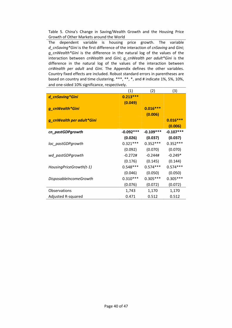
Table 5 tests and supports the investible funds hypothesis. The estimated

coefficients of all three measures of the growth of China’s investible funds are strongly

significantly positive at the 1% level.14 These results are consistent with the notion that,

when the Chinese have more investible funds, they generally increase overseas housing

purchases, thereby increasing the growth of foreign housing prices. Like the GDP growth

results, these investible funds effects are unlikely to be replicated for US wealth growth

because the correlation between the wealth growth in China and in the United States is only

14

Wealth and the savings rate without Gini interaction also have significant results. However, the saving results are stronger with Gini interaction, whereas wealth and wealth per adult have similar results whether we interact them with the Gini coefficient or not.

of 47

0.2. Meanwhile, China’s past GDP growth remains significantly negative, with a slightly

larger magnitude (changing from ─0.08 to a range from ─0.09 to ─0.11).

4.4 Effects of China’s risk

Table 6 shows the relations between the different risk measures and housing price

growth based on international panel data. In support of the risk hypothesis, the estimated

coefficient of China’s economic risk rating is significantly negative. This result suggests that,

when China’s economic risk is higher (represented by a lower rating index value), the

Chinese will invest more in foreign property markets, thereby accelerating foreign housing

price growth.15 In addition, China’s proportion of stories concerning risk or uncertainty has a

significantly positive estimated coefficient. When there are more Chinese risk stories,

therefore, the Chinese are likely to increase overseas housing investment, which, in turn,

increases the corresponding housing price growth. The other Chinese risk measures are

insignificant, except for the political risk rating, which is significantly positive when the risk

story variables are excluded.16,17

As for the local country risk measures, the coefficient of the economic risk rating is

positive and strongly significant at the 1% level, suggesting higher housing price growth

when the local economy is more stable. With regard to the world risk measures, the

financial rating has a significantly positive coefficient, whereas the proportion of risk stories

15

Since China’s and the world’s financial risk ratings are highly correlated (0.726), we drop China’s financial risk rating and rerun the regressions. The results stand. 16

China’s political risk and the world’s proportion of stories about risk/uncertainty are positively correlated. Therefore, it is possible for China’s political risk rating to be significantly positive (insignificant) when the risk story variables are excluded (included) if the world’s risk story variable subsumes China’s political risk. 17

We also separately consider changes in China’s original and relative corruption perception indices and changes in China’s corruption controls. We find no significant relationship.

of 47

has a strongly significantly negative coefficient. Hence, when the world faces lower financial

risk or appears in fewer risk stories, housing prices around the world generally grow faster.

Importantly, China’s past GDP growth is still negative and strongly significant at the

1% level. The estimated coefficient is ─0.229. Hence, on average, a 1% decrease in China’s

past GDP precedes overseas housing price increases of approximately 0.23%. This

represents an economically significant impact, given the approximate 2015 global

residential real estate value of US$163 trillion, which is double the world GDP and

represents roughly 45% of mainstream global assets (Savills 2016). Furthermore, the change

in China’s savings rate also remains significantly positive. The estimated coefficient of 0.104

indicates that a 1% increase in China’s savings rate is associated with a 0.1% increase in

international housing prices.

4.5 Modifying effects of correlation with China’s interest rate

Table 7 reveals how Chinese effects vary with the correlation between China’s

interest rate and local housing price growth. The interaction between the correlation and

changes in China’s savings rate is significantly negative. Consistent with modern portfolio

theory, Chinese investible funds effects are thus generally stronger when the correlation is

lower.18 However, the interaction between the correlation and China’s economic risk rating

is also significantly negative. This finding suggests housing prices grow faster when China

experiences better economic stability and the correlation between China’s interest rate and

local housing price growth is lower. This can be understood as follows. When China is more

economically stable, Chinese people will have stronger incentive to invest at home. Hence,

18

The effect of the growth of China’s investible funds becomes the coefficient of investible fund growth itself plus the coefficient of the interaction with the correlation and the investible fund growth.

of 47

during these times, only those foreign housing markets with higher diversification benefits

will attract more Chinese purchases in relation to those markets with lower diversification

benefits. The remaining correlation interactions are not robustly significant.

4.6 Differential Chinese effects for English countries

The second attribute we consider is the English language. As shown in Table 8,

consistent with expectations, we find that the dummies for English countries interacted with

China’s past GDP growth and with the change in China’s savings rate are significantly

stronger and have the same signs as these Chinese variables before. These results

correspondingly show more pronounced Chinese GDP growth and investible funds effects

for English than for non-English countries. There is no significant incremental Chinese risk

effect on the housing price growth of English over non-English countries.

4.7 Education matters

Table 9 reports the moderation of the Chinese effects by the education quality in the

overseas market. The interaction between education and China’s political risk rating is

negative. This finding suggests that, when China is more politically unstable, the overseas

housing markets of countries with higher-quality education are more attractive to the

Chinese, who then probably purchase more in these markets and housing prices grow faster.

Hence, education magnifies China’s political risk effects on housing price growth. On the

other hand, the interaction between education and China’s economic risk rating is

significantly positive. Hence, education strengthens the Chinese effects on overseas housing

price growth when China is more economically stable, thereby enabling the Chinese buyers

to generate more funds. The remaining educational interaction terms are insignificant at the

standard levels.

of 47

Plausibly, English countries and countries with better education also have non-

English language and non-educational characteristics attractive to Chinese buyers. One

obvious candidate is those attributes associated with the level of economic development.

Therefore, we examine whether measures of economic development replicate the English

language and education results. In particular, we look at two such measures: a dummy for

the G7 and the real GDP per capita. We find that the results do not reproduce the English

and education results. Hence, the latter are unlikely to be driven by attributes associated

with developed economies.

5. Conclusions

Using mainly the data of 23 countries from 1993 to 2015, we document the Chinese

effects on the price growth of residential real estate markets around the world. On average,

an approximately 0.23% increase in housing prices follows a 1% decrease in China’s GDP

growth or a 2.3% increase in China’s savings rate. These results are consistent with the

notion of an increase in Chinese overseas property purchases following the deterioration of

China’s growth opportunities or an increase in Chinese’s investible funds. These Chinese

effects are stronger for English countries. Property markets that have a lower correlation

with China’s interest rate also exhibit more pronounced investible funds effects.

When China’s economic risk is higher or China has more risk/uncertainty stories,

foreign housing prices also grow faster. This result suggests that higher risk in China drives

the Chinese to invest more in overseas housing markets, thereby accelerating corresponding

price growth. In addition, when China is more economically stable, real estate prices grow

faster for countries with two conditions, better education and lower correlation between

of 47

their housing markets and the China’s interest rate. Finally, when China is politically riskier,

real estate prices grow faster for China's top tertiary student migration destinations.

of 47

References

Aizenman, J., Jinjarak, Y., 2009, Current account patterns and national real estate markets, Journal of Urban Economics, 66, 75–89.

Akerlof, G.A., Shiller, R.J., 2009, Animal Spirits: How Human Psychology Drives the Economy, and Why It Matters for Global Capitalism, Princeton University Press.

Bradsher, K., Searcey, D., 2015, Chinese cash floods U.S. real estate market, The New York Times, 28 November, retrieved on 11 November 2016 from http://www.nytimes.com/2015/11/29/business/international/chinese-cash-floods-us-real-estate-market.html?_r=0.

Burnside, C., Eichenbaum, M., Rebelo, S., 2016, Understanding booms and busts in housing markets, Journal of Political Economy, 124(4), 1088–1147.

Calvo, G.A., Leiderman, L., Reinhart, C. M., 1993, Capital inflows and real exchange rate appreciation in Latin America, IMF Staff Papers, 40 (1), 108–151.

Calvo, G.A., Leiderman, L., Reinhart, C.M., 1996, Inflows of capital to developing countries in the 1990s, Journal of Economic Perspectives, 10 (Spring), 123–139.

Campbell, S.D., Davis, M.A., Gallin, J., Martin, R.F., 2009, What moves housing markets: A variance decomposition of the rent–price ratio, Journal of Urban Economics, 66, 90–102.

Case, K.E., Shiller, R.J., 1989, The efficiency of the market for single-family homes, American Economic Review, 79 (1), 125–137.

Chen, Y., Rogoff, K., Rossi, B., 2010, Can exchange rates forecast commodity prices, Quarterly Journal of Economics, 125(3), 1145–1194.

Chuhan, P., Claessens, S., Mamingi, N., 1998, Equity and bond flows to Latin America and Asia: The role of global and country factors, Journal of Development Economics, 55 (April), 439–63.

Cotter, J., Gabriel, S., Roll, R., 2015, Can housing risk be diversified? A cautionary tale from the housing boom and bust, Review of Financial Studies, 28(3), 913–936.

Coval, J., Moskowitz, T., 1999, Home bias at home: Local equity preference in domestic portfolios, Journal of Finance, 54, 1697–1704.

Crédit Suisse, 2015, Global Wealth Databook 2015, op. cit..

Deng, Y., Morck, R., Wu, J., Yeung, B., 2011, Monetary and fiscal stimuli, ownership structure, and China’s housing market, NBER Working Paper 16871.

DiPasquale, D., Wheaton, W.C., 1992, The markets for real estate assets and space: A conceptual framework, Journal of the American Real Estate and Urban

of 47

Economics Association, 20(1), 181–197.

Dmitrieva, K., 2016, Chinese buyers hungry for Canadian homes with inquiries up 134%, Bloomberg, 14 April, retrieved on 16 September 2016 from http://www.bloomberg.com/news/articles/2016-04-13/chinese-buyers-hungry-for-canadian-homes-with-inquiries-up-134.

Dokko, J., Doyle, B.M., Kiley, M.T., Kim, J., Sherlund, S., Sim, J., Heuvel, S.V.D., 2011, Monetary policy and the global housing bubble, Economic Policy, 26(66), 233–283.

Farrell, R., 1997, Japanese foreign direct investment in real estate 1985–1994, Pacific Economic Papers, No. 272, Australia – Japan Research Centre.

Favilukis, J., Kohn, D., Ludvigson, S.C., Nieuwerburgh, S.V., 2013, International capital flows and house prices: Theory and evidence, in Housing and the Financial Crisis, edited by Glaeser, E.L. and Sinai, T., University of Chicago Press, pp. 235–299.

Fernandez-Arias, E., 1996, The new wave of private capital inflows: Push or pull? Journal of Development Economics, 48 (March), 389–418.

Figlio, D.N., Lucas, M.E., 2004, What’s in a grade? School report cards and the housing market, American Economic Review, 94(3), 591–604.

Fratzscher, M., 2012, Capital flows, push versus pull factors and the global financial crisis, Journal of International Economics, 88(2), 341–356.

Glaeser, E.L., Gyourko, J., Saks, R.E., 2005, Urban growth and housing supply, Journal of Economic Geography, 6(1), 71–89.

Glaeser, E., Gottlieb, J., Gyourko, J., 2010, Can cheap credit explain the housing boom? NBER Working Paper No. 16230.

Grant, P., 2016, Chinese investors pour money Into U.S. property, The Wall Street Journal, 25 May, retrieved on 16 September 2016 from http://www.wsj.com/articles/chinese-investors-pour-money-into-u-s-property-1464110682.

Grinblatt, M., Keloharju, M., 2001, How distance, language and culture influence stockholdings and trades, Journal of Finance, 56, 1053–1073.

Gu, W., Talyor R., 2015, Market turmoil seen spurring China property purchases overseas, The Wall Street Journal, 27 August, retrieved on 11 November 2016 from http://www.wsj.com/articles/australia-worried-about-rise-in-chinese-property-buying-1440654099.

Hott, C., Monnin, P., 2008, Fundamental real estate prices: An empirical estimation with international data, Journal of Real Estate Finance and Economics, 36, 427–

of 47

450.

Huberman, G., 2001, Familiarity breeds investment, Review of Financial Studies, 14, 659–680.

Ivkovíc, Z., Weisbenner, S., 2005, Local does as local is: Information content of the geography of individual investors’ common stock investment, Journal of Finance, 60(1), 267–306.

Juwai, 2016, 6 reasons why education underpins Chinese overseas property investment, 5 July, retrieved on 11 November 2016 from https://list.juwai.com/news/2016/07/6-reasons-why-education-underpins-chinese-overseas-property-investment.

Kapetanios, G., Mumtaz, H., Stevens, I., Theodoridis, K., 2012, Assessing the economy-wide effects of quantitative easing, Economic Journal, 122, 316–347.

Khandani, A., Lo, A.W., Merton, R.C., 2009, Systemic risk and the refinancing ratchet effect, NBER Working Paper No. 15362.

Krishnamurthy, A., Vissing-Jorgensen, A., 2011, The effects of quantitative easing on interest rates: channels and implications for policy, NBER Working Paper No. 17555.

Krugman, P., Wells, R., 2009, Macroeconomics, Worth Publishers.

La Porta, R., Lopez-De-Silanes, F., Shleifer, A., Vishny, R.W., 1997, Legal determinants of external finance, Journal of Finance, 52(3), 1131–1150.

Lai, R.N., van Order, R.A., 2010, Momentum and house price growth in the United States: Anatomy of a bubble, Real Estate Economics, 38(4), 753–773.

Lemmon, M., Portniaguina, E., 2006, Consumer confidence and asset prices: Some empirical evidence, Review of Financial Studies, 19(4), 1499–1529.

Mack, A., Martínez-García, E., 2011, A cross-country quarterly database of real house prices: A methodological note, Globalization and Monetary Policy Institute Working Paper No. 99.

Markowitz, H., 1952, Portfolio selection, Journal of Finance, 7(1), 77–91.

Markowitz, H., 1999, The early history of portfolio theory: 1600–1960, Financial

Analysts Journal, 55(4), 5–16.

Massa, M., Simonov, A., 2006, Hedging, familiarity, and portfolio choice, Review of Financial Studies, 19, 633–685.

McEachern, W.A., 2011, Economics: A contemporary introduction. Cengage Learning.

of 47

Meyer, R., Wieand, K., 1996, Risk and return to housing, tenure choice and the value of housing in an asset pricing context, Real Estate Economics, 24(1), 113–131.

Mian, A., Sufi, A., Trebbi, F., 2015, Foreclosures, house prices, and the real economy, Journal of Finance, 70(6), 2587–2634.

Miles, W., 2009, Irreversibility, uncertainty and housing investment, Journal of Real Estate Finance and Economics, 38(2), 173–182.

Nelson, P., 1970, Information and consumer behaviour, Journal of Political Economy, 78(2), 311–329.

Newell, G., Worzala, E., 1995, The role of international property in investment portfolios. Journal of Property Finance, 6(1), 55–63.

NZ Herald, 2016, Chinese buyers coming back to Auckland property market, 6 March, retrieved on 16 September 2016 from http://www.nzherald.co.nz /business/news/article.cfm?c_id=3&objectid=11600974.

Rapoza, K., 2016, The flipside of China's love for American real estate, Forbes, 16 May, retrieved on 16 September 2016 from http://www.forbes.com/sites /kenrapoza/2016/05/16/the-flipside-of-chinas-love-for-american-real-estate/#4bec60c240e8.

Reuters, 2016, Why Chinese investment in overseas real estate has more than doubled, 18 August, retrieved on 16 September 2016 from http://fortune.com/ 2016/08/18/china-overseas-property-investment/.

Rodríguez, C., Bustillo, R., 2010, Modelling foreign real estate investment: The Spanish case, Journal of Real Estate Finance and Economics, 41, 354–367.

Rubina Real Estate, 2016, Chinese International Property Investment Trends in 2016, retrieved on 11 November 2016 from http://www.rubinarealestate.com/en/china/ china-2016-international-property-investment-overview/.

Saiz, A., 2003, Room in the kitchen for the melting pot: Immigration and rental prices, Review of Economics and Statistics, 85(3), 502–521.

Savills, 2016, World real estate accounts for 60% of all mainstream assets, 25 January, retrieved on 18 September 2016 from http://www.savills.co.uk/ _news/article/72418/198559-0/1/2016/world-real-estate-accounts-for-60--of-all-mainstream-assets.

Shiller, R.J., 2006, Long-term perspective on the current boom in home prices, The Economist's Voice 3.

Solt, F., 2016, The standardized world income inequality database, Social Science

http://www.nzherald.co.nz/business/news/article.cfm?c_id=3&objectid=11600974

http://www.nzherald.co.nz/business/news/article.cfm?c_id=3&objectid=11600974

http://www.forbes.com/sites/kenrapoza/2016/05/16/the-flipside-of-chinas-love-for-american-real-estate/#4bec60c240e8



http://fortune.com/2016/08/18/china-overseas-property-investment/

http://fortune.com/2016/08/18/china-overseas-property-investment/

of 47

quarterly, 97(5), 1267–1281.

The Economist, 2016, A roaring trade, 18 June, retrieved on 1 December 2016 from http://www.economist.com/news/united-states/21700660-chinese-tiger-mums-

start-college-town-housing-boom-roaring-trade.

Wheaton, W.C., Nechayev, G., 2008, The 1998–2005 housing "bubble" and the current "correction": What's different this time? Journal of Real Estate Research, 30, 1–26.

Wu, J., Gyourko, J., Deng, Y., 2012, Evaluating conditions in major Chinese housing

markets, Regional Science and Urban Economics, 42, 531–543.

Xu, X.E., Chen, T., 2012, The effect of monetary policy on real estate price growth in China, Pacific-Basin Finance Journal, 20, 62–77.

Yang, Y., 2016, Beijing clampdown slows China spending spree on US property, Financial Times, 16 May, retrieved on 16 September 2016 from https://www.ft.com/content/e1c2aa44-1b37-11e6-8fa5-44094f6d9c46.

Yao, R., Zhang, H.H., 2005, Optimal consumption and portfolio choices with risky housing and borrowing constraints, Review of Financial Studies, 18(1), 197–239.

https://www.ft.com/content/e1c2aa44-1b37-11e6-8fa5-44094f6d9c46

of 47

Appendix: Variables – Definition, Frequency, Calculations, and Exceptions

Variable Definition

C Takes a value of 1 for observations since 2008 Q1, 0 otherwise

ccg Growth in the seasonally adjusted consumer confidence indicator

cn_EconomicRiskRating Economic risk rating of China's economy; a larger value represents lower risk

cn_FinancialRiskRating Financial risk rating of China's economy; a larger value represents lower risk

cn_pastGDPgrowth after 1992 Average of quarterly growth in China's real GDP over the past 4 quarters

cn_pastGDPgrowth before or in 1992 Quarterly growth from annual growth in China's real GDP

cn_PoliticalRiskRating Political risk rating of China's economy; a larger value represents lower risk

cn_RiskStoryNum/TotalStoryNum Ratio of the number of risk stories to the number of all stories for China

cnSaving China's gross domestic savings, calculated as GDP less final consumption expenditure (total consumption), % of GDP.

cnWealth China's total wealth, in US dollars

cnWealth per adult China's wealth per adult, in US dollars

constrg Growth in the seasonally adjusted index of production in construction

corr (measure 1) Correlation between China's interest rate (prime lending rate, cnint) and the growth of the housing price of the local property market (hpg)

corr (measure 2) Correlation between China's interest rate (prime lending rate, cnint) and the growth of the housing price of the local property market (hpg)

d_cnSaving*Gini Change in China's savings rate

debtg

Growth in annual household debt. Household debt is defined as all liabilities that require payment or payments of interest or principal by a household to a creditor at a date or dates in the future. Consequently, all debt instruments are liabilities, but some liabilities – such as shares, equity, and financial derivatives – are not considered debt. According to the 1993 System of National Accounts, debt is thus obtained as the sum of the following liability categories, whenever available/applicable in the financial balance sheet of households and non-profit institutions serving the household sector: currency and deposits; securities other than shares, except financial derivatives; loans; insurance technical reserves; and other accounts payable. For households, liabilities predominantly consist of loans, particularly mortgage loans for the purchase of houses. This indicator is measured as a percentage of net disposable income.

of 47

Variable Definition

DisposableIncomeGrowth Growth in real personal disposable income

DisposableIncomeGrowth(t-1) DisposableIncomeGrowth of the previous quarter

Edu (measure 1) Country-level ranking of the 2016 QS world university ranking

Edu (measure 2) Takes a value of 1 for the top five tertiary student destinations of China in 2013, 0 otherwise

Eng (measure 1) Takes a value of 1 where English is the primary language, 0 otherwise

Eng (measure 2) Takes a value of 1 where English is the de facto official and primary language, 0 otherwise

exg Growth in the exchange rate

g_cnWealth*Gini Growth in China's wealth

g_cnWealth per adult*Gini Growth in China's wealth per adult

Gini China's Gini coefficient

HousingPriceGrowth (hpg) Growth in the real housing price index

HousingPriceGrowth(t-1) hpg of the previous quarter

interestg

Growth in the short-term interest rate. Short-term interest rates are the rates at which short-term borrowings are implemented between financial institutions or the rate at which short-term government paper is issued or traded in the market. Short-term interest rates are generally averages of daily rates, measured as a percentage. Short-term interest rates are based on three-month money market rates where available. Typical standardized terms are money market rate and Treasury bill rate.

loc_EconomicRiskRating Economic risk rating of the local economy; a larger value represents lower risk

loc_FinancialRiskRating Financial risk rating of the local economy; a larger value represents lower risk

loc_pastGDPgrowth Average of the quarterly growth in the real GDP of the local economy over the past 4 quarters

loc_PoliticalRiskRating Political risk rating of the local economy; a larger value represents lower risk

loc_RiskStoryNum/TotalStoryNum The ratio of the number of risk stories to the number of all stories for the country

permitg Growth in seasonally adjusted permits index issued for dwellings/residential buildings.

rentg Growth in the seasonally adjusted rental price index

urateg Growth in the seasonally adjusted unemployment rate

wd_EconomicRiskRating Average economic risk rating of all countries; a larger value represents lower risk

wd_FinancialRiskRating Average financial risk rating of all countries; a larger value represents lower risk

wd_pastGDPgrowth Average of the quarterly growth in the real world GDP over the past 4 quarters

of 47

Variable Definition

wd_PoliticalRiskRating Average political risk rating of all countries; a larger value represents lower risk

wd_RiskStoryNum/TotalStoryNum Ratio of the number of risk stories to the number of all stories for the world

of 47

Variable Frequency Calculation

C Monthly

ccg Monthly First calculate the monthly average in a quarter; then calculate the growth of the monthly average as the quarterly growth by taking the difference in the natural log of the values of two consecutive quarters

cn_EconomicRiskRating Monthly Average of the monthly ratings in a quarter

cn_FinancialRiskRating Monthly Average of the monthly ratings in a quarter

cn_pastGDPgrowth after 1992 Quarterly

cn_pastGDPgrowth before or in 1992 Annual Quarterly growth = (1 + annual growth)0.25 - 1

cn_PoliticalRiskRating Monthly Average of the monthly ratings in a quarter

cn_RiskStoryNum/TotalStoryNum Daily Average of the daily ratio in a quarter

cnSaving Annual

cnWealth Annual

cnWealth per adult Annual

constrg Quarterly Difference in the natural log of the values of two consecutive quarters

corr (measure 1) Quarterly For quarter t, the correlation calculation is based on all data, but excluding quarter t’s data point

corr (measure 2) Quarterly For odd [even] quarters, the correlation calculation is based on all even [odd] quarters

d_cnSaving*Gini Annual The first difference of the interaction of cnSaving and Gini, divided by 10,000

debtg Annual Difference in the natural log of the values of two consecutive years

DisposableIncomeGrowth Quarterly Difference in the natural log of the values of two consecutive quarters

DisposableIncomeGrowth(t-1) Quarterly

Edu (measure 1) 2016

Edu (measure 2) One data point

Eng (measure 1) One data point

Eng (measure 2) One data point

exg Monthly First calculate the monthly average in a quarter; then calculate the growth of the monthly average as the quarterly growth by taking the difference in the natural log of the values of two consecutive quarters

of 47

Variable Frequency Calculation

g_cnWealth*Gini Annual Difference in the natural log of the values of the interaction between cnWealth and Gini of two consecutive years

g_cnWealth per adult*Gini Annual Difference in the natural log of the values of the interaction between cnWealth per adult and Gini of two consecutive years

Gini Annual

HousingPriceGrowth (hpg) Quarterly Difference in the natural log of the values of two consecutive quarters

HousingPriceGrowth(t-1) Quarterly

interestg Monthly First calculate the monthly average in a quarter; then calculate the growth of the monthly average as the quarterly growth by taking the difference in the natural log of the values of two consecutive quarters

loc_EconomicRiskRating Monthly Average of the monthly ratings in a quarter

loc_FinancialRiskRating Monthly Average of the monthly ratings in a quarter

loc_pastGDPgrowth Quarterly Quarterly growth is the difference in the natural log of the values of two consecutive quarters

loc_PoliticalRiskRating Monthly Average of the monthly ratings in a quarter

loc_RiskStoryNum/TotalStoryNum Daily Average of the daily ratio in a quarter

permitg Quarterly Difference in the natural log of the values of two consecutive quarters

rentg Quarterly Difference in the natural log of the values of two consecutive quarters

urateg Monthly First calculate the monthly average in a quarter; then calculate the growth of the monthly average as the quarterly growth by taking the difference in the natural log of the values of two consecutive quarters

wd_EconomicRiskRating Monthly First calculate the average rating of all countries in a month; then calculate the average of the monthly ratings in a quarter

wd_FinancialRiskRating Monthly First calculate the average rating of all countries in a month; then calculate the average of the monthly ratings in a quarter

wd_pastGDPgrowth Quarterly Quarterly growth is the difference in the natural log of the values of two consecutive quarters

wd_PoliticalRiskRating Monthly First calculate the average rating of all countries in a month; then calculate the average of the monthly ratings in a quarter

wd_RiskStoryNum/TotalStoryNum Daily Average of the daily ratio in a quarter

of 47

Variable Exceptions

ccg Norway: quarterly

constrg Croatia's Source: Datastream

debtg Croatia, Israel, Luxembourg, New Zealand, and South Africa do not have data

Edu (measure 1) Croatia and Luxembourg do not have data

interestg Japan, interbank rate (source Datastream); Croatia, credit rate before or in 2004 and T-bill rate after 2004 (source Datastream)

permitg Japan and the US, monthly (source Datastream); Croatia and Italy, quarterly (source Datastream)

rentg Croatia: monthly (source Datastream)

urateg Quarterly: France, Israel, Italy, Luxembourg, the Netherlands, New Zealand, Norway, South Africa, Sweden

of 47

Table 1. Summary Statistics

The definitions of the variables are given in the Appendix.

Variable Mean Standard Deviation

25% 50% 75%

HousingPriceGrowth 0.54% 1.86% -0.56% 0.50% 1.64%

DisposableIncomeGrowth 0.35% 0.85% -0.09% 0.37% 0.84%

d_cnSaving*Gini 0.54% 0.83% -0.02% 0.40% 1.03%

g_cnWealth*Gini 13.06% 12.77% 8.32% 11.40% 23.12%

g_cnWealth per adult*Gini 11.57% 12.76% 6.84% 9.85% 21.42%

cn_pastGDPgrowth 10.14% 2.03% 8.38% 9.95% 11.28%

loc_pastGDPgrowth 0.58% 0.70% 0.26% 0.64% 0.97%

wd_pastGDPgrowth 0.71% 0.35% 0.60% 0.75% 0.95%

loc_PoliticalRiskRating 82 7 79 84 88

loc_FinancialRiskRating 40 5 37 40 44

loc_EconomicRiskRating 40 4 38 41 43

cn_PoliticalRiskRating 66 4 62 67 69

cn_FinancialRiskRating 45 3 45 46 48

cn_EconomicRiskRating 39 2 39 40 41

wd_PoliticalRiskRating 66 2 65 67 68

wd_FinancialRiskRating 37 2 35 37 38

wd_EconomicRiskRating 35 1 34 35 36

loc_RiskStoryNum/TotalStoryNum 12.15% 5.53% 7.78% 11.50% 15.31%

cn_RiskStoryNum/TotalStoryNum 11.84% 4.67% 9.11% 10.62% 14.91%

wd_RiskStoryNum/TotalStoryNum 14.59% 4.44% 10.84% 15.11% 17.16%

corr (measure 1) -0.18 0.25 -0.38 -0.24 0.02

of 47

Table 2. Correlations

The definitions of the variables are given in the Appendix. Here, hpg is HousingPriceGrowth. The bold figures are significant at 5% or stronger.

hpg (t-1)

(1) (2) (3) (4) (5) (6) (7) (8) (9) (10) (11) (12) (13) (14) (15) (16) (17) (18) (19) (20) (21)

DisposableIncomeGrowth (1) 0.156

d_cnSaving*Gini (2) 0.107 -0.030

g_cnWealth*Gini (3) 0.241 0.088 0.336

g_cnWealth per adult*Gini (4) 0.241 0.087 0.339 1.000

cn_pastGDPgrowth (5) -0.115 -0.017 0.006 -0.175 -0.187

loc_pastGDPgrowth (6) 0.155 0.071 -0.275 -0.172 -0.172 0.268

wd_pastGDPgrowth(7) 0.294 0.224 -0.137 -0.028 -0.029 0.197 0.579

loc_PoliticalRiskRating (8) 0.207 0.079 0.089 0.067 0.066 -0.074 0.040 0.010

loc_FinancialRiskRating (9) 0.004 0.054 -0.012 0.017 0.016 0.299 0.032 0.064 0.103

loc_EconomicRiskRating (10) 0.291 0.166 0.084 0.016 0.014 0.102 0.323 0.353 0.520 0.367

cn_PoliticalRiskRating (11) 0.091 0.021 0.191 0.128 0.117 0.560 0.047 0.062 0.051 0.286 0.131

cn_FinancialRiskRating (12) -0.013 -0.053 0.085 -0.180 -0.184 -0.250 -0.079 -0.215 0.012 -0.467 -0.080 -0.359

cn_EconomicRiskRating (13) -0.017 -0.022 -0.186 -0.101 -0.110 -0.279 0.045 -0.109 0.039 -0.334 0.007 -0.074 0.633

wd_PoliticalRiskRating (14) 0.235 0.101 -0.026 0.199 0.189 -0.174 0.214 0.142 0.214 -0.154 0.210 0.244 0.132 0.328

wd_FinancialRiskRating (15) -0.090 -0.088 -0.140 -0.353 -0.354 0.014 0.032 -0.217 -0.058 -0.232 -0.188 -0.196 0.726 0.524 -0.036

wd_EconomicRiskRating (16) 0.106 0.029 0.001 -0.149 -0.154 0.240 0.572 0.247 0.076 -0.185 0.303 0.142 0.435 0.491 0.392 0.512

loc_RiskStoryN/TotalStoryN (17) -0.100 -0.062 -0.058 -0.168 -0.166 -0.193 -0.010 -0.144 0.048 -0.255 -0.098 -0.415 0.567 0.335 -0.035 0.502 0.262

cn_RiskStoryN/TotalStoryN (18) 0.196 0.061 0.360 -0.046 -0.041 -0.367 0.123 0.034 0.148 -0.248 0.158 -0.214 0.372 0.088 0.320 0.111 0.336 0.321

wd_RiskStoryN/TotalStoryN (19) -0.094 -0.062 0.050 -0.339 -0.328 -0.443 -0.069 -0.189 -0.002 -0.359 -0.106 -0.647 0.634 0.281 -0.119 0.557 0.254 0.617 0.581

corr (measure 1) (20) 0.020 0.013 0.001 0.001 0.001 -0.039 0.005 -0.011 -0.033 -0.024 0.006 -0.022 0.059 0.057 0.033 0.037 0.035 -0.081 0.035 0.038

Eng (measure 1) (21) 0.078 0.085 0.010 0.002 0.002 0.022 -0.005 0.116 0.203 -0.289 -0.208 0.012 -0.037 -0.041 -0.030 -0.036 -0.028 0.059 -0.015 -0.026 0.015

Edu (measure 2) (22) -0.099 0.041 0.003 0.002 0.002 0.043 -0.005 0.080 -0.049 0.008 -0.152 0.029 -0.074 -0.066 -0.043 -0.057 -0.048 0.079 -0.042 -0.053 -0.107 0.407

of 47

Figure 1A. China’s GDP growth and overseas housing price growth

Figure 1B. China’s wealth growth and overseas housing price growth

-0.04

-0.02

0

0.02

0.04

0.06

0.08

0.1

0.12

0.14

0.16

19

93

Q1

19

94

Q1

19

95

Q1

19

96

Q1

19

97

Q1

19

98

Q1

19

99

Q1

20

00

Q1

20

01

Q1

20

02

Q1

20

03

Q1

20

04

Q1

20

05

Q1

20

06

Q1

20

07

Q1

20

08

Q1

20

09

Q1

20

10

Q1

20

11

Q1

20

12

Q1

20

13

Q1

20

14

Q1

20

15

Q1

China's moving-average GDP growth

Aggregate moving-average housing price growth

North American moving-average housing price growth

Japanese moving-average housing price growth

-0.3

-0.2

-0.1

0

0.1

0.2

0.3

0.4

-0.02

-0.015

-0.01

-0.005

0

0.005

0.01

0.015

0.02

0.025

2001 2002 2003 2004 2005 2006 2007 2008 2009 2010 2011 2012 2013

North American housing price growth (left)

Aggregate housing price growth (left)

Japanese housing price growth (left)

China's wealth growth (right)

In Figure 1A, China’s GDP growth is the average of that of the past four quarters;

the housing price growth is the average of that of the contemporaneous and the

past three quarters. North America consists of Canada and the United States,

weighted by the GDP purchasing power parity per capita. In Figure 1B, China’s

wealth is the product of total wealth and the Gini coefficient; housing price growth

is the average quarterly growth of the four quarters in a year.

of 47

Figure 2A. China’s GDP growth and English countries’ housing price growth

Figure 2C. China’s GDP growth and high-QS countries’ housing price growth

Figure 2B. China’s wealth growth and English countries’ housing price growth

Figure 2D. China’s wealth growth and high-QS countries’ housing price growth

-0.05

0

0.05

0.1

0.15

0.21

99

3Q

1

19

94

Q2

19

95

Q3

19

96

Q4

19

98

Q1

19

99

Q2

20

00

Q3

20

01

Q4

20

03

Q1

20

04

Q2

20

05

Q3

20

06

Q4

20

08

Q1

20

09

Q2

20

10

Q3

20

11

Q4

20

13

Q1

20

14

Q2

20

15

Q3

English countries' moving-average housing price growth


-0.05

0

0.05

0.1

0.15

0.2

19

93

Q1

19

94

Q2

19

95

Q3

19

96

Q4

19

98

Q1

19

99

Q2

20

00

Q3

20

01

Q4

20

03

Q1

20

04

Q2

20

05

Q3

20

06

Q4

20

08

Q1

20

09

Q2

20

10

Q3

20

11

Q4

20

13

Q1

20

14

Q2

20

15

Q3

High 1/3 QS countries' housing price growth (MA)


-0.3

-0.2

-0.1

0

0.1

0.2

0.3

0.4

-0.04

-0.02

0

0.02

0.04

20

01

20

02

20

03

20

04

20

05

20

06

20

07

20

08

20

09

20

10

20

11

20

12

20

13

English countries' housing price growth (left)


-0.3

-0.2

-0.1

0

0.1

0.2

0.3

0.4

-0.02

-0.01

0

0.01

0.02

0.03

20

01

20

02

20

03

20

04

20

05

20

06

20

07

20

08

20

09

20

10

20

11

20

12

20

13

High 1/3 QS countries' housing price growth (left)


of 47

Table 3. China's Past GDP Growth and the Housing Price Growth of Other Markets around the World

The dependent variable is housing price growth. The variable C takes a value of one for observations since 2008 Q1 and zero otherwise. The Appendix defines the other variables. Country fixed effects are included. Robust standard errors in parentheses are based on country and time clustering. ***, **, and * indicate 1%, 5%, and 10% significance, respectively.

Sample 93Q1–15Q4 93Q1–15Q4 96Q1–15Q4 81Q1–15Q4 93Q1–15Q4

(1) (2) (3) (4) (5)

cn_pastGDPgrowth -0.074*** -0.077*** -0.080** -0.028* -0.076**

(0.021) (0.023) (0.029) (0.015) (0.030)

loc_pastGDPgrowth

0.326*** 0.436*** 0.248** 0.108

(0.091) (0.119) (0.093) (0.119)

wd_pastGDPgrowth

-0.440** -0.376** -0.405** -0.299

(0.158) (0.167) (0.160) (0.271)

HousingPriceGrowth(t-1) 0.546*** 0.556*** 0.499*** 0.609*** 0.516***

(0.054) (0.046) (0.070) (0.042) (0.060)

DisposableIncomeGrowth 0.338*** 0.315*** 0.241** 0.322*** 0.238***

(0.064) (0.069) (0.091) (0.061) (0.081)

DisposableIncomeGrowth(t-1) -0.077

(0.061)

interestg

-0.001

(0.002)

rentg

-0.060*

(0.032)

urateg

-0.006

(0.010)

permitg

0.016**

(0.006)

constrg

0.014

(0.008)

ccg

0.115***

(0.030)

exg

-0.020**

(0.009)

debtg

0.076***

(0.020)

C* HousingPriceGrowth(t-1)

0.004

(0.054)

C*DisposableIncomeGrowth

0.179

(0.118)

C*cn_pastGDPgrowth

-0.084*

(0.046)

C*loc_pastGDPgrowth

0.341*

(0.176)

C*wd_pastGDPgrowth

-0.383

(0.307)

C

0.004

(0.005)

Observations 2,116 1,919 1,133 2,089 1,919

Adjusted R-squared 0.400 0.456 0.563 0.494 0.473

of 47

Table 4. Chinese, American, British, and Combined Past GDP Growth and Housing Price Growth around the World

We run the following regressions at the individual country level: hpgt = α + β*China/US/UK/Combined past GDP growtht + λControlst + et

where combined past GDP growth is the growth of the sum of the GDP of France, Germany, and the United Kingdom, with weights based on GDP purchasing power parity. The Appendix defines the variables. This table reports the sign of β, the estimated coefficient of the past GDP growth in the baseline regressions of the housing price growth of individual countries. ***, **, *, and # indicate 1%, 5%, 10%, and one-sided 10% significance, respectively.

pastGDPgrowth: China US UK Combined

Aggregate -*** + + +*

Australia -* - - -

Belgium + - - +

Canada -# - + +

Croatia - - -# -

Denmark + +** +# +*

Finland - - - -

France -* + +

Germany - - -

Ireland -* + + +

Israel + -*** -*** -***

Italy - + + +**

Japan + + + +

Luxembourg -*** +* +** +#

Netherlands -** + +* +*

New Zealand - -# -# -

Norway - +# + +

South Africa -** -** + +

South Korea -* - + +

Spain - - + +

Sweden -* +# + +#

Switzerland - -# -# -*

United Kingdom -*** -

United States -*** + +#

Negative proportion 19/23 13/22 8/22 6/20

Significantly negative proportion (1%, 5%, or 10%) 10/23 2/22 1/22 2/20

of 47

Table 5. China's Change in Saving/Wealth Growth and the Housing Price Growth of Other Markets around the World

The dependent variable is housing price growth. The variable d_cnSaving*Gini is the first difference of the interaction of cnSaving and Gini; g_cnWealth*Gini is the difference in the natural log of the values of the interaction between cnWealth and Gini; g_cnWealth per adult*Gini is the difference in the natural log of the values of the interaction between cnWealth per adult and Gini. The Appendix defines the other variables. Country fixed effects are included. Robust standard errors in parentheses are based on country and time clustering. ***, **, *, and # indicate 1%, 5%, 10%,

and one-sided 10% significance, respectively.

(1) (2) (3)

d_cnSaving*Gini 0.213***

(0.049)

g_cnWealth*Gini 0.016***

(0.006)

g_cnWealth per adult*Gini 0.016***

(0.006)

cn_pastGDPgrowth -0.092*** -0.109*** -0.107***

(0.026) (0.037) (0.037)

loc_pastGDPgrowth 0.321*** 0.352*** 0.352***

(0.092) (0.070) (0.070)

wd_pastGDPgrowth -0.272# -0.244# -0.249*

(0.176) (0.145) (0.144)

HousingPriceGrowth(t-1) 0.548*** 0.574*** 0.574***

(0.046) (0.050) (0.050)

DisposableIncomeGrowth 0.310*** 0.305*** 0.305***

(0.076) (0.072) (0.072)

Observations 1,743 1,170 1,170

Adjusted R-squared 0.471 0.512 0.512

of 47

Table 6. China's Risk and Housing Price Growth around the World

The dependent variable is housing price growth. The variable d_cnSaving*Gini is the first difference of the interaction of cnSaving and Gini. The Appendix defines the other variables. Country fixed effects are included. Robust standard errors in parentheses are based on country and time clustering. ***, **, *, and # indicate 1%,

5%, 10%, and one-sided 10% significance, respectively.

(1) (2)

cn_PoliticalRiskRating 0.061** 0.024

(0.022) (0.025)

cn_FinancialRiskRating 0.010 0.008

(0.023) (0.025)

cn_EconomicRiskRating -0.056** -0.070***

(0.021) (0.021)

loc_PoliticalRiskRating 0.006 0.011

(0.014) (0.015)

loc_FinancialRiskRating 0.030* 0.028*

(0.015) (0.016)

loc_EconomicRiskRating 0.069*** 0.071***

(0.022) (0.022)

wd_PoliticalRiskRating 0.020 -0.036

(0.032) (0.034)

wd_FinancialRiskRating 0.068# 0.141**

(0.051) (0.056)

wd_EconomicRiskRating 0.001 0.060

(0.056) (0.053)

cn_RiskStoryNum/TotalStoryNum 0.038**

(0.017)

loc_RiskStoryNum/TotalStoryNum

0.013

(0.013)

wd_RiskStoryNum/TotalStoryNum

-0.096***

(0.027)

d_cnSaving*Gini 0.128** 0.104**

(0.052) (0.046)

cn_pastGDPgrowth -0.193*** -0.229***

(0.042) (0.050)

loc_pastGDPgrowth 0.260*** 0.258**

(0.089) (0.094)

wd_pastGDPgrowth -0.341# -0.505**

(0.212) (0.196)

HousingPriceGrowth(t-1) 0.495*** 0.474***

(0.047) (0.047)

DispoableIncomeGrowth 0.282*** 0.273***

(0.073) (0.072)

Observations 1,743 1,743

Adjusted R-squared 0.485 0.492

of 47

Table 7. Moderating Effects of Correlation with China's Interest Rate on Housing Price Growth around the World

The dependent variable is housing price growth. The variable d_cnSaving*Gini is the first difference of the interaction of cnSaving and Gini. The Appendix defines the other variables. Country fixed effects are included. Robust standard errors in parentheses are based on country and time clustering. ***, **, *, and # indicate 1%, 5%, 10%,

and one-sided 10% significance, respectively.

corr used Measure 1 Measure 2

(1) (2)

corr*d_cnSaving*Gini -0.384** -0.245*

(0.172) (0.136)

corr*cn_pastGDPgrowth -0.057 0.012

(0.120) (0.115)

corr*cn_PoliticalRiskRating 0.170** 0.054

(0.082) (0.054)

corr*cn_FinancialRiskRating 0.105# 0.046

(0.079) (0.043)

corr*cn_EconomicRiskRating -0.170** -0.141**

(0.068) (0.059)

corr*cn_RiskStoryNum/TotalStoryNum -0.029 -0.023

(0.029) (0.028)

of 47

corr used Measure 1 Measure 2

(1) (2)

d_cnSaving*Gini 0.022 0.053

(0.064) (0.061)


(0.055) (0.054)

loc_pastGDPgrowth 0.253** 0.258***

(0.092) (0.090)

wd_pastGDPgrowth -0.517** -0.508**

(0.199) (0.199)

cn_PoliticalRiskRating 0.049* 0.032

(0.028) (0.025)


(0.031) (0.026)

cn_EconomicRiskRating -0.104*** -0.101***

(0.021) (0.020)


(0.016) (0.016)

loc_FinancialRiskRating 0.028# 0.028*

(0.017) (0.016)

loc_EconomicRiskRating 0.059** 0.065**

(0.024) (0.023)

wd_PoliticalRiskRating -0.035 -0.039

(0.036) (0.036)

wd_FinancialRiskRating 0.130** 0.137**

(0.056) (0.057)

wd_EconomicRiskRating 0.076# 0.069

(0.054) (0.054)

loc_RiskStoryNum/TotalStoryNum 0.007 0.010

(0.015) (0.014)

cn_RiskStoryNum/TotalStoryNum 0.032* 0.034*

(0.018) (0.019)

wd_RiskStoryNum/TotalStoryNum -0.093*** -0.096***

(0.028) (0.028)


(0.047) (0.047)

DisposableIncomeGrowth 0.268*** 0.270***

(0.071) (0.072)



of 47

Table 8. Incremental Chinese Effects on Housing Price Growth for English Countries over Non-English Countries

The dependent variable is housing price growth. The variable d_cnSaving*Gini is the first difference of the interaction of cnSaving and Gini. The Appendix defines the other variables. Country fixed effects are included. Robust standard errors in parentheses are based on country and time clustering. ***, **, *, and # indicate 1%, 5%, 10%, and one-sided 10%

significance, respectively.

Eng measure Primary

language

De facto official and primary

language

(1) (2)

Eng*d_cnSaving*Gini 0.161** 0.196***

(0.066) (0.069)

Eng*cn_pastGDPgrowth -0.126** -0.116*

(0.060) (0.064)

Eng*cn_PoliticalRiskRating 0.022 -0.002

(0.025) (0.027)

Eng*cn_FinancialRiskRating 0.002 -0.019

(0.035) (0.032)

Eng*cn_EconomicRiskRating -0.026 -0.012

(0.042) (0.042)

Eng*cn_RiskStoryNum/TotalStoryNum -0.017 -0.012

(0.021) (0.024)

d_cnSaving*Gini -0.028 -0.018

(0.077) (0.075)


(0.053) (0.057)

loc_pastGDPgrowth 0.222** 0.232**

(0.093) (0.093)


(0.199) (0.196)

of 47

Eng measure Primary

language

De facto official and primary

language

(1) (2)

cn_PoliticalRiskRating 0.042# 0.049#

(0.031) (0.030)


(0.034) (0.033)


(0.026) (0.024)


(0.017) (0.016)

loc_FinancialRiskRating 0.033* 0.033*

(0.019) (0.020)

loc_EconomicRiskRating 0.052** 0.055**

(0.024) (0.026)


(0.036) (0.036)

wd_FinancialRiskRating 0.118** 0.122**

(0.058) (0.059)

wd_EconomicRiskRating 0.090# 0.085#

(0.058) (0.058)


(0.015) (0.016)

cn_RiskStoryNum/TotalStoryNum 0.036** 0.034*

(0.018) (0.019)


(0.029) (0.028)

corr*d_cnSaving*Gini -0.400** -0.396**

(0.174) (0.171)

corr*cn_pastGDPgrowth -0.049 -0.057

(0.108) (0.118)

corr*cn_PoliticalRiskRating 0.169** 0.170**

(0.081) (0.082)

corr*cn_FinancialRiskRating 0.100 0.100

(0.080) (0.081)

corr*cn_EconomicRiskRating -0.169*** -0.173**

(0.066) (0.068)


(0.030) (0.030)


(0.047) (0.048)


(0.072) (0.070)



of 47

Table 9. Modifying Effects of Higher Education on Housing Price Growth around the World

The dependent variable is housing price growth. The variable d_cnSaving*Gini is the first difference of the interaction of cnSaving and Gini. The Appendix defines the other variables. Country fixed effects are included. Robust standard errors in parentheses are based on country and time clustering. ***, **, *, and # indicate

1%, 5%, 10%, and one-sided 10% significance, respectively.

Edu measure QS score Top student destinations

(1) (2)

Edu*d_cnSaving*Gini -0.328# 0.026

(0.224) (0.086)

Edu*cn_pastGDPgrowth 0.201 0.059

(0.218) (0.061)

Edu*cn_PoliticalRiskRating -0.065 -0.077**

(0.130) (0.034)

Edu*cn_FinancialRiskRating 0.038 -0.003

(0.081) (0.041)

Edu*cn_EconomicRiskRating 0.160** 0.095**

(0.075) (0.047)

Edu*cn_RiskStoryNum/TotalStoryNum 0.056 0.008

(0.051) (0.026)

d_cnSaving*Gini 0.176 -0.033

(0.202) (0.085)

cn_pastGDPgrowth -0.335* -0.199***

(0.180) (0.055)

loc_pastGDPgrowth 0.200# 0.230***

(0.123) (0.084)


(0.212) (0.200)

cn_PoliticalRiskRating 0.085 0.048#

(0.096) (0.031)


(0.056) (0.037)


(0.060) (0.030)


(0.017) (0.017)

loc_FinancialRiskRating 0.033# 0.032#

(0.021) (0.020)

loc_EconomicRiskRating 0.051* 0.054**

(0.027) (0.026)

of 47

Edu measure QS score Top student destinations

(1) (2)


(0.037) (0.037)

wd_FinancialRiskRating 0.109* 0.124**

(0.063) (0.059)

wd_EconomicRiskRating 0.101* 0.085#

(0.061) (0.060)


(0.016) (0.014)

cn_RiskStoryNum/TotalStoryNum -0.004 0.036*

(0.041) (0.020)


(0.029) (0.029)

corr*d_cnSaving*Gini -0.435*** -0.400**

(0.145) (0.172)

corr*cn_pastGDPgrowth -0.036 -0.029

(0.105) (0.108)

corr*cn_PoliticalRiskRating 0.143* 0.153**

(0.086) (0.077)

corr*cn_FinancialRiskRating 0.100 0.096

(0.092) (0.080)

corr*cn_EconomicRiskRating -0.162** -0.159***

(0.072) (0.051)


(0.030) (0.030)

Eng*d_cnSaving*Gini 0.220*** 0.151**

(0.063) (0.059)

Eng*cn_pastGDPgrowth -0.147*** -0.149**

(0.057) (0.064)

Eng*cn_PoliticalRiskRating 0.027 0.052**

(0.026) (0.022)

Eng*cn_FinancialRiskRating -0.010 0.002

(0.039) (0.033)

Eng*cn_EconomicRiskRating -0.045 -0.063*

(0.049) (0.038)

Eng*cn_RiskStoryNum/TotalStoryNum -0.026 -0.021

(0.020) (0.020)


(0.047) (0.047)


(0.071) (0.075)



china and international housing price growth

Documents