chinese regional inequalities in income and well-being - carnegie

(Forthcoming 2009, Review of Income and Wealth – Final acceptance in December 2008)

- 1 -

Chinese Regional Inequalities in Income and Well-Being Albert Keidel∗

Senior Associate, Carnegie Endowment for International Peace www.CarnegieEndowment.org/Keidel

November 2008

Summary Comparison of China’s major regions, detailed below, shows that in official GDP per

capita terms and for rural income and consumption, disparities appear large. Furthermore, both

over 20 years and over the 2000-05 five-year period, Chinese rural income and consumption

disparities have increased, as measured by the ratios of per-capita rural household statistics

representative for major regions. Hence, regional rural household income and consumption

levels in China are diverging (at least through 2005) and have been, whether measured since

1985 or 2000.

Correctly interpreting these results is an important challenge. Although disparities are

growing, the extraordinarily rapid improvement in rural household income and consumption

levels in all regions over both longer-term (1985-2005) and more recent (2000-2005) periods is

notable. Average annual real growth in rural household income was at least 6.0 percent for all

seven regions over the period 1985-2005, and for consumption the corresponding average

growth rate was at least 6.5 percent over all regions.

Compared to static measure of well being, the sustained speed of improvement in income

and consumption in all regions and provinces supports the conclusion that regional disparities are

less severe than consumption levels make them seem. This would be so if well being reflects

something other than an absolute consumption level and is instead linked to timely satisfaction of

expanding citizen expectations, regardless of the absolute level. Giving significant weight to this

∗ This article is dedicated to the memory of Michael Ward, who first encouraged the author to write it. Thanks also to Yuri Dikhanov, presenter and discussant, many other conference participants for helpful comments at the September 2007 Beijing Conference of the International Association for Research in Income and Wealth, and two journal referees. Finally, thanks to Yang ZHANG, Research Assistant, Carnegie Endowment for International Peace, for excellent data support.

http://www.carnegieendowment.org/Keidel


- 2 -

dynamic indicator of well being must influence research conclusions about inter-regional

inequality in recent decades.

A second qualification of conclusions garnered from measured consumption level

differences obtains when household savings rates are high and increasing, as has been the case in

China. In such cases, paradoxically, slower consumption growth seems to indicate expansion of a

short-to-medium-term cycle of saving for large expenditures. Growing prevalence of such a

savings pattern implies greater increases in well being than static consumption levels would

indicate. Households engaged in such savings patterns arguably enjoy greater well being than if

they had neither the related consumption choices nor necessary savings mechanisms nor the

higher incomes required in the first place. Higher savings rates of this sort enable households to

convert their increased incomes into consumption choices for expensive consumer durables,

expected or potential medical and educational expenses, and costly family celebrations. The

paper argues more generally that a growing prevalence of such periodic or “transient” saving

undermines the reliability of using consumption levels as a measure of shifts in poverty and well

being.

In a third dimension, poverty incidence comparisons between coastal and interior

provinces reveal clear differences in well-being in this context, especially when poverty

incidence calculations use an appropriate poverty-line standard. Revisions to the World Bank’s

“dollar-a-day” poverty standard consistent with the December 2007 release of revised Chinese

purchasing power parity statistics (World Bank 2007b, 2007c) make this traditional poverty

standard more useful than its unrevised predecessor.

Finally, an additional challenge for interpreting these data must consider how levels and

trends in regional inequality provide incentives for voluntary labor migration from low-


- 3 -

productivity areas to regions with higher-productivity and higher income work opportunities.

The persistence of high regional inequality also indicates that rapid rates of internal migration—

and their potential for enhancing productivity and earned income growth—could continue in

China for some time.

Measurement Challenges Research on regional disparities in China immediately ushers in a host of data difficulties.

An initial challenge is the definition of regions themselves. A great deal of empirical

research on China’s regions uses published statistics on China’s 31 provincial-level

administrative units (hereafter “provinces”), four of which are “municipalities.” But three of

these municipalities (Beijing, Tianjin, and Shanghai) have limited rural economies, making

comparison with full-fledged provinces of questionable use for most purposes. Conversely, a

province like Hebei, out of which both Beijing and Tianjin have been carved, has no real major

Map 1. China’s Seven Economic Regions and their Constituent Entities

1 2 3 4 5 6 7

Far West North

Hinterland South

Hinterland Central Core

North Coast

East Coast

South Coast

Xinjiang Heilongjiang Sichuan Henan Liaoning Jiangsu Fujian Tibet Jilin Chongqing Anhui Hebei Shanghai Guangdong Qinghai Inner Mongolia Guizhou Jiangxi Beijing Zhejiang Hainan Gansu Shanxi Yunnan Hubei Tianjin Ningxia Shaanxi Guangxi Hunan Shandong


- 4 -

urban area comparable to those of other provinces, undermining meaningful comparisons with

more robust provinces having both major metropolitan and rural areas.

China’s regional statistical reporting includes some aggregated statistics, but at the other

end of the aggregation spectrum. Official analysis since the 1980s has referred to summary data

on three “belts,” “East,” “Center” and “West,” with a more recent break-out of a fourth

“Northeast” region. But these large regions include such a diversity of geographical and

economic circumstances that they reveal too little about trends in regional inequality.

Consequently, for this paper, provinces are aggregated – first into 26 robust provinces,

including “greater” provinces for Hebei, Jiangsu, Sichuan and Guangdong where urban

jurisdictions and a small island province are included in surrounding full-fledged provinces (see

note to Table 14 in the appendix). Most of the analysis, however, relies on further aggregation of

these 26 robust provinces into seven regions with roughly similar geographical characteristics

(see Map 1 and Table 14).

An especially challenging second difficulty is the impact on regional measurements of

poorly documented migration between regions. The concern is that administratively reported

data – on population especially – cannot keep up with the rapid pace of migration. This paper

provides one of the few available robust national pictures of the direction of migration flows—

from the 2005 national population census’ 1% supplementary survey. It adds a separate

qualifying warning about the importance of migration by noting that a majority of current urban

residents come from families that were rural 25 years ago.

The best research solution to the migration challenge for regional research is to use

household survey data, which at their grass-roots reporting level are already in per-household

and per-capita terms. China’s surveys include remittance income from members in other


- 5 -

locations, which clouds the picture of regional productivity-based income gaps. But for assessing

regional inequality in well being, this inclusion is valuable.

Third, China’s system of household surveys itself provides its own substantial

measurement challenges. As explained below, China has not one but two surveys, so-called

“rural” and “urban,” with very different instruments that make comparison and national

aggregation difficult. For national compilations, the researcher has to decide on appropriate

“rural” and “urban” population shares with which to weight the two survey results. The

migration issue here is paramount. For poverty and low-end well-being comparisons, however,

research can focus on the “rural” survey, because comparison of urban and rural income and

consumption distribution patterns indicates that most rural survey respondents have significantly

lower standards of living that even the poorest urban respondents.

Rural survey data availability is a significant difficulty. Raw data for the country as a

whole are not made publicly available at all. China’s National Bureau of Statistics (NBS) only

regularly releases summaries of national and provincial size distribution data by income

categories, and even then not for all provinces. Consumption distribution reports are extremely

rare. One exception, used later in this analysis, is publication of summary consumption

distribution data for a subset of counties known as poverty counties. A second, indirect,

exception is permission NBS has given to the World Bank to acquire from NBS regression

results on consumption-based Lorenz curve data. The World Bank then converts these regression

results into its own consumption size distribution data (e.g., for its consumption-based “dollar-a-

day” poverty incidence indicators) and into its “PovCal” online facility allowing researchers to

calculate their own percentage headcount results for selected years.


- 6 -

The World Bank’s PovCal instrument for reporting Chinese consumption distribution

patterns has its own shortcomings, however. Because it is a regression on a Lorenz curve rather

than an interpolation between actual data points, its accuracy at the low end of distributions is

open to question. Interpolation, on the other hand, such as for the available summary income

distribution data, is quite accurate at the lower income end because price inflation has left

original low-income categories used in national and many provincial reports with very small

shares of total households—for example, they report small fractions of one percent of all

households in each of the lowest six income categories published for 2007 (see NBS 2008,

p. 339).

Finally, regional comparisons in this paper highlight the significance of China’s rapidly

rising household savings rates, especially in the latter 1990s. With average consumption growth

slower than income growth, even in poorer rural areas, does this rising savings rate raise

questions about the quality and accuracy of the household data? A host of complementary trends

indicates that it does not. Analysis of bank deposit growth and real interest rates in Keidel 2007b,

as well as conclusions in Modigliani and Cao 2004 and Horioka and Wan 2007 indicate the main

reasons for rapidly rising savings rates are improved choices over long-term purchases such as

durables, education and health care, rapidly rising incomes, and high real deposit interest rates,

especially in the latter 1990s. Explanations based on cultural factors, life-cycle hypotheses and

per-capita income differences fail to explain the rapid rise.

As mentioned above and detailed below, the scale of “transient” saving by better-off

households, lends strength to conclusions that rapidly rising incomes encourage a short-to-

medium-term cycle of first saving and then consumption that generates a high average rate of

savings for the population as a whole. This paper briefly notes statistical patterns showing that


- 7 -

high average savings rates for low-consumption families are a feature not only of household

behavior in China but in selected other developing countries as well.

Regional Inequalities

Whether one uses regional GDP per capita or household survey data, the static gap

between China’s richer coastal regions and the interior is clear. The analysis below will show,

however, that the speed of improvement in well being for all regions compromises a negative

conclusion one might draw from static differences.

An overview of regional disparities in GDP per-capita (see Table 1) shows significant

inequality between the seven regions as well as between the 26 individual “greater” provinces

(see Table 13 in the appendix). The overriding gap is between coastal and interior regions. On

the large seven-region level, with all but one region larger than 140 million persons, the highest-

to-lowest GDP per capita ratio is over 3½. At the “robust” provincial level, i.e., provinces

combined with their constituent provincial-level municipalities, it is more than 5½ (between

Greater Jiangsu and Guizhou).

Several factors qualify the usefulness of per-capita GDP comparisons for measuring

differences in regional well being. First, GDP includes industrial profits and retained earnings,

which in China have very little connection with contemporary household well being. Second,

and related, GDP includes investment, which in China is such a high share of GDP and varies so

much over time that its usefulness for gauging inequalities in income and well-being is limited.

Third, the accuracy of inter-regional comparisons based on GDP per capita statistics is suspect—

not because of concerns about GDP data, but rather because of the population data.


- 8 -

China’s implementation of a system of national accounts (SNA) compilation of GDP

improved significantly in the 1990s, such that by the end of the decade the World Bank’s official

reporting switched from its own adjusted estimates to official Chinese statistics. The 2004

economic census also backed up provincial reporting as being more accurate than previously

thought.

But the denominator in China’s regional GDP per capita statistics, regional population,

has questionable accuracy due to the unknown scale of migration flows not fully included in (or

deducted from) official regional population data. Migrants away from their officially registered

domicile are arguably responsible for significant parts of GDP output in their new locations,

where they are frequently not counted in local population statistics.

The scale of inter-provincial migration in China is the subject of numerous local

municipal surveys in China, but discussions with specialists in Beijing confirm that there is still

considerable disagreement about the overall scale – whether it is 100 million persons working

away from home or 150 million or even 200 million.

Table 1. Regional Population and GDP Comparisons, 2005

Population Total GDP GDP Per Capita GDP Sector Shares (%)

(million) (Bil.US$*) (US$*) Primary Secondary Tertiary China Total 1,308 2,246 1,717 12.5 47.3 40.2 Far West 60 72 1,204 16.9 44.0 39.1 N. Hinterland 160 255 1,594 12.4 50.4 37.2 S. Hinterland 239 244 1,023 19.5 40.5 40.0 Central Core 318 403 1,267 18.0 45.6 36.4 North Coast 229 576 2,516 9.7 50.6 39.7 East Coast 142 499 3,528 6.0 53.8 40.3 South Coast 236 648 2,749 4.8 27.8 23.5 * US$ figures at 2005 average commercial exchange rate of 8.1917 Yuan/$. Source: China National Bureau of Statistics (NBS) 2006 Statistical Yearbook, with calculations


- 9 -

The definition of what one means by “migrant” is also important. Given the absolute

decline in China’s rural population over more than twenty years, amidst resurgence in the natural

rural population increase rate, all of what would have been increases in the rural population must

now be reported as living in urban areas. One conservative calculation shows that more than half

of China’s current urban residents must be in families whose members originally migrated from

rural areas at some point since China’s economic reforms began in 1978—either recently or in

the persons of parents or grandparents (Keidel 2007b). By this calculation, most of today’s urban

residents in China are rural in origin. This requires an adjustment in thinking about urban-rural

distinctions.

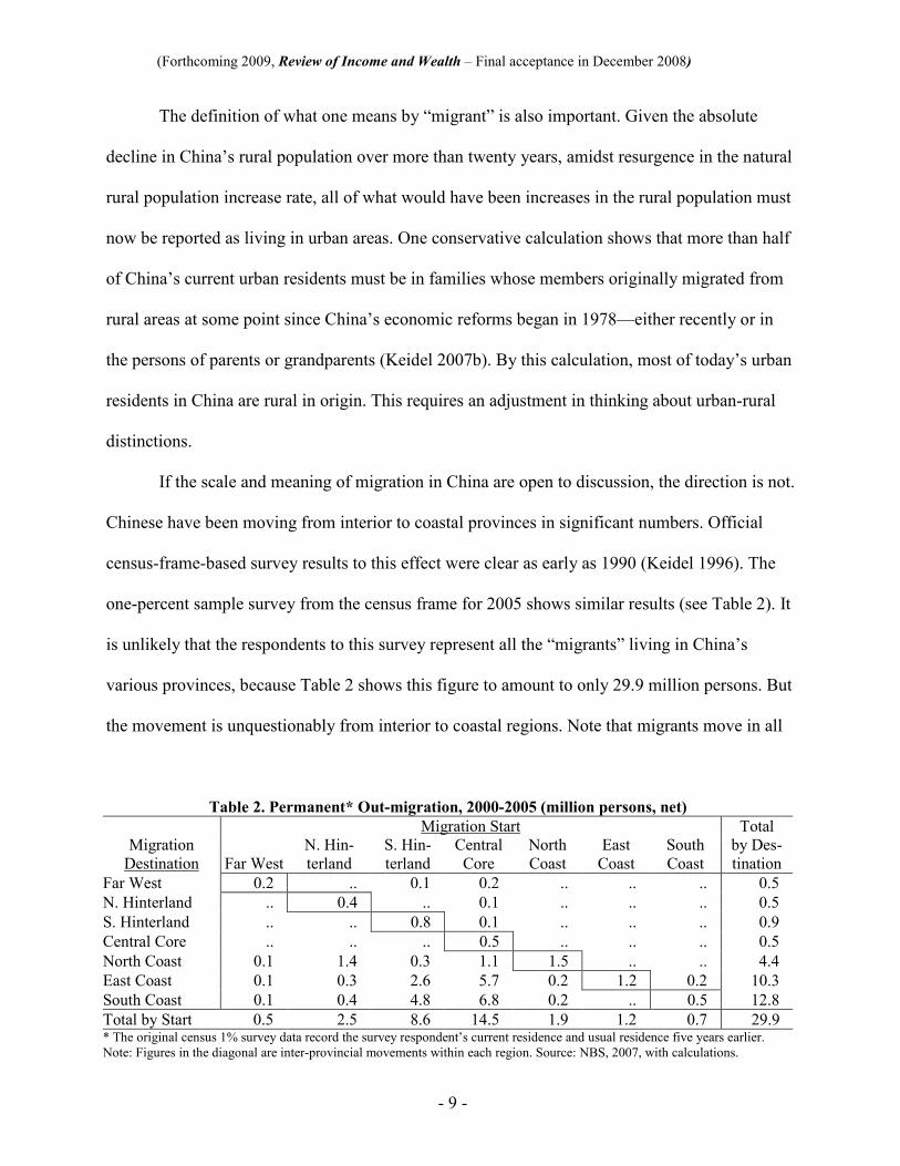
If the scale and meaning of migration in China are open to discussion, the direction is not.

Chinese have been moving from interior to coastal provinces in significant numbers. Official

census-frame-based survey results to this effect were clear as early as 1990 (Keidel 1996). The

one-percent sample survey from the census frame for 2005 shows similar results (see Table 2). It

is unlikely that the respondents to this survey represent all the “migrants” living in China’s

various provinces, because Table 2 shows this figure to amount to only 29.9 million persons. But

the movement is unquestionably from interior to coastal regions. Note that migrants move in all

Table 2. Permanent* Out-migration, 2000-2005 (million persons, net) Migration Start Total

Migration Destination Far West

N. Hin-terland

S. Hin-terland

Central Core

North Coast

East Coast

South Coast

by Des-tination

Far West 0.2 .. 0.1 0.2 .. .. .. 0.5 N. Hinterland .. 0.4 .. 0.1 .. .. .. 0.5 S. Hinterland .. .. 0.8 0.1 .. .. .. 0.9 Central Core .. .. .. 0.5 .. .. .. 0.5 North Coast 0.1 1.4 0.3 1.1 1.5 .. .. 4.4 East Coast 0.1 0.3 2.6 5.7 0.2 1.2 0.2 10.3 South Coast 0.1 0.4 4.8 6.8 0.2 .. 0.5 12.8 Total by Start 0.5 2.5 8.6 14.5 1.9 1.2 0.7 29.9 * The original census 1% survey data record the survey respondent’s current residence and usual residence five years earlier. Note: Figures in the diagonal are inter-provincial movements within each region. Source: NBS, 2007, with calculations.


- 10 -

directions, but on a net basis as calculated from this survey, coastal provinces had 27.5 million

persons who had permanently moved from other provinces during the five years through 2005.

The indicated direction of migration toward more productive regions implies an upward bias in

measured GDP-per-capita disparities.

One way of avoiding migration-induced measurement complications is to make

comparisons based on household survey data.

China’s household survey system is well developed and has been in place in its modern

form since the early 1980s. As we have seen, the surveys nevertheless pose significant research

challenges—in design, interpretation, and the general availability of data generated by the

surveys.

Since at least the early 1960s, China’s population has been divided into two matrilineal

categories, rural and urban—or as originally termed, “agricultural” and “non-agricultural.” A

Chinese citizen’s population registration status has traditionally been crucial to determining

educational, employment and social safety net opportunities—urban registered citizens were

educated in urban areas and could expect jobs in the modern non-farm sector. Rural registered

persons originally received none of these benefits—unless they could change their legal status

through educational performance or some other kind of promotion.

These household registration categories are currently going through rapid reform with a

goal to eliminating the distinction and with it the variance in subsidized privileges between the

two groups. But household survey instruments, originally designed to meet the different

circumstances of the two groups, continue with their basic differences.

The most fundamental survey distinction is between the rural household survey, designed

for families engaged in a family-owned business (i.e., farming), and a different, simpler survey


- 11 -

for urban families, traditionally characterized as wage-earning families. Both surveys use a well-

developed system of family ledgers and statistical workers who regularly check and assist with

the record keeping. Ironically, China’s dramatic reforms since 1978 have turned many rural

workers into wage earners and many urban households into sole proprietorships. The original

rationale for two separate survey instruments is thus no longer operational, and introduction of a

single unified household survey instrument is long overdue.

The rural survey’s business-oriented instrument has data on gross earnings from sales,

costs of production, and “net income,” which is household enterprise income minus production

costs and taxes, but including remittances from persons away from the home, government

transfers, interest income, and in-kind income from own-production—mostly food, in recent

years valued at close to local selling prices (Ravallion and Chen 2004). In 2007, 14 percent of

rural gross income and 14 percent of rural living expenditures were non-cash in nature (NBS

2008). This reported “net” income is basically a cash-basis calculation, except it does not include

borrowings and debt principal repayments to financial institutions or other creditors. This “net

income” measure is the basic income figure used for standard of living calculations for

households not registered as urban.

Consumption in the rural survey is from the reported summation of “Expenditures for

daily household living needs.” One of its most serious shortcomings is the lack of imputed rent

for owner-occupied rural housing while it generally includes home-improvement expenses more

appropriately considered to be investment outlays. There are also no corrections for interregional

cost of living indicators, and detailed data are too few to adjust for unreported scale advantages

enjoyed by large families sharing a house and its durables. Research on a subset of southern

Chinese provinces indicates that such shortcomings result in household survey statistics


- 12 -

overstating somewhat the actual degree

of regional inequality (Ravallion and

Chen 1998). A recent study by China’s

rural household survey team made a

different but related point, showing that

while pay for migrants from the interior

is higher on the coast than elsewhere,

when living costs are factored in,

migrants from the interior make less net income on the coast than do migrants who go to interior

locations (NBS 2005).

A main point to stress is that the “rural” designation for households covered by this part

of China’s household survey system is not a geographical designation at all, and neither is it an

agricultural designation, since many so-called rural persons work in cities for long periods of

time or engage in non-farm businesses or wage income in non-farm businesses in small-town and

suburban areas. Of course, most of “rural” China by this survey is indeed involved in agriculture

as was more than 40 percent of China’s workforce in 2005, but given its heterogeneous nature,

“rural household survey” is in many ways a misnomer.

Despite shortcomings, household survey data tell a great deal about regional inequality.

In income terms, rural households in China’s coastal regions—especially the East Coast region

centered on Shanghai—are far and away better remunerated than those in the interior. By 2005,

rural households in the relatively small East Coast region, with total population of 142 million

people, had at least double the rural income level of those in any interior region (see Table 3).

Table 3. Regional Real Per Capita Rural Income* (Constant 2000 Yuan)

1985 1990 1995 2000 2005 China Total 943 1,306 1,700 2,253 3,556 Far West 748 1,027 1,058 1,514 2,410 N. Hinterland 846 1,228 1,405 1,867 3,062 S. Hinterland 743 1,052 1,271 1,733 2,662 Central Core 879 1,141 1,476 2,083 3,218 North Coast 1,004 1,336 1,895 2,613 4,196 East Coast 1,258 2,007 2,940 3,879 6,404 South Coast 1,113 1,764 2,628 3,411 4,901 * Income is “Net” income (

��)

Source: NBS household survey data, published in 2006 China Yearbook of Rural Household Survey (in Chinese), China Statistics Press, 2006


- 13 -

Not only are income

disparities large, they have been

growing larger over time. On average

for both 1985-to-2005 and for 2000-

to-2005, the regions that were already

leading in terms of per-capita rural

income at the outset of the period also

grew faster in real terms during that period. The rankings for both levels and growth rates are the

same, implying divergence (see Tables 3 and 4). What is more, the differences in growth rates

are substantial. All of the interior regions sustained average growth between 6.0 and 6.7 percent

over the twenty years after 1985 (see Table 4). During this same period, coastal regions averaged

rural household real income growth rates between 7.4 and 8.5 percent, a growth gap that is

especially large when compounded over twenty years.

Both China’s regional rural income disparities and the pace of their increase appear more

clearly in log-normal plots of their twenty-year trends (see Figures 1 and 2), for which the slopes

of the lines represent growth rates. Figure 1 shows clearly that the highest-income regions in

1985 also grew the fastest on average to 2005.

Figure 2 shows, however, that this diverging path was not at all uniform during the four

5-year sub-periods. Indeed, there were periods of convergence between 1995 and 2000. This

short-lived convergence path is also clear from the growth rates in Table 4, which show that for

the five years ending in 2000, the two highest-income regions grew more slowly than all the

other regions. Regional rural income levels in the subsequent five-year period, ending in 2005,

Table 4. Regional Rural Income Growth* 1980-2005

Ave. annual % 1985 1990 1995 2000 2005 1985-2005

China Total 14.1 6.7 5.4 5.8 9.6 6.9 Far West n/a 6.5 0.6 7.4 9.7 6.0 N. Hinterland 13.0 7.7 2.7 5.9 10.4 6.6 S. Hinterland 10.7 7.2 3.8 6.4 9.0 6.6 Central Core 13.6 5.3 5.3 7.1 9.1 6.7 North Coast 14.4 5.9 7.2 6.6 9.9 7.4 East Coast 16.7 9.8 7.9 5.7 10.5 8.5 South Coast 12.4 9.6 8.3 5.4 7.5 7.7 * Annual averages - except for 1985-2005, data show averages of real growth over five years, e.g., 1985 is for 1980-85. Source: See Table 3.


- 14 -

are also not uniformly divergent, with growth rates for the South Coast in particular failing to

recover the way they did in the North and East Coast regions.

A detailed discussion of the causes of these trends is beyond the scope of this paper, but it

is important to note that the 1990s were more complicated than the overall trends indicate, with

relatively poor performances in particular during 1990-1995 for the lower-income regions of the

Far West and North Hinterland.

Switching from income to consumption inequality patterns and trends for rural household

provides evidence of weaker divergence and of possible difficulties in the latter 1990s not

apparent in income statistics. Overall, regional rural household consumption disparities are in

many ways similar to the income patterns already described, except that the disparities and rates

of divergence are somewhat lower, the North Coast region’s levels are more like those in interior

regions, and the 5-year growth patterns show substantially more difficulties for all regions in the

Figure 1. Twenty-year Income Divergence Figure 2. Five-year Income Divergence Paths

1985 2005

E. CoastS. CoastN. CoastCentral CoreN. HinterlandS. HinterlandFar West

Log Scale

6,404

4,901

4,196

3,556

3,218

3,0622,6622,410

Rural Household 1985-2005Real Per-capita Net Income(Constant 2000 Yuan)

8.5

7.77.4

6.76.66.6

6.0

1,258

1,1131,004879846748743

Per-capitaRuralIncome


Ave. Annual Real Growth Rate 1985-2000 (%)

1985 1990 1995 2000 2005

E. Coast

S. Coast

N. Coast

Central Core

N. Hinterland

S. Hinterland

Far West

Log Scale

6,404

4,901

4,196

3,2183,062

2,6622,410

Rural Household 1985-2005Real Per-capita Net Income(Constant 2000 Yuan)


8.5

7.7

7.4

6.7

6.6

6.6

6.0

1,258

1,1131,004879846748743


Per-capitaRural

Income

* Both income levels and growth are in real terms. Sources: for both figures, see Tables 3 and 4.


- 15 -

latter half of the 1990s. We will

see below that shifts in savings

rates offer important insights into

this consumption trend.

Despite the less dramatic

disparities and speeds of

divergence, the rankings of the regions are, not surprisingly, the same as those for income. The

East Coast and South Coast have average levels of rural household consumption so much higher

than those in other regions to be adequately accounted for by regional price differences (see

Table 6). Furthermore, even though the North Coast’s household consumption levels are much

closer to levels in the interior, especially if possible price differences are considered, they are

still higher, so that as a general conclusion the data show that all coastal regions enjoy rural

household consumption levels higher than those in the interior.

As mentioned at the outset of this paper, however, the striking pattern in regional rural

household consumption is for growth rates (see Table 5). In particular, while on average over 20

years real consumption growth rates are highest on the coast, confirming some degree of long-

term divergence, the 1990s exhibit dramatic slowing in the interior during the first half of the

decade and in all regions during the

second half. Secondly, while all

regions recovered rapid growth of

rural consumption during 2000-2005,

recovery in the South Coast region

was weaker, while growth in the

Table 5. Rural Consumption Growth* 1980-2005

Ave. annual % 1980-1985

1985-1990

1990-1995

1995-2000

2000-2005

1985-2005

China Total n/a 8.1 4.9 3.4 10.8 6.8 Far West n/a 6.6 4.7 3.1 11.9 6.5 N. Hinterland 10.8 8.2 4.3 2.3 11.4 6.5 S. Hinterland 11.0 8.0 4.1 3.6 10.3 6.5 Central Core 12.1 7.2 3.9 4.4 10.4 6.4 North Coast 14.0 6.1 5.9 3.3 11.4 6.6 East Coast 16.2 9.8 6.1 2.9 12.0 7.7 South Coast 11.7 11.9 7.0 2.4 8.7 7.4 * Annual averages; except for 1985-2005, data show averages of real growth over five years, e.g., 1985 is for 1980-85. Source: See Table 3.

Table 6. Regional Real Per Capita Rural Consumption* (Constant 2000 Yuan)

1985 1990 1995 2000 2005China Total 753 1,112 1,412 1,670 2,792Far West n/a 800 1,007 1,174 2,059N. Hinterland 675 1,003 1,238 1,384 2,369S. Hinterland 641 942 1,154 1,374 2,248Central Core 717 1,016 1,230 1,524 2,495North Coast 787 1,059 1,407 1,658 2,840East Coast 1,084 1,734 2,337 2,697 4,749South Coast 897 1,576 2,211 2,485 3,763Source: See Table 3.


- 16 -

interior basically matched rates in the North Coast and East Coast regions.

The levels, trends and variations in growth rates for household consumption by regions

are clearest in Figures 3 and 4. Long-term divergence is less than for income, and in the period

2000-2005, except for the South Coast, there is essentially neither divergence nor convergence.

Considering both income and consumption, however, real growth rates are so high, both

over twenty years and for the most recent five-year period, that issues of convergence or

divergence are arguably less important than they otherwise would be. All of rural China appears

to have improved dramatically its well being, as measured by consumption, since economic

reforms in the early 1980s broke up Maoist-era communes in favor of family farming.

These data for rural household income and consumption disparities, however, raise

questions about the usefulness of basing inequality and poverty analysis on consumption in

countries with rapid changes over time in household savings rates. Indeed, these data show just

such changes and interregional differences for all of China’s regions since the 1980s. Table 7

Figure 3. Rural Consumption* Divergence Figure 4. Consumption Divergence Paths

1985 2005

E. Coast

S. Coast

N. Coast

Central Core

N. Hinterland

S. Hinterland

Far West

Log Scale

4,749

3,763

2,840

2,4952,3692,2482,059

Rural Household 1985-2005Real Per-capita Consumption

(Constant 2000 Yuan)


1,084

897

787717675641583

Per-capitaRural

Consumption

Per-capitaRural

Consumption

7.77.4

6.6

6.4

6.5

6.5

6.5

1985 1990 1995 2000 2005

E. Coast

S. Coast

N. Coast

Central Core

N. Hinterland

S. Hinterland

Far West

Log Scale

Rural Household 1985-2005Real Per-capita Consumption

(Constant 2000 Yuan)

Ave. Annual Real Growth

Rate

7.77.4

6.6

6.4

6.5

6.5

6.5

1,084

897

787

717675

583641

Per-capitaRural

Consumption

4,749

3,763

2,8402,4952,369

2,0592,248

Per-capitaRural

Consumptio

* Both consumption levels and growth are in real terms. Sources: for both figures, see Tables 3 and 4.


- 17 -

shows the decline in savings

rates from the early 1980s to

the early 1990s (from the

period ending in 1985 to that

ending in 1995). Nationwide,

the population-weighted

average of provincial savings

rates (Total #2 in Table 7)

dropped from an average of

roughly 17 percent in 1980-85 to under 13 percent in 1990-95. But the decline was especially

sharp in the deep interior—the Hinterland and Far West regions—while savings rates actually

increased in coastal provinces during 1990-95.

Under such circumstances of rapidly shifting savings rates, how useful is it to compare

household well-being based in consumption—when consumption levels may be maintained

under income stress? Conversely, when savings rates soar, as they did for China’s rural

households in the latter 1990s (1995-2000), are resulting lower-than-otherwise consumption

levels accurate measures of the change in relative well-being? This may be the case, if higher

savings rates resulted from a sudden increase in uncertainty over costs of education, healthcare

and other necessities and such anxieties are considered important. In general, however, when

savings rates differ so much over time and between regions for the same period, such patterns

introduce doubts about interpretations of interregional gaps in household consumption and their

trends over time.

Table 7. Regional Rural Household Savings Rates , 1980-2005 1980 1985 1990 1995 2000 2005 China Total #1 n/a 20.2 14.8 16.9 25.9 21.5 China Total #2* n/a 16.5 13.6 12.7 22.6 17.1 Far West n/a 22.2 22.1 4.8 22.5 14.5 N. Hinterland 11.9 20.2 18.4 11.9 25.9 22.6 S. Hinterland 14.8 13.7 10.5 9.2 20.7 15.5 Central Core 12.9 18.5 11.0 16.7 26.8 22.4 North Coast 20.5 21.7 20.7 25.7 36.5 32.3 East Coast 12.1 13.8 13.6 20.5 30.5 25.8 South Coast 16.7 19.4 10.7 15.9 27.1 23.2 * Two different national savings rate calculations give substantially different answers. Total #1 is the ratio of national total rural household savings to national total rural household income; it gives greater weight to regional savings rates in the highest-income regions; Total #2 is a population-weighted average of individual provincial savings rates and hence is a better average of nationwide household savings behavior patterns. Sources: See Table 3.


- 18 -

Further inquiry into

distributional patterns of household

savings emphasizes concerns about

making consumption a standard for

assessing poverty levels in a region or a

country with rapidly shifting savings

rates. Based on a summary report (NBS

2000b) of both income and

consumption distribution information

for a subset of Chinese counties known as “poverty counties,” we can compare distributions and

savings rates by both measures in Table 8. Population shares are distributed as one would expect,

with larger shares of the population in each of the lower categories by the consumption measure

than by the income measure. This accords with the notion that typical households have lower

consumption levels than income levels.

The surprise in Table 8 is that low-consumption households have high average savings

rates. This contradicts the general understanding that poor households save less, often dissaving

to meet consumption needs. The income categories distribution shows just such a pattern in

Table 8. Here, poor households have negative savings rates.

What could explain the high savings rates for households with low average levels of

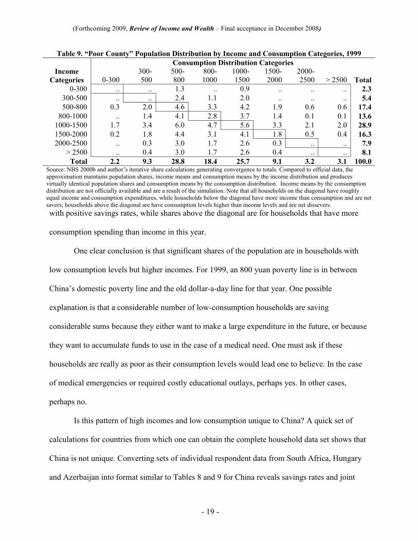
consumption? The joint distribution shown in Table 9 provides one indication. It shows the

population of China’s 1999 poor counties identified by both income and consumption levels.

Shares on the diagonal represent households with roughly equal income and consumption. They

have something close to a zero savings rate. Shares below the diagonal represent households

Table 8. “Poor County” Population Distributions by Income and Consumption, with Savings Rates, 1999

(percent) Sorted by: Income Consumption Chinese RMB yuan

Population Share

Savings Rate

Population Share

Savings Rate

0-300 2.3 -244.0 2.2 73.7 300-500 5.4 -58.4 9.3 52.0 500-800 17.4 -8.8 28.8 36.5 800-1000 13.6 5.0 18.4 28.5 1000-1500 28.9 18.5 25.7 21.0 1500-2000 16.3 29.1 9.1 12.3 2000-2500 7.9 35.9 3.2 3.6

> 2500 8.1 45.3 3.1 -33.3 Total 100.0 22.7 100.0 22.7

Source: NBS 2000b and author simulations and calculations; see note to Table 9. Savings rates as a percent are the ratios of average income levels consumption expenditure levels, minus one.


- 19 -

with positive savings rates, while shares above the diagonal are for households that have more

consumption spending than income in this year.

One clear conclusion is that significant shares of the population are in households with

low consumption levels but higher incomes. For 1999, an 800 yuan poverty line is in between

China’s domestic poverty line and the old dollar-a-day line for that year. One possible

explanation is that a considerable number of low-consumption households are saving

considerable sums because they either want to make a large expenditure in the future, or because

they want to accumulate funds to use in the case of a medical need. One must ask if these

households are really as poor as their consumption levels would lead one to believe. In the case

of medical emergencies or required costly educational outlays, perhaps yes. In other cases,

perhaps no.

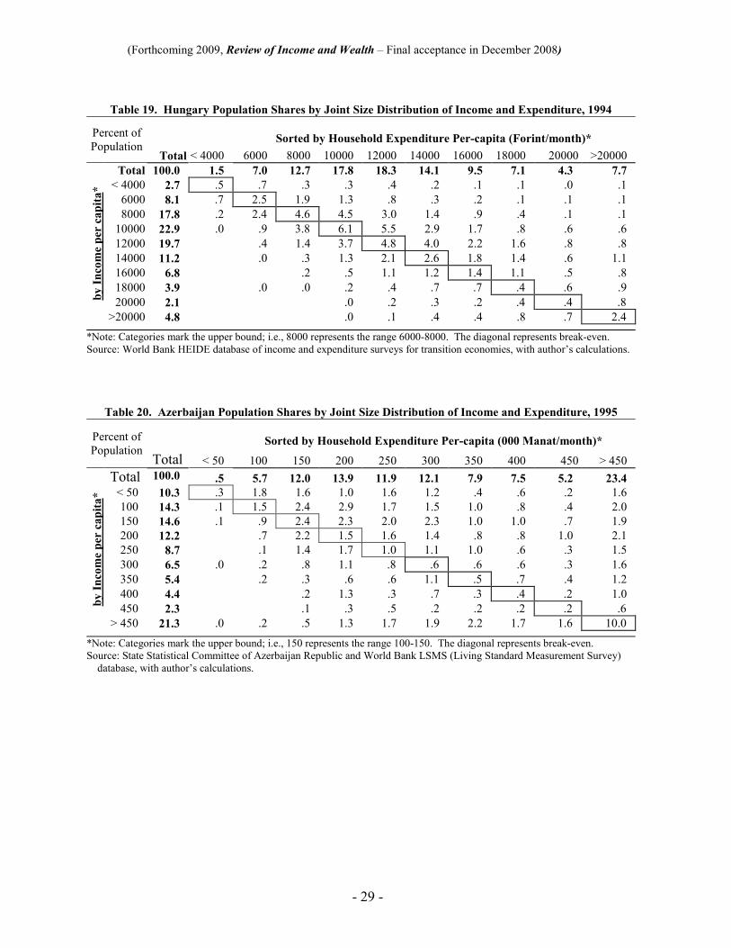
Is this pattern of high incomes and low consumption unique to China? A quick set of

calculations for countries from which one can obtain the complete household data set shows that

China is not unique. Converting sets of individual respondent data from South Africa, Hungary

and Azerbaijan into format similar to Tables 8 and 9 for China reveals savings rates and joint

Table 9. “Poor County” Population Distribution by Income and Consumption Categories, 1999 Consumption Distribution Categories Income

Categories 0-300 300-500

500-800

800-1000

1000-1500

1500-2000

2000-2500 > 2500 Total

0-300 .. .. 1.3 .. 0.9 .. .. .. 2.3 300-500 .. .. 2.4 1.1 2.0 .. .. .. 5.4 500-800 0.3 2.0 4.6 3.3 4.2 1.9 0.6 0.6 17.4 800-1000 .. 1.4 4.1 2.8 3.7 1.4 0.1 0.1 13.6 1000-1500 1.7 3.4 6.0 4.7 5.6 3.3 2.1 2.0 28.9 1500-2000 0.2 1.8 4.4 3.1 4.1 1.8 0.5 0.4 16.3 2000-2500 .. 0.3 3.0 1.7 2.6 0.3 .. .. 7.9

> 2500 .. 0.4 3.0 1.7 2.6 0.4 .. .. 8.1 Total 2.2 9.3 28.8 18.4 25.7 9.1 3.2 3.1 100.0

Source: NBS 2000b and author’s iterative share calculations generating convergence to totals. Compared to official data, the approximation maintains population shares, income means and consumption means by the income distribution and produces virtually identical population shares and consumption means by the consumption distribution. Income means by the consumption distribution are not officially available and are a result of the simulation. Note that all households on the diagonal have roughly equal income and consumption expenditures, while households below the diagonal have more income than consumption and are net savers; households above the diagonal are have consumption levels higher than income levels and are net dissevers.


- 20 -

income-consumption distribution patterns essentially similar to China’s. See Tables 17, 18, 19,

and 20 in the statistical appendix. All three countries show negative average savings rates for

households in low income categories, but significantly high positive average savings rates for

households in low consumption categories.

A final consideration regarding regional inequality is the incidence of poverty in different

regions, and in particular differences in the incidence of poverty in coastal and interior areas.

Comparisons between the seven aggregated regions introduced earlier are beyond the scope of

this research, in part because not all provinces publish household income size distribution

statistics. Comparisons for five representative provinces, however, illustrate both the level of

differences and the importance of using a relevant poverty line for measuring inequality and

informing policy making.

In December 2007 the World Bank’s released revised purchasing power parity (PPP)

conversion factors for the world, including China (World Bank 2007b and 2007c). An

appropriate poverty line for regional comparisons within China is potentially one of three

choices: the domestic Chinese poverty line, the newly revised PPP one-dollar-a-day poverty line,

and the newly revised two-dollar-a-day line. These three poverty line standards for 2005, along

with the old dollar-a-day poverty line for comparison, are presented in Table 10. Analysis below

shows that of the three, the revised one-dollar-a-day standard is best for making interregional

comparisons.

Using the World Bank’s PovCal facility for

estimating China’s national consumption-based size

distribution, and based on estimates of the new PPP

dollar-a-day poverty standard consistent with the

Table 10. 2005 China Poverty Lines (Annual levels) US$* Yuan*

Chinese Poverty Line 83 683 Old PPP $1/day Line 117 955 New PPP $1/day Line 201 1,649 New PPP $2/day Line 403 3,298 * US$ at 2005 average commercial exchange rate;

Yuan are 2005 yuan. Sources: World Bank 2007a, 2007b, NBS 2007, with

calculations


- 21 -

new World Bank PPP statistics, China’s consumption-based dollar-a-day poverty incidence is

roughly 300 million rural persons, compared to roughly 100 million using the old dollar-a-day

standard (Keidel 2007c).

There are, however, no available consumption-based distribution data for individual

provinces, limiting poverty comparisons to those based on income-based rather than

consumption-based distribution data. Given China’s relatively high household savings rates,

most households have significantly higher incomes than consumption levels, so many fewer

households fall under an income dollar-a-day standard than under a dollar-a-day consumption

standard. For China as a whole, the difference for 2005 is roughly between 300 million poor by a

consumption dollar-a-day poverty standard and 100 million poor by an income dollar-a-day

standard. In light of the potential disadvantages of using consumption-based distribution data,

the good availability of income-based distribution data perhaps not a handicap after all.

Table 11 shows poverty incidence comparisons between five provinces for four different

poverty-line standards. Jiangsu and Liaoning are both coastal provinces, but while Jiangsu is part

of greater Shanghai and the dynamic East Coast region, Liaoning is part of Manchuria and has a

significant portion of its rural population living on difficult interior terrains with long winters.

Hunan is a quintessential grain-base province in China’s Central Core region, while Sichuan

(representing the South Hinterland region) and Shaanxi (in the North Hinterland region) are even

Table 11. Income Poverty Comparisons, Selected Chinese Provinces, 2005 (% of rural population) Jiangsu Liaoning Hunan Sichuan Shaanxi Total* All China* Chinese Poverty Line 0.7 4.2 1.1 7.6 5.6 4.2 2.9 Old PPP $1/day Line 1.8 5.9 4.8 13.4 11.7 8.2 4.0 New PPP $1/day Line 6.1 18.1 14.9 28.9 45.1 22.1 13.7 New PPP $2/day Line 33.4 55.4 59.7 75.8 87.6 63.1 47.1 * "Total" is for the five provinces; "All China" is for China's 2005 rural population Sources: NBS 2006 Provincial yearbooks for each province, NBS China Statistical Yearbook 2007, Dikhanov 1999, and

calculations. Note: Results are rough approximations because of the likelihood that PPP price comparisons for China as a whole are not accurately representative of price comparisons and income weights of poor household budget patterns. Nevertheless, the general orders of magnitude are almost certain to reflect actual provincial poverty differences.


- 22 -

more isolated. It is clear that the new dollar-a-day poverty standard reveals higher poverty levels

across the board, but the percentage-point gap it reveals between Jiangsu and all the other

provinces shown is substantial.

This poverty-based measure of regional disparities is arguably the most accurate gauge of

inter-regional differences in well-being, because regardless of the speed of improvement in

income and consumption in a poorer region, the scale of those left in absolute poverty is an

irreducible index of the degree to which the most basic household expectations remain unmet.

Table 12 presents the same comparisons of provincial poverty in terms of millions of

rural citizens. This head-count comparison supports conclusions similar to the incidence data in

Table 11 – the thriving coastal provinces, represented by Jiangsu, have substantially lower

numbers of poor people, especially by the new dollar-a-day measure. It is important to

emphasize, therefore, that the choice of an appropriate poverty-line standard is crucial for using

poverty data to assess inter-regional differences in well being. Too high a poverty line, like the

new two-dollar-a-day standard, tends to hide meaningful interregional disparities. These points

are reinforced by review of the different provincial distributions presented in Figure 5.

This concludes the brief introduction to regional inequality in rural China. To summarize,

disparities are large, with rural household income and consumption on average much higher in

coastal provinces than in the interior. What is more, the gap is widening—especially for

incomes. The sustained high rates of improvement in all regions over twenty years, however,

Table 12. Income Poverty Comparisons, Selected Chinese Provinces, 2005 (million rural persons) Jiangsu Liaoning Hunan Sichuan Shaanxi Total* All China* Chinese Poverty Line 0.3 0.9 0.5 5.0 1.3 8.0 21.8 Old PPP $1/day Line 0.7 1.3 2.0 8.9 2.7 15.6 29.9 New PPP $1/day Line 2.3 3.9 6.3 19.1 10.5 42.2 103.0 New PPP $2/day Line 12.3 12.0 25.3 50.2 20.5 120.3 354.0 Rural Population 37.0 21.6 42.4 66.3 23.4 190.6 751.2 Sources and notes: see Table 11.


- 23 -

heavily qualify the seriousness of these gaps for making comparisons in well being. The rapid

increases in savings rates, especially in the late 1990s, casts serious doubts about using

consumption levels as a measure of changes in well being over time. A shift to slower

consumption growth while income growth continues at a more rapid pace appears to reflect

increased savings activity on the part of the non-poor as they take advantage of medium-term

savings programs intended to enable significant lumpy expenditures one or more years hence. A

more meaningful measure of regional differences in well being is arguably the incidence of

absolute poverty in different provinces, especially when measured with a policy line appropriate

for China in the first decade of the twenty-first century.

Figure 5. Rural Income Poverty Incidence for selected Provinces, 2005

0

2

4

6

8

10

12

0

60

120

180

240

310

370

430

490

550

610

670

730

790

850

920

980

Jiangsu

Liaoning

Hunan

Sichuan

Shaanxi

Rural Population % per $31interval

Old PPP $/day

Chinese Poverty Line

Constant 2005 US$ per capita annual net income (at 2005 exchange rate, rounded)

New PPP $1/day

New PPP $2/day

Note: for discussion of the “New PPP $1/day and $2/day poverty lines, see note for Figure Error! Bookmark not defined.. Sources: see Table 12.


- 24 -

Statistical Appendix

Table 13 – Regional Population and GDP Comparisons, 2005 Population Total GDP Per capita Sector Shares (%) (million) (Bil.US$*) GDP ($) Primary Secondary Tertiary China Total 1,308 2,246 1,717 12.5 47.3 40.2 Far West 60 72 1,204 16.9 44.0 39.1 Xinjiang 20 32 1,582 19.6 44.7 35.7 Tibet 3 3 1,107 19.1 25.3 55.6 Qinghai 5 7 1,221 12.0 48.7 39.3 Gansu 26 24 910 15.9 43.4 40.7 Ningxia 6 7 1,241 11.9 46.4 41.7 N. Hinterland 160 255 1,594 12.4 50.4 37.2 Heilongjiang 38 67 1,761 12.4 53.9 33.7 Jilin 27 44 1,627 17.3 43.6 39.1 Inner Mongolia 24 48 1,993 15.1 45.5 39.4 Shanxi 34 51 1,521 6.3 56.3 37.4 Shaanxi 37 45 1,206 11.9 50.3 37.8 S. Hinterland 239 244 1,023 19.5 40.5 40.0 Greater Sichuan 110 128 1,159 18.6 41.4 40.0 Guizhou 37 24 648 18.6 41.8 39.6 Yunnan 45 42 953 19.3 41.2 39.5 Guangxi 47 50 1,068 22.4 37.1 40.5 Central Core 318 403 1,267 18.0 45.6 36.4 Henan 94 129 1,378 17.9 52.1 30.0 Anhui 61 66 1,072 18.0 41.3 40.7 Jiangxi 43 50 1,149 17.9 47.3 34.8 Hubei 57 80 1,394 16.6 43.1 40.3 Hunan 63 79 1,257 19.6 39.9 40.5 North Coast 229 576 2,516 9.7 50.6 39.7 Liaoning 42 98 2,316 11.0 49.4 39.6 Greater Hebei 94 252 2,677 8.3 45.0 46.7 Shandong 92 226 2,444 10.6 57.4 32.0 East Coast 142 499 3,528 6.0 53.8 40.3 Greater Jiangsu 93 335 3,623 5.6 53.9 40.4 Zhejiang 49 164 3,349 6.6 53.4 40.0 South Coast 236 648 2,749 8.6 49.5 41.9 Fujian 35 80 2,268 12.8 48.7 38.5 Greater Guangdong 100 284 2,833 7.4 49.7 42.9 * US$ figures at 2005 average commercial exchange rate of 8.1917 Yuan/$. Source: China National Bureau of Statistics (NBS) 2006 Statistical Yearbook, with calculations


- 25 -

Table 14. “Greater” Provincial Real Rural Household Per-capita Income Levels, 1980-2005

2000 Constant Yuan 1980 1985 1990 1995 2000 2005 China Total 488 943 1,306 1,700 2,253 3,556 Far West n/a 748 1,027 1,058 1,514 2,410 Xinjiang 505 935 1,300 1,224 1,618 2,712 Tibet n/a 837 1,236 1,293 1,331 2,270 Qinghai n/a 814 1,065 1,110 1,491 2,351 Gansu 391 605 820 948 1,429 2,163 Ningxia 455 762 1,100 1,076 1,724 2,741 N. Hinterland 459 846 1,228 1,405 1,867 3,062 Heilongjiang 524 943 1,446 1,903 2,148 3,519 Jilin 603 981 1,529 1,734 2,023 3,566 Inner Mongolia 463 855 1,155 1,302 2,038 3,265 Shanxi 398 850 1,148 1,302 1,906 3,158 Shaanxi 364 700 1,010 1,037 1,444 2,242 S. Hinterland 447 743 1,052 1,271 1,733 2,662 Greater Sichuan 480 747 1,061 1,248 1,901 3,064 Guizhou 412 683 828 1,171 1,374 2,051 Yunnan 383 802 1,029 1,089 1,479 2,231 Guangxi 443 719 1,217 1,558 1,865 2,725 Central Core 464 879 1,141 1,476 2,083 3,218 Henan 410 781 1,003 1,327 1,986 3,136 Anhui 472 876 1,026 1,404 1,935 2,885 Jiangxi 462 895 1,274 1,656 2,135 3,418 Hubei 434 999 1,276 1,628 2,269 3,386 Hunan 561 938 1,264 1,536 2,197 3,406 North Coast 513 1,004 1,336 1,895 2,613 4,196 Liaoning 697 1,110 1,591 1,892 2,356 4,032 Greater Hebei 487 1,005 1,293 1,952 2,655 4,151 Shandong 496 968 1,294 1,848 2,659 4,294 East Coast 582 1,258 2,007 2,940 3,879 6,404 Greater Jiangsu 595 1,237 1,966 2,779 3,681 5,925 Zhejiang 559 1,301 2,091 3,196 4,254 7,276 South Coast 621 1,113 1,764 2,628 3,411 4,901 Fujian 438 940 1,454 2,207 3,231 4,862 Greater Guangdong 700 1,175 1,928 2,809 3,495 4,919 Note: Greater Sichuan combines Sichuan and Chongqing; Greater Hebei combines Hebei, Beijing and Tianjin; Greater Guangdong combines Guangdong and Hainan.


- 26 -

Table 15. “Greater” Provincial Real Rural Household Per-capita Consumption Levels, 1980-2005

2000 Constant Yuan 1980 1985 1990 1995 2000 2005 China Total n/a 753 1,112 1,412 1,670 2,792 Far West n/a 583 800 1,007 1,174 2,059 Xinjiang 384 689 964 1,014 1,236 2,102 Tibet n/a 639 934 966 1,117 1,883 Qinghai n/a 652 903 985 1,218 2,159 Gansu 323 485 646 986 1,084 1,988 Ningxia 346 629 920 1,146 1,417 2,288 N. Hinterland 405 675 1,003 1,238 1,384 2,369 Heilongjiang 419 727 1,114 1,594 1,540 2,780 Jilin 552 865 1,204 1,610 1,553 2,519 Inner Mongolia 400 691 936 1,272 1,615 2,673 Shanxi 343 647 928 1,000 1,149 2,051 Shaanxi 357 554 908 984 1,251 2,072 S. Hinterland 381 641 942 1,154 1,374 2,248 Greater Sichuan 407 655 969 1,178 1,462 2,453 Guizhou 357 604 767 1,003 1,097 1,696 Yunnan 318 633 924 1,057 1,271 1,955 Guangxi 386 636 1,022 1,296 1,488 2,567 Central Core 404 717 1,016 1,230 1,524 2,495 Henan 346 616 833 1,001 1,316 2,067 Anhui 416 709 980 1,153 1,322 2,399 Jiangxi 398 719 1,098 1,353 1,643 2,713 Hubei 390 794 1,156 1,341 1,556 2,655 Hunan 492 827 1,158 1,473 1,943 3,011 North Coast 408 787 1,059 1,407 1,658 2,840 Liaoning 582 953 1,292 1,586 1,754 3,065 Greater Hebei 394 760 997 1,302 1,512 2,599 Shandong 372 764 1,041 1,442 1,771 2,989 East Coast 512 1,084 1,734 2,337 2,697 4,749 Greater Jiangsu 525 1,065 1,702 2,195 2,415 4,098 Zhejiang 490 1,124 1,800 2,563 3,231 5,936 South Coast 517 897 1,576 2,211 2,485 3,763 Fujian 402 832 1,347 1,933 2,410 3,597 Greater Guangdong 567 920 1,697 2,331 2,520 3,839 Note: Greater Sichuan combines Sichuan and Chongqing; Greater Hebei combines Hebei, Beijing and Tianjin; Greater Guangdong combines Guangdong and Hainan.


- 27 -

Table 16 – “Greater” Provincial Rural Household Savings Rates, 1980-2005 2000 Constant Yuan 1980 1985 1990 1995 2000 2005

China Total 20.2 14.8 16.9 25.9 21.5 Far West 22.2 22.1 4.8 22.5 14.5 Xinjiang 23.9 26.4 25.9 17.1 23.6 22.5 Tibet 23.6 24.5 25.3 16.1 17.0 Qinghai 19.9 15.2 11.3 18.3 8.2 Gansu 17.4 19.8 21.3 -4.0 24.1 8.1 Ningxia 23.9 17.4 16.3 -6.4 17.8 16.5 N. Hinterland 11.9 20.2 18.4 11.9 25.9 22.6 Heilongjiang 20.1 22.9 22.9 16.2 28.3 21.0 Jilin 8.5 11.9 21.2 7.1 23.2 29.4 Inner Mongolia 13.6 19.2 19.0 2.3 20.8 18.2 Shanxi 13.7 23.9 19.2 23.2 39.7 35.0 Shaanxi 1.9 21.0 10.1 5.1 13.3 7.6 S. Hinterland 14.8 13.7 10.5 9.2 20.7 15.5 Greater Sichuan 15.2 12.3 8.7 5.6 23.1 19.9 Guizhou 13.4 11.5 7.3 14.4 20.2 17.3 Yunnan 17.0 21.1 10.2 3.0 14.1 12.4 Guangxi 13.0 11.5 16.0 16.8 20.2 5.8 Central Core 12.9 18.5 11.0 16.7 26.8 22.4 Henan 15.7 21.2 16.9 24.6 33.7 34.1 Anhui 11.9 19.1 4.5 17.8 31.7 16.8 Jiangxi 13.8 19.7 13.8 18.3 23.1 20.6 Hubei 10.1 20.6 9.4 17.6 31.4 21.6 Hunan 12.2 11.8 8.4 4.1 11.6 11.6 North Coast 20.5 21.7 20.7 25.7 36.5 32.3 Liaoning 16.4 14.2 18.8 16.2 25.6 24.0 Greater Hebei 19.1 24.4 22.9 33.3 43.1 37.4 Shandong 24.9 21.1 19.6 22.0 33.4 30.4 East Coast 12.1 13.8 13.6 20.5 30.5 25.8 Greater Jiangsu 11.9 13.9 13.4 21.0 34.4 30.8 Zhejiang 12.5 13.6 13.9 19.8 24.0 18.4 South Coast 16.7 19.4 10.7 15.9 27.1 23.2 Fujian 8.2 11.6 7.4 12.4 25.4 26.0 Greater Guangdong 19.0 21.7 12.0 17.0 27.9 22.0 Note: Greater Sichuan combines Sichuan and Chongqing; Greater Hebei combines Hebei, Beijing and Tianjin; Greater Guangdong combines Guangdong and Hainan.


- 28 -

Table 17. Comparisons of Savings Rates by Income and Consumption Sorts for Three Countries

Income Distribution Savings Rates (%) Consumption Distribution Savings Rates (%)

Income Groups

South Africa Hungary

Azer-baijan

Consumption Groups

South Africa Hungary

Azer-baijan

Lowest -668.5 -196.6 -844.7 Lowest 63.4 28.1 59.9 2 -133.2 -47.5 -267.7 2 29.8 19.3 45.2 3 -58.4 -29.2 -132.5 3 4.9 10.5 28.1 4 -26.3 -20.5 -78.6 4 -11.3 .2 31.7 5 -5.8 -13.7 -31.5 5 -18.0 -9.0 13.4 6 8.3 -9.6 -18.3 6 -37.9 -12.6 5.4 7 19.3 -.7 -12.8 7 -53.9 -22.5 18.4 8 24.9 1.4 4.7 8 -58.9 -25.7 .8 9 32.9 2.6 10.8 9 -79.6 -26.3 -4.6

Highest 37.7 17.0 50.8 Highest -93.0 -39.1 -7.4 National Average -25.4 -12.7 5.2 National Average -25.4 -12.7 5.2 Sources: See Tables 18, 19 and 20.

Table 18. South Africa Population Shares by Joint Size Distribution of Income and Expenditure, 1994

Percent of Population

Sorted by Household Expenditure Per-capita (Rand /month)* Total < 400 800 1200 1600 2000 2400 2800 3200 3600 >3600

by Incom

e per capita*

Total 100.0 3.6 18.3 20.8 18.1 12.2 9.0 6.5 5.1 3.8 2.5 < 400 21.4 1.2 6.3 5.1 3.8 1.8 1.2 .8 .6 .4 .2 800 23.2 1.3 5.1 5.8 4.0 2.5 1.8 1.3 .6 .3 .4 1200 16.5 .5 3.2 3.8 3.3 1.6 1.4 1.0 .6 .6 .3 1600 11.5 .2 1.6 2.4 2.5 1.4 1.2 .6 .9 .5 .3 2000 7.7 .2 .7 1.4 1.5 1.6 .7 .6 .5 .2 .3 2400 6.5 .1 .6 1.0 1.2 1.0 1.0 .5 .4 .5 .3 2800 4.8 .1 .4 .5 .8 .9 .6 .5 .4 .3 .2 3200 3.7 .1 .2 .5 .4 .6 .5 .4 .4 .5 .2 3600 2.5 .2 .2 .5 .4 .5 .3 .2 .2 .2 >3600 2.4 .1 .2 .2 .4 .3 .3 .4 .3 .2

*Note: Categories mark the upper bound; i.e., 1200 represents the range 800-1200. The diagonal generally represents break-even (i.e., income roughly equal to expenditure) except for the highest and lowest categories.

Source: National Statistical Office of South Africa and World Bank LSMS (Living Standard Measurement Survey) database, with author calculations.


- 29 -

Table 19. Hungary Population Shares by Joint Size Distribution of Income and Expenditure, 1994


Sorted by Household Expenditure Per-capita (Forint/month)* Total < 4000 6000 8000 10000 12000 14000 16000 18000 20000 >20000

by Incom

e per capita*

Total 100.0 1.5 7.0 12.7 17.8 18.3 14.1 9.5 7.1 4.3 7.7 < 4000 2.7 .5 .7 .3 .3 .4 .2 .1 .1 .0 .1 6000 8.1 .7 2.5 1.9 1.3 .8 .3 .2 .1 .1 .1 8000 17.8 .2 2.4 4.6 4.5 3.0 1.4 .9 .4 .1 .1 10000 22.9 .0 .9 3.8 6.1 5.5 2.9 1.7 .8 .6 .6 12000 19.7 .4 1.4 3.7 4.8 4.0 2.2 1.6 .8 .8 14000 11.2 .0 .3 1.3 2.1 2.6 1.8 1.4 .6 1.1 16000 6.8 .2 .5 1.1 1.2 1.4 1.1 .5 .8 18000 3.9 .0 .0 .2 .4 .7 .7 .4 .6 .9 20000 2.1 .0 .2 .3 .2 .4 .4 .8 >20000 4.8 .0 .1 .4 .4 .8 .7 2.4

*Note: Categories mark the upper bound; i.e., 8000 represents the range 6000-8000. The diagonal represents break-even. Source: World Bank HEIDE database of income and expenditure surveys for transition economies, with author’s calculations.

Table 20. Azerbaijan Population Shares by Joint Size Distribution of Income and Expenditure, 1995


Sorted by Household Expenditure Per-capita (000 Manat/month)*

Total < 50 100 150 200 250 300 350 400 450 > 450

by Incom

e per capita*

Total 100.0 .5 5.7 12.0 13.9 11.9 12.1 7.9 7.5 5.2 23.4 < 50 10.3 .3 1.8 1.6 1.0 1.6 1.2 .4 .6 .2 1.6 100 14.3 .1 1.5 2.4 2.9 1.7 1.5 1.0 .8 .4 2.0 150 14.6 .1 .9 2.4 2.3 2.0 2.3 1.0 1.0 .7 1.9 200 12.2 .7 2.2 1.5 1.6 1.4 .8 .8 1.0 2.1 250 8.7 .1 1.4 1.7 1.0 1.1 1.0 .6 .3 1.5 300 6.5 .0 .2 .8 1.1 .8 .6 .6 .6 .3 1.6 350 5.4 .2 .3 .6 .6 1.1 .5 .7 .4 1.2 400 4.4 .2 1.3 .3 .7 .3 .4 .2 1.0 450 2.3 .1 .3 .5 .2 .2 .2 .2 .6

> 450 21.3 .0 .2 .5 1.3 1.7 1.9 2.2 1.7 1.6 10.0 *Note: Categories mark the upper bound; i.e., 150 represents the range 100-150. The diagonal represents break-even. Source: State Statistical Committee of Azerbaijan Republic and World Bank LSMS (Living Standard Measurement Survey) database, with author’s calculations.


- 30 -

Bibliography Barboza, David, 2004, “Sharp Labor Shortage in China May Lead to World Trade Shift,” New

York Times, April 3, 2006. Cai, Fang, 2007, “Employment in China,” Presentation at session 1B of Asian Employment

Forum: Growth, Employment and Decent Work, held on Aug. 12 � 14, 2007, Beijing http://blog.voc.com.cn/sp1/caifang/075455363634.shtml

Ravallion and Chen 1998, Martin Ravallion and Shaohua Chen, "When Economic Reform is Faster than Statistical Reform: Measuring and Explaining Income Inequality in Rural China," World Bank Policy Research Working Paper Series, Paper No. 1902

Dikhanov, Yuri, 1999 GiniToolPak size distribution data manipulation software package (a Quasi-exact interpolation—exact on the nodes and accurate up to the second derivative between nodes), Rev. 1999, used with permission.

Horioka and Wan, 2007, Horioka, Charles Yuji and Junmin Wan, “The Determinants of Household Saving in China: A Dynamic Panel Analysis of Provincial Data,” Federal Reserve Bank of San Francisco Working Paper 2007-28, January

Keidel, Albert, 1994, China: GNP per Capita, unpublished (gray-cover) report for the World Bank, Report No. 13580-CHA.

Keidel, Albert, 1996, China’s Regional Disparities, unpublished draft (white-cover) consulting report for the World Bank.

Keidel, Albert, 2007a, “China’s Financial Sector: Contributions to Growth and Downside Risks,” Paper delivered at the conference China's Changing Financial System: Can it Catch Up With or Even Drive Economic Growth?, Networks Financial Institute, Indiana State University, January. http://www.carnegieendowment.org/files/keidel_china_financial_system.pdf

Keidel, Albert, 2007b, China’s Economic Fluctuations: Impact on the Rural Economy, December 2007, Washington, D.C.: Carnegie Endowment for International Peace. http://www.carnegieendowment.org/files/keidel_report_final.pdf .

Keidel, Albert, 2007c, “The Limits of a Smaller, Poorer China,” Financial Times, November 14, 2007, http://www.carnegieendowment.org/publications/index.cfm?fa=view&id=19709&prog=zch

Modigliani and Cao, 2004, Franco Modigliani and Shi Larry Cao, “The Chinese Saving Puzzle and the Life-Cycle Hypothesis,” Journal of Economic Literature, Vol. XLII (March 2004) pp. 145-170

NBS 2000a, China National Bureau of Statistics, China Rural Household Survey Yearbook 2000, Beijing: China Statistics Press

NBS 2000b, China National Bureau of Statistics, China Rural Poverty Monitoring Report 2000, Beijing: China Statistics Press

NBS 2005, China National Bureau of Statistics, Department of Rural Surveys, “Scale, Structure

and Special Characteristics of the Rural Migrant Labor Force” (�� ) in 2005 Research on Rural Labor of China (2005 ��), pp. 75-81

NBS 2006, China National Bureau of Statistics, China Rural Household Survey Yearbook 2006

(2006 ��), Beijing: China Statistics Press NBS 2007, China National Bureau of Statistics, 2005 National Population Census 1% Survey,

Beijing: China Statistics Press

http://blog.voc.com.cn/sp1/caifang/075455363634.shtml

http://www.carnegieendowment.org/files/keidel_china_financial_system.pdf

http://www.carnegieendowment.org/files/keidel_report_final.pdf

http://www.carnegieendowment.org/publications/index.cfm?fa=view&id=19709&prog=zch


- 31 -

NBS 2007b, China National Bureau of Statistics, China Statistical Abstract 2007 (Zhongguo tongji Zhaiyao 2007, in Chinese), Beijing: China Statistics Press

NBS 2008, China National Bureau of Statistics, China Statistical Yearbook, various years through 2008, Beijing: China Statistics Press

NBS Provincial, China National Bureau of Statistics, China provincial statistical yearbooks, for various years and various provinces (autonomous regions, etc.)

Ravallion, Martin and Shaohua Chen, 2004, “Understanding China’s (uneven) progress against poverty,” Finance and Development, December, pp. 16-19.

World Bank 1992. China: Statistical System in Transition, World Bank, Washington DC. World Bank 2007a, World Development Indicators 2007, Washington, D.C.: The World Bank. World Bank 2007b, 2005 International Comparison Program: Preliminary Results, December 17,

2005 http://siteresources.worldbank.org/ICPINT/Resources/ICPreportprelim.pdf World Bank 2007c, Press Release December 17, 2007: 2005 International Comparison Program

Preliminary Global Report compares Size of Economies http://go.worldbank.org/YM8TLUL8E0

World Bank, current, “POVCAL, A Program for Calculating Poverty Measures from Grouped Data,” http://www.worldbank.org/html/prdph/lsms/tools/povcal/

http://siteresources.worldbank.org/ICPINT/Resources/ICPreportprelim.pdf

http://go.worldbank.org/YM8TLUL8E0

http://www.worldbank.org/html/prdph/lsms/tools/povcal/

chinese regional inequalities in income and well-being - carnegie

Documents