choice

1

Choice

Molly W. DahlGeorgetown UniversityEcon 101 – Spring 2009

2

Economic Rationality

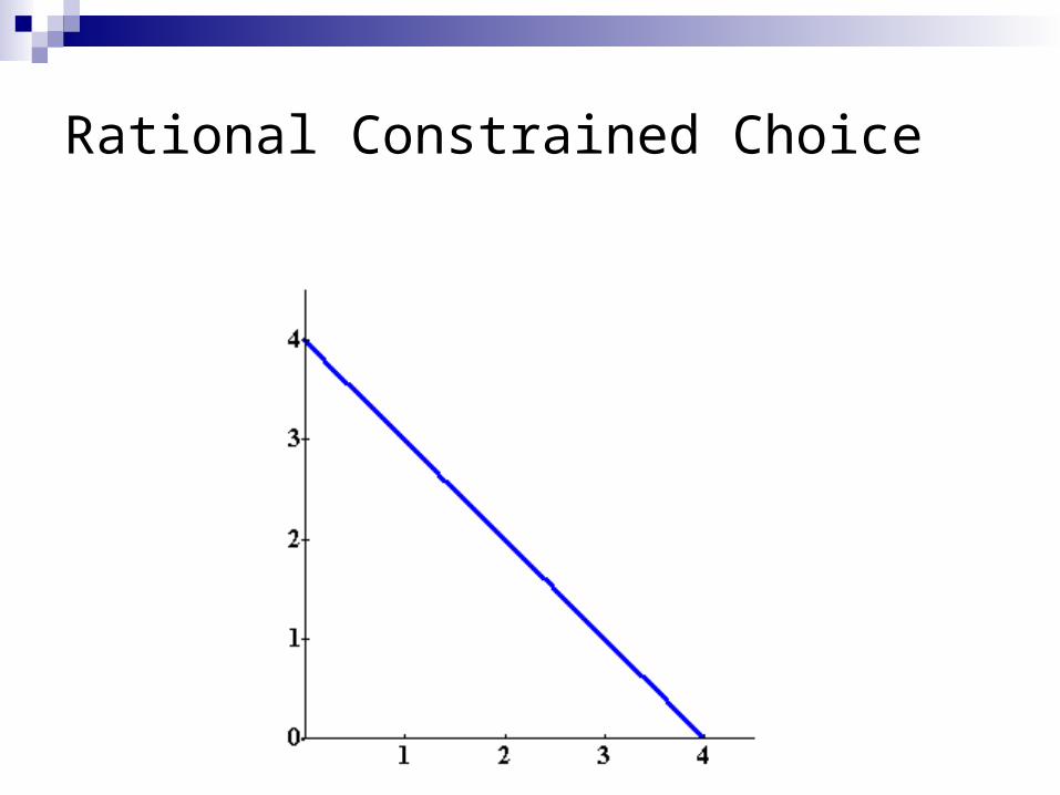
We’ve got budgets, we’ve got preferences What are people going to choose?

Behavioral Assumption: a decisionmaker chooses its most preferred alternative from those available to it.

The available choices constitute the choice set. How is the most preferred bundle in the choice

set located?

3

Rational Constrained Choice

x1

x2

4x1

x2


5x1

x2

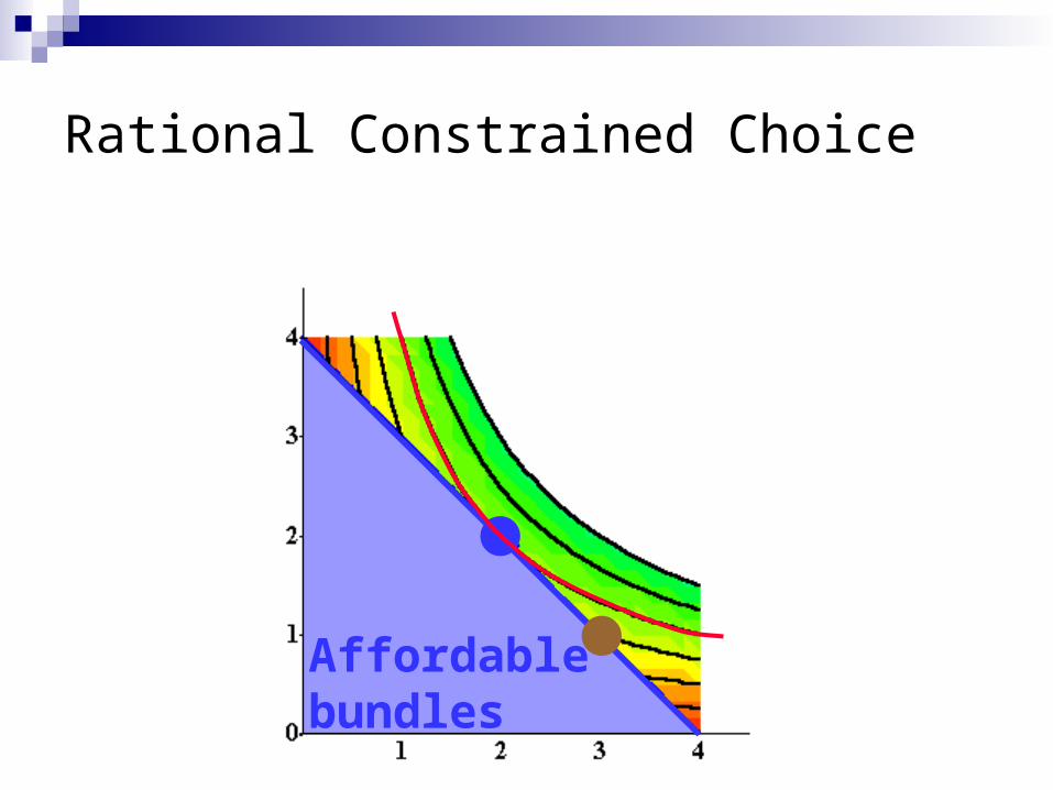
Affordablebundles


6x1

x2

Affordablebundles


7x1

x2

Affordablebundles

More preferredbundles


8

Affordablebundles

x1

x2

More preferredbundles


9

x1

x2

x1*

x2*

(x1*,x2*) is the mostpreferred affordablebundle.


10

The most preferred affordable bundle is called the consumer’s ordinary demand at the given prices and budget.

Ordinary demands will be denoted byx1*(p1,p2,m) and x2*(p1,p2,m).


11

When x1* > 0 and x2* > 0 the demanded bundle is interior.

If buying (x1*,x2*) costs $m then the budget is exhausted.


12

x1

x2

x1*

x2*

(x1*,x2*) is interior.(a) (x1*,x2*) exhausts thebudget: p1x1* + p2x2* = m.


13

x1

x2

x1*

x2*

(x1*,x2*) is interior .(b) The slope of the indiff.curve at (x1*,x2*) equals the slope of the budget constraint.


14

(x1*,x2*) satisfies two conditions: (a) the budget is exhausted

p1x1* + p2x2* = m (b) the slope of the budget constraint,

-p1/p2, and the slope of the indifference curve containing (x1*,x2*) are equal at (x1*,x2*).


15

Computing Ordinary Demands

How can this information be used to locate (x1*,x2*) for given p1, p2 and m?

16

Computing Ordinary Demands - a Cobb-Douglas Example.

Suppose that the consumer has Cobb-Douglas preferences.

U x x x xa b( , )1 2 1 2

17

Suppose that the consumer has Cobb-Douglas preferences.

Then

U x x x xa b( , )1 2 1 2

MUUx

ax xa b1

1112

MUUx

bx xa b2

21 2

1


18

So the MRS is

At (x1*,x2*), MRS = -p1/p2 so

MRSdxdx

U xU x

ax x

bx x

axbx

a b

a b

2

1

1

2

112

1 21

2

1

//

.

ax

bx

pp

xbpap

x2

1

1

22

1

21

*

** *. (A)


19

(x1*,x2*) also exhausts the budget so

p x p x m1 1 2 2* * . (B)


20

So now we know thatx

bpap

x21

21

* * (A)

p x p x m1 1 2 2* * . (B)


21

So now we know thatx

bpap

x21

21

* * (A)

p x p x m1 1 2 2* * . (B)

p x pbpap

x m1 1 21

21

* * .

Substitute

and get

This simplifies to ….


22

xam

a b p11

*

( ).


23

xbm

a b p22

*

( ).

Substituting for x1* in p x p x m1 1 2 2

* *

then gives

xam

a b p11

*

( ).


24

So we have discovered that the mostpreferred affordable bundle for a consumerwith Cobb-Douglas preferences

U x x x xa b( , )1 2 1 2

is( , )

( ),( )

.* * ( )x xam

a b pbm

a b p1 21 2


25


x1

x2

xam

a b p11

*

( )

x

bma b p

2

2

*

( )

U x x x xa b( , )1 2 1 2

26


When x1* > 0 and x2* > 0 and (x1*,x2*) exhausts the budget, and indifference curves have no ‘kinks’, the ordinary demands are obtained by solving:

(a) p1x1* + p2x2* = m (b) the slopes of the budget constraint, -

p1/p2, and of the indifference curve containing (x1*,x2*) are equal at (x1*,x2*).

27


But what if x1* = 0?

Or if x2* = 0?

If either x1* = 0 or x2* = 0 then the ordinary demand (x1*,x2*) is at a corner solution to the problem of maximizing utility subject to a budget constraint.

28

Examples of Corner Solutions -- the Perfect Substitutes Case

x1

x2

MRS = -1

29

x1

x2

MRS = -1

Slope = -p1/p2 with p1 > p2.


30

x1

x2

xy

p22

*

x1 0*

MRS = -1

Slope = -p1/p2 with p1 > p2.


31

x1

x2

xyp11

*

x2 0*

MRS = -1

Slope = -p1/p2 with p1 < p2.


32

So when U(x1,x2) = x1 + x2, the mostpreferred affordable bundle is (x1*,x2*)where

0,py

)x,x(1

*2

*1

and

2

*2

*1 p

y,0)x,x(

if p1 < p2

if p1 > p2.


33

x1

x2

MRS = -1

Slope = -p1/p2 with p1 = p2.

yp1

yp2


34

x1

x2

All the bundles in the constraint are equally the most preferred affordable when p1 = p2.

yp2

yp1


35

Examples of ‘Kinky’ Solutions -- the Perfect Complements Case

x1

x2U(x1,x2) = min{ax1,x2}

x2 = ax1

36

x1

x2

MRS = -

MRS = 0

MRS is undefined

U(x1,x2) = min{ax1,x2}

x2 = ax1


37

x1


x2 = ax1

Which is the mostpreferred affordable bundle?


38

x1


x2 = ax1

The most preferredaffordable bundle


39

x1


x2 = ax1

x1*

x2*

(a) p1x1* + p2x2* = m(b) x2* = ax1*


40

(a) p1x1* + p2x2* = m; (b) x2* = ax1*.


41

(a) p1x1* + p2x2* = m; (b) x2* = ax1*.

Substitution from (b) for x2* in (a) gives p1x1* + p2ax1* = m


42

(a) p1x1* + p2x2* = m; (b) x2* = ax1*.

Substitution from (b) for x2* in (a) gives p1x1* + p2ax1* = mwhich gives

21

*1 app

mx


43

(a) p1x1* + p2x2* = m; (b) x2* = ax1*.

Substitution from (b) for x2* in (a) gives p1x1* + p2ax1* = mwhich gives .

appam

x;app

mx

21

*2

21

*1


44

x1


x2 = ax1

xm

p ap11 2

*

x

amp ap

2

1 2

*


choice

Documents

ordinary demand x1

cobbdouglas example

thencomputing ordinary

rational constrained

rational constrained

computing ordinary demandshow

budget constraint

consumers ordinary demand