cholesky and ldlt decomposition - mathematics for...

04.11.1

Chapter 04.11 Cholesky and LDLT Decomposition After reading this chapter, you should be able to:

1. understand why the LDLT algorithm is more general than the Cholesky algorithm, 2. understand the differences between the factorization phase and forward solution

phase in the Cholesky and LDLT algorithms, 3. find the factorized [L] and [D] matrices, 4. obtain the forward solution phase, 5. obtain the diagonal scaling phase, 6. obtain the backward solution phase, 7. solve a set of simultaneous linear equations using LDLT algorithm.

Introduction Solving large (and sparse) system of simultaneous linear equations (SLE) has been (and continues to be) a major challenging problem for many real-world engineering/science applications [1-2]. In matrix notation, at set of SLE can be represented as:

][]][[ bxA = (1) where

][A = known coefficient matrix, with dimension nn× ][b = known right-hand-side (RHS) 1×n vector ][x = unknown 1×n vector.

Symmetrical Positive Definite (SPD) SLE

For many practical SLE, the coefficient matrix ][A (see Equation (1)) is Symmetric Positive Definite (SPD). In this case, the efficient a 3-step Cholesky algorithm [1-2] can be used. A symmetric matrix nnA ×][ is SPD if either of the following conditions is satisfied:

(a) If each and every determinant of sub-matrix ),...,2,1( niAii = is positive, or..

(b) If 0>AyyT for any given vector 0][ 1

≠×ny

04.11.2 Chapter 04.11 Example 1 Find if

−−−

−=

110121

012][A

is SPD? Solution

Criterion a: If each and every determinant of sub-matrix ),...,2,1( niAii = is positive. The given 33× matrix ][A is symmetrical, because jiij aa = . Furthermore, one has

[ ] 022det 11 >==×A

[ ]

032112

det 22

>=

−−

=×A

[ ]

01110121

012det 33

>=

−−−

−=×A

Hence ][A is SPD. Criterion (b): If 0>AyyT for any given vector 0][ 1

≠×ny For any given vector

0

3

2

1

≠

=

yyy

y ,

one computes

[ ]

( ) { }( ) { }32

23

22

21

221

3223

2221

21

3

2

1

321

2

2222

110121

012

yyyyyyy

yyyyyyy

yyy

yyyAyyT

−+++−=

−++−=

−−−

−=

( ) ( ) 0232

21

221 >−++−= yyyyy

Since the above scalar is always positive, hence matrix ][A is SPD.

Cholesky and LDLT Decomposition 04.11.3 Step 1: Matrix Factorization phase

In this step, the coefficient matrix ][A that is SPD can be decomposed (or factorized) into ][][][ UUA T= (2)

where, ][U is a nn× upper triangular matrix.

The following simple 33× matrix example will illustrate how to find the matrix ][U . Various terms of the factorized matrix ][U can be computed/derived as follows (see Equation (2)):

=

33

2322

131211

332313

2212

11

333231

232221

131211

0000

00

uuuuuu

uuuuu

u

aaaaaaaaa

(3)

Multiplying two matrices on the right-hand-side (RHS) of Equation (3), and then equating each upper-triangular RHS terms to the corresponding ones on the upper-triangular left-hand-side (LHS), one gets the following 6 equations for the 6 unknowns in the factorized matrix

][U .

1111 au = ;11

1212 u

au = ;

11

1313 u

au = (4)

( )21

2122222 uau −= ;

22

13122323 u

uuau

−= ; ( )2

1223

2133333 uuau −−= (5)

In general, for a nn× matrix, the diagonal and off-diagonal terms of the factorized matrix ][U can be computed from the following formulas:

( )21

1

1

2

−= ∑

−

=

i

kkiiiii uau (6)

ii

i

kkjkiij

ij u

uuau

∑−

=

−=

1

1 (7)

It is noted that if ji = , then the numerator of Equation (7) becomes identical to the terms under the square root in Equation (6). In other words, to factorize a general term iju , one simply needs to do the following steps: Step 1.1: Compute the numerator of Equation (7), such as

∑−

=

−=1

1

i

kkjkiij uuaSum

Step 1.2 If iju is an off-diagonal term (say, ji < ) then from Equation (7)

iiij u

Sumu =

else, if iju is a diagonal term (that is, ji = ), then from Equation (6)

04.11.4 Chapter 04.11

Sumuii = As a quick example, one computes:

55

47453735272517155757 u

uuuuuuuuau

−−−−= (8)

Thus, for computing )7,5( == jiu , one only needs to use the (already factorized) data in columns )5(# =i , and )7(# =j of ][U , respectively.

In general, to find the (off-diagonal) factorized term iju , one only needs to utilize the “already factorized” columns i# , and j# information (see Figure 1). For example, if 5=i , and 7=j , then Figure 1 will lead to the same formula as shown earlier in Equation (7), or in Equation (8). Similarly, to find the (diagonal) factorized term iiu , one simply needs to utilize columns i# , and i# (again!) information (see Figure 1). In this case, Figure 1 will lead to the same formula as shown earlier in Equation (6).

k = 1

k = 2

k = 3

k = 4

iiu iju

ju4

ju3

ju2

ju1

iu4

iu3

iu2

iiu

i = 5

Col. # i=5 Col. # j=7

Figure 1 Cholesky Factorization for the term iju

Since the square root operation involved during the Cholesky factorization phase (see Equation (6)), one must make sure the term under the square root is non-negative. This requirement satisfied by ][A being SPD. Step 2: Forward Solution phase Substituting Equation (2) into Equation (1), one gets

][]][[][ bxUU T = (9) Let us define

][][][ yxU ≡ (10) Then, Equation (9) becomes

][][][ byU T = (11) Since TU ][ is a lower triangular matrix, Equation (11) can be efficiently solved for the intermediate unknown vector ][y , according to the order

Cholesky and LDLT Decomposition 04.11.5

ny

yy

.

.2

1

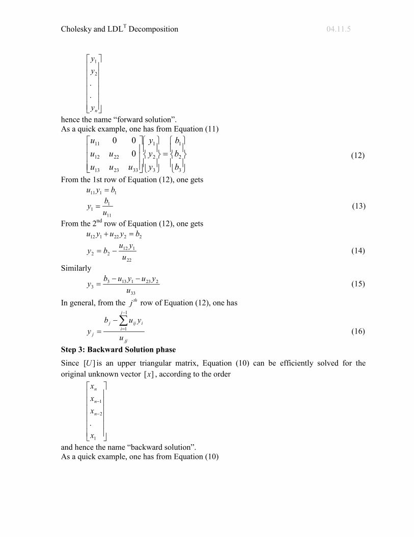
hence the name “forward solution”. As a quick example, one has from Equation (11)

=

3

2

1

3

2

1

332313

2212

11

000

bbb

yyy

uuuuu

u

(12)

From the 1st row of Equation (12), one gets 1111 byu =

11

11 u

by = (13)

From the 2nd row of Equation (12), one gets 2222112 byuyu =+

22

11222 u

yuby −= (14)

Similarly

33

22311333 u

yuyuby −−= (15)

In general, from the thj row of Equation (12), one has

jj

j

iiijj

j u

yuby

∑−

=

−=

1

1 (16)

Step 3: Backward Solution phase

Since ][U is an upper triangular matrix, Equation (10) can be efficiently solved for the original unknown vector ][x , according to the order

−

−

1

2

1

.x

xxx

n

n

n

and hence the name “backward solution”. As a quick example, one has from Equation (10)

04.11.6 Chapter 04.11

=

3

2

1

3

2

1

33

2322

131211

000

yyy

xxx

uuuuuu

(17)

From the last (or rdthn 3= ) row of Equation (17), one has 3333 yxu = .

hence

33

33 u

yx = (18)

Similarly

22

32322 u

xuyx

−= (19)

and

11

31321211 u

xuxuyx

−−= (20)

In general, one has

jj

n

jiijij

j u

xuyx

∑+=

−= 1 (21)

Amongst the above 3-step Cholesky algorithms, factorization phase in step 1 consumes about 95% of the total SLE solution time.

If the coefficient matrix ][A is symmetrical but not necessarily positive definite, then the above Cholesky algorithms will not be valid. In this case, the following TLDL factorized algorithms can be employed

TLDLA ]][][[][ = (22) For example

=

10010

1

000000

101001

32

3121

33

22

11

3231

21

333231

232221

131211

lll

dd

d

lll

aaaaaaaaa

(23)

Multiplying the three matrices on the RHS of Equation (23), then equating the resulting upper-triangular RHS terms of Equation (23) to the corresponding ones on the LHS, one obtains the following formulas for the diagonal ][D , and lower-triangular ][L matrices

∑−

=

−=1

1

2j

kkkjkjjjj dlad (24)

×

−= ∑

−

= jj

j

kjkkkikijij d

ldlal 11

1

(25)

Thus, the TLDL algorithms can be summarized by the following step-by-step procedures.

Cholesky and LDLT Decomposition 04.11.7 Step1: Factorization phase

TLDLA ]][][[][ = (22, repeated) Step 2: Forward solution and diagonal scaling phase Substituting Equation (22) into Equation (1), one gets

][][]][][[ bxLDL T = (26) Let us define

][][][ yxL T =

=

3

2

1

3

2

1

32

3121

10010

1

yyy

xxx

lll

(27)

1,2,...,1,;1

−=−= ∑+=

nniforxlyxn

ikkkiii (28)

Also, define ][]][[ zyD =

=

3

2

1

3

2

1

33

22

11

000000

zzz

yyy

dd

d (29)

nifordzy

ii

ii ......,,3,2,1, == (30)

Then Equation (26) becomes ][]][[ bzL =

=

3

2

1

3

2

1

3231

21

101001

bbb

zzz

lll (31)

niforzLbzi

kkikii ......,,3,2,1

1

1=−= ∑

−

=

(32)

Equation (31) can be efficiently solved for the vector [ ]z , and then Equation (29) can be conveniently (and trivially) solved for the vector [ ]y . Step 3: Backward solution phase

In this step, Equation (27) can be efficiently solved for the original unknown vector [ ]x . Example 2

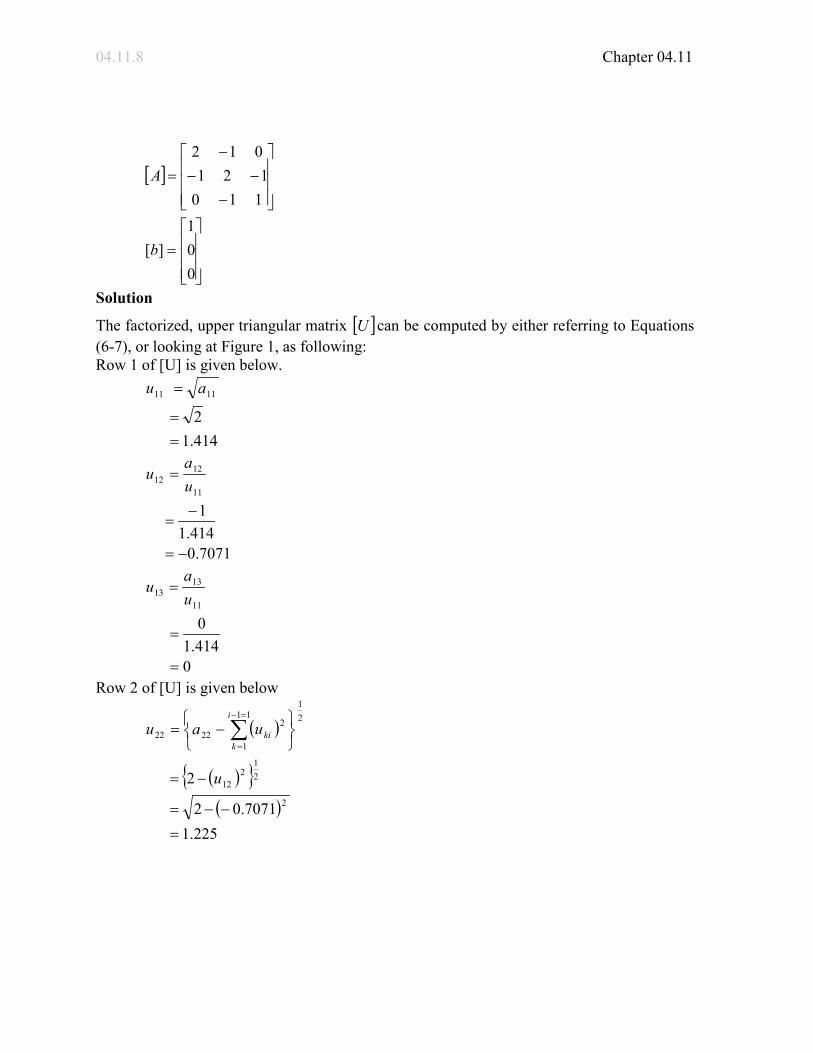
Using the Cholesky algorithm, solve the following SLE system for the unknown vector [ ]x . ][]][[ bxA =

where

04.11.8 Chapter 04.11

[ ]

−−−

−=

110121

012A

=

001

][b

Solution

The factorized, upper triangular matrix [ ]U can be computed by either referring to Equations (6-7), or looking at Figure 1, as following: Row 1 of [U] is given below.

414.12

1111

==

= au

7071.0414.1

111

1212

−=

−=

=ua

u

0414.10

11

1313

=

=

=ua

u

Row 2 of [U] is given below

( )

( ){ }( )

225.17071.02

22

21

212

21

11

1

22222

=

−−=

−=

−= ∑=−

=

u

uaui

kki


( )( )

8165.0225.1

07071.01225.1

1 1312

22

11

123

23

−=

−−−=

×−−=

−=

∑=−

=

uuU

uuau

i

kkjki

Row 3 of [U] is given below

( )

{ }( ) ( )

5774.08165.001 22

21

223

21333

21

21

1

23333

=

−−−=

−−=

−= ∑=−

=

uua

uaui

kki

Thus, the factorized matrix

[ ]

−

−=

5774.0008165.0225.1007071.0414.1

U

The forward solution phase, shown in Equation (11), becomes [ ] [ ] [ ]byU T =

=

−−

001

5774.08165.000225.17071.000414.1

3

2

1

yyy

Thus, Equation (16) can be used to solve for [y] as

7071.0414.11

11

11

=

=

=uby

( )( )( )

4082.0225.1

7071.07071.00

22

112

11

12

2

==

=−=−=

−=

∑=−

=

uyu

u

yuby

jj

j

iiij

04.11.10 Chapter 04.11

( )( ) ( )( )( )

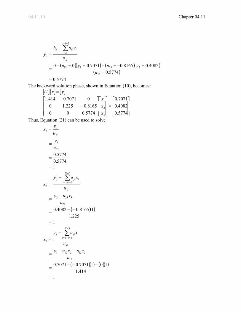
5774.05774.0

4082.08165.07071.000

33

223113

21

13

3

==

=−=−==−=

−=

∑=−

=

uyuyu

u

yuby

jj

j

iiij

The backward solution phase, shown in Equation (10), becomes: [ ] [ ] [ ]yxU =

=

−

−

5774.04082.07071.0

5774.0008165.0225.1007071.0414.1

3

2

1

xxx

Thus, Equation (21) can be used to solve

15774.05774.0

33

3

3

=

=

=

=

uy

uy

xjj

j

( )( )

1225.1

18165.04082.022

3232

3

312

=

−−=

−=

−=

∑=

=+=

uxuy

u

xuyx

jj

N

jiijij

( )( ) ( )( )

1414.1

1017071.07071.011

3132121

3

211

=

−−−=

−−=

−=

∑=

=+=

uxuxuy

u

xuyx

jj

N

jiijij

Cholesky and LDLT Decomposition 04.11.11 Hence

=

111

][x

Example 3

Using the LDLT algorithm, solve the following SLE system for the unknown vector [ ]x . ][]][[ bxA =

where

[ ]

−−−

−=

110121

012A

=

001

][b

Solution

The factorized matrices ][D and ][L can be computed from Equation (24) and Equation (25), respectively.

[ ] [ ]LandDofmatricesofColumn

da

l

da

d

ldlal

alwaysl

a

dlad

jj

j

kjkkkik

j

kkkjk

1

020

5.021

)!(12

11

3131

11

21

01

121

21

11

11

01

1

21111

=

=

=

−=

−=

=

−=

===

−=

∑

∑

=−

=

=−

=

04.11.12 Chapter 04.11

( ) ( )

( )( )( )

[ ] [ ]LandDmatricesofColumn

d

ldlal

alwaysl

dl

dlad

j

k

j

kkkjk

2

6667.05.1

5.0201

)!(15.1

25.02

2

22

11

121113132

32

22

211

221

11

1

22222

−=

−−−=

−=

==

−−=

−=

−=

∑

∑

=−

=

=−

=

( ) ( ) ( ) ( )[ ] [ ]LandDmatricesofColumndldl

dladj

kkkjk

3

3333.05.16667.0201

122

2223211

231

21

1

23333

=−−−=

−−=

−= ∑=−

=

Hence

[ ]

=

3333.00005.10002

D

and

[ ]

−−=

16667.00015.0001

L

The forward solution shown in Equation (31) becomes: [ ] [ ] [ ]bzL =

=

−−

001

1667.00015.0001

3

2

1

zzz

, or

∑−

=

−=1

1

i

kkikii zlbz (32, repeated)

Hence


( )( )

( )( ) ( )( )3333.0

5.06667.0100

5.015.00

1

23213133

12122

11

=−−−=

−−==

−−=−===

zLzLbz

zLbzbz

The diagonal scaling phase, shown in Equation (29) becomes [ ] [ ] [ ]zyD =

=

3333.05.0

1

3333.00005.10002

3

2

1

yyy

, or

ii

ii d

zy =

Hence

5.021

11

11

=

=

=dzy

3333.05.15.022

22

=

=

=dzy

13333.03333.033

33

=

=

=dzy

The backward solution phase can be found by referring to Equation (27) [ ] [ ] [ ]yxL T =

=

−

−

1333.05.0

100667.01005.01

3

2

1

xxx

∑+=

−=N

ikkkiii xlyx

1

(28, repeated)

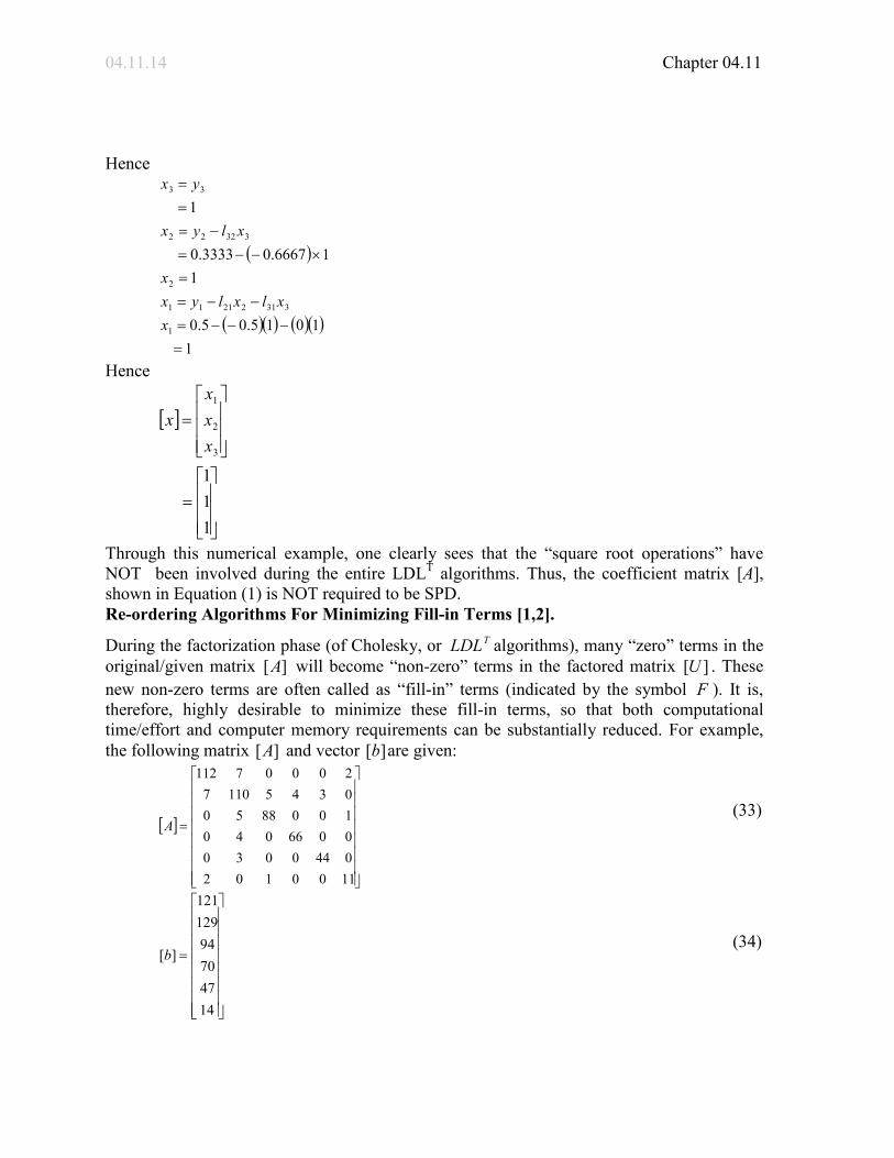
04.11.14 Chapter 04.11 Hence

( )

( )( ) ( )( )1

1015.05.0

116667.03333.0

1

1

33122111

2

33222

33

=−−−=

−−==

×−−=−=

==

xxlxlyx

x

xlyx

yx

Hence

[ ]

=

=

111

3

2

1

xxx

x

Through this numerical example, one clearly sees that the “square root operations” have NOT been involved during the entire LDLT algorithms. Thus, the coefficient matrix [A], shown in Equation (1) is NOT required to be SPD. Re-ordering Algorithms For Minimizing Fill-in Terms [1,2].

During the factorization phase (of Cholesky, or TLDL algorithms), many “zero” terms in the original/given matrix ][A will become “non-zero” terms in the factored matrix ][U . These new non-zero terms are often called as “fill-in” terms (indicated by the symbol F ). It is, therefore, highly desirable to minimize these fill-in terms, so that both computational time/effort and computer memory requirements can be substantially reduced. For example, the following matrix ][A and vector ][b are given:

[ ]

=

11001020440030006604010088500345110720007112

A (33)

=

14477094

129121

][b (34)

Cholesky and LDLT Decomposition 04.11.15 The Cholesky factorization matrix ][U , based on the original matrix ][A (see Equation 33) and Equations (6-7), or Figure 1, can be symbolically computed as

[ ]

××

×××

×××××××

=

000000000

00000

0000

FFF

FFF

U (35)

In Equation (35), the symbols x , and F represents the “non-zero” and “fill-in” terms, respectively.

In practical applications, however, it is always a necessary step to rearrange the original matrix ][A through re-ordering algorithms (or subroutines) [Refs 1-2] and produce the following integer mapping array

IPERM (new equation #) = {old equation #} (36) such as, for this particular example:

=

123456

654321

IPERM (37)

Using the above results (see Equation 37), one will be able to construct the following re-arranged matrices:

[ ]

=

11270002711054300588001040660003004402010011

*A (38)

and

=

12112994704714

][ *b (39)

In the original matrix A (shown in Equation 33), the nonzero term A (old row 1, old column 2) = 7 will move to new location *A of the new matrix (new row 6, new column 5

The non zero term

) = 7, etc.

A (old row 3, old column 3) = 88 will move to *A (new row 4, new column 4) = 88, etc.

The value of b (old row 4) = 70 will be moved to (or located at) *b (new row 3) = 70, etc.

04.11.16 Chapter 04.11

Now, one would like to solve the following modified system of linear equations (SLE) for ][ *x ,

][]][[ *** bxA = (40) rather than to solve the original SLE (see Equation (1)). The original unknown vector }{x can

be easily recovered from ][ *x and [ ]IPERM , shown in Equation (37). The factorized matrix ][ *U can be “symbolically” computed from ][ *A as (by referring to either Figure 1 or Equations 6-7):

[ ]

×××

××××××

×××

=

000000000

00000000000

000

*

FU

(41)

You can clearly see the big benefits of solving the SLE shown in Equation (40), instead of solving the original Equation (1), since the factorized matrix ][ *U has only 1 fill-in term (see the symbol “ F ” in Equation 41), as compared to six fill-in-terms occurred in the factorized matrix ][U as shown in Equation 35. On-Line Chess-Like Game For Reordering/Factorized Phase [4]. Based on the discussions presented in the previous section 2 (about factorization phase), and section 3 (about reordering phase), one can easily see the similar operations between the symbolic, numerical factorization and reordering (to minimize the number of fill-in terms) phases of sparse SLE.

In practical computer implementation for the solution of SLE, the reordering phase is usually conducted first (to produce the mapping between “old↔new” equation numbers, as indicated in the integer array IPERM(-), see Equations 36-37).

Then, the sparse symbolic factorization phase is followed by using either Cholesky Equations 6-7, or the TLDL Equations 24-25 (without requiring the actual/numerical values to be computed). The reason is because during the symbolic factorization phase, one only wishes to find the number (and the location) of non-zero fill-in terms. This symbolic factorization process is necessary for allocating the “computer memory” requirement for the “numerical factorization” phase which will actually compute the exact numerical values of

][ *U , based on the same Cholesky Equations (6-7) (or the TLDL Equations (24-25)). In this work, a chess-like game (shown in Figure 2, Ref. [4]) has been designed with

the following objectives:


Figure 2 A Chess-Like Game For Learning to Solve SLE.

(A) Teaching undergraduates the process how to use the reordering output IPERM(-), see Equations (36-37) for converting the original/given matrix ][A , see Equation (33), into the new/modified matrix ][ *A , see Equation (38). This step is reflected in Figure 2, when the “Game Player” decides to swap node (or equation) i (say 2=i ) with another node (or equation) j, and click the CONFIRM icon! Since node i=2 is currently connected to nodes j =4, 6, 7, 8, swapping node 2=i with the above nodes j will NOT change the number/pattern of the fill-in terms. However, if node

2=i is swapped with node j=1, or 3 or 5, then the fill-in terms pattern may change (for better or worse)!

(B) Helping undergraduates to understand the “symbolic” factorization” phase by symbolically utilizing the Cholesky factorized Equations (6-7). This step is illustrated in Figure 2, for which the “game player” will see (and also hear the computer animated sound, and human voice) the non-zero terms (including fill-in terms) of the original matrix ][A to move to the new locations in the new/modified matrix ][ *A .

(C) Helping undergraduates to understand the numerical factorization phase, by numerically utilizing the same Cholesky factorized Equations (6-7).

(D) Teaching undergraduates to understand existing reordering concepts, or to discover new reordering algorithms.

Further Explanation on the Developed Game

1. In the above chess-like game, which is available on-line [4], powerful features of FLASH computer environment [3], such as animated sound, human voice, motions, graphical colors etc… have been incorporated and programmed into the developed game-software for more appeal to game players/learners.

2. In the developed chess-like game, fictitious monetary (or any kind of ‘scoring system”) is rewarded (and broadcasted by computer animated human voice) to game players, based on how he/she swaps the node (or equation) numbers, and consequently based on how many fill-in F terms occurred. In general, less fill-in terms introduced will result in more rewards.

3. Based on the original/given matrix ][A , and existing re-ordering algorithms (such as the Reverse Cuthill-Mckee, or RCM algorithms [1-2]) the number of fill-in terms F can be computed using RCM algorithms. This internally generated information will be used to judge how good the players/learners are, and/or broadcast “congratulations

04.11.18 Chapter 04.11

message” to a particular player who discovers a new “chess-like move” (or, swapping node) strategies which are even better than RCM algorithms.

4. Initially, the player(s) will select the matrix size ( 88× , or larger is recommended), and the percentage (50%, or larger is suggested) of zero-terms (or sparsity of the matrix). Then, the START Game icon will be clicked by the player.

5. The player will then CLICK one of the selected node i (or equation) numbers appearing on the computer screen. The player will see those nodes j which are connected to node i (based on the given/generated matrix ][A ). The player then has to decide to swap node i with one of the possible node j . After confirming the player’s decision, the outcomes/results will be announced by the computer animated human voice, and the monetary-award will (or will not) be given to the players/learners, accordingly. In this software, a maximum of $1,000,000 can be earned by the player, and the exact dollar amount will be inversely proportional to the number of fill-in terms occurred (based on the player’s decision on how to swap node i with another node j ).

6. The next player will continue to play, with his/her move (meaning to swap the thi node with the thj node) based on the current best non-zero terms pattern of the matrix.

References

CHOLSEKY AND LDLT DECOMPOSITION Topic Cholesky and LDLT Decomposition Summary Textbook chapter of Cholesky and LDLT Decomposition Major General Engineering Authors Duc Nguyen Date July 29, 2010 Web Site http://numericalmethods.eng.usf.edu

cholesky and ldlt decomposition - mathematics for...

Documents