Shot-geophone migration for seismic data

Chris Stolk

Department of Applied Mathematics, University of Twente, The

Netherlands

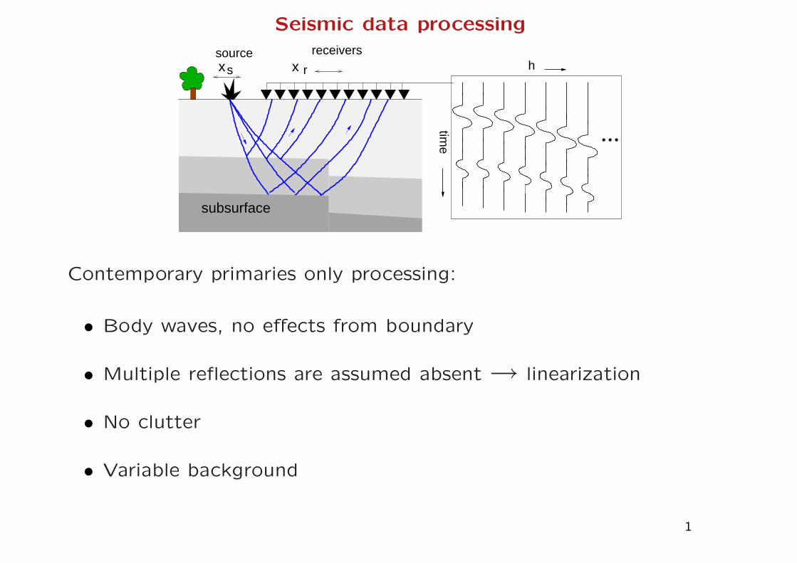
Seismic data processing

...time

hsource receivers

sx x r

subsurface

Contemporary primaries only processing:

• Body waves, no effects from boundary

• Multiple reflections are assumed absent→ linearization

• No clutter

• Variable background

1

Outline

Part I Imaging in a smoothly varying background

– Phase space (microlocal) point of view

– Geometry of scattering

– Minimal data (dimension n) / maximal data (dimension 2n−1)

Part II Constructing multiple images for velocity estimation

2

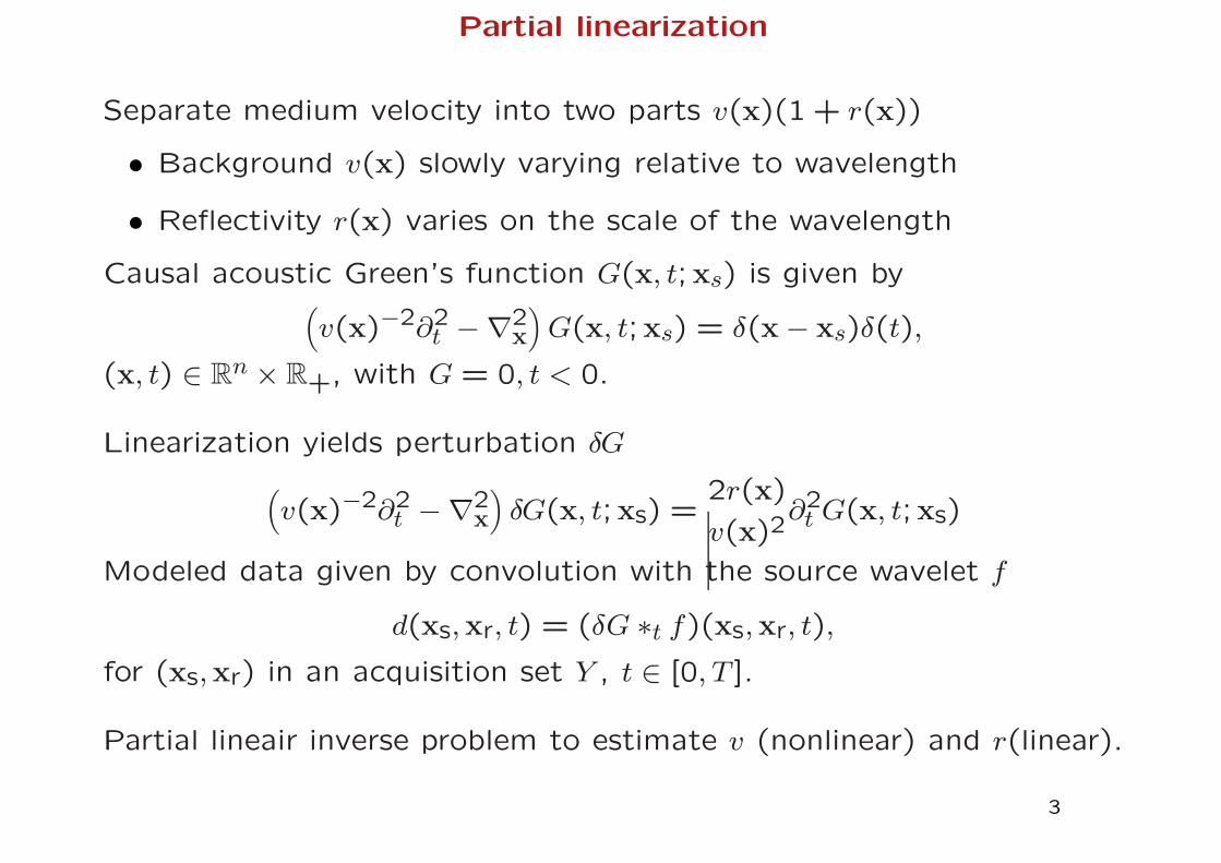
Partial linearization

Separate medium velocity into two parts v(x)(1 + r(x))

• Background v(x) slowly varying relative to wavelength

• Reflectivity r(x) varies on the scale of the wavelength

Causal acoustic Green’s function G(x, t;xs) is given by(

v(x)−2∂2t −∇

2x

)

G(x, t;xs) = δ(x− xs)δ(t),

(x, t) ∈ Rn × R+, with G = 0, t < 0.

Linearization yields perturbation δG

(

v(x)−2∂2t −∇

2x

)

δG(x, t;xs) =2r(x)

v(x)2∂2

t G(x, t;xs)

Modeled data given by convolution with the source wavelet f

d(xs,xr, t) = (δG ∗t f)(xs,xr, t),

for (xs,xr) in an acquisition set Y , t ∈ [0, T ].

Partial lineair inverse problem to estimate v (nonlinear) and r(linear).

3

Geometrical wave propagation

Simultaneous localization in position and wave vector space (phase

space). Consider e.g. a sizeable Fourier coefficient of a plane wave

component

eiω(p·x−t)

even after muting signal outside a neighborhood of some point (x, t0).

Solutions of the wave equation have the property that high-frequency

local plane wave components approximately propagate along a ray

t 7→ (X(t), P(t)), with X(t0) = x, P(t0) = p,

given by an ODE, if p and P(t) satisfy the dispersion relation ‖p‖ =

v(x)−1.

In ray theory one can distinguish between

• Rays, traveltimes (kinematics) ← this talk

• Amplitudes (dynamics)

4

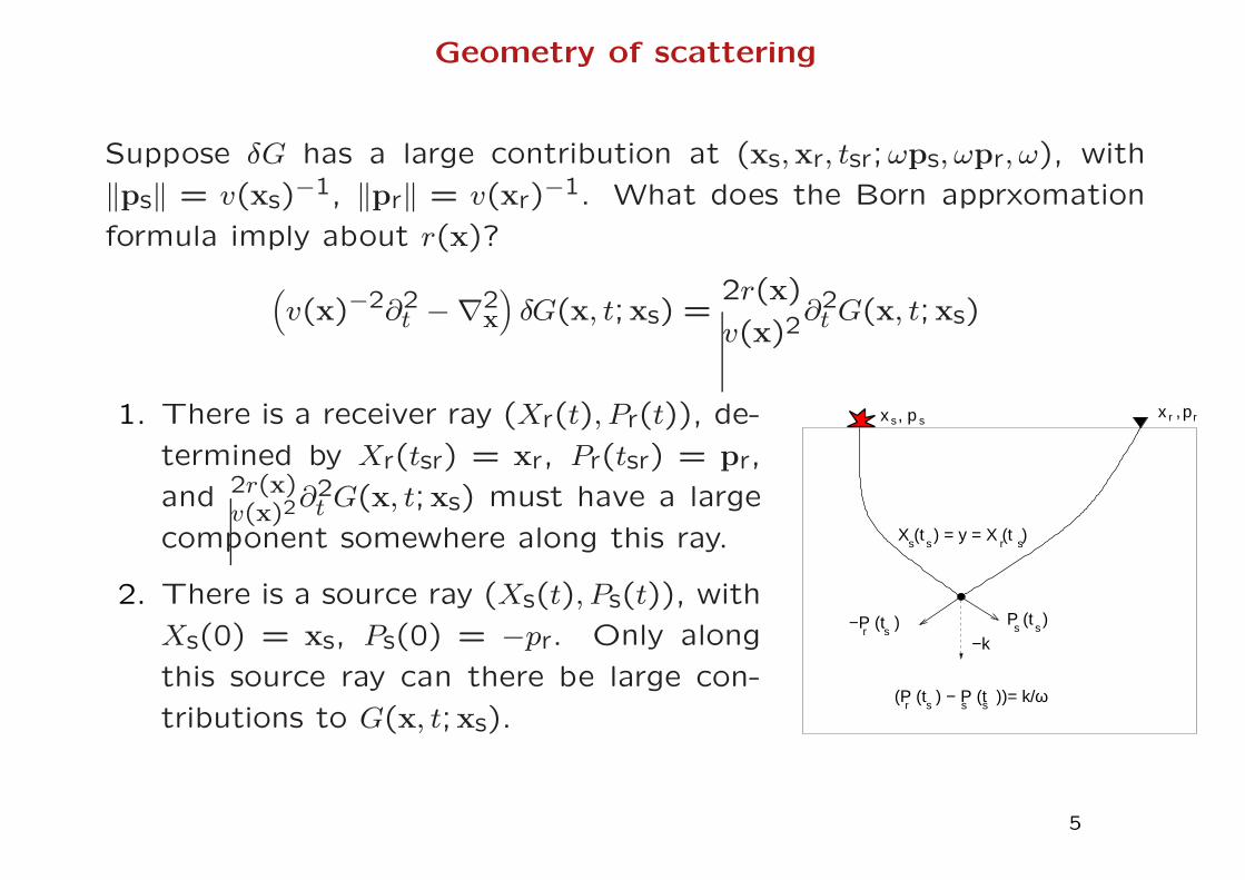
Geometry of scattering

Suppose δG has a large contribution at (xs,xr, tsr;ωps, ωpr, ω), with

‖ps‖ = v(xs)−1, ‖pr‖ = v(xr)−1. What does the Born apprxomation

formula imply about r(x)?

(

v(x)−2∂2t −∇

2x

)

δG(x, t;xs) =2r(x)

v(x)2∂2

t G(x, t;xs)

1. There is a receiver ray (Xr(t), Pr(t)), de-

termined by Xr(tsr) = xr, Pr(tsr) = pr,

and 2r(x)v(x)2

∂2t G(x, t;xs) must have a large

component somewhere along this ray.

r

s s

x sx ,

ssX (t ) = y = X (t )

r s(P (t ) − P (t ))= k/

P (t )r s

−P (t )

ω

, p s rp

sr

−k

s s

2. There is a source ray (Xs(t), Ps(t)), with

Xs(0) = xs, Ps(0) = −pr. Only along

this source ray can there be large con-

tributions to G(x, t;xs).

5

3. The rays must intersect at some y = Xs(ts) = Xr(ts), and 2r(x)v(x)2

must have a large contribution at (y;k) with

k = ω(Pr(ts)− Ps(ts))

around y. Snell’s law is satisfied because ‖Ps(ts)‖ = v(y)−1 =

‖Pr(ts)‖.

Relation (“scattering relation”) determined by the rays

(y, ω(Pr(ts)− Ps(ts))

coords. of energy in reflectivity↔ (xs,xr, tsr, ωps, ωpr, ω)

coords. of event in data

This is the canonical relation of the map F : r 7→ d as a Fourier

integral operator (Rakesh (1988), Ten Kroode et al. (1998)).

6

Restriction to the acquisition set

To localize an event in the data with respect to wave vector (ωps, ωpr),

sufficient sampling is required.

Assuming (xs,xr) densely sample a submanifold of Y of Rn−1×R

n−1,

then components of (ps,pr) normal to Y can not be obtained directly.

In case of maximal acquistion ((xs,xr) densely sampled along the

plane) the dispersion relation determines one component of ps and

similar for pr, and (ps,pr) is fully determined.

If Y is a lower dimensional submanifold of Rn−1 × Rn−1 then (ps,pr)

is not uniquely determined.

7

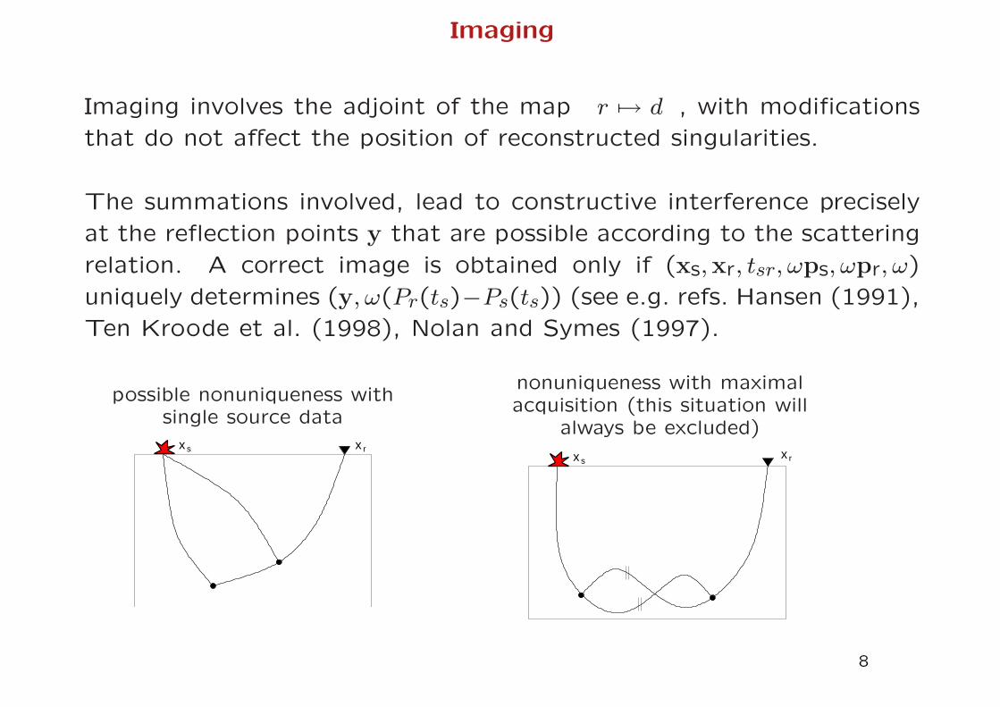
Imaging

Imaging involves the adjoint of the map r 7→ d , with modifications

that do not affect the position of reconstructed singularities.

The summations involved, lead to constructive interference precisely

at the reflection points y that are possible according to the scattering

relation. A correct image is obtained only if (xs,xr, tsr, ωps, ωpr, ω)

uniquely determines (y, ω(Pr(ts)−Ps(ts)) (see e.g. refs. Hansen (1991),

Ten Kroode et al. (1998), Nolan and Symes (1997).

possible nonuniqueness withsingle source data

rxx s

nonuniqueness with maximalacquisition (this situation will

always be excluded)

rx sx

8

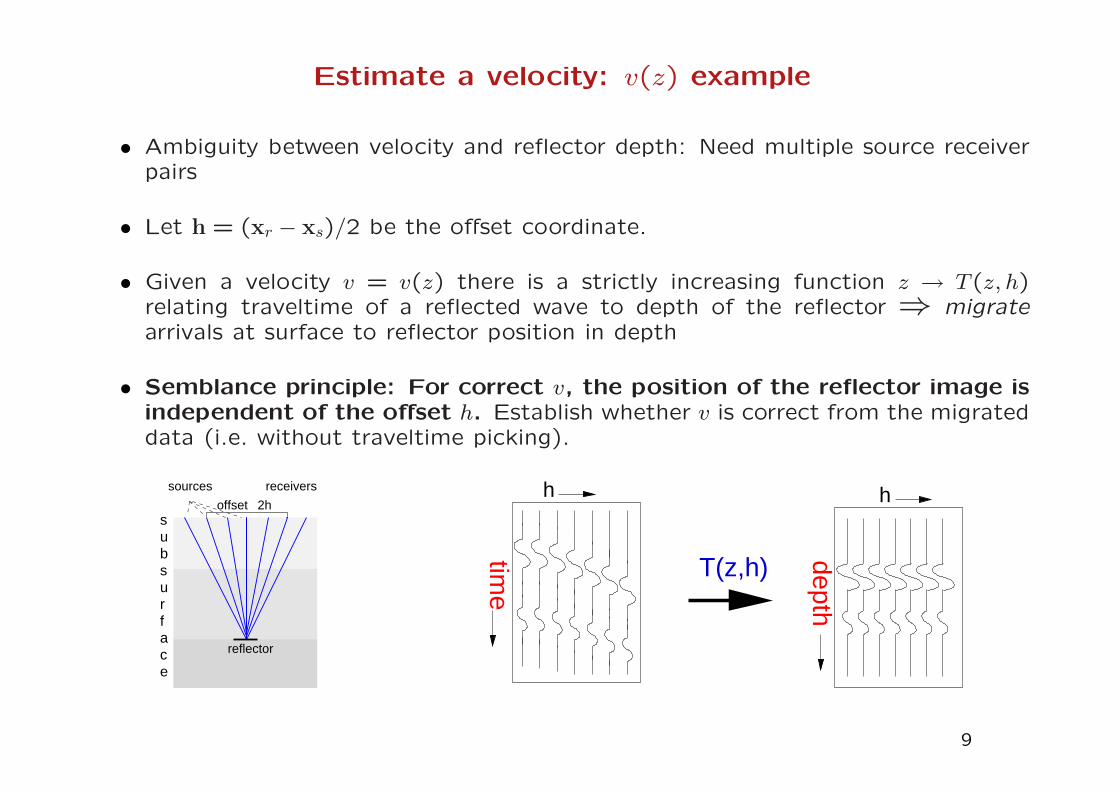
Estimate a velocity: v(z) example

• Ambiguity between velocity and reflector depth: Need multiple source receiverpairs

• Let h = (xr − xs)/2 be the offset coordinate.

• Given a velocity v = v(z) there is a strictly increasing function z → T(z, h)relating traveltime of a reflected wave to depth of the reflector ⇒ migrate

arrivals at surface to reflector position in depth

• Semblance principle: For correct v, the position of the reflector image isindependent of the offset h. Establish whether v is correct from the migrateddata (i.e. without traveltime picking).

subsurface

offset

reflector

receiverssources

2hh

time

h

depth

T(z,h)

9

Part II: Multiple images for velocity estimation

• General approach to derive prestack migration formulas

• Binning based migration schemes

• Shot-geophone migration

• Geometrical acoustics analysis of shot-geophone migration

• Examples

10

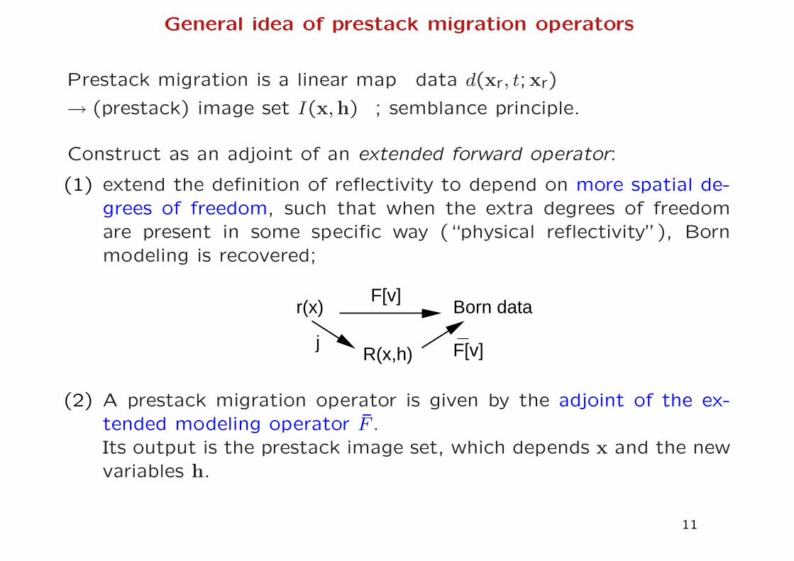
General idea of prestack migration operators

Prestack migration is a linear map data d(xr, t;xr)

→ (prestack) image set I(x, h) ; semblance principle.

Construct as an adjoint of an extended forward operator:

(1) extend the definition of reflectivity to depend on more spatial de-

grees of freedom, such that when the extra degrees of freedom

are present in some specific way (“physical reflectivity”), Born

modeling is recovered;

r(x)

R(x,h)

Born data

j

F[v]

F[v]

(2) A prestack migration operator is given by the adjoint of the ex-

tended modeling operator F .

Its output is the prestack image set, which depends x and the new

variables h.

11

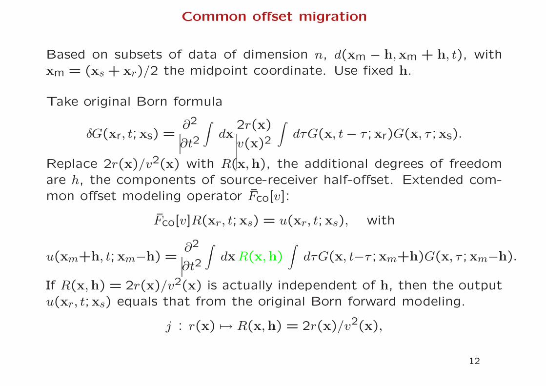
Common offset migration

Based on subsets of data of dimension n, d(xm − h,xm + h, t), with

xm = (xs + xr)/2 the midpoint coordinate. Use fixed h.

Take original Born formula

δG(xr, t;xs) =∂2

∂t2

∫

dx2r(x)

v(x)2

∫

dτG(x, t− τ ;xr)G(x, τ ;xs).

Replace 2r(x)/v2(x) with R(x, h), the additional degrees of freedom

are h, the components of source-receiver half-offset. Extended com-

mon offset modeling operator Fco[v]:

Fco[v]R(xr, t;xs) = u(xr, t;xs), with

u(xm+h, t;xm−h) =∂2

∂t2

∫

dxR(x, h)∫

dτG(x, t−τ ;xm+h)G(x, τ ;xm−h).

If R(x, h) = 2r(x)/v2(x) is actually independent of h, then the output

u(xr, t;xs) equals that from the original Born forward modeling.

j : r(x) 7→ R(x, h) = 2r(x)/v2(x),

12

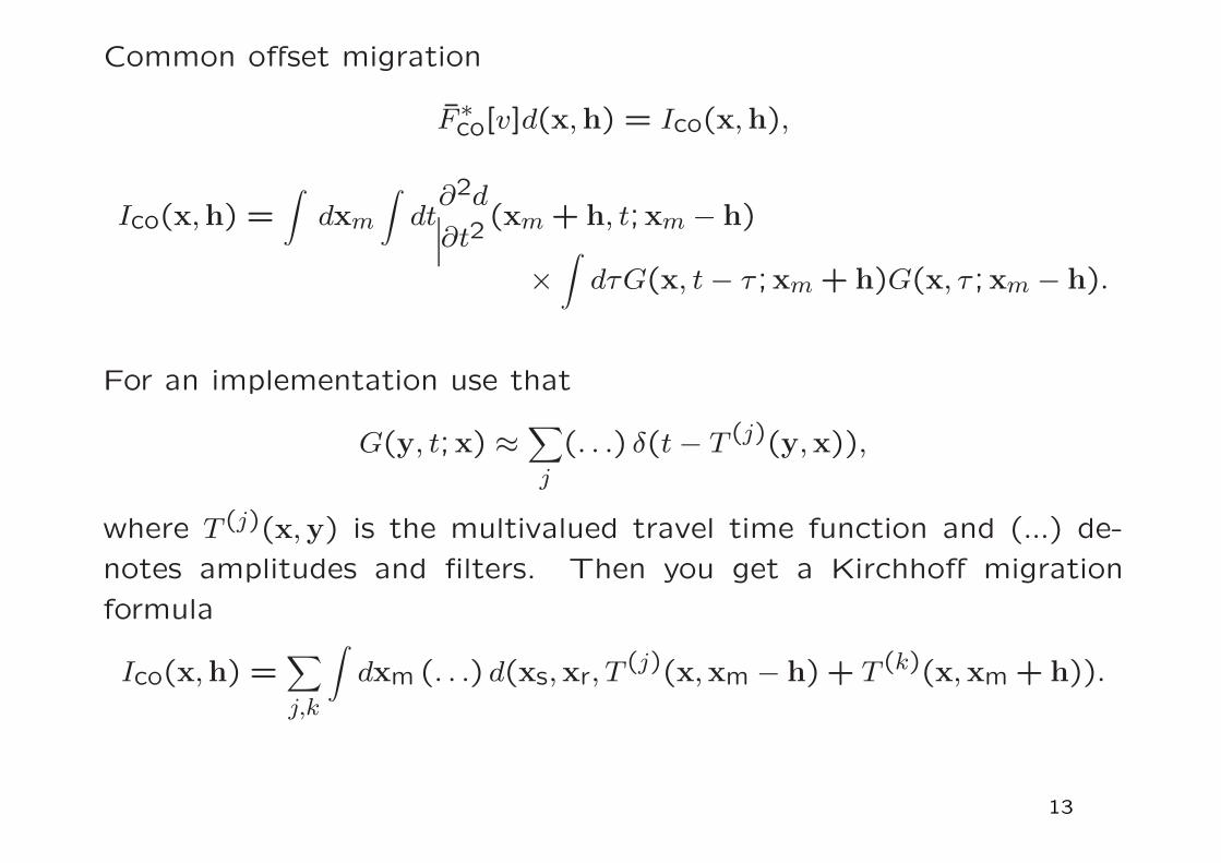
Common offset migration

F ∗co[v]d(x, h) = Ico(x, h),

Ico(x,h) =∫

dxm

∫

dt∂2d

∂t2(xm + h, t;xm − h)

×∫

dτG(x, t− τ ;xm + h)G(x, τ ;xm − h).

For an implementation use that

G(y, t;x) ≈∑

j

(. . .) δ(t− T (j)(y,x)),

where T (j)(x, y) is the multivalued travel time function and (...) de-

notes amplitudes and filters. Then you get a Kirchhoff migration

formula

Ico(x,h) =∑

j,k

∫

dxm (. . .) d(xs,xr, T(j)(x,xm − h) + T (k)(x, xm + h)).

13

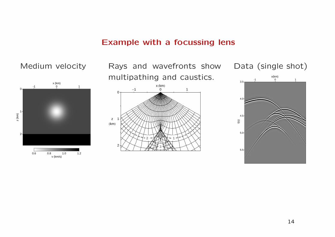
Example with a focussing lens

Medium velocity

0

1

2

z (k

m)

-1 0 1x (km)

0.6 0.8 1.0 1.2v (km/s)

Rays and wavefronts show

multipathing and caustics.

2

1

0

z

HkmL

-1 0 1x HkmL

12

3

Data (single shot)

3.5

4.0

4.5

5.0

5.5

-1 0 1x(km)

t(s)

14

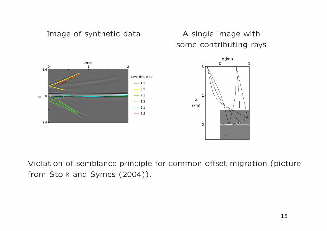
Image of synthetic data

1.6

2.0

2.4

x2

0 1 2offset

3,2

3,1

1,2

2,1

3,3

1,1

travel time # s,r

A single image with

some contributing rays

2

1

0

z

HkmL

0 1x HkmL

Violation of semblance principle for common offset migration (picture

from Stolk and Symes (2004)).

15

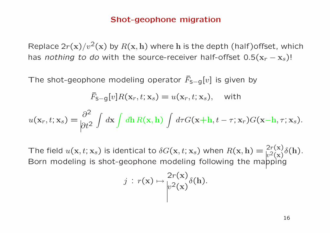
Shot-geophone migration

Replace 2r(x)/v2(x) by R(x, h) where h is the depth (half)offset, which

has nothing to do with the source-receiver half-offset 0.5(xr − xs)!

The shot-geophone modeling operator Fs−g[v] is given by

Fs−g[v]R(xr, t;xs) = u(xr, t;xs), with

u(xr, t;xs) =∂2

∂t2

∫

dx∫

dhR(x, h)∫

dτG(x+h, t− τ ;xr)G(x−h, τ ;xs).

The field u(x, t;xs) is identical to δG(x, t;xs) when R(x, h) = 2r(x)v2(x)

δ(h).

Born modeling is shot-geophone modeling following the mapping

j : r(x) 7→2r(x)

v2(x)δ(h).

16

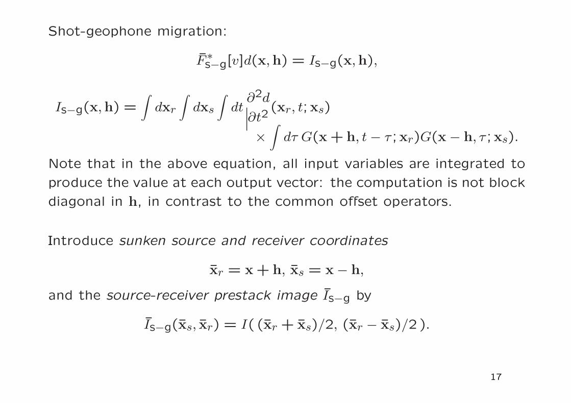
Shot-geophone migration:

F ∗s−g[v]d(x, h) = Is−g(x, h),

Is−g(x, h) =

∫

dxr

∫

dxs

∫

dt∂2d

∂t2(xr, t;xs)

×∫

dτ G(x + h, t− τ ;xr)G(x− h, τ ;xs).

Note that in the above equation, all input variables are integrated to

produce the value at each output vector: the computation is not block

diagonal in h, in contrast to the common offset operators.

Introduce sunken source and receiver coordinates

xr = x + h, xs = x− h,

and the source-receiver prestack image Is−g by

Is−g(xs, xr) = I( (xr + xs)/2, (xr − xs)/2 ).

17

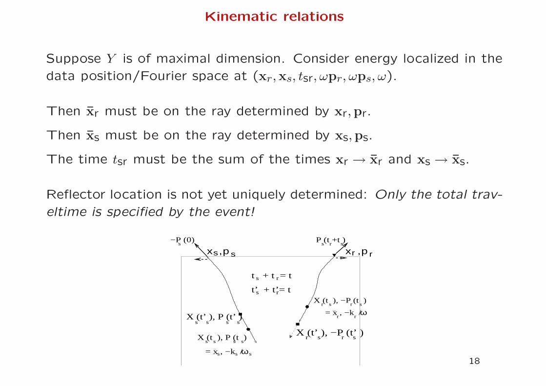
Kinematic relations

Suppose Y is of maximal dimension. Consider energy localized in the

data position/Fourier space at (xr,xs, tsr, ωpr, ωps, ω).

Then xr must be on the ray determined by xr,pr.

Then xs must be on the ray determined by xs,ps.

The time tsr must be the sum of the times xr → xr and xs → xs.

Reflector location is not yet uniquely determined: Only the total trav-

eltime is specified by the event!

X (t’ ), P (t’ )

t + t = t

t’ + t’= t

s r

s r

sX (t ), P (t )

s

s P (t +t )

r ss−P (0)

rX (t’ ), −P (t’ )

r

r r

r rX (t ), −P (t )

s

s s

sss

p sx ,s x ,r p r

s ss s

s s

ω= x , −k / s

ω= x , −k /18

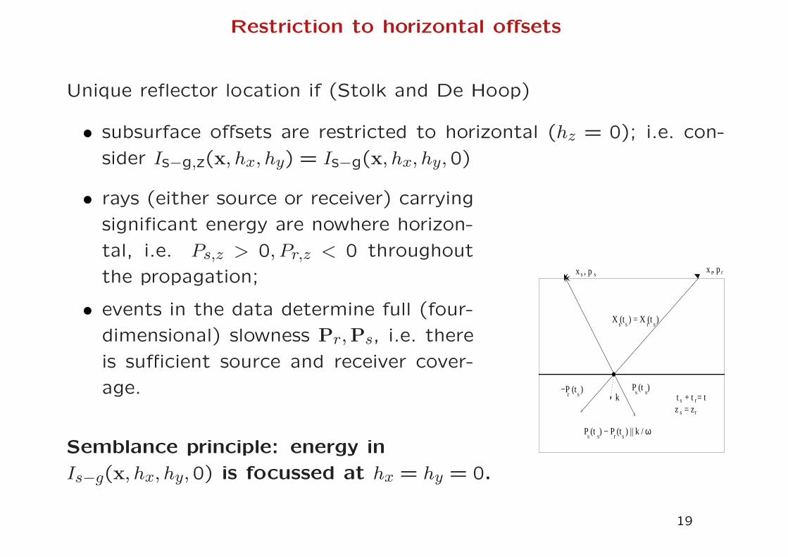
Restriction to horizontal offsets

Unique reflector location if (Stolk and De Hoop)

• subsurface offsets are restricted to horizontal (hz = 0); i.e. con-

sider Is−g,z(x, hx, hy) = Is−g(x, hx, hy,0)

• rays (either source or receiver) carrying

significant energy are nowhere horizon-

tal, i.e. Ps,z > 0, Pr,z < 0 throughout

the propagation;

• events in the data determine full (four-

dimensional) slowness Pr,Ps, i.e. there

is sufficient source and receiver cover-

age.

Semblance principle: energy in

Is−g(x, hx, hy,0) is focussed at hx = hy = 0.

r

s rx ,

X (t ) = X (t )s s

s s

s s

P (t ) − P (t ) || k /

t + t = ts r

z = zs

x

r s

−P (t )

rsp, p

P (t )k

ω

r s

r s

19

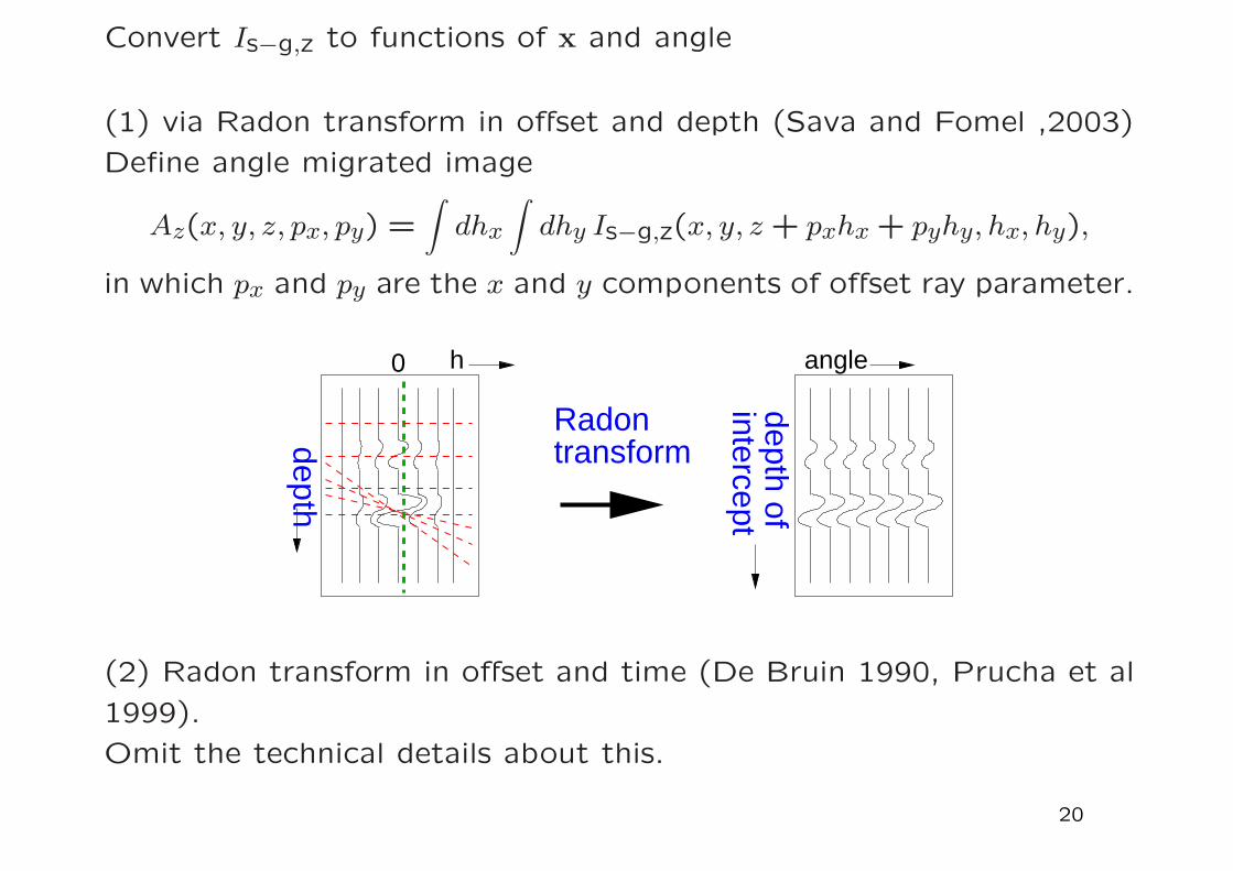
Convert Is−g,z to functions of x and angle

(1) via Radon transform in offset and depth (Sava and Fomel ,2003)

Define angle migrated image

Az(x, y, z, px, py) =

∫

dhx

∫

dhy Is−g,z(x, y, z + pxhx + pyhy, hx, hy),

in which px and py are the x and y components of offset ray parameter.

h0

interceptdepth of

angle

depth

Radontransform

(2) Radon transform in offset and time (De Bruin 1990, Prucha et al

1999).

Omit the technical details about this.

20

Examples

Compare

• Kirchhoff angle migration: Examples from Stolk and Symes, 2004

• Wave equation angle migration: From Stolk, De Hoop and Symes

(preprint 2005)

Computation: Double-square-root approach using generalized screens

(Le Rousseau and De Hoop (2001)), thanks A. E. Malcolm for

help.

21

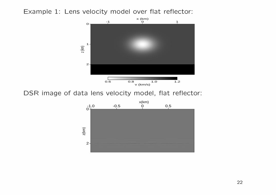
Example 1: Lens velocity model over flat reflector:

0

1

2

z (km

)

-1 0 1x (km)

0.6 0.8 1.0 1.2v (km/s)

DSR image of data lens velocity model, flat reflector:

0

2

-1.0 -0.5 0 0.5x(km)

z(km

)

22

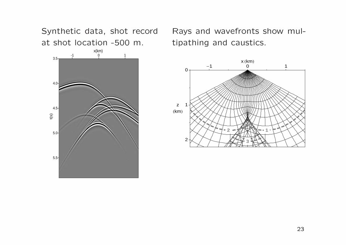
Synthetic data, shot record

at shot location -500 m.

3.5

4.0

4.5

5.0

5.5

-1 0 1x(km)

t(s)

Rays and wavefronts show mul-

tipathing and caustics.

2

1

0

z

HkmL

-1 0 1x HkmL

12

3

23

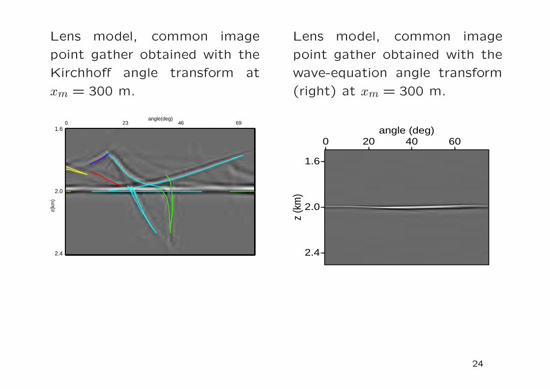
Lens model, common image

point gather obtained with the

Kirchhoff angle transform at

xm = 300 m.

1.6

2.0

2.4

0.0 0.4 0.8 1.269angle(deg)

z(km

)

0 23 46

Lens model, common image

point gather obtained with the

wave-equation angle transform

(right) at xm = 300 m.

1.6

2.0

2.4

z (k

m)

0 20 40 60angle (deg)

24

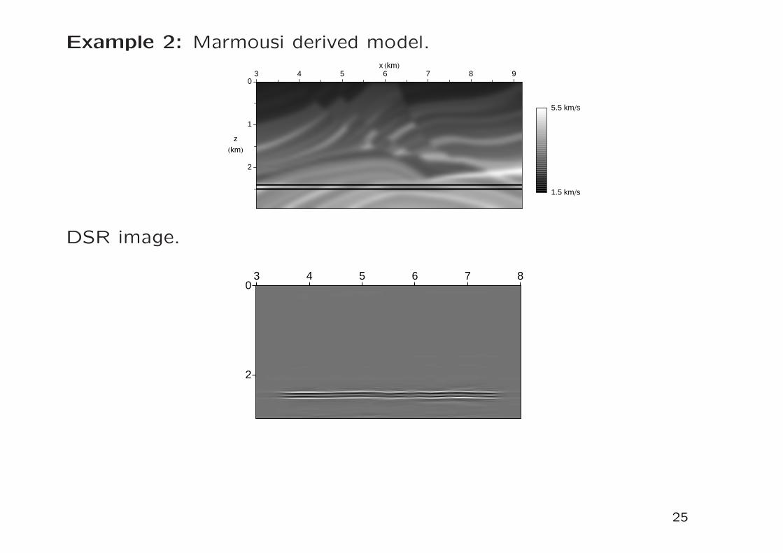
Example 2: Marmousi derived model.

2

1

0

z

HkmL

3 4 5 6 7 8 9x HkmL

5.5 km�s

1.5 km�s

DSR image.

0

2

3 4 5 6 7 8

25

2.8

2.6

2.4

2.2

2

1.8

time

HsL

5.2 5.6 6 6.4 6.8 7.2receiver position HkmL

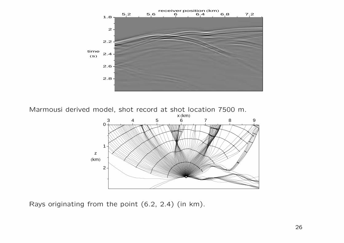
Marmousi derived model, shot record at shot location 7500 m.

2

1

0

z

HkmL

3 4 5 6 7 8 9x HkmL

Rays originating from the point (6.2, 2.4) (in km).

26

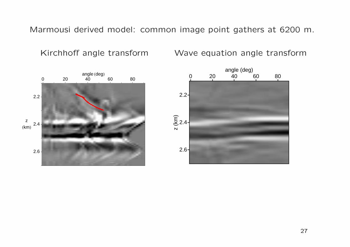
Marmousi derived model: common image point gathers at 6200 m.

Kirchhoff angle transform Wave equation angle transform

2.6

2.4

2.2

z

HkmL

0 20 40 60 80angle HdegL

2.2

2.4

2.6

z (k

m)

0 20 40 60 80angle (deg)

27

Discussion

• The two different prestack migration methods have very different

behavior in a background medium with multipathing:

– Migration of data subsets (binwise migration):

Multipathing leads to kinematic image artifacts. These were

established in examples by both geometrical analysis and com-

putation of the images.

– Shot-geophone migration:

Geometrical analysis shows the absence of artifacts under as-

sumptions of downgoing rays, and complete acquisition cover-

age. Confirmed in images of the above mentioned examples.

This method is therefore more suitable for velocity analysis in

complex media.

• In case of marine data 3-D data an assumption is needed for the

medium variations in the sparsely sampled direction.

28

Some references

Main ref for this talk:C. C. Stolk, M. V. de Hoop and W. W. Symes, Kinematics of shot-geophone mi-gration, preprint, www.math.utwente.nl/˜stolkcc.

Other refs.:Ten Kroode, A. P. E., Smit, D. J. and Verdel, A. R., A microlocal analysis ofmigration, Wave Motion, 28 (1998), pp. 149-172.

Nolan, C. J., and Symes, W. W., Global solution of a linearized inverse problem forthe wave equation: Comm. P. D. E., 22 (1997), pp. 919952.

Stolk, C. C., and Symes, W. W., Kinematic artifacts in prestack depth migration:Geophysics, 69 (2004), pp. 562575.

C. C. Stolk and M. V. de Hoop, Modeling of seismic data in the downward con-tinuation approach, SIAM Journal on Applied Mathematics 65 (2005), no. 4, pp.1388-1406

C. C. Stolk and M. V. de Hoop, Seismic inverse scattering in the downward contin-uation approach, preprint.

29