Efficient Error-Correcting Geocoding ∗

Christian Jung, Daniel Karch, Sebastian Knopp, Dennis Luxen, and Peter SandersKarlsruhe Institute of Technology, 76128 Karlsruhe, Germany

{christian.jung,sebastian.knopp}, karch@math.tu-berlin.de {luxen,sanders}@kit.edu

May 31, 2018

Abstract

We study the problem of resolving a perhaps misspelled address of a location into geographic coor-dinates of latitude and longitude. Our data structure solves this problem within a few milliseconds evenfor misspelled and fragmentary queries. Compared to major geographic search engines such as Googleor Bing we achieve results of significantly better quality.

1 Introduction

Geocoding of a location description is the process of transforming an address into a geographical coordinate.This process has been available in geographic information systems for quite some time [9] with applicationsfor example for route planning, validating customer addresses [1], or surveillance and management of diseaseoutbreaks like the yearly wave of influenza [19]. However, with its ubiquitous use in modern web services(e.g., [13, 5]), requirements have become more severe: Since most of these services are free, geocoding serversmust handle huge streams of queries at very low cost. At the same time, users expect instantaneous answers.Finally, inputs will frequently be fragmentary, contain misspelled names or specify combinations of townand street that are inconsistent with the database. A service is likely to be more popular and useful if ittolerates such imprecisions.

While companies offering such services have naturally worked on this problem intensively, we are notaware of academic work that offers the required combination of low latency, high throughput, and error-correction for large address files. Our original aim was to make reasonable methods available to a cooperatingcompany and to the academic community. However, to our own surprise it turned out that our approachachieves better solution quality than the market leaders at low costs so that it might also help the industryto improve their services.

In this paper we focus on the algorithmic aspects of the problem to map information about town andstreet to a database entry for the intended street. We do not consider the problem of resolving house numbersor producing highly accurate output coordinates. Although this has been a major focus of previous literature,e.g., [12], we view it as orthogonal to our problem since once town and street have been correctly identified,we are dealing with much more local data and hence much smaller data volumes. For example, searchingan odd house number not present in the database can often be done by a binary search in a sequence of theknown odd house numbers followed by an interpolation [11, 12]. On todays servers with many gigabytes ofRAM, it might even be possible to precompute all estimated positions of house numbers.

The paper is structured as follows. Section 2 outlines the basic index data structure. Section 3 explainsthe query algorithm, while 4 develops on a rating function to rank the matches from the query. A variantof the algorithm for the case that the address is typed into a single field is explained in Section 5. Section6 gives a data structure that resolves ambiguous town names both as a downstream computation step andin an online setting as real-time suggestions. Section 7 reports on an experimental evaluation. Last but notleast Section 8 gives conclusions.

∗Partially supported by DFG Grant 933/5-1.

1

arX

iv:1

102.

3306

v1 [

cs.I

R]

16

Feb

2011

More Related Work

Geocoded data used to cost several dollars per 1 000 records in the mid-eighties [18] and didn’t nearly providethe spatial accuracy of todays free services. At that time the use of geographic information systems waslimited to professionals only that were aware of the difficulties and limitations of the geocoding process [24].In [16], eight geocoders are compared. However, the evaluated Californian addresses are all given with highprecision including city name, ZIP code, state and street name.

Improving the quality of geocoding using approximate string matching is considered desirable in [27] butthen dismissed as too expensive.

Approximate string matching itself has been studied intensively, e.g. [23, 22] but most actually imple-mented methods match only a specific pair of strings which is infeasible for large databases. Although thereis considerable theoretical work on text indices allowing approximate matching [22, 23], there are few imple-mentations because these methods are complicated and require superlinear space. Moreover, most previouswork is on finding all matches in a single large text. We will only require matching against full entries of adictionary which is a slightly simpler problem and thus might also allow more efficient solutions. We buildon one of the few available implementations [17], but still have to overcome the problem of superlinear spaceconsumption.

Sengar et al. [25, 26] describe a system that is able to handle ill-formed queries to a certain extent. Theirsystem does not require any country-specific rule set, but exploits the underlying geometric map data toproduce a language independent representation of the data. This kind of abstraction is especially useful inareas of the world where formal address formats are non-existing, e.g., in India. However, it remains unclearhow such systems scale to large databases.

2 Index Data Structure

Our basic input data are a set T of towns and a set S of streets that are fully defined by a name and areference to a town. In this paper we use the term “town” both for a district of another place and for anindependent place. To avoid confusion we will therefore use the term city for independent places even ifthey are small. Streets belonging to multiple towns are cut into pieces belonging to a single town. Districtsadditionally contain a reference to the city they belong to.

2.1 Inverted Indices and Town Lists

We view place and street names as (very short) documents containing a sequence of tokens separated bywhite space, commas or hyphens. Thus we can use methods known from full text search to support fastgeocoding. In particular, we build two inverted indices, i.e. the town index maps tokens appearing in townnames to the towns using that token in their name and the street index maps tokens appearing in streetnames to all streets containing this token.

In addition to the above inverted index, we precompute the set towns(s) of town IDs containing a streetwith name s and also a set towns(t) of town IDs with name t. This translation to town IDs will enable usto quickly determine which combinations of town and street name correspond to actual addresses.

2.2 Ignoring Light Tokens

While indexing by token makes the index more convenient to use, it introduces a serious problem. A streetquery of the form “New Hollywood Street” will return every street that matches any of the tokens “New”,“Hollywood”, or “Street”. In fact, about 25% of all street names match the token “Street”, thereforewe would get a really big candidate set. To avoid this problem, we adapt a concept which is often used ininformation retrieval and text mining [4, 28, 8]: The inverse document frequency of a token c with respect

2

to a set M of strings (town or street names in our case) is defined as

IDF(c):= log2

∑x∈M | tokens(x)|

| {x ∈M : c ∈ tokens(x)} |

where tokens(x) is defined as the set of tokens making up string x. Tokens that occur very often in thedocument (such as “Street”) receive a lower IDF weight than those that appear only infrequently. Tokensthat receive a high weight are more helpful in identifying the correct string, because they match fewer stringsin the index.

We will use these observations to our advantage: When a user enters an address that they want to havegeographically referenced, they may leave out parts of the address that they deem irrelevant, but they willprobably enter those parts of the query that will non-ambiguously define what they are looking for. In ourexample, the user may leave out either “New” or “Street”, but they most definitely won’t leave out the token“Hollywood”, which is also the token with the highest IDF weight among those three. If we expect the userto enter the most important part of an address, it is not necessary to have said address be referenced also bythe remaining, unimportant tokens, i.e. we don’t want to find the street “New Hollywood Street” by thetoken “Street”, because we expect that the more descriptive token “Hollywood” will be entered anyway.Let

wst :=IDF(t)∑

t′∈tokens(s) IDF(t′)

be the relative weight of the token t in the string s. In our example the relative weights might be 0.31 for“New”, 0.6 for “ Hollywood”, and 0.09 for “Street”, respectively. If we decide that the query must containtokens that make up a fraction µ of the total weight, then we can ignore the lightest k tokens, if the sum oftheir weights is not greater than µ. E.g., for µ > 0.4, we can ignore the tokens “New” and “ Street”. Notethat this local definition of importance is very different from the stop words that are completely ignored insome inverted index data structures to save space. For example, suppose our database contains streets named“Rhododendron Alley” and “Alley Street” then it is likely that the index for “Alley” will contain “AlleyStreet” but not “Rhododendron Alley”. This both save space, query time, and useless candidates.

2.3 Approximate Token Indices

We also build indices supporting approximate search on the sets of tokens appearing in town names andstreet names respectively. This design decision has two crucial advantages over the more obvious choiceto have an index on the town and street names themselves. First, since the dictionaries are much smallerthan the full data base, we can afford superlinear space to some extent. For example, our German inputset contains 1.35 million streets but only 219 thousand distinct tokens for street names. Furthermore, tokenbased indices can easily handle queries that drop part of the town or street name. For example, most usersjust type “Frankfurt” when they are looking for “Frankfurt am Main”. The approximate index [17] fortoken set M with maximum error di can be queried with a string q and returns a set Mq ⊆ M of tokensthat have edit distance (Levenshtein distance) at most di.

3 Multi-Field Search

We first concentrate on the case where a query consists of two strings typed into separate fields for townname and street name. Note that in this case it is easy and largely orthogonal to allow additional fields forhouse number or ZIP code. After normalization and tokenization (Section 3.1), we try three increasinglysophisticated ways to obtain sets CT and CS of town and street candidates respectively that allow anincreasing number of errors (Section 3.2–3.4). After each of these attempts, we combine these candidate setsinto consistent candidate addresses from CT × CS . We stop as soon as we have found satisfying solutions.When at the end no reasonable solutions have been found, an empty result is returned.

3

3.1 Initialization Phase

The input strings are first scanned and transformed into a set Q of tokens and normalized to lower-case. Thisis also the place where some culture-specific preprocessing can be done. In our German implementation,there is only one such specialty: The German words for “Street”, “Lane”, . . . are sometimes used as aseparate word and sometimes as a suffix and nobody really knows which version is correct in every case.Hence, compounds with these suffixes are broken into a normal form with separate tokens. This even workswhen the suffixes are misspelled or abbreviated.

3.2 Partially Exact Town Match

Following the successful principle of “make the common case fast”, we use a simplified special treatment forthe case of a partially exact town match where at least one sufficiently rare token of a town candidate isexactly matched. If this already yields a plausible result, we stop. For example, in the query “Franfrt am

Main, Romerberg”, “Frankfurt” was misspelled. But the token “Main” is an exact match and thereforewe consider the set of towns that contain this token somewhere in their name before we look at all possibleapproximate matches. If we find a street similar to “Romerberg” in one of the candidates, we can stop.

3.3 Periphery Search

If we successfully identified partially exact town matches during the first phase, but could not match a streetin these towns with a sufficient rating, we extend the scope of exact search to the periphery : If the inputspecifies a city, we try all its districts, if it specifies a district, we try the city it belongs to and all its districts.

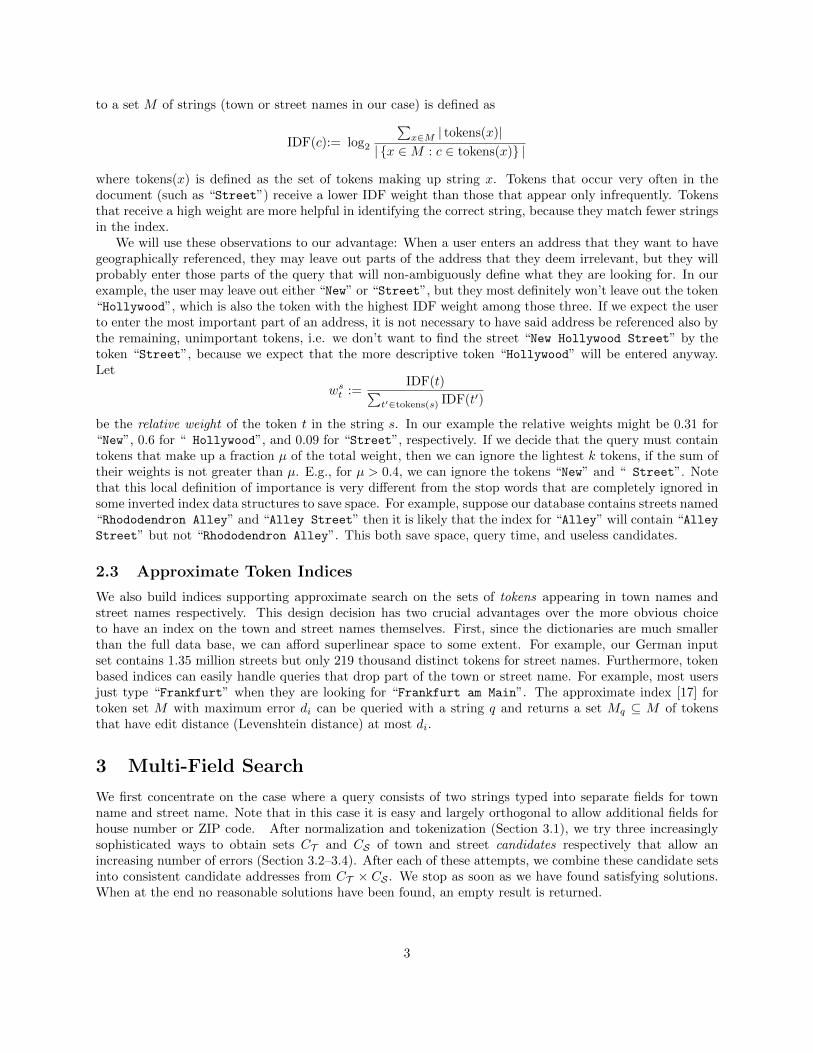
Figure 1: Two Cases of Periphery Search

If the town provided by the user is matched against a candidate x which is subsequently corrected to atown y in the periphery of x, we still calculate the rating for x, because the name of y generally does notmatch anything in the query string and would lead to a low rating.

3.4 Approximate Search

When there are no or no good partially exact matches or when even periphery search does not find a goodcandidate, additional candidates are computed using the approximate indices for towns and streets. If a towncandidate found specifies a district x of a city y, we also add y to the candidates. However, we do not do afull scale approximate periphery search because this could easily yield results that are hard to understand.

3.5 Finding Compatible Candidates

After partially exact matching, periphery search, or approximate search, that all treat towns and streetsseparately, we generate address candidates where town and street are compatible with each other. A pair

4

(t, s) ∈ CT × CS is compatible if a street with name s is present in some town with name t, i.e., we have tocompute the set

CT ×S := {(t, s) ∈ CT × CS : towns(t) ∩ towns(s) 6= ∅} .

There are various ways to do this more efficiently than the naive way of computing |CT | × |CS | set intersec-tions. Appendix A gives one particularly efficient implementation.

4 Rating Candidates

After we have dismissed most of the search space, we are left with a hopefully small set of compatible addresscandidates (t, s) ∈ T ×S. These are then rated. The result is interpreted using two threshold values ρ and ρ.Ratings below ρ are considered unsatisfactory. If all results are unsatisfactory, more extensive search is done(after partially exact matching or periphery search) or, when everything failed, an empty result is returned.In contrast, if a candidate with rating ≥ ρ is found, the search returns successfully without further attemptsat refined searching. Depending on the application we can then return the top ranked candidate or a list ofgood candidates.

To develop a rating heuristic, let us recall the different kinds of errors that we want to compensate for:

• Typing errors

• Missing or redundant tokens

• Inconsistent pairing of a street and a town.

Since periphery search and candidate filtering have already dealt with inconsistent candidates, we are leftwith the first two issues.

The first step on the way to a robust rating heuristic is to align the query to a candidate, i.e. find agood mapping from the tokens in the query to the tokens in the candidate (see Section 4.1). Based on thismapping, we then compute the actual rating.

The rating is computed separately for town and street by the same method and combined by the arith-metic mean afterwards. Hence, the following explanation details the town rating only. There is one smallasymmetry however that we call filter by edit distance: Since there are usually less candidate towns than can-didate streets, we first filter out candidates that are already unsatisfactory because they do not sufficientlywell fit the town description in the query.

4.1 Matching the Query to a Candidate

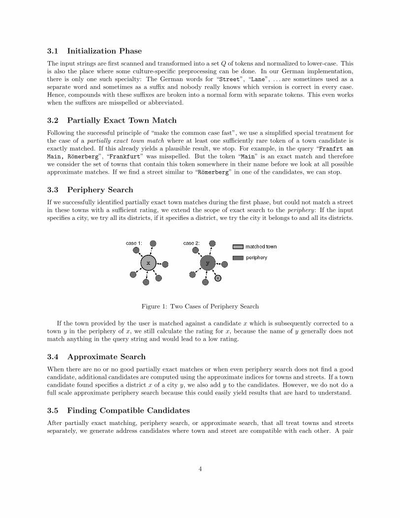
To match the town tokens q ∈ Q given by the users to the tokens of a candidate town name c ∈ C, we solve aminimum weight perfect matching problem on a bipartite graph. If |Q| ≤ |C| we add |C|− |Q| dummy nodesto Q and obtain the matching graph G = (Q∪C,Q×C) where the weight of edge (q, c) is the edit distancebetween q and c if c is not a dummy node and 0 if c is a dummy node. Edit distances take misspellings intoaccount and dummy query nodes go a long way to model missing tokens in the query. Similarly, but perhapsless importantly, if |Q| > |C| we add |Q| − |C| dummy nodes to C. This matching problem can be solvedin polynomial time (e.g. [2, 20]). Moreover, the considered graphs are very small so that solutions can becomputed quickly. See Figure 2 for an illustration.

4.2 The Rating Function

Based on the matching, we calculate a rating for each candidate. The rating should take into account thefollowing considerations:

• Each token that matches with at most d errors should be awarded some points. It makes sense tochoose d larger than the error bound di for the approximate index since space or index access time isno issue for the pairwise distance computations used for the rating function.

5

Jersey City, New York

central New York Jersy cty

1 0

0 1

Figure 2: Candidate (top) is matched against query (bottom). Edge labels symbolize edit distances.

• Tokens that could not be matched with at most d errors should not be awarded points and may evenbe punished.

• The user is more likely to omit information (either because they forget it or because they deem itunnecessary) than to over-specify the query. Therefore, tokens in the query that don’t match anythingin the candidate should be punished higher than candidate tokens that don’t match anything in thequery.

• The rating should be a real number in the interval [0, 1], with one denoting a perfect match.

• The heuristic should be able to distinguish between tokens that are important and tokens that do notprovide much information.

Rather than directly using the edit distance, we also want to take into account the lengths of comparedwords, since the rate of error that can be introduced into a word with a constant number of changes dependson its length. We therefore define token similarity between two tokens q and c as

sim(q, c) :=

{1− editDistance(q,c)

|c| , if editDistance(q, c) ≤d

0, else.

We normalize the error rate by the length of c since candidates are entries that are actually present in ourdatabase.

In order to take the importance of a candidate token into account, we use its inverse document frequency(see Section 2).

Let M denote the set of edges (d, c) between query tokens and candidate tokens that were matched withedit distance ≤ d. Let U denote the set of unmatched query tokens, i.e., those tokens that could not bematched to any candidate token with at most d errors. We can now define our rating function

rating(Q,C):= γ ratingQ(Q,C) + (1− γ) ratingC(Q,C)

where

ratingQ(Q,C):=

∑(q,c)∈M

(sim(q, c))α IDF(c)

∑(q,c)∈M

IDF(c) + |U | IDFavgand

ratingC(Q,C):=∑

(q,c)∈M

IDF(c)/∑c∈C

IDF(c)

Where IDFavg is the average over the IDF-values of all town tokens. The term |Mc| IDFavg expresses thatthe unmatched queries should have matched somewhere but we have no idea where – so we use an averageIDF-value. The parameter α is used to adjust how important it is to have similar matches. Notice that

6

ratingQ is not influenced by the number of unmatched candidate tokens. This is why we compute a convexcombination of ratingQ with ratingC which penalizes unmatched candidate tokens. The parameter γ ∈ [0, 1]specifies the relative weight. Usually we want to give more weight to the matched parts of a query, thereforewe choose γ > 1/2.

5 Single-Field Search

In the previous sections we focused on separate fields for town and street because this interface is moreimportant for our cooperation partner, because multi-field search is easier to program, and one shouldexpect that it reduces errors. From the users points of view, however, it is more convenient to enter a queryinto a single text field, with street and town in arbitrary order. Online services like Google Maps or BingMaps have therefore adopted single-field search.

However, in order to compare multi-field search and single-field search and in order to compare ourapproach with internet services, we have also implemented a simple version of single-field search with anemphasis on quality.

Our solution is based on the plausible hypothesis that the token sequence resulting from a single-fieldquery has the format streetToken∗townToken+ or townToken+streetToken∗, i.e., street and town tokens arecontiguous and there is at least one token designating a town. We exhaustively try all 2m− 1 possible waysto split a token sequence of length m and call a multi-field search for each of them. Refer to Section 8 for adiscussion of possible optimizations.

For example, the query “Oxford Street, London” can be split as

Town StreetOxford Street London

Oxford Street London

Oxford Street London

Street London Oxford

London Oxford Street

Only the last line would return a perfect rating as we might have hoped. This query is a bit lucky thoughsince there is no “London Street” in “Oxford” which, if it existed, would also receive a perfect rating.

6 Neighborhood Graph

In most countries, city names are not unique. For example, Wikipedia knows 41 Springfields, 5 of them inWisconsin. We present an efficient data structure here that can be used to find plausible nearby cities fordisambiguation. Applications could either use the data structure to propose disambiguating places or theycould match them to inputs of the user such as “Springfield near Kansas City”.

What makes a city plausible? It should be large, and it should be close to the city it is supposed todisambiguate. Hence, we are facing a bicriteria optimization problem. A safe way to handle such a situationis to consider all cities that are not dominated by any other city. (x dominates y wrt city t if it is both closerto t than y and larger than y.) This problem is known under several names: finding Pareto optima, vectormaxima [21], or a skyline [7]. If the cities are sorted by size, it is easy to solve the problem with a full scanof all cities – outputting a city if it is closer than all previously inspected ones. However, looking at all citiesmay still be too slow.

We will encode the required information into a graph. Assume the cities are numbered 1 to n bydecreasing size. There is no need to store all towns, only those cities big enough to serve as a referenceplace. A convenient way to define the size of a city here is to just count the number of streets. LetDi:= ({1, . . . , i} , Ei) denote the Delaunay triangulation1 [10] of the i largest cities.

1Note that for convenience we work with Euclidean geometry here. It is an interesting problem to consider what happenswhen we do geometry on the surface of a sphere.

7

Then we will consider the neighborhood graph D∗:= ({1, . . . , i} ,∪ni=1Ei). Depending on the application,we may interpret D∗ as a directed acylic graph where all edges go from smaller to larger indices (downward)or vice versa (upward). The intuition here is that the Delaunay triangulation encodes a natural concept ofproximity. Directing the edges upward, i.e., towards larger cities allows us to find such cities. Obviously, itis not enough to just consider the Delaunay triangulation Dn of all n cities since we would usually end upin a dead end of a medium sized cities whose neighbors are all smaller. The following theorem states thatthe union D∗ of n Delaunay triangulation solves this problem very effectively:

Theorem 1 Consider any map position (x, y). The Pareto optima with respect to city size and closeness toposition (x, y) forms a downward path from node 1 to the city closest to (x, y). Moreover, this path can befound with the simple greedy algorithm depicted in Figure 3.

Proof 1 By induction from 1 to n, analogous to the work of Birn et al. [6].

Of course it is important how long it takes to construct D∗ and how much space it takes. If the size ofa city is assumed to be independent on its position, the problem is the same as in randomized incrementalconstruction of a Delaunay triangulation [14] – we get a linear number of edges in time O(n log n).

7 Experimental Evaluation

Implementation We have implemented the system described above in C++ making extensive use of theSTL library. This probably leaves open significant further tuning opportunities. For example, we use a simplemerging based STL algorithm for computing set intersections rather than a tuned code as used in full textindices. The tuning parameters have been chosen intuitively without an attempt at finding optimal values:We ignore light tokens comprising up to 40 % of the cumulative IDF of a name. The correction limit of theapproximate dictionaries and pairwise edit distance computations is limited to d = di = 2 in order to keepspace consumption low. Candidate matching use the Hungarian method [2] using the implementation by [3].In the rating function, similarities between matched words are taken to the power α = 2 and in the convexcombination ratingQ(Q,C) = γ ratingQ(Q,C) + (1− γ) ratingC(Q,C) we choose γ = 3/4. The threshold fora satisfactory rating is ρ = 1/2 and a good rating starts at ρ = 4/5. Experiments were performed on an IntelCore i7 920@2.67GHz with 12GB RAM on Linux 2.6.27 using a single core. The programs were compiledwith GCC 4.3.2.

Map Data We use commercial data (from 2009) comprising all German street and town names. There areabout 12 000 cities, 108 000 towns, 80 000 town names, 76 000 town name tokens, 1 350 000 streets, 560 000of which contain the token “Strasse”, 444 000 street names, and 269 000 street name tokens. A street nameconsists of 2.5 tokens on average, while town names consist of 1.1 tokens on average. The input data takes

Procedure PareteOptima(q)u:= 1 // start at top of hierarchy.repeat

output uforeach neighbor v of u in D∗

with u < v in increasing order doif ||q − position(v)||2 < ||q − position(u)||2 then

u:= vbreak for loop

until no closer node found

Figure 3: Finding Pareto optimal cities in the neighborhood graph D∗.

8

about 30 MB space while our index data structures take about 327 MB. A more frugal assignment of spaceto various hash tables could reduce that to a bit more than 200 MB but we think that 327 MB is almostnegligible for a server setting – even very energy-efficient 32-bit servers based on Atom, or ARM could beused.

7.1 Pseudorealistic Random Queries

For our experiments, we use a set of existing, relevant addresses R, and a set of non-existing, irrelevantaddresses I. A relevant address is sampled by first choosing a random street name s and then picking arandom town from towns(s). An irrelevant is composed of randomly chosen town and street names such thatcombination which accidentally occur in the database are rejected. Ideally, we would like to return correctresults for relevant address queries and no result for irrelevant address queries. To generate a simple randomquery, it would be easiest to just insert, delete or substitute random characters in an existing address. Theerrors that are introduced this way, however, are unlikely to resemble the errors that a human would makewhile entering a query through a keyboard. We identify several sources of errors to generate input sets withmore realistic errors.

Typing errors are very common and we distinguish

• swapped characters

Example: “Frankfurt” → “Frankfrut”

• missing characters

Example: “Frankfurt” → “Franfurt”

• superfluous or wrong characters, mostly closely located to the correct character on the keyboard (herein terms of the German QWERTZ-layout).

Example: “Frankfurt” → “Frankdfurt” or “Frankdurt”

Depending on the respective language there are several sources of error that are phonetic.

• doubled characters where there should be a single character

Example: “Dublin” → “Dubblin”

• single character where there should be two of the same

Example: “Cardiff” → “Cardif”

• The Soundex algorithm identifies classes of characters such that different characters from the sameclass differ only slightly in their pronunciation.

Example: z ≡ s, “Zaragoza” → “Saragosa”

• Two consecutive vowels that occur in the same syllable are called a diphthong. In German, for example,several different diphthongs sound the same or similar:

– ei ≡ ey ≡ ay ≡ ai

– eu ≡ au ≡ oy ≡ oi

– . . .

Example: Hoyerswerda → Heuerswerda

In order to introduce k errors into an address, we introduce dk/2e errors into the street string and bk/2cerrors into the town string. To introduce an error, we first pick a random error class, then a random token,and then a random position. All distributions are uniform.

Here we report experiments on 1 000 relevant and 100 irrelevant addresses. We classify the results returnedby the index as follows:

9

Multi-field searchrelevant irrelevant

Errors TP FN II TN FP Time [ms]0 1 000 0 0 93 7 3.021 989 10 1 95 5 2.752 988 11 1 94 6 2.443 928 66 6 94 6 2.404 854 140 6 99 1 1.795 557 431 12 97 3 1.59

Single-field searchrelevant irrelevant

Errors TP FN II TN FP Time [ms]0 1 000 0 0 52 48 26.071 989 10 1 63 37 23.332 986 13 1 74 26 19.723 927 66 7 75 25 18.444 856 125 19 80 20 16.695 560 414 26 86 14 14.31

Table 1: Matching rates and query times for random addresses – 1 000 relevant ones and 100 irrelevant ones.

• True Positive (TP): A relevant address that is correctly identified.

• True Negative (TN): An irrelevant address that does not return a result or a correct partial result (i.e.the correct town).

• False Positive (FP): An irrelevant address where the index does return a result.

• False Negative (FN): A relevant address where we don’t find a result.

• Incorrectly Identified (II): A relevant address that returns an incorrect result, i.e. another relevantaddress.

The match rates, along with the query times, are shown in Table 1.Multi-field search works extremely well, both with respect to result quality and query time. Only at

five errors, when three errors are introduced into the street name, we see a sharp increase of false negativeresults. At this point, the approximate street index will often fail to find the right result because its errorlimit is set to di = 2. Interestingly, query times decrease with the number of errors. The reason is that wehave to check a smaller number of candidates both in the approximate index and when rating candidates.

Single-field search for relevant addresses works almost as well as multi-field search. The only noticabledifference is that a small fraction of the false negative results mutates into incorrectly identified results. Forirrelevant addresses, our current implementation seems to be too aggressive though because it returns asignificant number of false positives. On the first glance it looks paradoxical that we get a larger numberof output errors when there are no spelling errors in the input. But the reason is simple: without spellingerrors we obtain higher ratings for the generated candidates and thus it becomes more likely that the result isaccepted. This indicates that the result quality could be improved by increasing the threshold for acceptinga result. Single-field query times are an order of magnitude larger than for multi-field search. This isnot surprising, since our current implementation naively factors a single-field search into several multi-fieldsearches.

Figure 4 shows the distribution of query times for the same set of 5× 1 100 queries. 90% of all multi-fieldqueries finish in less than 5 ms. The maximum query time observed is 106 ms. Note that for the serverscenario we are considering, we want very low average query time to achieve high throughput and low cost.

10

0 10 20 30 40 50 60 70 80 90

100

1 10 100 1000

% o

f que

ries

com

plet

ed

query time [ms]

0 errors1 error 2 errors3 errors4 errors5 errors

0 10 20 30 40 50 60 70 80 90

100

1 10 100

% o

f que

ries

com

plet

ed

query time [ms]

0 errors1 error

2 errors3 errors4 errors5 errors

Figure 4: Query times of single-field (left) and multi-field (right) search for several numbers of distortions.

d Bing Google Ours

0 87 97 1001 78 54 982 71 3 983 59 3 944 55 2 86

Table 2: number of resolved queries

Occasional slower queries are no problem as long as they do not lead to noticable delays for the user. 100ms is well below the delays users are accustomed to experience due to network latencies anyway. Althoughsingle-field search is an order of magnitude slower on the average, this slow-down does not translate intoa proportional increase of the slowest query times – we still remain below 406 ms. This indicates that thequery times of the generated multi-field subqueries are not strongly correlated.

We also compared against existing geocoders. To do so, we took the first 100 relevant queries fromthe above query set and ran them against the publicly available APIs2 of Bing and Google Maps. Table 2reports on the number of true positive results. Google works very well for undistorted inputs – the threeremaining errors could perhaps be attributed to differences in the input data. But already for a single error,the recognition rate drops to 54 % and completely collapses for d ≥ 2. Bing already has significant deficitsat d = 2 but fails more gracefully for distorted inputs. Still, the number of failed answers is an order ofmagnitude larger than for our system.

7.2 Real-world Queries

To get an impression of the quality of the results, we also did experiments with real-world input, i.e. actualqueries that have been provided by users of an existing geocoder3. The test data consists of multi-field 1 383queries that were logged from the the users of a cooperating company. The results were pre-classified by thecompany into five categories. We briefly describe the categories.

Exact: Queries where each token can be matched without errors to a token in the result. The differencesallowed between query and result are those that are handled by a normalization phase.

Example: “london tally road” → “London, Tally Road”Partially Exact: Queries where each token occurs in the result, but not each token of the result string

occurs in the query.

2It should be noted that the subjective performance of Google with interactive use on Google-Maps is much better thanover the API. In particular, the auto-completion mechanism works very well but is obviously not applicable to the API.

3Complete references will be given in the final version of paper.

11

Bing Google OursClass # s w n s w n s w nExact 100 81 5 24 100 0 0 100 0 0Partial 99 77 20 2 96 2 1 99 0 0High 81 60 16 5 65 10 6 77 2 2Medium 34 7 1 26 16 11 7 27 6 1Low 15 1 1 12 9 4 2 13 1 1

Table 3: The match rates of our geocoder on real-world queries.

Example: “london tally” → “London, Tally Road”High/Medium/Low: Queries that contain errors. The labels High, Medium, and Low were assigned

depending on the “confidence” of the old geocoder to have a correct interpretation of the input.

Example: “Lodon; Tall Rd” → “London, Tally Road” (e.g. classified as Medium )We tested our address search with these queries checking correctness of our result manually. We classify

the results into three categories:Strong Match: A result that is unquestionably correct. In many cases the query was non-ambiguous

and easy to verify.Weak Match: A result that is not correct, but has successfully identified parts of the query, e.g. the

town.No Match: Either a result that is definitely incorrect, or no result at all.In total, the test data consists of 1 383 queries, classified into 844 Exact, 357 Partially Exact, 125 High,

41 Medium, and 16 Low queries. Since they had to be verified by hand, we picked random samples of atmost 100 queries per class. Also, we removed those that were not resolvable (e.g. for shopping centers, waterparks etc. – our index does not contain points of interest). There remained 100 exact and 99 partially exactqueries, as well as 81, 34 and 15 queries classified as high, medium and low. The results are shown in Table3.

Our system outperforms the Google and Bing API in all categories. As with the real world inputs,Google is similarly good for (partially) exact queries but looses ground for errorneous inputs. For example,for category High our system returns correct results for all but 4 of the inputs whereas Google fails for 16inputs – a factor four in the failure rate. An interesting difference to the random inputs is that now Googleconsistently outperforms Bing – also for the inputs with errors.

7.3 Parameters that affect the Query Time

We use several techniques to make sure that the number of candidates stays small and that we don’t haveto perform too many edit distance computations. To see if these techniques are necessary and how each ofthem affects the query time, we have performed a number of of experiments. The techniques are:

Filter Incompatible Candidates (FIC): As described in Section 3.5, we keep only those town andstreet candidates that are geographically compatible.

Filter by Edit Distance (FED): As described in Section 4 we have an additional filtering stagebefore full rating evaluation the drops candidates that can already eliminated because the town names arean unsatisfactory match.

Ignore Light Tokens (ILT): As described in Section 2, we can ignore some tokens during the construc-tion of the index due to their weight in comparison to the other tokens. E.g. the candidate “New Hollywood

Street” will be represented only by “Hollywood”, because the other two tokens occur so frequently in thedictionary that they would not be of much help to distinguish this candidate from others.

As we can see in Table 4, disabling ILT absolutely destroys the performance. To see why this is so,consider the most frequent token in the street dictionary, “street”. If we randomly choose any street, theprobability that it contains the token “street” is about 1/3. Without ILT, any query that contains thetoken “street” will return all candidates that contain this token. Hence, if we randomly choose a candidate

12

ILT FIC FED Query Time [ms]

× × × 570.00× × X 566.00× X × 199.00× X X 126.00X × × 10.68X × X 10.58X X × 3.45X X X 2.09

Table 4: The effect of the features ILT, FIC and FED on the lookup time.

and query the index with this candidate, we can expect a candidate set that contains at least 1/9 of allstreets, which is almost 50 000 candidates for our data. In our experiments the actual number of candidateswas even bigger, 67 000 candidates on average. The query time drops by a factor of almost 100 when weenable ILT. FIC gives us another boost of factor 3 and FED makes a difference only when used in conjunctionwith FIC. None of these features has a noteworthy effect on the memory requirements of the index, thereforeall of them should be enabled by default.

7.4 Neighborhood Graph

We have build a neighborhood graph for all 12 379 cities in our input, resulting in 71 896 edges, i.e., thereare less than 6 edges per node which is similar to what we would expect for random city sizes. About 290nodes are reachable from a city on the average, saving a factor > 40 compared to a full scan of the city table,even if we do not fully use Theorem 1.

We also performed a small user study to test our model. We randomly picked 48 towns from a map ofGermany and asked a non-expert in the field of geography or computer science to attribute a larger referencetown to the one we picked. In 46 of these cases, a Pareto-optimal reference town was chosen.

8 Conclusions and Future Work

We presented algorithms and data structures for error-correcting geocoding that yield instantaneous answersat costs negligible compared to the overheads for displaying maps answers, etc. over the internet. Perhapsmost surprising is that we still have a high match rate with as much as four errors and this is much betterthan current web geocoders. Another pleasant surprise was that our combination of powerful data structuresand general rating functions yields a considerably simpler solution than several rule based industrial solutionswe have heard about.

Although we are already quite fast, we still have significant tuning opportunities. In particular, it will berelatively easy to further speed up single-field search. For example, we currently do not even cache accessesto the approximate dictionary or results edit distance computations. More generally, faster algorithms foredit distance computation could be tried [15].

Although our experiments have so far focused on commercial German road data, we believe that they areeasy to adapt to other Western industrial countries. In particular, these countries have similar address sys-tems and language conventions. Points of interest (POI) like gas stations or restaurants can be incorporatedby treating them like a street, town or house number depending on the context. Finding street intersectionsis relatively easy once we have geocoded the two intersecting streets.

The basic ingredients – fast approximate dictionary search, token matching and scoring functions mightalso help in other settings like in countries with more complicated addresses or less structured reference data.However in that case we should expect more errors, longer query times, and the need for further heuristics.

13

Our concept of neighborhood graph is a promising approach to disambiguate queries involving frequenttown names. One interesting aspect is that the set of nodes reachable through the neighborhood graph D∗

may contain further “interesting” nodes. In particular, we may want to restrict the set of reported cities tothose in the same “region” (e.g., county, state, or nation) as the query town. Since Delaunay triangulationsencode neighbors “in all directions”, we suspect that with appropriately defined “locally well behaved regionshapes” the desired output still consists of nodes reachable in D∗.

References

[1] C. C. A. Tang. ArcGIS9 Geocoding Rule Base Developer Guide. ESRI, 2003.

[2] R. Ahuja, T. Magnanti, and J. Orlin. Network Flows : Theory and Algorithms. Prentice-Hall, 1993.

[3] An implementation of the Kuhn-Munkres Assignment Algorithm.http://code.google.com/p/hungarianassignment/.

[4] R. Baeza-Yates and B. Ribeiro-Neto. Modern Information Retrieval. ACM Press / Addison-Wesley,1999.

[5] Bing Maps. http://maps.bing.com.

[6] M. Birn, M. Holtgrewe, P. Sanders, and J. Singler. Simple and fast nearest neighbor search. InProceedings of the Twelfth Workshop on Algorithm Engineering and Experiments, ALENEX 2010, pages43–54, 2010.

[7] S. Borzsonyi, D. Kossmann, and K. Stocker. The skyline operator. In 17th International Conference onData Engineering (ICDE’ 01). IEEE, 2001.

[8] S. Chaudhuri, K. Ganjam, V. Ganti, and R. Motwani. Robust and efficient fuzzy match for online datacleaning. In ACM SIGMOD International Conference on Management of data, 2003.

[9] D. Cooke. The History of Geographic Information Systems: Perspectives from the Pioneers. PrenticeHall, 1998.

[10] M. de Berg, M. van Kreveld, M. Overmars, and O. Schwarzkopf. Computational Geometry Algorithmsand Applications. Springer-Verlag, 2nd edition, 2000.

[11] W. J. Drummond. Address matching: GIS technology for mapping human activity patterns, 1995.

[12] D. W. Goldberg, J. P. Wilson, and C. A. Knoblock. From text to geographic coordinates: The currentstate of geocoding. Journal of the Urban and Regional Information Systems Association, 19, 2007.

[13] Google Maps. http://maps.google.com.

[14] L. J. Guibas, D. E. Knuth, and M. Sharir. Randomized incremental construction of Delaunay andVoronoi diagrams. Algorithmica, 7(4):381–413, 1992.

[15] H. Hyyro, K. Fredriksson, and G. Navarro. Increased bit-parallelism for approximate string matching.ACM Journal of Experimental Algorithmics, 10, 2005.

[16] J. P. W. J. N. Swift, D. W. Goldberg. Geocoding best practices: Review of eight commonly usedgeocoding systems. Technical report, University of Southern California GIS Research Laboratory, 2008.

[17] D. Karch, D. Luxen, and P. Sanders. Improved fast similarity search in dictionaries. In E. Chavezand S. Lonardi, editors, String Processing and Information Retrieval, volume 6393 of Lecture Notes inComputer Science, pages 173–178. Springer Berlin / Heidelberg, 2010.

14

[18] N. Krieger. Overcoming the absence of socioeconomic data in medical records: validation and applicationof a census-based methodology. Am J Public Health, 82, 1992.

[19] N. Krieger, J. T. Chen, P. D. Waterman, M. J. Soobader, S. V. Subramanian, and R. Carson. Geocodingand monitoring of us socioeconomic inequalities in mortality and cancer incidence: does the choice ofarea-based measure and geographic level matter?: the public health disparities geocoding project. AmJ Epidemiol, 156, Sep 2002.

[20] H. W. Kuhn. The Hungarian method for the assignment problem. Naval Research Logistic Quarterly,2, 1955.

[21] H. T. Kung, F. Luccio, and F. P. Preparata. On finding the maxima of a set of vectors. J. ACM,22(4):469–476, 1975.

[22] G. Navarro, R. Baeza-yates, E. Sutinen, and J. Tarhio. Indexing methods for approximate stringmatching. IEEE Data Engineering Bulletin, 24:2001, 2000.

[23] G. Navarro and E. Chavez. A metric index for approximate string matching. Theor. Comput. Sci.,352(1):266–279, 2006.

[24] D. Roongpiboonsopit and H. A. Karimi. Comparative evaluation and analysis of online geocodingservices. International Journal of Geographical Information Science, 24, 2010.

[25] V. Sengar, T. Joshi, J. Joy, S. Prakash, and K. Toyama. Robust location search from text queries.In GIS ’07: Proceedings of the 15th annual ACM international symposium on Advances in geographicinformation systems, 2007.

[26] V. Sengar, T. Joshi, J. M. Joy, and S. Prakash. Building a global location search service. In SIGMOD’08: Proceedings of the 2008 ACM SIGMOD international conference on Management of data. ACM,2008.

[27] W. Winkler. Approximate string comparator search strategies for very large administrative lists. InProceedings of the Section on Survey Research Methods, pages 4595–4602, 2004.

[28] H. C. Wu, R. W. P. Luk, K. F. Wong, and K. L. Kwok. Interpreting tf-idf term weights as makingrelevance decisions. ACM Trans. Inf. Syst., 26(3):1–37, 2008.

A Fast Computation of CT ×S

We describe this algorithm in an appendix since it is an application of folklore tricks in maintaining sets ofsmall integers and thus not a really new result. On the other hand, the applications of these tricks may notbe obvious in this case so that a description is sensible. We first compute the union towns(CS) of all setstowns(s) for s ∈ CS . towns(CS) is represented as an array A with one entry for each town ID.4 While doingthis, we annotate each entry of towns(CS) with a list ` of pointers to the street names that enter this towninto the union. Then, for each t ∈ CT and each x in towns(t) we remember {(t, s) : s ∈ A[x].`} as compatiblecandidates. The algorithm is linear in the size of the inspected lists towns(t), towns(s), and the output size.

4A is initialized only once during program startup. Afterwards it suffices to clean entries that have actually been used. Tofacilitate this, the used town IDs are stored in a stack.

15