Shannon capacity-constrained behavior

Christopher A. Sims

June 20, 2014

Outline

Intro

Examples

Macro stylized facts

I For macro time series that are not auction-market prices andare not linked by accounting identities, typical impulseresponses show a substantial weight at zero lag for ownshocks, but a smooth hump shape for cross-variable shocks.

I To explain the smooth hump shapes, economic modelersintroduce “adjustment costs”, which have no clear connectionto anything measurable in microeconomic data.

I The adjustment costs themselves imply that own-responsesshould also be smooth. Thus additional shocks, that changechoice variables without incurring adjustment costs, are alsorequired.

Micro stylized facts

I Most people, most of the time, do not respond immediately toprice signals, and indeed may not even be fully aware of pricechanges.

I For example: A person driving down Route 1 in New Jerseyhas dozens of opportunities to buy gas, at prices that areposted on large signs so she can see them as she drives by.

I A fully rational agent would keep track of the pricedistribution and the amount of gas in the gas tank,continually re-optimizing to decide where to buy gas.

I An actual person probably is listening to the radio and talkingwith her companions instead, stopping to buy gas at the firststation to show up when the low-gas signal lights up, so longas the price doesn’t look too outrageous.

Micro stylized facts

I Most people, most of the time, do not respond immediately toprice signals, and indeed may not even be fully aware of pricechanges.

I For example: A person driving down Route 1 in New Jerseyhas dozens of opportunities to buy gas, at prices that areposted on large signs so she can see them as she drives by.

I A fully rational agent would keep track of the pricedistribution and the amount of gas in the gas tank,continually re-optimizing to decide where to buy gas.

I An actual person probably is listening to the radio and talkingwith her companions instead, stopping to buy gas at the firststation to show up when the low-gas signal lights up, so longas the price doesn’t look too outrageous.

Information processing costs: Shannon’s measure

I It seems realistic to recognize that even freely availableinformation is sometimes ignored, because processing it is insome sense costly.

I An economist wants to include this cost in the rationalagent’s decision problem.

I But how to measure such a cost? Shannon had an answer.

I If you believe information flow should be modeled as reducinguncertainty about some random quantities, and if you believethat information flows from observing two random quantitiesin succession should “add up” to the amount in the tworandom quantities observed jointly: You end up withShannon’s measure.

Information processing costs: Shannon’s measure

I It seems realistic to recognize that even freely availableinformation is sometimes ignored, because processing it is insome sense costly.

I An economist wants to include this cost in the rationalagent’s decision problem.

I But how to measure such a cost? Shannon had an answer.

I If you believe information flow should be modeled as reducinguncertainty about some random quantities, and if you believethat information flows from observing two random quantitiesin succession should “add up” to the amount in the tworandom quantities observed jointly: You end up withShannon’s measure.

Information processing costs: Shannon’s measure

I It seems realistic to recognize that even freely availableinformation is sometimes ignored, because processing it is insome sense costly.

I An economist wants to include this cost in the rationalagent’s decision problem.

I But how to measure such a cost? Shannon had an answer.

I If you believe information flow should be modeled as reducinguncertainty about some random quantities, and if you believethat information flows from observing two random quantitiesin succession should “add up” to the amount in the tworandom quantities observed jointly:

You end up withShannon’s measure.

Information processing costs: Shannon’s measure

I It seems realistic to recognize that even freely availableinformation is sometimes ignored, because processing it is insome sense costly.

I An economist wants to include this cost in the rationalagent’s decision problem.

I But how to measure such a cost? Shannon had an answer.

I If you believe information flow should be modeled as reducinguncertainty about some random quantities, and if you believethat information flows from observing two random quantitiesin succession should “add up” to the amount in the tworandom quantities observed jointly: You end up withShannon’s measure.

Shannon’s measure is all around us

I We’re used to measuring he speed of an internet connectionin megabits per second: This is a measure of the maximal rateof information flow over the connection, in Shannon’s units.

I It is usable across arbitrary variations in hardware — onedoesn’t need to know whether the connection is fiber, coaxcable, wireless, etc.

I This is one reason it is promising for economic modeling — itabstracts from the detail of people’s “hardware”.

Shannon capacity constraint’s generic implications fordynamics

I With a capacity constraint preventing full adjustment of adecision variable x to a target y , we find that the relationbetween y and x differs from the unconstrained case exactlyalong the lines of the macro stylized facts.

I The own-responses must be less smooth than the y to xresponses if the rate of mutual information flow between yand x is finite.

I These ideas were laid out in my 2003 JME paper.

This paper

I Authors: Junehyuk Jung, Jeong-Ho Kim, Filip Matejka, andChris Sims

I Subject: Understanding economic behavior with aninformation-processing constraint in non-Gaussian, non-LQcases.

I Results: In broad classes of cases, the information constraintconverts continuously distributed optimizing behavior intobehavior that is either entirely discretely distributed or isdistributed over a lower-dimensional set than theunconstrained behavior.

The static information-constrained decision problem

maxf ,µx

∫U(x , y)f (x , y)µx(dx)µy (dy)

− α−1(∫

log(f (x , y))f (x , y)µx(dx)µy (dy)

+

∫log(∫

f (x , y ′)µy (dy ′))f (x , y)µx(dx)µy (dy)

)(1)

subject to

∫f (x , y)µx(dx) = g(y) , a.s. µy (2)

f (x , y) ≥ 0 , all x , y , (3)

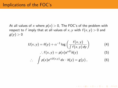
Implications of the FOC’s

At all values of x where p(x) > 0, The FOC’s of the problem withrespect to f imply that at all values of x , y with f (x , y) > 0 andg(y) > 0

U(x , y) = θ(y) + α−1 log

(f (x , y)∫f (x , y) dy

)(4)

∴ f (x , y) = p(x)eαUh(y) (5)

∴∫

p(x)eαU(x ,y) dx · h(y) = g(y) , (6)

The function C (x) =∫eαU(x ,y)h(y) dy

I It has to be one whenever p(x) > 0, because for these valuesof x it is the integrand is the conditional pdf of y | x .

I So B = {x | C (x) = 1} contains the support of x .

I If the objective function U is analytic in x on an open set S , itis often easy to show that C (x) is also analytic in x .

I Then B is either the whole of S or it contains no open sets.When S is one-dimensional, B is either the whole of S or acountable collection of points with no limit points in S .

Outline

Intro

Examples

Monopolist with random costs

I x is price; y is unit cost.

I U(x , y) = q(x) · (x − c)

I Say q(x) = a− bx and x restricted to (0, a/b).

I Then price has a distribution with support a finite set ofpoints within (0, a/b)

I This model was solved numerically in earlier work by Matejka,where the discreteness was apparent.

What the pricing model might explain

I Micro data on prices show that for a given product they tendto remain constant for a while, but jump around between afinite set of values.

I If Shannon information-processing costs were the explanation,this would suggest not trying to connect the frequency ofprice adjustments to any measurable physical “menu cost”.

Portfolio choice

I Fixed wealth of 1 to be allocated over a risk free asset and acollection of risky assets with yields z = y + ε

I x : portfolio weights (sum to one)

I ε: “hard” uncertainty; information-processing can’t reduce it.Only y is reducible.

I U(x , y) = Eε[V (x ′y)]

Results for quadratic utility, Gaussian randomness

I This is not an “LQ” problem, because objective is a quadraticfunction of a quadratic.

I We can show analytically that the solution concentrates on aset of less than two dimensions.

I We assume two risky assets, with yields independent of eachother and identically normally distributed, plus a riskless asset.

I The plots show weights on the two risky assets.

Interpretation of results

I At high information costs, the agent just chooses to go longor short risky assets, keeping the weights on the two fixed.

I At moderate information costs, the weights are distributedover four points, corresponding to relatively long or short riskyasset 1 and long or short risky assets generally.

I At low information costs the risky asset weights distribute ona circle. Note that this implies that the riskless asset has au-shaped pdf, so that there is still a tendency for portfolios tobe at the extremes of being long or short on risk.

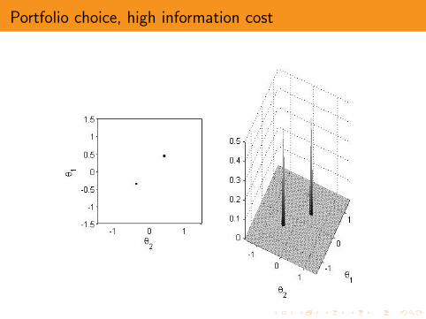
Portfolio choice, high information cost

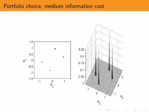
Portfolio choice, medium information cost

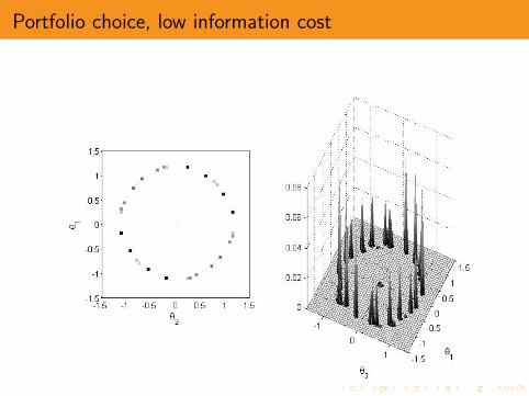
Portfolio choice, low information cost

Linear-quadratic tracking

maxE [−(x − y)′A(x − y)− θI (x , y) subject to

y ∼ N(0,Σ)

I (x , y) = 12 log |Σ| − 1

2 log |Var(y | x)|= 1

2 log |Σ| − 12 log |Σ− Var(x)|

Certainty-equivalence: optimally, E [y | x ] = x . It will be optimalto have x jointly normally distributed with y . Of course withoutthe information constraint, y ≡ x , so x ∼ N(0,Σ) and itsdistribution has the whole space as support.

Low-dimensional behavior

I When y and x are one-dimensional, if θ is high enough, it willbe optimal to collect no information, so Σ = Var(y | x) andthe distribution of x is degenerate, concentrated on the pointx = E [y ].

I When θ becomes small enough, the distribution of x in thisLQ case immediately has full support.

I When x is multi-dimensional, so we are tracking several y ’s, itis again true that for large enough θ x ≡ E [y ].

I But now, when θ falls just below the threshold, thedistribution of x goes from being 0-dimensional to being1-dimensional. Then as θ falls further there is a switch totwo-dimensional x , etc.

Water-filling

I If A = I and Σ is diagonal, with σii > σjj when i > j , thesolution has this form: For high enough θ (information cost),it is optimal to collect no information, i.e. concentrate thedistribution of x entirely on the point E [y ].

I As θ drops, we start to get Var(xn) > 0, while Var(xi ) = 0 fori < n .

I As θ drops further, we start to get Var(xn−1) > 0, withVar(y1 | x) = Var(y2 | x).

I When the distribution of x has full support, Var(y | x) = θI .

I This is a classic result in engineering literature on “ratedistortion theory”, of which our information-constraineddecision problem is a generalization.

Conclusion

I “Stickiness” is pervasive in economic behavior, and attemptsto model it as due to high physical costs of rapid change aremostly misguided.

I These “adjustment costs” are not directly measurable withmicro data and hard to calibrate (maybe because they do notexist) even by anecdote or introspection.

I Whether stickiness is due to adjustment costs or instead toinformation processing costs may have policy-relevantimplications for calculating the costs of business cycles and forpredicting the effects on behavior of policy changes orexogenous changes in the stochastic environment. Forexample the standard rational expectations approach tomodeling the effects of a change in the policy rule will not becorrect if based on physical adjustment costs.

The road forward

I Models in which agents optimize subject to Shannoninformation processing costs are at this point (and maybeforever) hard to solve. This does not mean we should ignorethe insights they provide.

I For example, models with ad hoc inertia, qualitativelymotivated by information costs, may be more reliable thanmodels that try to “micro-found” inertia using physicaladjustment costs.

I Research on cheap approximate methods of solving modelswith information costs would be valuable.