An Infra-marginal Analysisof the Ricardian Model

Wen Li Cheng, Jeffrey D. Sachs, and Xiaokai Yang

CID Working Paper No. 13April 1999

© Copyright 1999 Wen Li Cheng, Jeffrey D. Sachs, Xiaokai Yang,and the President and Fellows of Harvard College

Working PapersCenter for International Developmentat Harvard University

CID Working Paper no. 13

An Infra-marginal Analysis of the Ricardian Model

Wen Li Cheng, Jeff Sachs, and Xiaokai Yang*

Abstract

This paper applies the infra-marginal analysis, which is a combination of marginal and total cost-benefitanalysis, to the Ricardian model. It demonstrates that the rule of marginal cost pricing does not alwayshold. It shows that in a 2x2 Ricardian model, there is a unique general equilibrium and that thecomparative statics of the equilibrium involve discontinuous jumps -- as transaction efficiency improves,the general equilibrium structure jumps from autarky to partial division of labor and then to completedivision of labor. The paper also discusses the effects of tariff in a model where trade regimes areendogenously chosen. It finds that (1) if partial division of labor occurs in equilibrium, the country thatproduces both goods chooses unilateral protection tariff, and the country producing a single goodchooses unilateral laissez faire policy; (2) if complete division of labor occurs in equilibrium, thegovernments in both countries would prefer a tariff negotiation to a tariff war. Finally, the paper showsthat in a model with three countries the country which does not have a comparative advantage relative tothe other two countries and/or which has low transaction efficiency may be excluded from trade.

Keywords: Ricardo model, trade policy, division of labor

JEL codes: F10, F13, D50

Wen Li Cheng is a senior economist with Law & Economics Consulting Group. She has written onsubjects ranging from the origin of money, economic growth, international trade to governmentexpenditure in New Zealand, network industry regulation in New Zealand and the New Zealand Dairyindustry. Her current research interests include equilibrium network of division of labor and industrialorganization.

Jeffrey D. Sachs is the Director of the Center for International Development and the Harvard Institutefor International Development, and the Galen L. Stone Professor of International Trade in theDepartment of Economics. His current research interests include emerging markets, globalcompetitiveness, economic growth and development, transition to a market economy, internationalfinancial markets, international macroeconomic policy coordination and macroeconomic policies indeveloping and developed countries.

Xiaokai Yang is a Research Fellow at the Center for International Development. His research interestsinclude equilibrium network of division of labor, endogenous comparative advantages, inframarginalanalysis of patterns of trade and economic development.

*We are grateful to Elhanan Helpman, Lin Zhou, Monchi Lio, Meng-Chung Liu, the referee for Review ofInternational Economics, and the participants of the seminar at Monash University for helpful comments. Thefinancial support from Australian Research Council Large Grant A79602713 is gratefully acknowledged. We aresolely responsible for the remaining errors.

CID Working Paper no. 13

An Infra-marginal Analysis of the Ricardian Model

Wen Li Cheng, Jeff Sachs, and Xiaokai Yang

1. Introduction

Ricardo’s theory of comparative advantage (see Ricardo, 1817) is regarded as the

foundation of the modern trade theory. However, the Ricardian model has not attracted the

attention it deserves. This lack of attention is attributable to the fact that the conventional

marginal analysis is not applicable to the Ricardian model and trade theorists have shown a

remarkable insistence in the marginal technique1.

There have been only a few non-marginal analyses of the Ricardian model in the

literature. Houthakker (1976) proposed a computational method to calculate the equilibrium

pattern of division of labor in a two-country, many-commodity Ricardian model. Rosen (1978)

applied linear programming to study the optimum work assignment in the presence of

comparative advantage. He suggested that the economies of division of labor is not a technical

concept, but a concept that describes social interdependence (or “superadditivity” in Rosen’s

terminology): the more interactions among individuals, the greater scope for productivity

improvement2.

Rosen’s work represents a significant step away from the marginal analysis. However,

designed to address a firm’s work assignment problem, his model does not immediately relate to

1 Dixit and Norman (1980) noted, “The Ricardo model is unsuitable for comparative statics. The phenomenon ofmultiple output choices with non-differentiable revenue functions makes it difficult to apply most standardtechniques of analysis. For analyses which need single valued supply choices, therefore, attention has shifted to apost-Ricardian model” where “the factor(s) has diminishing returns in each use. Price change then cause a smoothshift of the factor from one use to another.”(p.38)2 Rosen (1978) demonstrated that the ex post elasticities of substitution is not determined by the productiontechnology, but by the division of labor corresponding to the optimum work assignment.

2

international trade. In this paper, we use a non-marginal approach similar to Rosen’s (1978) to

study the trade patterns and related issues in the Ricardian model. We intend to show that with a

non-marginal approach, the original Ricardian model can generate numerous insights in a simple

and intuitive way.

We refer to the non-marginal approach in this paper as the infra-marginal analysis. The

infra-marginal analysis is, loosely speaking, a combination of marginal and total cost-benefit

analysis. We shall discuss the features of the infra-marginal analysis later in this paper. In

particular, we shall demonstrate that the infra-marginal analysis is consistent with a decentralized

decision-making process, and that the marginal cost pricing rule does not always hold. We shall

also show that when the infra-marginal analysis is applied, two types of comparative static

analyses can be conducted. The first type is the conventional comparative statics which involve

continuous changes in endogenous variables in response to a small change in a parameter. The

second type involves discontinuous jumps of endogenous variables among different patterns of

trade when changes in a parameter exceed certain threshold values.3

Using the infra-marginal analysis, we shall examine several issues associated with

international division of labor. Firstly, we incorporate transaction costs into the simple 2x2

Ricardian model and analyze the relationship between transaction costs and the division of labor.

According to Adam Smith (1776), the division of labor is limited by the extent of the market

(Chapter 3), and the extent of the market is determined by transportation costs (p.31-32). We

shall formalize Smith’s conjecture in our model.

Secondly, we examine the effect of tariff in a 2x2 Ricardian model and show that (1) if

partial division of labor occurs in equilibrium, the country that produces both goods chooses

3

unilateral protection tariff, and the country producing a single good chooses unilateral laissez

faire policy; and (2) if complete division of labor occurs in equilibrium, the governments in both

countries would prefer a tariff negotiation, which generates bilateral laissez faire regime, to a

tariff war. This result can be used to explain why unilateral protection tariff and unilateral laissez

faire may coexist; and why tariff negotiations may sometimes be essential for realizing a laissez

faire regime even if trade liberalization is mutually beneficial. This result also seems to be

consistent with our observation of a policy shift from unilateral protection tariff to tariff

negotiation and trade liberalization (which is sometimes referred to as a shift from import

substitution strategy to export substitution strategy).

Finally, we show that in a 3x2 model the country that has no comparative advantage to

the other two countries and/or which has the lowest transaction efficiency may be excluded from

trade. We shall apply this result to address the issue of international competitiveness and to

examine formally whether international competitiveness makes a difference to the welfare of a

nation.4

The rest of this paper is organized as follows. Section 2 presents the general equilibrium

2x2 Ricardian model with transaction costs and discusses the implications of the infra-marginal

analysis. Section 3 examines the effects of tariff. Section 4 considers a 3x2 model. The

concluding section summarizes the findings of the paper and suggests possible extensions.

3 A recent survey on the growing literature of inframarginal analysis and endogenous specialization can be foundfrom Yang and S. Ng (1998).4 Dornbusch, Fischer, and Samuelson (1977) have developed the Ricardo model to the case with a continuum ofgoods. Also, Gomery (1994) and Houthakker (1976) have introduced many goods into the Ricardo model. But as thenumbers of goods and countries increase, the number of configurations and structures increases more thanproportionally, so does the degree of complexity of inframarginal analysis. Hence, we leave a model with manygoods to the future research.

4

2. A Simple 2x2 Ricardian Model and the Infra-marginal Analysis

2.1. The model setting

Under the usual assumptions of the Ricardian model, consider a world consisting of

country 1 and country 2, each with Mi (i=1, 2) consumer-producers. The individuals within a

country are assumed to be identical. The utility function for individuals in country i is

U x kx y kyi i id

i id= + + −( ) ( )β β1

where xi, yi are quantities of goods X and Y produced for self-consumption, xid, yi

d are quantities

of the goods X and Y bought from the market, and k is the transaction efficiency coefficient. The

transaction cost is assumed to take the iceberg form: for each unit of good bought, a fraction (1-k)

is lost in transit, the remaining fraction k is received by the buyer.

The production functions for a consumer-producer in country i are

x x a l

y y a l

i is

ix ix

i is

iy iy

+ =

+ =

where xis, yi

s are quantities of goods X and Y sold; lix and liy are the proportions of labor

devoted to the production of good X and good Y, and lix + liy =1.

The decision problem for an individual in country i involves deciding on what and how

much to produce for self-consumption, to sell and to buy from the market. In other words, the

individual chooses six variables x x x y y yi is

id

i is

id, , , , , ≥ 0 . We refer to each individual’s choice

of what to produce, buy and sell as a configuration.

Without loss of generality, let country 1 have a comparative advantage in producing good

X, i.e., a a a ax y x y1 1 2 2/ /> . There are three types of configurations from which the individuals

can choose:

5

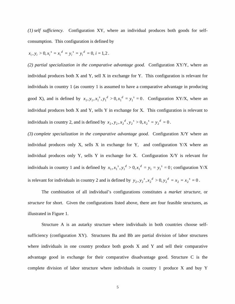
(1) self sufficiency. Configuration XY, where an individual produces both goods for self-

consumption. This configuration is defined by

x y x x y y ii i is

id

is

id, , , ,> = = = = =0 0 1 2 .

(2) partial specialization in the comparative advantage good. Configuration XY/Y, where an

individual produces both X and Y, sell X in exchange for Y. This configuration is relevant for

individuals in country 1 (as country 1 is assumed to have a comparative advantage in producing

good X), and is defined by x y x y x ys d d s1 1 1 1 1 10 0, , , ,> = = . Configuration XY/X, where an

individual produces both X and Y, sells Y in exchange for X. This configuration is relevant to

individuals in country 2, and is defined by x y x y x yd s s d2 2 2 2 2 20 0, , , ,> = = .

(3) complete specialization in the comparative advantage good. Configuration X/Y where an

individual produces only X, sells X in exchange for Y, and configuration Y/X where an

individual produces only Y, sells Y in exchange for X. Configuration X/Y is relevant for

individuals in country 1 and is defined by x x y x y ys d d s1 1 1 1 1 10 0, , ,> = = = ; configuration Y/X

is relevant for individuals in country 2 and is defined by y y x y x xs d d s2 2 2 2 2 20 0, , ,> = = = .

The combination of all individual’s configurations constitutes a market structure, or

structure for short. Given the configurations listed above, there are four feasible structures, as

illustrated in Figure 1.

Structure A is an autarky structure where individuals in both countries choose self-

sufficiency (configuration XY). Structures Ba and Bb are partial division of labor structures

where individuals in one country produce both goods X and Y and sell their comparative

advantage good in exchange for their comparative disadvantage good. Structure C is the

complete division of labor structure where individuals in country 1 produce X and buy Y

6

(configuration X/Y), and individuals in country 2 produce Y and buy X (configuration Y/X). It

can be shown that structures in which some countries export comparative disadvantage goods

cannot occur in general equilibrium.

Figure 1. Configurations and Structures

2.2. General equilibrium and its comparative statics

In a general equilibrium of the world each individual maximizes utility at a given set of

prices with respect to different configurations and quantities of production, trade, and

consumption and the set of prices clears the market.

The individuals make their utility maximization decisions based on the infra-marginal

analysis. The infra-marginal analysis is that for each configuration, individuals apply marginal

analysis to solve for the optimum quantities of consumption, production and trade, and then

apply total cost-benefit analysis to compare their utility across all configurations and choose the

configuration that gives the highest utility5.

5 The essence of the infra-marginal approach can be found in Coase (1946, 1960). Coase (1946) noted “a consumerdoes not only have to decide whether to consume additional units of a product; he has also to decide whether it isworth his while to consume the product at all rather than spend his money in some other direction” (p.173).Buchanan and Stubblebine (1962) introduced the concept of infra-marginal externality which is an early applicationof the infra-marginal analysis in welfare economics. Formally, the infra-marginal analysis is associated with non-linear or linear programming, while marginal analysis is associated with classical mathematical programming. Otherapplications of the infra-marginal analysis can be found in Arrow, Ng, and Yang (1998), Becker (1981), Dixit (1987,1989), Grossman and Hart (1986), Rosen (1983), and Yang and Y-K. Ng (1993).

Country 1 Country 2 Country 1 Country 1 Country 1 Country 2Country 2 Country 2

XY XY

Structure A Structure Ba Structure Bb Structure C

XY/Y XY/X X/Y Y/XX/YY/X

X

Y Y Y

X X

7

Since the individuals’ choice variables ( x x x y y yi is

id

i is

id, , , , , ) are not continuous across

configurations, we introduce the concept of corner equilibrium which is defined as a relative

price of the two goods and a resource allocation that satisfy (1) for a given structure (which is a

combination of all individuals’ configurations), each individual maximizes utility at a given

relative price, and (2) the relative price clears the market.

The general equilibrium is solved in two steps. First, we solve the corner equilibria for

each structure, then we identify the parameter subspace within which each corner equilibrium is

the general equilibrium where nobody has incentive to unilaterally deviate from his configuration

in this structure.

The corner equilibrium for each structure is solved by first solving the individuals’

decision problems to obtain the supply and demand functions for goods X and Y, and then using

the market clearing condition to find the corner equilibrium price. For instance, in Structure Ba,

the decision problem for individuals in country 1 is :

1

.s.t

)(max

11

11

111

1111

11111

,1,1,11,1 1

=+

=

=

=+

+= −

yx

sd

yy

xxs

d

lxldyysxx

ll

xpy

lay

laxx

kyyxUy

ββ

The first order conditions imply:

p = a1y/ka1x, x1 = βa1x, x1s = a1x(l1x-β), y1 = a1y(1-l1x), y1

d = a1y(l1x-β)/k,

where p p px y≡ / is the price of X in terms of Y.

The decision problem for individuals in country 2 is :

8

x y y

d

sy

s d

d sU kx y

y y a

y p x

2 2 22 2 2

1

2 2 2

2 2

,max ( )

.

=

+ =

=

−β β

s.t

The first order conditions imply:

xka a

a

y a

y a

d y x

y

y

sy

22 1

1

2 2

2 2

1

=

= −

=

β

β

β

( )

From the market clearing condition M x M xs d1 1 2 2= , we obtain:

l M ka M ax y y1 2 2 1 1= +( ) / ,β β which is less than 1 if and only if a2y/a1y<M1(1-β)/kM2β. That is,

Structure Ba is chosen only if a2y/a1y<M1(1-β)/kM2β.

The corner equilibria for Structure A, Bb and C are solved using the same approach as

above. The results are summarized in Table 1.

Table 1: Corner equilibria

Structure Price( / )p px y

Relevant ParameterSubspace

Individual Utility

Country 1 Country 2A N.A. U1(A)≡(βa1x)

β

[(1-β)a1y]1-β

U2(A)≡(βa2x)β

[(1-β)a2y]1-β

Ba a1y/ka1x k < k1 ≡ M1a1y(1-β)/βM2a2y< 1

U A1( ) U2(A)(k2a2ya1x/a2xa1y)

β

Bb ka2y/a2x k < k2 ≡ M2a2xβ/(1-β)M1a1x <1

U1(A)(k2a2ya1x/a2xa1y)

1-βU A2 ( )

C βM2a2y

÷M1a1x(1-β)U1(A)[βkM2a2y

÷M1a1y(1-β)]1-βU2(A)[(1-β)kM1a1x

÷M2a2x β]β

9

Now, we apply the definition of general equilibrium to find out under what conditions

each of the structures listed in table 1 occurs in general equilibrium.6 Consider structure Ba first.

Structure Ba is the general equilibrium structure if the following three conditions hold. First,

under the corner equilibrium relative price in this structure p = a1y/ka1x, individuals in country 2

prefer specialization in Y (configuration Y/X) to the alternatives, namely autarky (configuration

A) and specialization in X (configuration X/Y). In other words, the following conditions hold:

(1a) U2(Y/X) ≥ U2(A) which holds iff k≥k0≡[(a2x/a2y)/(a1x/a1y)]0.5,

(1b) U2(Y/X) ≥ U2(X/Y) which holds iff k≥k3≡[(a2x/a2y)/(a1x/a1y)]0.5/β.

Second, general equilibrium requires that all individuals in country 1 prefer configuration XY/Y

to the alternatives, that is,

(2a) U1(XY/Y) ≥ U1(X/Y) which holds iff a1y/a1x ≥ kp = a1y/a1x,

(2b) U1(XY/Y) ≥ U1(Y/X) which holds iff 1 ≥ k.

Third, no individual in country 1 is completely specialized in X, i.e.,

(3) l1x < 1, which holds iff k<k1≡a1yM1(1-β)/a2yM2β.

As k3≥k0, it follows that conditions (1)-(3) hold if k∈(k0, k1). Since k0< k1 holds iff M1(1-β)/M2β

> [(a2xa2y)/(a1xa1y)]0.5, the corner equilibrium in structure Ba is the general equilibrium if k∈(k0,

k1) and M1(1-β)/M2β > [(a2xa2y)/(a1xa1y)]0.5, where k1 ≡ a1yM1(1-β)/a2yM2β.

Similarly, we can identify the conditions for other structures to occur in general

equilibrium. These conditions are summarized in Table 2.

6 It can be shown that in a structure where the countries export their comparative disadvantage good individuals haveincentive to deviate from their configurations in this structure.

10

Table 2 General equilibrium

Parameter k k< 0 k k> 0

Subspaces M

M

a a

a ax y

x y

1

2

2 2

1 1

1

2

1>

−( )

ββ

M

M

a a

a ax y

x y

1

2

2 2

1 1

1

2

1<

−( )

ββ

k k k∈( , )0 1 k k∈( , )1 1 k k k∈( , )0 2 k k∈( , )2 1

GeneralEquilibriumStructure

A Ba C Bb C

where ka a

a ay x

y x0

1 2

2 1

1

2≡ ( ) , kM a

M ay

y1

1 1

2 2

1≡

−( )β

β, k

M a

M ax

x2

2 2

1 1 1≡

−β

β( )

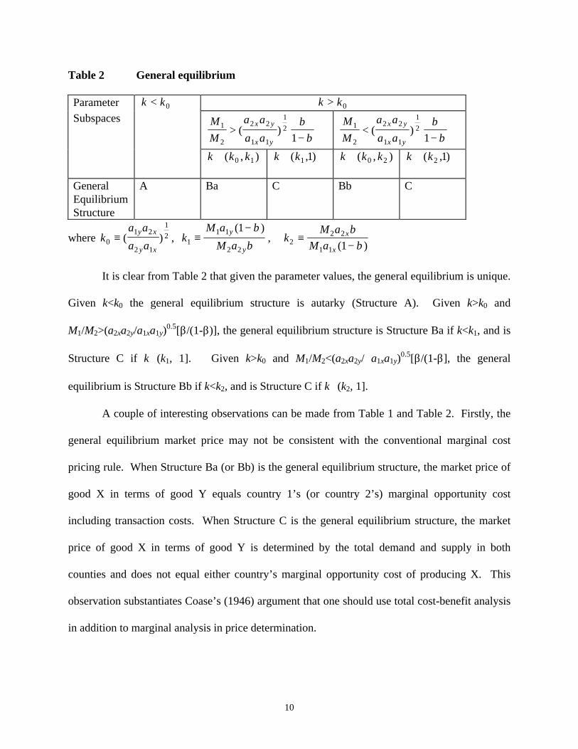
It is clear from Table 2 that given the parameter values, the general equilibrium is unique.

Given k<k0 the general equilibrium structure is autarky (Structure A). Given k>k0 and

M1/M2>(a2xa2y/a1xa1y)0.5[β/(1-β)], the general equilibrium structure is Structure Ba if k<k1, and is

Structure C if k∈(k1, 1]. Given k>k0 and M1/M2<(a2xa2y/ a1xa1y)0.5[β/(1-β], the general

equilibrium is Structure Bb if k<k2, and is Structure C if k∈(k2, 1].

A couple of interesting observations can be made from Table 1 and Table 2. Firstly, the

general equilibrium market price may not be consistent with the conventional marginal cost

pricing rule. When Structure Ba (or Bb) is the general equilibrium structure, the market price of

good X in terms of good Y equals country 1’s (or country 2’s) marginal opportunity cost

including transaction costs. When Structure C is the general equilibrium structure, the market

price of good X in terms of good Y is determined by the total demand and supply in both

counties and does not equal either country’s marginal opportunity cost of producing X. This

observation substantiates Coase’s (1946) argument that one should use total cost-benefit analysis

in addition to marginal analysis in price determination.

11

Secondly, we notice that under certain conditions, only when both countries have

absolute advantage in their comparative advantage goods, can Structure C be the general

equilibrium structure. For instance, if [ ( )] / ( )M M1 21 1− =β β (which holds if, but not only if,

both countries are of similar size and consumers’ preference for both goods are similar), we have

k a ay y1 1 2= / . Since k ∈( , )0 1 , k k> 1 can be satisfied only if a ay y2 1> . As k1 is relevant within

the parameter subspace, M1/M2>(a2xa2y/a1xa1y)0.5[β/(1-β)], which becomes

( ) / ( )a a a ax y x y2 2 1 1 1< when[ ( )] / ( )M M1 21 1− =β β . For k k> 1 to hold within this parameter

subspace, it is necessary that a ax x1 2> . Therefore, if [ ( )] / ( )M M1 21 1− =β β and

( ) / ( )a a a ax y x y2 2 1 1 1< , complete division of labor can occur in general equilibrium only if both

countries have absolute advantage in their comparative advantage good. A similar result can be

found in Chipman (1965, 1979) although his models did not incorporate positive transaction

costs.

We can conduct two types of comparative static analyses of the general equilibrium. The

first type is the conventional comparative static analysis for a given structure – the equilibrium

price, quantities of goods and the numbers of individuals selling different goods change

continuously in response to a continuous change in parameters.

The second type of comparative static analysis examines how changes in parameters

generate shifts of the general equilibrium across corner equilibria. It shows that the general

equilibrium price, quantities and indirect utility functions can discontinuously jump between

corner equilibria as parameters reach some critical values. Suppose the general equilibrium is

initially at Structure A, as the transaction efficiency coefficient (k) increases from a low value to

k0, and then to k1 or k2, the general equilibrium jumps from autarky to partial division of labor,

12

and then to complete division of labor. Whether the transitional structure is Ba or Bb depends on

the relative size and relative productivity of the two countries, and individuals’ relative

preference over the two goods. For instance, if country 1 is relatively large in size (large

M M1 2/ ), its relative productivity is high (large a a a ax y x y1 1 2 2/ ), and the consumer’s relative

preference is in favor of its comparative disadvantage good Y (large ( ) /1− β β ), then country 1

is likely to produce both goods X and Y, and the general equilibrium structure will be structure

Ba. As the general equilibrium pattern of division of labor changes, the equilibrium price also

changes discontinuously, so do individuals’ utility levels. Note that all critical values of k that

demarcate different structures are functions of relative population size, relative tastes, and

relative production condition. For instance, k0 is a decreasing function of the degree of

comparative advantage (a1x/a1y)/(a2x/a2y), k1 is a decreasing function of relative taste β/(1-β) and

an increasing function of relative population size, M1/M2, and the relative productivity of good y,

a1y/a2y. Hence, the inframarginal comparative statics of general equilibrium completely partition

the eight-dimension (β, a1x, a1y, a2x, a2y, M1, M2, k) parameter space into subspaces within which

particular corner equilibria are general equilibria. They rigorously identify the degree of

substitution between the parameters representing transaction conditions, production conditions,

and tastes for a shift of the general equilibrium from a structure to another. For instance, for a

given degree of comparative advantage, a sufficiently great increase in transaction efficiency will

generate a jump of the general equilibrium from autarky to the partial division of labor; while for

a given transaction efficiency, a sufficiently great increase in the degree of comparative

advantage will shift the general equilibrium from autarky to the partial division of labor too. In

this sense, our inframarginal comparative statics are much more than the statement that a better

13

transaction condition will generate a higher level of division of labor, which sounds like

tautology.

From the above analysis, we conclude:

Proposition 1 The general equilibrium structure is determined by the level of transaction

efficiency, the relative productivity and relative population size of the two countries, and

individuals’ relative preference over the two goods. Given other parameters, improvements in

transaction efficiency can make the general equilibrium structure jump from autarky to partial

division of labor and then to complete division of labor.

Proposition 1 implies that transaction efficiency plays an important role in determining

the size of the market, and the size of the market in turn determines the equilibrium pattern and

level of the division of labor. Thus, we have formalized Smith’s (1776) conjecture that the

division of labor is limited by the extent of the market, and the extent of the market is determined

by transportation costs.

It is interesting to note that in our model, an increase in transaction efficiency coefficient

(k) can increase total transaction costs because the increase in k can generate a jump of the

general equilibrium from a low level of division of labor to a higher level, thus increasing the

total number of transactions. This implication can be used to explain why the income share of

transaction costs has increased as transaction efficiency improves (North, 1986).

3. A 2x2 Ricardian model with tariff

Based on the model in section 2, suppose that country i (i = 1, 2) imposes an ad valorem

tariff of rate ti, and transfer all tariff revenue equally to all individuals in country i. In the case,

individuals’ budget constraint changes, for instance in configuration X/Y, from pxxs = pyy

d to pxx

s

14

+ r = (1+t)pyyd where r is transfer of tariff revenue from the government to an individual.

Individuals take the amount of transfer as given. At equilibrium, the amount of transfer equals

tariff revenue. Also, we assume that the transaction efficiency coefficient for country i is ki,

which may be different between countries. Using the same procedure as in section 2, we can

solve for the corner equilibrium for each structure. The corner equilibrium solutions are

presented in Table 3.

It is easy to see that if t1= t2=0 and k1= k2, Table 3 reduces to Table 1. If t1= t2=0, the

textbook Ricardian model predicts that the “large” country which produces both goods does not

get any gains from trade. This result can be clearly seen from Table 1 -- when the general

equilibrium occurs in structure Ba (or Bb), individuals in country 1 (or country 2) which

produces both goods X and Y get the same level of utility as they do in autarky.

Table 3: Corner equilibrium solutions

Structure Price( / )p px y

RelevantParameterSubspace

Individual Utility

Country 1 Country 2A N.A.

( )( ) [( ) ]β ββ βa a

U A

x y1 11

1

1−

≡

−

( )( ) [( ) ]β ββ βa a

U A

x y2 21

2

1 −

≡

−

Ba ( )

/

1 1

1 1 1

+ t

a k ay x

k M M

a a Dy y

1 1 2

1 2 1

1

<−

( / )

[( ) / ]

( / )

β β ( )AU

ttL x

1

111 )]1/()1[( β++

( )[ ( ) / ( )]k k a a a a

T U A

x y y x1 2 1 2 1 2

1 2

β

β

Bb k a

a t

y

x

2 2

2 21

/

[ ( )]+

k M M

a a Dx x

2 2 1

2 1 2

1

<−

( / )

[ / ( )]

( / )

β β ( )AUT

aaaakk xyyx

11

2

1212121 )]/()([

β

β

−

−

( )AUtt

Ltt x

222

222

)]1(

/)1[(

β−+−+

C ( / )

[ / ( )]

( / )

[( ) /

( ( ) ]

M M

a a

t

t

y x

2 1

2 1

1

2

1

1

1 1

β β

ββ

−

++ −

{( / )

[ / ( )]

( / )} ( )

k M M

a a T U Ay y

1 2 1

2 11

31

1

1β ββ β

−− −

{( / )

[( ) / ]

( / )} ( )

k M M

a a T U Ax x

2 1 2

1 2 4 2

1 − β ββ β

15

where D t t t1 1 2 11 1 1 1≡ + + − +( )[ ( ) ] / ( )β βD t t t2 1 2 21 1 1 1≡ + + + −( )( ] / [( ( ) )β β

βββββ >−++++= ]}1)[1/[()1){(/)(/( 2211121211 ttttaakMML yyx

T t t t t t t1 1 2 21

2 2 211 1 1 1≡ + + − + + −− −[( )( )] [( ) / ( )]( )/β β β β

βββββ <++−+−−= )}1)(1/[()1]{(/)1()[/( 2122122212 ttttaakMML xxx

T t t t t2 2 11

1 111 1 1 1≡ + + + +− −[( )( )] [( ) / ( )] /( )β β β β

T t t t t3 2 21

1 111 1 1≡ + − + +− −( ) [( ) / ( )] /( )β β β β

T t t t t4 11

2 2 211 1 1≡ + + + −− −( ) [( ) / ( )]( )/β β β β

The story is different when tariff is introduced. Refer to Table 3, if the general

equilibrium occurs in Structure Ba (or Bb), individuals in the country producing both goods, gets

a higher utility than they do in Autarky. Moreover, in Structure Ba, ∂U1/∂t1>0 (or in Structure

Bb, ∂U2/∂t2>0), that is, given the tariff rate of the country producing one good, the country

producing two goods can improve its own welfare by raising its tariff rate. This is because the

latter country determines the terms of trade, and it can improve its terms of trade by imposing a

tariff, thereby obtaining a larger share of the gains from trade. The gain of the country producing

two goods is at the expense of its trading partner as can be shown that ∂U2/∂t1<0 in Structure Ba

and ∂U1/∂t2<0 in Structure Bb. If the country producing two goods imposes a sufficiently high

tariff, the other country may want to withdraw from trade, in which case both countries are hurt.

In contrast to the country producing two goods, the completely specialized country has no

influence on the term of trade. As a result, it only hurts itself by imposing a tariff, as can be

derived from Table 3, ∂U2/∂t2<0 in Structure Ba and ∂U1/∂t1<0 in Structure Bb.

If both countries can influence the terms of trade (as in Structure C), then the gains of

trade are shared between the two countries. However, since ∂U1/∂t1 > 0 and ∂U2/∂t2 > 0 in

structure C, i.e., each country can benefit from raising its own tariff given the other country’s

tariff rate, each country will be tempted to raise its own tariff as much as possible. But if they

16

both raise tariff, both can be worse off. It can be shown that in Structure C ∂U1/∂t2<0 and

∂U2/∂t1<0, and that U1 converges to 0 as t2 tends to infinity and U2 converges to 0 as t1 tends to

infinity. This implies that as a country sufficiently increases its tariff, the other country will not

only be marginally worse off, but also discontinuously (inframarginally) jump from trade to

autarky.

The above analysis is conducted within the Walrasian regime. To analyze the behavior of

the governments in the two countries, we examine two other regimes: a Nash game and a Nash

tariff bargaining game.

First suppose the governments in the two countries play a Nash game. Each government

chooses its own tariff rate to maximize home resident’s utility, taking as given the tariff rate in

the foreign country and the Walrasian decisions of all individuals. For each structure (A, Ba, Bb

or C), a Nash corner equilibrium can be calculated. The Nash general equilibrium is one of four

Nash corner equilibria. Consider structure Ba first. Since ∂U2/∂t2<0 in this structure, the

equilibrium strategy of country 2’s government is to impose zero tariff. Since ∂U1/∂t1>0 and

∂U2/∂t1<0, the equilibrium strategy of country 1’s government is to impose a tariff as high as

possible provided each individual in country 2 will not deviate from configuration Y/X. If the

Nash corner equilibrium in structure Ba is the Nash general equilibrium, each individual in

country 2 is slightly better off than in autarky and most gains from trade go to country 1. In other

words, the Nash corner equilibrium in the tariff game in this structure generates a distribution

pattern of gains from trade that is opposite to the distribution in the absence of a tariff where all

the gains go to country 2.

This Nash corner equilibrium is not Pareto optimal because of the deadweight loss caused

by tariff. But the distortion caused by the tariff converges to zero as gains from trade net of

17

transaction costs go to zero. If each government can choose any level of tariff (including zero

tariff), the Walrasian equilibrium with no tariff will not occur when structure Ba is chosen in

general equilibrium because country 1’s government has an incentive to deviate from that

equilibrium by increasing tariff.

Since structure Bb is symmetric to Ba, we can obtain a similar result: a tariff game will

reverse the distribution pattern of gains from trade and generate distortions.

Now consider structure C. Since ∂U1/∂t1>0, ∂U2/∂t1<0, ∂U1/∂t2<0, ∂U2/∂t2>0 in this

structure, the Nash corner equilibrium strategy of each government in this structure is to impose a

tariff as high as possible provided the individuals in the other country will not deviate from their

configurations in this structure. This implies that the gains from the complete division of labor in

this structure will be almost exhausted by the deadweight loss caused by the tariff war. If the

Nash general equilibrium occurs in this structure, this equilibrium may generate very significant

welfare loss to both countries. This is a typical prisoners’ dilemma.

Now suppose the two governments play a Nash tariff bargaining game. This game

maximizes a Nash product of the net gains of the two countries with respect to tariff rates of the

two countries. Each country’s net gain is the difference between each individual’s realized utility

and her utility at a disagreement point. The Nash tariff negotiation equilibrium can be solved in

two steps: (1) a restricted Nash bargaining equilibrium is solved for a given structure, taking

another structure as a disagreement point; (2) the two governments bargain over choice of

structure.

The Nash product in structure C is

V = V1V2 = [U1(C)- U1(A)] [U2(C)- U2(A)]

18

where Ui(C) and Ui(A) are given in Table 3. The Nash bargaining corner equilibrium in structure

C is given by maximizing V with respect to t1 and t2. The two first order conditions ∂V/∂t1 =

∂V/∂t2 = 0 generate (1+t1)(1+t2) = 1. Hence, the solution of the Nash tariff negotiation game is t1*

= t2* = 0. This implies that the Nash tariff negotiation will generate a bilateral laissez faire

regime. But this laissez faire regime cannot be achieved in the absence of tariff negotiation

because of prisoners’ dilemma.

Although in this Nash bargaining game, no risk is specified, the players’ attitude towards

risk “plays a central role” (Osborne and Rubinstein, 1990, p.10). As long as there exists

uncertainty about other players’ behavior, there is chance that the negotiation breaks down.

Thus each player intends to maximize her expected utility gain in the negotiation. In fact, the

Nash product can be interpreted as a player’s expected utility gain, with the probability of

reaching an agreement being approximated by the utility gain(s) of the other player(s).

According to this view of Nash (1950), the Nash bargaining solution is the outcome of a non-

cooperative game despite the fact that the gains are shared fairly among players.

If each government can decide whether or not to participate in a tariff negotiation game,

then it is clear that when structure Ba or Bb occurs in general equilibrium, it must be a Nash

equilibrium with no tariff negotiation since the country producing two goods can get most of the

gains from unilateral tariff. When structure C occurs in general equilibrium, the general

equilibrium must involve tariff negotiation since both governments prefer tariff negotiation to

tariff war -- clearly, the two countries receive more net gains in the tariff negotiation game than

in the tariff war since the Nash tariff bargaining equilibrium, which coincides with the Walrasian

equilibrium with not tariff, is Pareto optimal.

19

This result explains why it is difficult to realize laissez faire regimen even if it is good for

all countries. When sovereignty of a country can be used to seek rent in international trade via

taxation power, coordination difficulty in a prisoners’ dilemma makes tariff negotiation essential

for fully exploiting mutually beneficial gains from trade. Following the method in the previous

section, we can show that in the model with endogenous choice of regimes, the general

equilibrium discontinuously jumps from autarky to structure Ba or Ba, then to structure C as the

transaction efficiency coefficient k increases.

Summarizing the above analysis, we have:

Proposition 2 In a model with the two governments which can choose tariff level and decide

whether or not to participate in tariff negotiations, if partial division of labor occurs in

equilibrium, it is a Nash tariff equilibrium with no tariff negotiation. Most gains from trade go to

the country producing both goods. If complete division of labor occurs in equilibrium, it is a

Nash tariff negotiation equilibrium which generates bilateral laissez faire regime.

Proposition 2 may be used to explain two phenomena. First, despite the distortions

caused by tariff, tariff may be used by a government to get a larger share of gains from trade

since the Walrasian equilibrium with no tariff may divide gains to trade very unequally between

countries. Second, when transaction condition is not very good so that the equilibrium is

associated with an intermediate level of division of labor, some countries (which do not

completely specialize) may prefer a unilateral tariff, whereas other countries (which completely

specialize) may prefer a unilateral laissez faire regime. But as transaction conditions improve, all

countries may prefer tariff negotiations to a unilateral tariff or a unilateral laissez faire regime.

In the 16th and 17th century, unilateral tariff was advocated by Mercantilists as a means of

rent seeking in international trade (see for instance Ekelund and Tollison, 1981). It gave way to

20

trade liberalization in the 18th and 19th century in some European countries. However, even after

World War II, many governments in developing countries still adopted unilateral tariff

protection. More recently, tariff negotiations have become increasingly prevalent. Some

economists use the Walrasian model to explain the emergence of laissez faire regime, but the

model cannot explain why other trade regimes persisted in many countries for a long period of

time. Other economists use the theory of import substitution and export substitution to explain

the transition from unilateral tariff to trade liberalization (see, for instance, Balassa, 1980 and

Bruton, 1998), but the theory cannot explain why laissez faire regime was unstable even between

developed countries; why some countries prefer unilateral protection tariff and others prefer

laissez faire regime; and why tariff negotiations may be necessary for the exploitation of the

gains from trade. Proposition 2 in this paper seems to offer a more plausible explanation as to

why unilateral tariff prevailed in the early stage of economic development; why trade

liberalization is preferred in later stages of economic development; why unilateral tariff and

unilateral laissez faire regime coexist, and under what condition tariff negotiation is essential for

the exploitation of gains from trade.

4. A 3x2 Ricardian Model

In this section, we extend the simple 2x2 Ricardian model to include a third country,

country 3. It is assumed that transaction conditions are different from country to country such

that k1, k3 > k2, where ki is the transaction efficiency coefficient in country i. We intend to show

that a country which does not have a comparative advantage to the other two countries and/or

which has low transaction efficiency can be excluded from trade.

21

Suppose that the production functions in country i (i = 1, 2, 3) are the same as in

subsection 2.1 and that (a3x/a3y) < (a2x/a2y) < (a1x/a1y), i.e., country 1 has a comparative advantage

in producing good X to the other two countries, country 2 has a comparative advantage in

producing X relative to country 3, and a comparative advantage in producing good Y relative to

country 1; and country 3 has a comparative advantage in producing Y to the other two countries.

We consider only the case where the trading countries are completely specialized. For

similar reasons discussed in subsection 2.2, all structures involving trade in comparative

disadvantage goods cannot occur in general equilibrium. We now prove that if a structure which

involves trading between only two of the three countries, the two trading countries must be

country 1 and country 3. In other words, the country which has the lowest transaction efficiency

and/or has no comparative advantage to the other two countries may be excluded from trade.

Suppose only country 1 and country 2 trade. This can occur in general equilibrium only if

individuals in country 2 prefer specialization in Y (or configuration Y/X) to autarky and

individuals in country 3 prefer autarky to specialization in Y. That is, the following inequalities

hold:

U2(Y/X) > U2(A) which holds iff p<(a2y/a2x)k2 and

U3(Y/X) < U3(A) which holds iff p>(a3y/a3x)k3.

where the indirect utility functions for different configurations are from Table 1. The two

inequalities jointly imply (a2x/a2yk2)<(a3x/a3yk3) which contradicts the assumption

(a2x/a2y)>(a3x/a3y) and k2 < k3.

Suppose instead only country 2 and country 3 trade. This can occur in general

equilibrium only if

U2(X/Y) > U2(A) which holds iff p>a2y/a2xk2 and

22

U1(X/Y) < U1(A) which holds iff p<a1y/a1xk1.

The two inequalities jointly imply (a1y/a1xk1)>(a2y/a2xk2) which contradicts the assumption

(a1x/a1y)>(a2x/a2y) and k2 < k1.

Next we examine the conditions under which the structure involving trade between only

country 1 and country 3 occurs in general equilibrium. The conditions are:

U1(X/Y) > U1(Y/X) which holds iff p>(a1y/a1x)k12β-1,

U1(X/Y) > U1(A) which holds iff p>a1y/a1xk1,

U2(X/Y) < U2(A) which holds iff p<a2y/a2xk2,

U2(Y/X) < U2(A) which holds iff p>(a2y/a2x)k2,

U3(Y/X) > U3(A) which holds iff p<(a3y/a3x)k3,

U3(Y/X) > U3(X/Y) which holds iff p<(a3y/a3x)k32β-1,

where p = a3yM3β/a1xM1(1-β) is the corner equilibrium relative price in this structure.

The six inequalities together imply Min{a2y/a2xk2, (a3y/a3x)k3}> a3yM3β/a1xM1(1-β) >

Max{a1y/a1xk1, (a2y/a2x)k2}. The parameter subspace satisfying this condition is certainly not

empty. For instance, if k2 is sufficiently close to 0 and k1 and k3 are sufficiently close to 1, then

the above condition becomes (a3y/a3x)k3> a3yM3β/a1xM1(1-β) > a1y/a1xk1, or (a1x/a3x)k3 >

M3β/M1(1-β) > a1y/a3yk1, which holds only if k3k1[(a1x/a1y)/(a3x/a3y)] > 1. This condition can be

satisfied if the relative population size is not too far away from a balance with relative tastes, the

two countries’ transaction conditions are sufficiently good and the degree of comparative

advantage (measured by (a1x/a1y)/(a3x/a3y) ) between the two countries is great.

23

Summarizing the above analysis, we obtain:

Proposition 3 In a 3x2 Ricardian model within certain parameter subspace, it is possible that

the country that has no comparative advantage in producing any good over both of its potential

trading partners and/or that has very low transaction efficiency will be excluded from trade.

This proposition can accommodate opinions of both sides in a recent debate on

international competitiveness. Krugman (1994) argued that a nation should focus on promoting

free trade and that the emphasis on international competitiveness can be “a dangerous

obsession”. Sachs (1996) and Prestowitz et. al. (1994), on the other hand, contended that

international competitiveness plays an essential role in improving national welfare. If

international competitiveness is measured by a country’s transaction efficiency, then proposition

3 confirms that competitiveness matters. Proposition 3 implies that comparative advantage is not

enough for realizing gains from trade. A country can be excluded from trade even if it has

comparative advantage to another single country when its transaction efficiency is low or/and it

has no comparative advantage to both of the other potential partners. However, the proposition

also supports Krugman’s argument that a country should focus on promoting free trade and

improving transaction efficiency. In our model, the promotion of free trade can be done through

reducing tariff and non-tariff barriers of trade so as to improve transaction efficiency k. If k is

extremely low ( k k< 0), no trade occurs and absolute and comparative advantage does not do

good for trade. Since in our model the improvement of the transaction efficiency coefficient

through trade liberalization policies can generate a jump of general equilibrium from a low to a

high level of division of labor, the argument for free trade is even stronger than the conventional

marginal analysis suggests. Therefore, international competitiveness and free trade are important

factors contributing to a country’s welfare. And Krugman’s emphasis on trade liberalization is

24

particularly relevant if the pursuit of international competitiveness is used as an excuse for

impeding free trade.

Introducing tariff into the model in this section, it can be shown that when all

governments are allowed to choose tariff level and tariff negotiation and when the partial

division of labor occurs in general equilibrium, the country with a higher tariff and/or worse

transaction condition (a small value of k) will be excluded from trade. Hence, in a world

economy with many governments, even in the partial division of labor, tariff rates will be

reduced by competition between the governments in those similar countries. Since a greater value

of k will increase the number of countries that are involved in international trade, which will in

turn ensure a multilateral free trade regime even if the partial division of labor occurs in general

equilibrium, a sufficiently great increase in k in the country that was excluded from trade can

then ensure a zero tariff rate for all countries even if the general equilibrium is associated with

the partial division of labor. This result implies that there are two possible explanations for a shift

of trade regime from protection tariff to trade liberalization. The first is to attribute such a shift to

the increase in the level of division of labor (a shift from the partial division of labor to the

complete division of labor), which is caused by improvements in transaction conditions. The

second is to attribute such a shift to the increase in the number of countries that are involved in

international trade, which is caused by improvements of the transaction conditions in those

countries which used to be excluded from trade. Since an increase in k can be generated either by

improvements in transportation conditions (the emergence of new transportation technology or

the development of transportation infrastructure) or by institutional changes (the emergence of a

legal system that more effectively protects property rights or a more competitive and efficient

25

banking system), we can explain this shift of trade regime by improvements of transportation and

institution environment.

5. Conclusion

In this paper, we have studied a general equilibrium 2x2 Ricardian model using the infra-

marginal analysis. Departing from the neoclassical paradigm where individuals’ levels of

specialization are not endogenized, we explain international trade by individuals’ choices of their

levels and patterns of specialization. In our analysis, the traditional rule of marginal cost pricing

may not be applicable; and the comparative statics involve discontinuous jumps -- as transaction

efficiency improves, the general equilibrium structure may jump from autarky to partial division

of labor and then to complete division of labor. This prediction is supported by historical

evidences documented in North (1958) and North and Weingast (1989) and by empirical

evidences provided in Barro (1997), Easton and Walker (1997), Frye and Shleifer (1997), Gallup

and Sachs (1998), Sachs and Warner (1995, 1997).

We have also examined some effects of tariff when the government can choose tariff

level and can decide whether or not to participate in tariff negotiations. If the partial division of

labor occurs in equilibrium, then the general equilibrium is associated with unilateral tariff by the

country producing both goods and most gains from trade go to this country, while the completely

specialized country chooses unilateral laissez faire regime. If the complete division of labor

occurs in equilibrium, the equilibrium regime is tariff negotiation which generates bilateral

laissez faire regime and fairly divides gains to trade between the two countries. Tariff

negotiation is essential for realizing free trade.

26

Finally, we have shown that in a 3x2 model the country that does not have a comparative

advantage over both of the other countries and/or that has low transaction efficiency may be

excluded from trade.

A logical extension of this paper is to incorporate fixed learning costs and other types of

increasing returns to specialization to the Ricardian model. The economies of specialization will

generate endogenous comparative advantage (Yang, 1994). It will be interesting to see how

exogenous and endogenous comparative advantage interact with each other and what

implications such interactions generate. Also, more goods and countries may be introduced into

our model to test robustness of our results.

27

References

Arrow, A., Y-K Ng, and X, Yang (1998), Increasing Returns and Economics Analysis, London: Macmillan.

Balassa, B. (1980), The Process of Industrial Development and Alternative Development Strategies, PrincetonUniversity, International Finance Section, Essays in International Finance, No. 141.

Barro, R. (1997), Determinants of Economic Growth, Cambridge, MA, MIT Press.

Becker, Gary (1981), A Treatise on the Family, Cambridge, Massachusetts, Harvard University Press.

Bruton, Henry (1998), “A Reconsideration of Import Substitution,” Journal of Economic Literature, 36, 903-36.

Buchanan, James M. and Stubblebine, W. Craig (1962), “Externality,” Economica, 29, 371-84.

Chipman, John (1965), “A Survey of the Theory of International Trade, Part 1, the Classical Theory,” Econometrica,33(3), 477-519.

Chipman, John (1979), “Mill’s ‘Superstructure’: How Well Does it Stand up?” History of Political Economy, 11(4),477-504.

Coase, Ronald (1946), “The Marginal Cost Controversy,” Economica, 13, 169-82.

Coase, Ronald (1960), “The Problem of Social Cost,” Journal of Law and Economics, 3, 1-44.

Dixit, A. (1987), "Trade and Insurance with Moral Hazard," Journal of International Economics, 23, 201-20.

Dixit, A. (1989), "Trade and Insurance with Adverse Selection," Review of Economic Studies, 56, 235-48.

Dixit, A. and Norman, V. (1980), Theory of International Trade, Cambridge: Cambridge University Press.

Dornbusch, Rudiger; Fischer, Stanley; Samuelson, Paul A. (1977), "Comparative Advantage, Trade, and Paymentsin a Ricardian Model with a Continuum of Goods." American Economic Review. 67, 823-39

.Ekelund, Robert, and Robert Tollison (1981), Merchantilism as an Rent-seeking Society, College Station, TX, Texas

A & M University Press.

Easton, Stephen and Michael, Walker (1997): "Income, Growth, and Economic Freedom", American EconomicReview, Papers and Proceedings, 87, 328-32.

Frye, Timothy and Shleifer, Andrei (1997): "The Invisible Hand and the Grabbing Hand.” American EconomicReview, Papers and Proceedings, 87, 354-58.

Gallup, John and Jeff Sachs (1998), “Geography and Economic Development,” Working Paper, Harvard Institute forInternational Development.

Gomory, Ralph E. (1994), “A Ricardo Model with Economies of Scale,” Journal of Economic Theory, 62, 394-419.

Grossman, S. and Hart. O (1986), “The Costs and Benefits of Ownership: A Theory of Vertical and LateralIntegration,” Journal of Political Economy, 94, 691-719.

Houthakker, H. S. (1976), “The Calculation of Bilateral Trade Patterns in a Ricardian Model with IntermediateProducts and Barriers to Trade,” Journal of International Economics, 6, 251-288.

28

Krugman, Paul (1994), “Europe Jobless, America Penniless?” Foreign Policy, 95, 19-34.

Krugman, Paul (1994), “Competitiveness: A Dangerous Obsession,” Foreign Affairs, 73(2), 28-44.

Nash, J. F. (1950), “The Bargaining Problem,” Econometrica, 18, 115-62.

North, D. (1958), "Ocean Freight Rates and Economic Development", Journal of Economic History, ??, 537-55.

North, D. (1986), "Measuring the Transaction Sector in the American Economy", in S. Eugerman and R. Gallman, eds.,.Long Term Trends in the American Economy, Chicago, University of Chicago Press.

Osborne, Martin J. and Rubinstein, Ariel (1990), Bargaining and Markets, San Diego: Academic Press, Inc.

Prestowitz, Clyde V. Jr et al. (1994), “The Fight over Competitiveness,” Foreign Affairs, 73(4), 186-197.

Ricardo, David (1817), The Principles of Political Economy and Taxation, London: J.M. Dent & Sons Ltd., 1965.

Rosen, S. (1978), “Substitution and the Division of Labor,” Economica, 45, 235-50.

Rosen, S. (1983), “Specialization and Human Capital,” Journal of Labor Economics, 1, 43-49.

Sachs, Jeffrey (1996), “The Tankers Are Turning - Sachs on Competitiveness,” World Link, September/October1996

Sachs, Jeffrey (1996), “On the Tigers Trail, - Sachs on Competitiveness,” World Link, November/December 1996.

Sachs, Jeffrey and Warner, Andrew (1997): "Fundamental Sources of Long-Run Growth.” American EconomicReview, Papers and Proceedings, 87, 184-88.

Smith, Adam (1776), An Inquiry into the Nature and Causes of the Wealth of Nations, reprint, Oxford: ClarendonPress, 1976.

Yang, Xiaokai (1994), “Endogenous vs. Exogenous Comparative Advantages and Economies of Specialization vs.Economies of Scale,” Journal of Economics, 60, 29-54.

Yang, Xiaokai and Ng, Yew-Kwang (1993), Specialization and Economic Organization, a New ClassicalMicroeconomic Framework, Amsterdam: North-Holland.

Yang, Xiaokai and Ng, Siang (1998), “Specialization and Division of Labor: A Survey,” in K. Arrow, Y-K Ng andX, Yang eds. Increasing returns and Economics Analysis, London: Macmillan.