city research onlineopenaccess.city.ac.uk/15825/1/chukanova, ekaterina.pdf · 6 figure 20:...

City, University of London Institutional Repository

Citation: Chukanova, E. (2016). Modelling of screw compressor plant operation under intermittent conditions. (Unpublished Doctoral thesis, City, University of London)

This is the accepted version of the paper.

This version of the publication may differ from the final published version.

Permanent repository link: http://openaccess.city.ac.uk/15825/

Link to published version:

Copyright and reuse: City Research Online aims to make research outputs of City, University of London available to a wider audience. Copyright and Moral Rights remain with the author(s) and/or copyright holders. URLs from City Research Online may be freely distributed and linked to.

City Research Online: http://openaccess.city.ac.uk/ [email protected]

City Research Online

http://openaccess.city.ac.uk/

mailto:[email protected]

MODELLING OF SCREW COMPRESSOR

PLANT OPERATION UNDER

INTERMITTENT CONDITIONS

by Ekaterina Chukanova

Thesis submitted for the

Degree of Doctor Philosophy

in Mechanical Engineering

City University London

December 2015

2

Contents

Contents ....................................................................................................................... 2

List of Figures .............................................................................................................. 5

List of Tables................................................................................................................ 9

Nomenclature ............................................................................................................. 10

Acknowledgments ...................................................................................................... 12

Abstract ...................................................................................................................... 13

1. Introduction ......................................................................................................... 14

1.1. Phenomena Associated with Transient Behaviour of Screw Compressors ........ 17

1.2. Thesis Outline ..................................................................................................... 17

2. Literature review .................................................................................................... 19

2.1. Transient behaviour and its effects ..................................................................... 19

2.1.1. Startup and Shutdown of Process Plant ........................................................ 19

2.1.2. Effects of Parameter Changes ...................................................................... 20

2.1.3. Control Systems Design ............................................................................... 20

2.2. Dynamic modelling ............................................................................................. 21

3. Aims of the Research and its Contribution to Science and Engineering ............... 23

3.1. Aims of the research............................................................................................ 23

3.2. Contribution to Science and Engineering ........................................................... 23

4. Experimental Studies ............................................................................................. 26

4.1. Test Rig Description ........................................................................................... 27

4.1.1. Oil-Injected Air Compressor Plant ............................................................... 27

4.1.2. Oil-Free Air Compressor Test Plant ............................................................. 29

5.1 Equations governing the screw compressor process ............................................ 32

5.2 The unsteady process in a lumped volume of the plant reservoirs and connecting

pipes ........................................................................................................................... 35

6. Startup Test Results and Data Analysis ................................................................. 39

3

6.1 Verification of Filling Tank Simulation ............................................................... 39

6.2. Data Analysis ...................................................................................................... 40

6.3. Torque Classification and Moment of Inertia Quantification ............................. 47

7. Screw Compressor Plant Model Validation ........................................................... 51

7.1. Oil-injected compressor ...................................................................................... 51

7.2. Oil-Free Compressor ........................................................................................... 56

8. Screw Compressor Plant Simulation Cases ........................................................... 59

8.1. The Effects of Plant Parameter Variation in Oil-Injected Air Screw Compressor

Systems on Response times and Final Steady Flow Conditions ................................ 59

8.1.1. Variation of Valve Area ............................................................................... 59

8.1.2. Varying the Tank Volume ............................................................................ 60

8.1.3. Varying the Tank Pressure ........................................................................... 62

8.2. Closed loop Screw Compressor Plant Simulations ............................................. 63

8.2.1. Varying the Compressor Shaft Speed in a Closed Loop System ................. 64

8.2.2. Variation of Shaft Speed during Compressor Operation in a Closed Loop

System .................................................................................................................... 65

8.3. Simulation of Multiple Tank Screw Compressor Plant ...................................... 68

8.3.1. Scenario 1: Time Variation .......................................................................... 68

8.3.2. Scenario 2: Valve Area Variation................................................................. 71

8.3.3. Scenario 3: Valve Area and Tank Volume Variation ................................... 73

8.3.4. Scenario 4: Four Tank Compressor Plant ..................................................... 76

8.3.5. Scenario 5: Simulation of a Plant where the Tanks are widely separated .... 79

8.4. Simulation of Steady and Intermittent Modes in order to Estimate Plant

Performance ............................................................................................................... 83

8.5. Pressure Range Limit Simulation ....................................................................... 86

9. Conclusions ............................................................................................................ 88

10. Recommendations for Future Work ..................................................................... 89

Bibliography ............................................................................................................... 90

4

Appendix 1. Screw Compressor Working Principle .................................................. 95

Appendix 2. Instrumentation and Instruments Calibration ........................................ 97

Appendix 3. Data Acquisition and processing ......................................................... 100

Appendix 4. Reynolds Transport Theorem .............................................................. 101

Appendix 5. Publications ......................................................................................... 105

5

List of Figures

Figure 1: Twin screw compressor .............................................................................. 14

Figure 2: Oil-injected process screw compressor plant, the compressor is on the

right, the oil-separator on the left, the suction pipe on the top and service ladders in

the middle (Courtesy of Howden. Compressors) ....................................................... 15

Figure 3: Laboratory Air Compressor Test Rig for both oil-free and oil-injected

machines ..................................................................................................................... 26

Figure 4: Schematic view of oil-injected compressor test rig – Computer screen..... 27

Figure 5: Oil-injected screw compressor tested ......................................................... 28

Figure 6: Schematic view of oil-free compressor test rig – Computer screen ........... 29

Figure 7: Tested oil-free machine .............................................................................. 30

Figure 8: Screw compressor plant model used for transient analysis ........................ 36

Figure 9: Flow Chart of transient screw compressor plant program .......................... 38

Figure 10: Measured and predicted rates of pressure rise in the tank during

compressor startup when the starting pressure is 5 bar .............................................. 39

Figure 11: Measured and predicted rates of pressure rise in the tank during

compressor startup when the starting pressure is 7 bar .............................................. 40

Figure 12: Oil-injected air compressor startup characteristics when discharging at

atmospheric pressure .................................................................................................. 41

Figure 13: Oil-injected air compressor startup at increased discharge pressure.

Decrease of torque between 1.7 and 2 s is due to the improved lubrication after the

oil flow was established ............................................................................................. 42

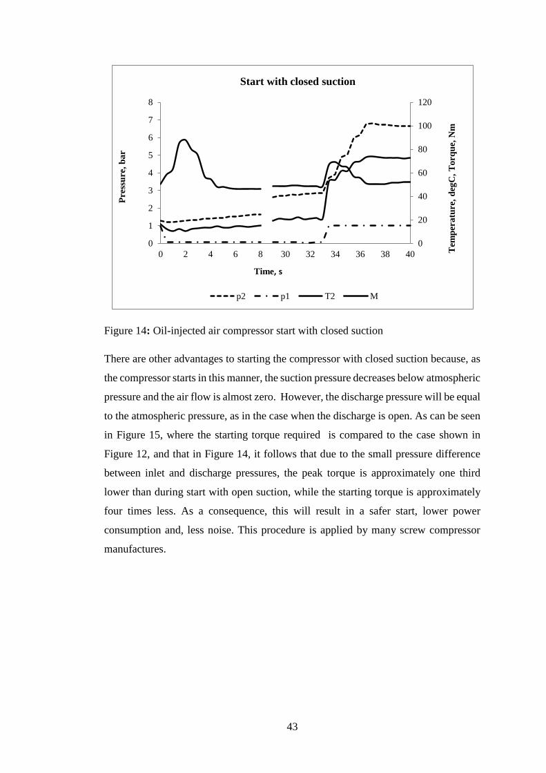
Figure 14: Oil-injected air compressor start with closed suction .............................. 43

Figure 15: Comparison of startup with open and closed suction for oil-injected air

compressor, Upper graph shows Torque, Lower graph shows discharge pressure ... 44

Figure 16: Startup times for oil-injected air compressor at different discharge

pressures, For clarity, the same starting point is assumed fo all cases...................... 45


pressures ..................................................................................................................... 46

Figure 18: Startup torque variation with discharge pressure for oil-injected air

compressor ................................................................................................................. 46

Figure 19: Discharge pressure curves for oil-injected air compressor startups at

different pressures ...................................................................................................... 47

6

Figure 20: Comparison between simulated and measured Speed and Torque changes

for oil-injected air compressor at a discharge pressure of 7 bar ................................ 48

Figure 21: Starting torque diagrams for an oil-injected air compressor discharging at

atmospheric pressure .................................................................................................. 49


above atmospheric pressure ....................................................................................... 49

Figure 23: Comparison of estimated and measured pressure changes in oil-injected

air screw compressor plant. Differences < 5% .......................................................... 51

Figure 24: Comparison of estimated and measured temperature changes in oil-

injected air screw compressor plant. Differences < 5% ............................................. 52

Figure 25: Comparison of estimated and measured mass flow rate changes in oil-


Figure 26: Comparison of estimated and measured input power changes in oil-


Figure 27: Comparison of estimated and measured pressure changes in oil-injected


Figure 28: Comparison of estimated and measured temperature changes in oil-




Figure 30: Comparison of estimated and measured input power changes in oil-


Figure 31: Comparison of estimated and measured pressure changes in oil free air

screw compressor plant. Differences < 5% ................................................................ 57

Figure 32: Comparison of estimated and measured temperature changes in oil free air


Figure 33: Comparison of estimated and measured mass flow changes in oil free air


Figure 34: Comparison of estimated and measured power input changes in oil free


Figure 35: The effect of varying the valve area in an oil-injected air screw

compressor plant. The upper graph shows the Tank Pressure, and the lower graph

shows the Temperature .............................................................................................. 60

7

Figure 36: The effect of varying the tank volume in an oil-injected air screw



Figure 37: The effect of varying the initial tank pressure in an oil-injected air screw



Figure 38: Two tank closed loop screw compressor plant system ............................. 63

Figure 39: Pressure variation in the discharge Tank, as a result of speed changes in a

closed loop air screw compressor plant ..................................................................... 64

Figure 40: Mass flow going to both tanks at different shaft speeds........................... 65

Figure 41: The effect of sudden speed variation on discharge pressure, when

changing speed from 3000 to 6000rpm ...................................................................... 66

Figure 42: The effect of sudden variation of speed from 3000 to 6000 rpm on the

Mass flow in and out .................................................................................................. 66

Figure 43: Change of mass of air in both tanks, as a result of changing speed from

3000 to 6000rpm ........................................................................................................ 67

Figure 44: Pressure changes in both tanks, resulting from speed changes from 3000

to 6000rpm and back to 3000. .................................................................................... 67

Figure 45: Compressor plant layout for multiple tank configuration ........................ 68

Figure 46: Pressure variation in Tank 2 and Tank 3 for different cycle time Intervals

.................................................................................................................................... 69

Figure 47: Temperature variation in Tank2 and Tank3 for different cycle time

intervals ...................................................................................................................... 70

Figure 48: Pressure in Tank2 and Tank3 and input power for cases 1-5 ................... 72

Figure 49: Compressor plant layout for multiple tank configuration ........................ 73

Figure 50: Rates of pressure change in Tank2 and Tank3 for varying valve areas and

tank capacities ............................................................................................................ 74

Figure 51: Rates of temperature change in Tank2 and Tank3 for varying valve areas

and tank capacities ..................................................................................................... 75

Figure 52: Four tank compressor plant configuration ................................................ 76

Figure 53: Pressure in the tank after compressor for 2-, 3- and 4-tank systems ........ 76

Figure 54: Variation of pressure, above, and temperature, below, in three tank

compressor plant model depending on speed changes ............................................... 77

8

Figure 55: Variation of pressure and temperature in a four tank compressor plant

model resulting from step changes in speed. ............................................................. 78

Figure 56: Screw compressor plant with widely spaced tanks .................................. 79

Figure 57: Rates of pressure and mass flow change in a widely spaced tank system 80

Figure 58: Moody diagram ........................................................................................ 81

Figure 59: Alternative screw compressor plant scheme ............................................ 82

Figure 60: Pressure variation in the tank resulting from sudden valve area changes 83

Figure 61: Valve area variation for steady and unsteady modes ............................... 84

Figure 62: Pressure in the system for steady and unsteady cases, example 1 ............ 84

Figure 63: Pressure variation in the system for steady and unsteady cases, example 2

.................................................................................................................................... 85

Figure 64: Pressure for simulated switch off and switch on ...................................... 86

Figure 65: Pressure curve for simulated switch repetitive on/off operation .............. 87

Figure 66: Multiple tank configuration for further modelling ................................... 89

Figure 67: Compression process inside of screw compressor ................................... 95

Figure 68: Torque meter calibration .......................................................................... 97

Figure 69: Torque meter calibration results ............................................................... 98

Figure 70: Hydraulic dead weight tester .................................................................... 98

9

List of Tables

Table 1: Types of screw compressor plant and their associated transient phenomena

.................................................................................................................................... 17

Table 2: Oil-injected compressor experimental plan: Initial pressure and speed values

are not highlighted. Experimentally obtained pressure values are highlighted in grey

.................................................................................................................................... 29

Table 3: Oil-free compressor experimental plan: Initial pressure and speed values are

not highlighted. The final obtained pressures are highlighted in grey ....................... 31

Table 4: Torque effects during oil-injected air compressor startup ........................... 50

Table 5: Scenarios plan .............................................................................................. 68

Table 6: Valve area variation cases ............................................................................ 71

Table 7: System parameter comparison, example 1................................................... 85

Table 8: System parameters comparison, example 2 ................................................. 85

Table 9: Initial parameters of the system ................................................................... 86

Table 10: Description of the test rig instruments ....................................................... 99

Table 11: Attended conferences ............................................................................... 105

10

Nomenclature

A – cross section area of control valve, [m2]

Ag – clearance gap cross-sectional area, [m2]

coil – specific heat, [J/kgK]

Dg – effective diameter of clearance gap, [m]

d – screw compressor rotor diameter, [m]

dh – pipe hydraulic diameter, [m]

fd – Darcy friction factor,

h – specific enthalpy, [J/kg]

L – length of the rotor, [m]

lg – leakage clearance length, [m]

M – torque, [Nm]

m – mass, [kg]

min –mass flow entering the tank, [kg/s]

mout –mass flow leaving the tank, [kg/s]

p0 – atmospheric pressure, [Pa]

p1 – pressure in the compressor tank, [Pa]

p2 – pressure in the tank at the next time step, [Pa]

��– heat transfer between fluid and compressor surroundings, [J]

R - gas constant, [J/molK]

Re – Reynolds number,

T2 - Temperature in the tank, [K]

Tin – temperature of the gas entering the tank, [K]

Tout – temperature of the gas leaving the tank, equal to T2, [K]

tfl – flow time, [s]

Δt – time step, [s]

U - internal energy, [J]

u - specific internal energy, [J/kg]

V – volume of the plant containing tank and pipes, [m3]

V – local volume of the compressor working chamber, [m3]

v – fluid velocity, [m/s]

w – suction/discharge port velocity, [m/s]

11

wl – leaking gas velocity, [m/s]

γ – isentropic gas constant

δg – leakage clearance width, [μm]

φ – angular coordinate,

φ – transported property in generic transport equation

– main rotor angle,

μ – flow coefficient,

ν – kinematic viscosity, [m2/s]

ρl – leaking gas density, [kg/m3]

ρ2 – density of the gas in the tank, [kg/m3]

ω – angular velocity, [rad/s].

12

Acknowledgments

I feel very honoured to be a student of Professor Stosic – a brilliant engineer, a great

teacher and a man with a big heart. Without his support, guidance and encouragement

my PhD thesis would have never been completed. His patience, knowledge and

enthusiasm have no limit.

I would also like to thank Professor Kovacevic, without whom this thesis had never

been started, who initially trusted to my ideas and continued guiding me through the

whole process of it.

Also, my very best gratitude to my colleagues for the continuous help and discussions

over the years: Dr Sham Rane, Dr Matthew Read, Dr Ashvin Dhunput, Ms Madhulika

Kethidi, Mr Mohammad Arjeneh. Special thanks to Mr Mike Smith for his help with

the test rig.

I want to thank company Howden where I got inspiration and ideas for my research

and people who supported me there: Mr Eric Schwab, Mr Peter Goddard, Mr Paul

Hendry and Mr Kirill Zaitsev.

Also, I would like to thanks my friends, my relatives and my husband Mikhail for their

unconditional support and patience.

13

Abstract

Compressor plant frequently operates under unsteady conditions. This is due to

pressure fluctuations, variable flow demand, or unsteady inlet conditions, as well as

shaft speed variation. Also, following demand, compressor plants often work

intermittently with frequent starts and stops. This may cause premature wear, decrease

of compressor performance and even failure, which might cost millions of pounds to

industry in downtime. However, there is still a lack of published data which describes

intermittent plant behaviour, or predicts the effects of unsteady operation upon

compressor plant performance. Thus, there appears to be a need to develop a

mathematical model to calculate compressor plant performance during intermittent

operating conditions and to verify this model with experimental data.

Accordingly, this thesis describes an experimental and analytical study of screw

compressor plant operating under unsteady conditions. For this purpose a one-

dimensional model of the processes within a compressor was used, based on the

differential equations of conservation of mass and energy, extended to include other

plant components, such as storage tanks, control valves and connecting pipes. The

model can simulate processes in both oil-free and oil-injected compressor plants

during transient operation, including the effects of sudden changes in pressure, speed

and valve area. Performance predictions obtained from the model gave good

agreement with test results.

This model can, therefore, be used to predict a variety of events, which may occur in

everyday compressor plant operation.

14

1. Introduction

Screw compressors are extensively used in industry and their application is so wide

that it is difficult to overestimate the role that they play in the contemporary

engineering world. As described by Stosic et al (2003), during the past 30 years

traditional reciprocating compressors have been replaced, by those of the twin screw

type, in many applications. Since most of them operate mainly under unsteady

conditions, there has been an increasing need to investigate their behaviour under

transient conditions. Despite this, there is still a lack of published information on both

predictive methods and test results that describe how they operate under such

conditions.

Figure 1: Twin screw compressor

As shown in Figure 1, screw compressors are rotary positive displacement machines

of simple design, with their moving parts comprising only two rotors revolving in four

to six bearings. Their working principle is described in Appendix 1. Due to their pure

rotary motion, they are capable of efficient operation at high speeds over a wide range

of operating pressures and flow rates. They are thus both compact and reliable.

Consequently, the majority of industrial positive displacement compressors now

15

produced are of this type. Their remarkable success is due to improvements in their

rotor profiles, detailed computer modelling of the flow processes within them, and the

development of profile milling and grinding machine tools that produce rotor profiles,

with linear tolerances of less than 10 μm, at an economic cost. Machines can thus be

manufactured with rotor interlobe clearances of 30-50 μm, thereby greatly reducing

internal leakages and, consequently making them more efficient than other types.

Gas compression constitutes a core part of many industrial processes, such as

refrigeration, air conditioning, ice and snow production, food processing, the oil and

gas industries, power generation, chemical factories, and mining. Also, compressed

air is widely used to operate control systems.

Figure 2: Oil-injected process screw compressor plant, the compressor is on the right,

the oil-separator on the left, the suction pipe on the top and service ladders in the

middle (Courtesy of Howden. Compressors)

A typical industrial compressor plant is presented in Figure 2. This includes a screw

compressor, together with an electric drive motor, an oil-separator/oil tank, oil or gas

coolers, pumps, pipes, filters and automatic controls. The power input for such

systems varies from 100kW to 3MW depending on required flow. Large industrial

compressor plants can cost millions of pounds and their failure usually causes the plant

16

to shut down. This can result in production losses that cost more than the equipment

itself. So, simulation of their performance under extreme operating conditions is vital

at the design stage in order to choose all the components correctly, to reduce

equipment cost and to avoid plant failure. Thus, the plant design process should

include performance estimates under varying, as well as steady state conditions.

Various general commercial software packages have therefore been developed for this

purpose. Those, which treat power and process plant dynamics, are well known by

their commercial names, such as Aspen Hysys by Aspen Technology, Dynsim by

Schneider Technology and Scada by Inductive Automation. These and other similar

programs are available to determine and follow dynamic plant behaviour. Their

specialists constantly stress the importance of dynamic studies. Nicholas Brownrigg,

AspenTech, says that “dynamic simulation of gas processing and petroleum refining

processes is vital for the prevention of catastrophic equipment occurrences; the

protection of compressors from mechanical failure is essential to maximise operating

time and ensure safer operations”.

However, their role is limited to the estimation of overall plant dynamics and this does

not to include the dynamic behaviour of the compressor plant in sufficient detail for

reliable detailed design of the compressor and its associated components.

Apart from their insufficient detail in the treatment of compressors, these generalised

software packages, usually, do not contain detailed information about the models, used

to describe the plant elements and, in general, do not give the equations used in them

and their methods of solution, while they operate through predefined menus, which do

not contain enough information to define the compressor itself. Thus it is only possible

to use these programs to check predefined situations without understanding the model

on which the processes is based. Moreover, none of these solvers use detailed

compressor models, but are usually based on empirical data.

Thus there is a clear need for a detailed analysis of the compressor process, included

in a complete plant dynamic study.

17

1.1. Phenomena Associated with Transient Behaviour of Screw

Compressors

The most significant transients and their effect on a compressor system, during

unsteady plant operation, are summarised in Table 1 below.

Table 1: Types of screw compressor plant and their associated transient phenomena

Transient Type Area of Occurrence Effect

Frequent startup and

shutdown

Small air and refrigeration

compressor plants

Increased power

consumption, premature wear

and failure

Effect of parameter

changes: pressure

fluctuations, shaft

speed variation,

variable flow

demand and

variable inlet

conditions

Offshore platforms,

Chemical and Process gas

plants, Refrigeration plants,

Air-conditioning

Use of overdesign factors

from previous experience

leads to equipment cost

increase. Curves and

diagrams used for extreme

cases lead to risk of early

failure. Compressor

work in off-design mode

leads to compressor

performance decrease.

1.2. Thesis Outline

This thesis has been prepared in 10 Chapters. Chapter 1 gives a detailed explanation

of the motivation for this research, stresses the value of dynamic simulation studies

and also describes phenomena associated with the transient behaviour of compressor

plant. Chapter 2 contains a literature review and describes the problems of compressor

dynamic modelling and the effects of transient behaviour on compressor performance.

Chapter 3 states the research aims, objectives and the contribution made. Chapter 4

describes the experimental work done. This includes a description of the test rigs used.

Chapter 5 describes the mathematical model developed for the analysis of screw

18

compressor plant. Chapters 6 and 7 describe the results of 2 major experiments, and

how these compare with the model predictions. Chapter 8 describes a number of

simulated cases of screw compressor plant intermittent behaviour. Chapter 9 gives

conclusions, derived from the work carried out and Chapter 10 suggests some

proposals for further investigation.

19

2. Literature review

2.1. Transient behaviour and its effects

2.1.1. Startup and Shutdown of Process Plant

Ogbonda (1987) investigated the dynamic simulation of chemical plant and stated that

“information about the stability of the startup and shutdown processes can help process

engineers to evolve better startup and shutdown procedures”. The Honeywell

Dynamic Engineering Studies Group (2012) confirmed that dynamic models of new

plant designs, their review and testing, can make shorter commissioning, thus making

significant money and time savings for large process plants.

Jun and Yezheng (1988, 1990) carried out experimental studies on the effects of

working fluid migration in a refrigeration system operating with a reciprocating

compressor, during the startup and shutdown processes. They developed a program to

estimate energy losses and how to calculate their effect, with the aim of reducing

energy consumption.

Fleming et al (1996) published a paper on the simulation of shutdown processes in

screw compressor driven refrigeration plant. Their idea was to investigate the

replacement of a suction non-return valve by a reverse rotation brake because a non-

return valve causes an additional pressure drop in the line and is prone to malfunction,

caused by the accumulation of debris in the refrigerant. A reverse rotation brake holds

the compressor rotors stationary, to avoid backflow into the evaporator and prevents

the compressor being driven like a motor in reverse by the high-pressure gas.

However, for safe system shutdown, the shutdown torque should not exceed the

normal running torque. Thus, a reverse rotation brake is a good option in the case of

off-loaded compressor shutdown but in the case of an emergency shutdown, it might

cause plant failure. A mathematical model was presented in this paper, but without

experimental validation.

Li and Alleyne (2009) investigated transient processes in the startup and shutdown of

vapour compression cycle systems, operating with semi-hermetic reciprocating

compressors. They established a model of a moving boundary heat exchanger and

validated it experimentally. Ndiaye and Bernier, 2010 developed a dynamic model for

20

a reciprocating compressor during on-off cycle operation and validated it as a part of

an experiment to justify water-to-air heat pump models. A recent paper, by Link and

Deschamps (2011), deals with numerical methods and the experimental validation of

their results, during transient startup and shutdown processes in reciprocating

compressors.

2.1.2. Effects of Parameter Changes

Mokhatab (2007) confirmed the purpose and relevance of plant dynamic modelling.

That paper describes the dynamic simulation of offshore production plant where the

parameters, such as flow, may change frequently. A dynamic model to predict the

effects of severe slugging or unstable flow of the offshore process plant was

developed. That model was verified by experiment and it is shown that the model can

be used as “a useful engineering tool for the reliable simulation of separation facilities

during normal transients and more serious upsetting conditions”. Another benefit of

this model, which has been confirmed by other authors, is that “by using this model

one can check whether the production system handles unstable flows or if the proposed

production control system is stressed”. It is mentioned that slugging leads to unstable

plant operation and even to its shutdown and restart. Also, it is said that it is very

important to have an accurate dynamic model, which allows for the accurate design of

the separator size, to avoid over-dimensioning, because every kilogram of material

counts on offshore platforms.

The same paper mentions two other unstable types of plant behaviour: “At the

conceptual design stage, dynamic simulation studies are particularly valuable in

evaluating process design options and carrying out controllability studies. During the

detailed design phase, dynamic simulation can be used as a tool to check and develop

startup and shutdown procedures and examine case scenarios”.

2.1.3. Control Systems Design

The Honeywell Dynamic Engineering Studies group (2012) worked on various aspects

of dynamic simulations, including compressor control and process design and

controllability. They stressed that “the cost of damage to compressor systems can

quickly run into tens of millions of dollars, not only due to the cost of equipment but

also due to the loss of profit during plant downtime”. Also, it is stated that it is essential

21

for large process plants to be shut down just once in 2-3, sometimes even in 5 years.

That is why it is critically important to provide dynamic models which include detailed

compressor models, as well as valves, tanks and pipes to know answers to questions

of the type “what would happen if..” Some of these answers can be provided by

dynamic simulation studies and will play a vital role in decision making in

improvement of the design, or in testing of new designs before they are built, as it was

concluded by Ogbonda (1987).

Bezzo et al (2004), who studied both steady state and dynamic simulation of the

purification stage for a vinyl chloride synthesis industrial plant, stated that dynamic

modelling is a powerful tool to assess control system performance and for hazard

analysis in case of abnormal events. Dynamic simulators can be used to design a

control system and to verify its effectiveness. Also that paper demonstrated that both

steady state and dynamic simulations can be used by plant engineers for better

understanding of process behaviour. Similar conclusions were drawn by other authors

mentioned above.

2.2. Dynamic modelling

Some issues of screw compressor dynamic modelling have been considered, as

simulation potential was increased, due to the availability of much more powerful

computers. The papers of Sauls, Weathers and Powell (2006) presented a transient

thermal analysis of screw compressors. A control volume model based on the

principles of conservation of mass and internal energy was applied in the first instance

and then the derived values of pressure and temperature were used as boundary

conditions for a 3-D Finite Element Method. Detailed descriptions of such methods

are presented in books by Stosic et al, 2005 for the chamber model and Kovacevic et

al, 2007 for the 3-D Computational Fluid Dynamics. An integrated model was

presented at the IMechE Conference by Kovacevic et al (2007). This model combines

the benefits of both methods and enables faster calculation than from full 3-D CFD

modelling with more accurate results than from 1 quasi-dimensional modelling.

Krichel and Sawodny (2011) presented a model for the dynamic simulation of an oil-

injected screw compressor. They split the plant into four subsystems, namely: throttle-

valve, motor, screw compressor block, and oil/air separator, and presented them as

separate mathematical models. It was emphasized in that paper that the warm-up and

22

shutdown phases require a lot of energy and that this is often ignored when studying

steady state compressor plant operation. This again confirms that screw compressor

transient operation is worth investigating and that both existing and advanced

mathematical models should be adapted, extended and improved in order to predict

compressor performance during unsteady operation.

23

3. Aims of the Research and its Contribution to Science and

Engineering

3.1. Aims of the research

The aim of the studies described in this thesis was to investigate, develop and verify a

mathematical model suitable for the analysis of screw compressor plant operating

under transient conditions. To achieve this, the following objectives were set:

Development of a mathematical model and additional procedures to predict

compressor plant system performance, when operating under unsteady

conditions;

To determine how variable operation parameters influence compressor system

performance;

The development of software that enables various kinds of unsteadiness, which

may appear during the plant operation, to be simulated;

Validation of the results obtained from simulation by comparison with

measurements obtained from real screw compressor plant.

The desired outcome of this research was to develop a tool for everyday use

by engineers and other specialists to identify and study the unsteady behaviour

of real screw compressor plant.

3.2. Contribution to Science and Engineering

As a result of the work described in this thesis the following original contributions

have been made to the modelling of compressor plant when operating under unsteady

conditions:

Development of a finite difference model, based on the differential equations

of the conservation of internal energy and mass continuity of a complex

compressor plant which consists of a screw compressor, low pressure and high

pressure tanks and communications between them and auxiliary equipment,

like valves or pumps. It is, up to now, the only model available in the open

24

published literature, which describes the whole compressor plant, including a

detailed screw compressor model.

This was done by combining the full compressor model with the finite

difference description of a lumped tank and tube process. The difference of

this approach, to that of the classical tank and tube, was in its ability to acquire

dynamic characteristics of the compressor plant. Moreover, since the plant

time constant was far larger than the compressor time constant, these two

dynamic processes were coupled together by two independent time scales, the

compressor, solved in its time, fully converges within one plant time step.

This then marches with the compressor results as boundary conditions. An

application of this type is not known to have been published for any kind of

compressor.

The model was verified by tests on an experimental compressor plant, during

unsteady operation, using both oil-injected and oil-free screw compressors.

This included startup, speed and pressure variation. A variety of experimental

data for different compressor types, different speeds and different startup

scenarios is available, on request, for further analysis. The data acquisition

system was modified to register dynamic changes within the plant, which

required a new time scale to be introduced compared with previous

measurements. Apart from that, the screw compressor startup process was

measured. This has not been found in other publications.

Sample cases, and how they vary in the different scenarios that may occur in

compressor plant, were calculated, together with a comprehensive study of the

plant response in each case.

The developed model has a wide range of applications within the screw compressor

field including both oil-injected and oil-free types. It can be used in compressed air

plant, process plant or refrigeration plant, with different types of working fluid, such

as gas or refrigerant or a gas-liquid mixture. In addition, the effects of water or

refrigerant injection can be considered; and, finally, all operating parameters can be

25

varied in this model to predict plant performance during non-steady modes of

operation.

The results of the investigation performed in this thesis will reside at the Compressor

Centre as an engineering design tool to help those who wish to include unsteady

aspects of complex plant behaviour in their performance and design calculations.

26

4. Experimental Studies

To investigate and identify the parameters, which are significant for transient

performance analysis, experimental studies were carried out prior to the mathematical

model development. These have already been described by Chukanova et al (2012).

Further experimental work was then done in order to verify the mathematical model

after its development. This chapter describes the equipment used and an overview of

the parameters tested. Four sets of tests were carried out over a period of 3 years. All

were performed on the air compressor test rig in the Compressor Centre Laboratory.

This is shown in Figure 3. Two startup investigations and two speed variation tests

were performed.

Figure 3: Laboratory Air Compressor Test Rig for both oil-free and oil-injected

machines

27

4.1. Test Rig Description

Two air compressor test rigs with some common shared facilities were available, so

that it is possible to test either oil-injected or oil-free air compressors. In both cases

atmospheric air is induced externally through a common flue pipe. Accordingly, it was

possible to check both types of compressor plant. All the pressure transducers and the

torque meter were recalibrated for the tests and the calibration results were input to

the data acquisition software. More details of the rig and its instrumentation are given

in Appendices 2 and 3.

4.1.1. Oil-Injected Air Compressor Plant

Figure 4: Schematic view of oil-injected compressor test rig – Computer screen

A schematic layout of the oil-injected air compressor test plant is shown in Figure 4.

The compressor is driven by a six-band belt drive coupled to a 75 kW electric motor.

The speed is controlled by a frequency inverter. The two stage oil separator, shown in

Figure 4, consists of two separator tanks, which are limited to operate at a maximum

28

working pressure of 15 bars. The combined volume of the two tanks is 325 cubic

litres. The oil cooler is a water cooled shell and tube heat exchanger. This system does

not have a pump, the oil is injected into the compressor by means of the pressure

difference between the oil separator and compressor working chamber. A motor driven

throttle valve, after the oil separator, controls the air pressure inside the oil separator.

The compressor tested is shown in Figure 5. It has a 4/5 lobe configuration (4 male

rotor lobes and 5 female rotor lobes). The main rotor diameter is d=128mm, while the

length to diameter ratio, L/d=1.55.

Figure 5: Oil-injected screw compressor tested

The first tests were concerned with a study of the plant during startup, when the

rotational speed changes, during the first few seconds, from zero to 3,000rpm, before

attaining steady conditions. Details of the tests carried out, together with an analysis

of their results are given in Chapter 6.

On completion of the startup tests, a study was carried out on the effects of speed

variation, while maintaining a fixed starting pressure of 4 bar. Step changes in speed

of 1000rpm, were made between 2000rpm and 5000rpm. A time interval of 60

29

seconds was made between tests in order to enable the pressure to stabilise after each

speed change. Table 2 shows the final pressures achieved for each selected speed.

Table 2: Oil-injected compressor experimental plan: Initial pressure and speed values

are not highlighted. Experimentally obtained pressure values are highlighted in grey

№ Pressure,

bar

Shaft Speed,

rpm

1 4 2000

2 6.0 3000

3 7.8 4000

4 9.3 5000

5 7.8 4000

6 6.0 3000

7 4 2000

4.1.2. Oil-Free Air Compressor Test Plant

Figure 6: Schematic view of oil-free compressor test rig – Computer screen

30

The experimental test rig for an oil-free compressor, as shown in Figure 6, has many

parts in common with the oil-injected compressor test rig, but the oil-free compressor

is driven through a gearbox. There is no oil supply or oil cooler but an air cooler is

included to reduce the temperature of the discharged air.

The compressor tested is shown in Figure 7. This has a 3/5 lobe configuration. The

main rotor diameter is d=127mm, while the length to diameter ratio is L/d=1.6.

Figure 7: Tested oil-free machine

Tests were carried out, varying the speed of the male rotor between 3000 rpm and

8500rpm with a time interval of 30 seconds between tests. The results of the tests are

shown in Table 3, where the intial values are not highlighetd but the final pressures

obtained, as a result of the change in speed are highlighted grey.

31

Table 3: Oil-free compressor experimental plan: Initial pressure and speed values are

not highlighted. The final obtained pressures are highlighted in grey

№ Pressure,

bar

Shaft Speed,

rpm

1 1.2 3000

2 1.45 5000

3 1.85 7000

4 2.2 8500

5 1.85 7000

6 1.45 5000

7 1.2 3000

32

5. Mathematical Model of the Screw Compressor Plant

The previous chapter described the experimental work which was done to verify the

model developed for analysing unsteady screw compressor plant operation. The

mathematical approach used in this model is explained in this chapter, and describes

separately a model for the compressor itself and a model for the whole plant.

The algorithm of the thermodynamics and flow processes in a screw compressor,

described by Stosic et al (2005), is based on a mathematical model, defined by a set

of differential equations, which describe the physics of the complete process in a

compressor. The equation set consists of the equations for the conservation of energy

and mass continuity together with a number of algebraic equations defining the flow

phenomena in the fluid suction, compression and discharge processes. Also included

are differential kinematic relationships, which describe the instantaneous operating

volume and its change with the shaft rotation angle or time. The model accounts for a

number of 'real-life' effects, which may influence the final performance of a

compressor and validate it for a wider range of applications. Any gas or liquid-gas

mixture of known properties can be used as a working fluid. The model takes account

of heat transfer, between the gas and the compressor rotors and its casings, and leakage

between rotor-to-rotor and rotor-to-casing.

5.1 Equations governing the screw compressor process

The working chamber of a screw machine, together with the suction and discharge

plenums, can be described as a flow system in which the mass flow varies with time

and for which the differential equations of conservation laws for energy and mass are

derived using Reynolds Transport Theorem. More details are given in Appendix 4.

The following are the simplifications that were made:

Fluid flow in the model is assumed to be quasi one-dimensional;

Kinetic energy changes of the working fluid within the working chamber are

negligible compared to internal energy changes;

Gas or gas-liquid inflow to and outflow from the compressor ports is assumed

to be isentropic;

33

Leakage flow of the fluid through the clearances is assumed to be adiabatic.

A feature of the model is to use the unsteady flow energy equation to compute the

effect of variation of influential parameters upon the thermodynamic and flow

processes in a screw machine in terms of rotational angle, or time.

The following conservation equations have been employed in the model.

The conservation of internal energy:

in in out out

dU dVm h m h Q p

d d

(1)

Where θ is angle of rotation of the main rotor, h=h(θ) is specific enthalpy,

m m is mass flow rate, p=p(θ) is fluid pressure in the working chamber control

volume, Q Q is heat transfer between the fluid and the compressor surrounding

and V V is local volume of the compressor working chamber. Flow through the

suction and discharge ports is calculated from the continuity equation:

in out

dmm m

d

(2)

The suction and discharge port fluid velocities are obtained through the isentropic flow

equation. The computer code also accounts for reverse flow. This is calculated through

equation 3:

2 12( )w h h (3)

Leakage in a screw machine is an important part of the total flow rate and affects the

compressor delivery, i.e. the volumetric and adiabatic efficiencies; the gain and loss

leakages are considered separately. The gain leakages come from the discharge

plenum and from the neighbouring working chamber with a higher pressure. The loss

leakages leave the chamber towards the suction plenum and to the neighbouring

chamber with a lower pressure.

An idealized clearance gap is assumed to have a rectangular shape and the mass flow

of leaking fluid is expressed by the continuity equation:

l l l l gm w A (4)

34

where and w are density and velocity of the leaking gas, Ag = lg.δg is the clearance

gap cross-sectional area, lg is the leakage clearance length, δg is the leakage clearance

width or gap and μ=μ(Re,Ma) is the leakage flow discharge coefficient.

The leakage velocity through the clearances is considered to be adiabatic Fanno-flow

through an idealized clearance gap of rectangular shape and the mass flow of leaking

fluid is calculated from the continuity equation. The effect of fluid-wall friction is

accounted for by the momentum equation with the friction and drag coefficients

expressed in terms of the Reynolds and Mach numbers for each type of clearance:

2

02

l

l l

g

wdp dxw dw f

D

(5)

where f(Re,Ma) is the friction coefficient which is dependent on the Reynolds and

Mach numbers, Dg is the effective diameter of the clearance gap, 2g gD and dx is

the length increment.

The injection of oil or other liquids for lubrication, cooling or sealing purposes,

modifies the thermodynamic process substantially. The same procedure can be used

to estimate the effects of injecting any liquid but the effects of gas or its condensate

mixing and dissolving in the injected fluid or vice versa should be accounted for

separately.

The solution of the droplet energy equation in parallel with the momentum equation

yields the amount of heat exchange with the surrounding gas.

The equations of energy and continuity are solved to obtain U(θ) and m(θ). Together

with V(θ), the specific internal energy and specific volume u=U/m and v=V/m are

now known. T and p, or x can then be calculated. All the remaining thermodynamic

and fluid properties within the machine cycle are derived from the pressure,

temperature and volume directly. Computation is repeated until the solution

converges.

For an ideal gas, the internal thermal energy of the gas-oil mixture is given by:

1

oilgas oil oil

mRTU mu mu mc T

(6)

35

Hence, the pressure or temperature of the fluid in the compressor working chamber

can be explicitly calculated by the equation for the oil temperature Toil.

In the case of a real gas the situation is more complex, because the temperature and

pressure cannot be calculated explicitly. However, since the equation of state

p=f1(T,V) and the equation for specific internal energy u=f2(T,V) are decoupled, the

temperature can be calculated numerically from the known specific internal energy

and the specific volume obtained from the solution of differential equations, the

pressure can then be calculated explicitly from the temperature and the specific

volume by means of the equation of state.

These equations are in the same form for any kind of fluid, and they are essentially

simpler than any others in derived form. In addition, the inclusion of any additional

phenomena into the differential equations of internal energy and continuity is

straightforward. A full account of the compressor model used in this work can be

found in Stosic et al (2005).

5.2 The unsteady process in a lumped volume of the plant reservoirs

and connecting pipes

The screw compressor plant model is represented in Figure 8. The detailed screw

compressor model, described in section 5.1, is shown within the small red rectangle.

The whole plant program, described in this section, is shown in the large red rectangle.

All connecting pipes in the compressor plant are considered to be short enough, for

their volumes, together with the reservoir volumes, to be summed up into one lump

tank volume. This assumes that all the thermodynamic properties are uniform within

such a control volume. Thus the conservation equations of continuity and energy

already used in equation (1) for the compressor model may be utilized for the tank

calculations.

in in out out

dU dVm h m h Q p

d d

36

Since the heat transfer Q and the compressor work dV

pd

do not exist in the tank

system, this equation now takes the following form:

in in out out

dUm h m h

d

Figure 8: Screw compressor plant model used for transient analysis

The tank filling/emptying equations for that analysis derived from equations (1) and

(2) in the form of finite differences are now as follows:

2 2 1 1

2 1

in in out out

in out

m u m u m h m h t

m m m m t

(7)

where indices 1 and 2 denote the start and end times of filling/emptying respectively

and Δt is the time difference between them.

The ideal gas case may serve as an illustration in which the finite difference equations

of thermodynamic and flow parameters can be written as:

2 1 ( )in in out out

R tp p m T m T

V

(8)

37

2 02 2 ( )outm A p p 2

2 22

2

m

V

pT

R

(9)

To estimate the unsteady behaviour of a compressor plant system, the tank equations

are coupled with the compressor model equations and solved in sequence to obtain a

series of results for each time step.

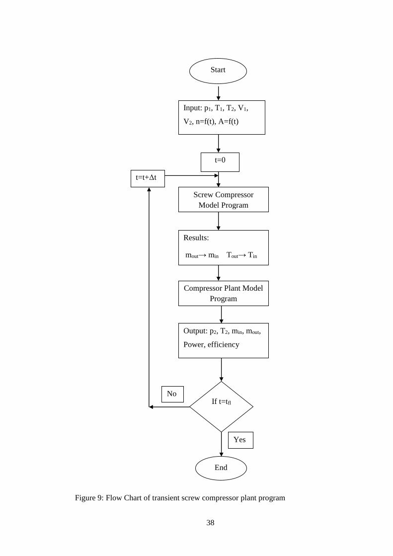
The algorithm used in the developed program is presented in Figure 9. When the

pressure p2 in the tank at each time step is known, the flow and temperature min and

Tin, at the compressor discharge, can be calculated. These derived values are then taken

as the input parameters for the next time step. When the tank pressure p2 is calculated,

mout is either known, or calculated, as for the flow through the exit throttle valve to

pressure p0, and T2 becomes Tout in the next time step. The calculation is repeated until

the final time is reached.

Mass inflow and outflow are calculated as pipe flow with restrictions which comprise

both line and local losses, thereby defining pressure drops within the plant

connections. Since the tanks are of far greater volume than the connections, which

results in far lower gas velocities within them, the losses in the tanks are far lower than

the pipe losses and can be neglected.

Two levels of programming were applied. Firstly the compressor and plant processes

were solved separately. The compressor process was calculated through the software

suite which simulates the screw compressor process. The results from the compressor

program were used as inputs to the plant program allowing the plant process to be

calculated. The results were presented in tabular and graphical form by the use of

Excel, with mutual interchange of their input and output data. This speeded the

calculation, allowing the bulk estimation of the unsteady behaviour of a screw

compressor plant under various scenarios.

38

Figure 9: Flow Chart of transient screw compressor plant program

Start

Input: p1, T1, T2, V1,

V2, n=f(t), A=f(t)

t=0

Screw Compressor

Model Program

Results:

mout→ min Tout→ Tin

Compressor Plant Model

Program

Output: p2, T2, min, mout,

Power, efficiency

t=t+Δt

End

If t=tfl

Yes

No

39

6. Startup Test Results and Data Analysis

The first tests were to investigate the startup characteristics of air oil-injected screw

compressor plant as a transient process in order to verify the utilisation of the simple

filling tank program as a first step in the development of a more advanced model in

the future.

6.1 Verification of Filling Tank Simulation

The simulation process of the tests was straightforward, because the discharge valve

was closed and the analytical model was very simple, while the full model is presented

in Chapter 5. As shown in Figure 10 and Figure 11, the simulated and measured results

agree closely.

Figure 10: Measured and predicted rates of pressure rise in the tank during compressor

startup when the starting pressure is 5 bar

This indicated that the model could be used to simulate the compressor startup and

shutdown. The next step was to use this program to simulate some interesting

situations during the startup as, for example, rapid change of shaft speed, and variation

of pressure or change in the tank volume. This gave an insight into what happens to

the system pressure immediately after the parameters are changed.

0

1

2

3

4

5

6

7

8

9

0 2 4 6 8 10 12

Pre

ssu

re,

ba

r

Time, s

Start from 5 bar at discharge

measured simulated

40

Figure 11: Measured and predicted rates of pressure rise in the tank during compressor

startup when the starting pressure is 7 bar

6.2. Data Analysis

As already stated, the aim of these tests was to determine the behaviour of the

compressor before oil injection started. It was expected that, during startup, the

temperature would rise quickly before the oil enters the working chamber. This might

result in damage to the rotor surfaces. Frequent start-stop operation may, therefore,

lead to wear and a rapid decrease in the compressor performance.

It can be seen from Figure 12 that when the compressor started from atmospheric

pressure, the temperature increases from 55 up to 100oC and after 8 seconds it

decreases to 90oC due to the development of oil injection. It needed some time for the

pressure to build-up in the oil reservoir and for oil to enter the compressor as a result

of the pressure difference.

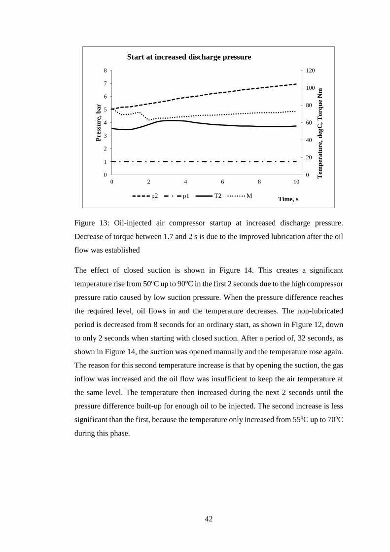
The situation is different when the compressor starts with its discharge pressure higher

than the inlet pressure, as shown in Figure 13. In this case, when the compressor stops,

oil flows into the compressor due to the pressure difference, but since the rotors are

not revolving, the compressor will fill with oil. So, when it starts to rotate, again, the

0

2

4

6

8

10

12

0 2 4 6 8 10 12

Pre

ssu

re,

ba

r

Time, s


measured simulated

41

oil within it will flow out through the compressor discharge port and the temperature

will immediately decrease. Soon afterwards, it stabilises. However, as shown in Figure

12 and Figure 13 when the compressor stops at atmospheric discharge pressure, the

discharge port is open and all the oil flows out of it. As a consequence, when the

compressor starts, it contains no oil and there is no pressure difference to promote its

flow. This period of dry contact between the rotors, can be reduced by closing both,

the compressor suction and discharge during the start. When the compressor starts, a

pressure difference develops immediately due to the pressure drop in the compressor

suction.

Figure 12: Oil-injected air compressor startup characteristics when discharging at

atmospheric pressure

0

20

40

60

80

100

120

0

1

2

3

4

5

6

7

8

0 2 4 6 8 10

Pre

ssu

re,

ba

r

Start from atmospheric pressure at discharge

p2 p1 T2 MTime, s

Tem

per

atu

re,

deg

C,

To

rqu

e, N

m

42

Figure 13: Oil-injected air compressor startup at increased discharge pressure.

Decrease of torque between 1.7 and 2 s is due to the improved lubrication after the oil

flow was established

The effect of closed suction is shown in Figure 14. This creates a significant

temperature rise from 50oC up to 90oC in the first 2 seconds due to the high compressor

pressure ratio caused by low suction pressure. When the pressure difference reaches

the required level, oil flows in and the temperature decreases. The non-lubricated

period is decreased from 8 seconds for an ordinary start, as shown in Figure 12, down

to only 2 seconds when starting with closed suction. After a period of, 32 seconds, as

shown in Figure 14, the suction was opened manually and the temperature rose again.

The reason for this second temperature increase is that by opening the suction, the gas

inflow was increased and the oil flow was insufficient to keep the air temperature at

the same level. The temperature then increased during the next 2 seconds until the

pressure difference built-up for enough oil to be injected. The second increase is less

significant than the first, because the temperature only increased from 55oC up to 70oC

during this phase.

0

20

40

60

80

100

120

0

1

2

3

4

5

6

7

8

0 2 4 6 8 10

Pre

ssu

re,

ba

r

Start at increased discharge pressure

p2 p1 T2 M

Tem

per

atu

re,

deg

C,

To

rqu

e N

m

Time, s

43

Figure 14: Oil-injected air compressor start with closed suction

There are other advantages to starting the compressor with closed suction because, as

the compressor starts in this manner, the suction pressure decreases below atmospheric

pressure and the air flow is almost zero. However, the discharge pressure will be equal

to the atmospheric pressure, as in the case when the discharge is open. As can be seen

in Figure 15, where the starting torque required is compared to the case shown in

Figure 12, and that in Figure 14, it follows that due to the small pressure difference

between inlet and discharge pressures, the peak torque is approximately one third

lower than during start with open suction, while the starting torque is approximately

four times less. As a consequence, this will result in a safer start, lower power

consumption and, less noise. This procedure is applied by many screw compressor

manufactures.

0

20

40

60

80

100

120

0

1

2

3

4

5

6

7

8

0 2 4 6 8 30 32 34 36 38 40

Pre

ssu

re,

ba

r

Start with closed suction

p2 p1 T2 M

Tem

per

atu

re,

deg

C,

To

rqu

e, N

m

Time, s

44

Figure 15: Comparison of startup with open and closed suction for oil-injected air

compressor, Upper graph shows Torque, Lower graph shows discharge pressure

0

5

10

15

20

25

30

35

40

45

50

0 0.5 1 1.5 2 2.5 3 3.5 4 4.5 5 5.5 6 6.5 7 7.5 8 8.5 9 9.5 10

To

rqu

e, N

m

Time, s

Torque

Open suction/Open discharge Closed suction/Open discharge

0.0

0.2

0.4

0.6

0.8

1.0

1.2

1.4

1.6

1.8

2.0

0 0.5 1 1.5 2 2.5 3 3.5 4 4.5 5 5.5 6 6.5 7 7.5 8 8.5 9 9.5 10

Dis

cha

rge

pre

ssu

re,

ba

r

Time, s

Discharge Pressure

Open suction/Open discharge Closed suction/Open discharge

45

It was found, from further startup tests with closed suction, that it took a longer time

to reach 3000rpm as the discharge pressure was increased, as shown in Figure 16 and

Figure 17. It is clear that the slowest start and the lowest acceleration were achieved

at 7 bar discharge, which was the highest pressure achieved. It was not possible to start

the compressor at discharge pressures above this value, due to limitation of the motor

current.


pressures, for clarity, the same starting point is assumed fo all cases

0

500

1000

1500

2000

2500

3000

3500

1 2 3 4 5

Sp

eed

, rp

m

Time, s7 bar 6 bar 5 bar

Speed

46

Figure 17: Startup times for oil-injected air compressor at different discharge pressures

Figure 18: Startup torque variation with discharge pressure for oil-injected air

compressor

As shown in Figure 18, the torque variation, during startup, follows a similar trend,

with the demand increasing as the discharge pressure is raised with the initial value,

0

500

1000

1500

2000

2500

3000

3500

0 0.5 1 1.5 2 2.5 3 3.5 4 4.5 5 5.5 6 6.5 7 7.5 8 8.5 9 9.5 10

Sp

eed

, rp

m

Time, s

Speed

7 bar at discharge 6 bar at discharge 5 bar at discharge

0

20

40

60

80

100

120

0 1 2 3 4 5 6 7 8 9 10

To

rqu

e, N

m

Time, s

Start with increased discharge pressure

7 bar at discharge 6 bar at discharge 5 bar at discharge

47

at rest, falling. However, as shown in, there is a reversal in the trend of the startup

discharge pressure, which rises, immediately at 5 bar, but which falls initially at 6 bar

and 7 bar, before starting to rise.

This follows because the internal discharge pressure of compressor is 4.7 bar but the

pressure in the pipe was measured straight after the discharge and is shown in Figure

19. Accordingly, as soon as compressor started running and the discharge port was

opened, there was a pressure drop when the pressure in the pipe was 6 and 7 bar.

However, when pressure in the pipe was 5 bar, it started to increase immediately.

Figure 19: Discharge pressure curves for oil-injected air compressor startups at

different pressures

6.3. Torque Classification and Moment of Inertia Quantification

The thermodynamic process, the pressure forces acting on the rotors and the shaft

torque were all estimated using DISCO, the proprietary software package for the

analysis of screw compressor performance, prepared in house, of which some details

are already given in Chapter 5. This was written to predict compressor behaviour

4

5

6

7

8

0 1 2 3 4 5 6 7 8 9 10

Pre

ssu

re,

ba

r

Time, s

Discharge pressure

discharge 7 bar discharge 6 bar discharge 5 bar

48

during steady state operation, but was used here, in a sequence of calculations, to

derive values at each discreet time, and thus, to simulate unsteady behaviour and to

quantify inertial effects during the compressor startup.

The simulation results obtained from the thermodynamic model are different to those

obtained from the test data, as shown in Figure 20 for the case of the compressor

starting at a discharge pressure of 7 bar.

Figure 20: Comparison between simulated and measured Speed and Torque changes

for oil-injected air compressor at a discharge pressure of 7 bar

The difference between the simulated torque, with mechanical losses taken into

account, as extrapolated, and the measured values, during the first 4 seconds can be

explained as due to rotor inertia in the period between 0.5s and 4s and the increased

friction torque in the period between 0s and 0.5s. The simulation did not function at

speeds below 1000 rpm.

Diagrams for the compressor starting at both atmospheric pressure and increased

pressure at discharge are presented in Figure 21 and 22.

-50.0

0.0

50.0

100.0

150.0

200.0

250.0

300.0

0

10

20

30

40

50

60

70

80

90

100

0 0.5 1 1.5 2 2.5 3 3.5 4 4.5 5 5.5 6 6.5 7 7.5 8 8.5 9 9.5 10

To

rqu

e, N

m

Time, s


Torque measured

Simulated Torque with mech losses

acceleration

Speed

Linear (Simulated Torque with mech losses)S

pee

d,

1/s

, A

ccel

era

tio

n, 1

/s2

49


atmospheric pressure


above atmospheric pressure

Pressure torque could be estimated by the DISCO software and friction torque can be

estimated from the assumed mechanical efficiency but inertia torque can only be

derived from the difference between the measured and predicted values.

0

500

1000

1500

2000

2500

3000

3500

30

35

40

45

50

0 1 2 3 4 5

To

rqu

e, N

m

Time, s

Start from atmospheric pressure

at discharge

Torque Speed

0

500

1000

1500

2000

2500

3000

3500

60

70

80

90

100

0 1 2 3 4 5

To

rqu

e, N

m

Times, s

Start from above atmospheric pressure at discharge

Torque Speed

50

A qualitative analysis of starting torque curves, based on Figure 21 and Figure 22 is

given below, where the torque curves were analysed assuming the following:

Total torque = Pressure torque plus Friction torque plus Inertial torque

Table 4: Torque effects during oil-injected air compressor startup

Start from Atmospheric

Pressure at Discharge

Start from Increased Pressure at

Discharge

Pressure

Torque

Pressure torque increases

constantly until maximum

discharge pressure is

achieved.

Pressure torque is high since compressor

starts rotating. Pressure forces, which

affect torque, might be even higher in the

first fraction of a second since

compressor is full of oil during high

pressure start.

Friction

Torque

Inertia of moving parts

affects total torque at the

very beginning.

Inertia of moving parts affects total

torque at the very beginning. Again, as

compressor is flooded with oil, friction

torque may also increase.

Inertia

Torque

Inertia forces act while

compressor accelerates and

inertia torque tends to zero

when 3000 rpm is achieved,

torque drops after 2 seconds

on diagram.

Since compressor overcomes friction,

torque drops after 1.5s on the diagram,

and machine starts accelerating, inertia

forces affect total torque. Inertia torque

tends to zero after compressor achieves

3000 rpm, torque drop between 3.5s and

4s.

51

7. Screw Compressor Plant Model Validation

Following the initial tests on the transient behaviour of screw compressor systems, the

development of a software simulation model and initial comparisons between

measured and predicted system performance, this chapter contains a fuller comparison

between them. As was described in Chapter 4, both oil-free and oil-injected air

compressor plants were modelled and measured. Plant parameters, such as compressor

speed and starting pressure and temperature were used as initial conditions for

simulation studies. When the working fluid was assumed to be an ideal gas, one full

set of 300-800s of real compressor operating time required 5-10 minutes of computer

calculation time, using a PC with an Intel Core2 Duo CPU 2.33GHz, with 4 GB of

RAM. When the working fluid was assumed to be a real gas the calculation time took

eight to ten times longer.

7.1. Oil-injected compressor

Figure 23: Comparison of estimated and measured pressure changes in oil-injected air

screw compressor plant. Differences < 5%

During the experiment the compressor speed was varied from 2000 up to 5000 rpm,

and back, in step changes of 1000 rpm, each within a time interval of 60 seconds,

which was sufficient time for the pressure to stabilise after the speed was changed.

0

1000

2000

3000

4000

5000

6000

0

2

4

6

8

10

12

0 200 400 600 800

Pre

ssu

re,

ba

r

Time, s

Pressure

Experiment Simulation Speed

Sp

eed

, rp

m

52

Variation of the main parameters with time is presented in following diagrams and

shows good agreement between experimental and simulated results.

Figure 24: Comparison of estimated and measured temperature changes in oil-injected

air screw compressor plant. Differences < 5%


injected air screw compressor plant. Differences < 5%

0

1000

2000

3000

4000

5000

6000

0

50

100

150

200

250

300

350

0 200 400 600 800

Tem

per

atu

re,

K

Time, s

Temperature


Sp

eed

, rp

m

0

1000

2000

3000

4000

5000

6000

0

0.02

0.04

0.06

0.08

0.1

0.12

0.14

0 200 400 600 800

Ma

ss f

low

, k

g/s

Time, s

Mass flow


Sp

eed

, rp

m

53

Figure 26: Comparison of estimated and measured input power changes in oil-injected


A comparison between the measured and simulated performance of an oil-injected

compressor plant is shown in Figure 23 to 26, when increasing and decreasing the

rotational speed between 2000 rpm and 5000 rpm. The difference between the

measured and predicted values of pressure, mass flow, power and temperature, are less

than 5% of the absolute values, in all cases. This indicates the basic suitability of the

predictive model for further development The greatest discrepancy was in the

estimated and measured temperature at a rotational speed of 2000 rpm, when the

difference was approximately 15oC. A possible reason for this is the low compressor

speed. This strongly affects leakage and could therefore have a substantial influence

on the temperature.

A further case is demonstrated in Figure 27 to 30, where the compressor speed was

increased directly from 3000 rpm to 5000 rpm and back. Even better agreement was

obtained for the same parameters in this case.

.

0

1000

2000

3000

4000

5000

6000

0

5

10

15

20

25

30

35

40

45

50

0 200 400 600 800

Po

wer

, k

W

Time, s

Power


Sp

eed

, rp

m

54

Figure 27: Comparison of estimated and measured pressure changes in oil-injected air


Figure 28: Comparison of estimated and measured temperature changes in oil-injected


0

1000

2000

3000

4000

5000

6000

0

2

4

6

8

10

12

0 50 100 150 200 250 300 350

Pre

ssu

re,

ba

r

Time, s

Pressure


Sp

eed

, rp

m

0

1000

2000

3000

4000

5000

6000

0

50

100

150

200

250

300

350

0 50 100 150 200 250 300 350

Tem

per

atu

re,

K

Time, s

Temperature


Sp

eed

, rp

m

55


injected air screw compressor plant. Differences < 5%

Figure 30: Comparison of estimated and measured input power changes in oil-injected


0

1000

2000

3000

4000

5000

6000

0

0.02

0.04

0.06

0.08

0.1

0.12

0.14

0 50 100 150 200 250 300 350

Ma

ss f

low

, k

g/s

Time, s

Mass flow


Sp

eed

, rp

m

0

1000

2000

3000

4000

5000

6000

0

5

10

15

20

25

30

35

40

45

50

0 50 100 150 200 250 300 350

Po

wer

, k

W

Time, s

Power


Sp

eed

, rp

m

56

7.2. Oil-Free Compressor

A comparison between the measured and predicted performance of an oil-free air

screw compressor plant is shown in Figure 31 to Figure 34. The compressor speed was

chosen as a variable parameter for transient analysis and it was varied from 3000 rpm

up to 9000 rpm and then back in steps of 2000 rpm and time intervals of approximately

30 seconds. This was sufficient time for the pressure to stabilise after the speed was

changed. As can be seen, the pressure in the oil-free compressor changed almost

immediately after the speed was changed, while the pressure in the oil-injected

changed gradually. The lag in Figure 23, may be due to the oil thickness which creates

some inertia effect.

All the parameters shown in Figure 31 to Figure 34 are within acceptable 5%

difference of their absolute values, although the temperature discrepancy shown in

Figure 32, is present again, as in the case of the oil-injected machine.

It can be seen from Figure 32, that the calculated values of temperature are 'symmetric',

i.e. the acceleration and deceleration values are similar after some time spent at a given

speed. However, the experimental air temperature values are higher for deceleration

than for acceleration, because it is necessary to heat the tank and pipes up during

acceleration. This requires time, therefore, the air is cooled during that process and it

will show a lower temperature than it would be if there were` no heat transfer between

the air and the pipes. During deceleration however, the higher temperature of the

recently heated pipes causes the air to be heated up during that process and thus it

shows higher temperature values if compared with acceleration. This confirms, once

again, that the model is working properly and can be used by other investigators.

57

Figure 31: Comparison of estimated and measured pressure changes in oil free air


Figure 32: Comparison of estimated and measured temperature changes in oil free air


0

1000

2000

3000

4000

5000

6000

7000

8000

9000

0

0.5

1

1.5

2

2.5

0 50 100 150 200 250 300

Pre

ssu

re,

ba

r

Time, s

Pressure


Sp

eed

, rp

m

0

1000

2000

3000

4000

5000

6000

7000

8000

9000

0

50

100

150

200

250

300

350

400

450

0 50 100 150 200 250 300

Tem

per

atu

re,

K

Time, s

Temperature


Sp

eed

, rp

m

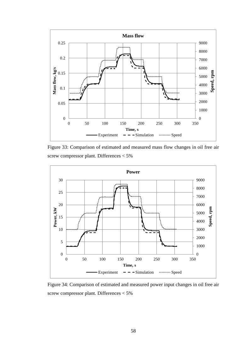
58

Figure 33: Comparison of estimated and measured mass flow changes in oil free air


Figure 34: Comparison of estimated and measured power input changes in oil free air


0

1000

2000

3000

4000

5000

6000

7000

8000

9000

0

0.05

0.1

0.15

0.2

0.25

0 50 100 150 200 250 300 350

Ma

ss f

low

, k

g/s

Time, s

Mass flow


Sp

eed

, rp

m

0

1000

2000

3000

4000

5000

6000

7000

8000

9000

0

5

10

15

20

25

30

0 50 100 150 200 250 300 350

Po

wer

, k

W

Time, s

Power


Sp

eed

, rp

m

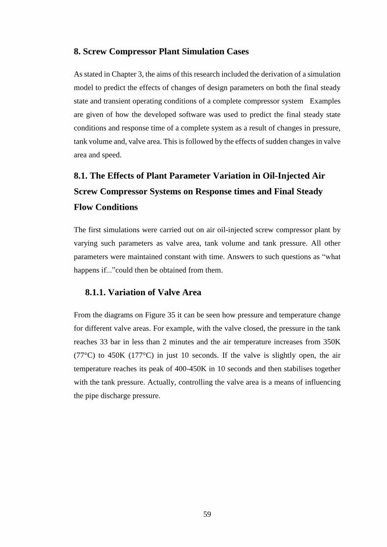
59

8. Screw Compressor Plant Simulation Cases

As stated in Chapter 3, the aims of this research included the derivation of a simulation

model to predict the effects of changes of design parameters on both the final steady

state and transient operating conditions of a complete compressor system Examples

are given of how the developed software was used to predict the final steady state

conditions and response time of a complete system as a result of changes in pressure,

tank volume and, valve area. This is followed by the effects of sudden changes in valve

area and speed.

8.1. The Effects of Plant Parameter Variation in Oil-Injected Air

Screw Compressor Systems on Response times and Final Steady

Flow Conditions

The first simulations were carried out on air oil-injected screw compressor plant by

varying such parameters as valve area, tank volume and tank pressure. All other

parameters were maintained constant with time. Answers to such questions as “what

happens if...”could then be obtained from them.

8.1.1. Variation of Valve Area

From the diagrams on Figure 35 it can be seen how pressure and temperature change

for different valve areas. For example, with the valve closed, the pressure in the tank

reaches 33 bar in less than 2 minutes and the air temperature increases from 350K

(77°C) to 450K (177°C) in just 10 seconds. If the valve is slightly open, the air

temperature reaches its peak of 400-450K in 10 seconds and then stabilises together

with the tank pressure. Actually, controlling the valve area is a means of influencing

the pipe discharge pressure.

60

Figure 35: The effect of varying the valve area in an oil-injected air screw compressor

plant. The upper graph shows the Tank Pressure, and the lower graph shows the

Temperature

8.1.2. Varying the Tank Volume

It is evident from the diagram in Figure 36 that, for a given throttle valve area, the

final discharge pressure will be independent of the tank volume and changes in the

latter will only affect the time required to reach steady stage conditions. Thus with a

0

5

10

15

20

25

30

35

40

0 20 40 60 80 100

Pre

ssu

re,

ba

r

Time, s

70mm2 50mm2 30mm2 closed valve

300

350

400

450

500

0 20 40 60 80 100

Tem

per

atu

re,

K

Time, s

70mm2 50mm2 30mm2 closed valve

61

30 litre tanks steady conditions are attained in 2 seconds, but for a 600 litre tank the

time taken is about 2 minutes. A similar situation happens with the temperature: when

its peak value of 420-450K is attained more rapidly with a smaller volume, before

returnings to the initial value of 350K.

Figure 36: The effect of varying the tank volume in an oil-injected air screw


shows the Temperature

0.0

0.5

1.0

1.5

2.0

2.5

3.0

3.5

4.0

4.5

0 20 40 60 80 100

Pre

ssu

re,

ba

r

Time, s

0.03 m3 0.1 m3 0.3 m3 0.6 m3

300

350

400

450

500

0 20 40 60 80 100

Tem

per

atu

re,

K

Time, s

0.03 m3 0.1 m3 0.3 m3 0.6 m3

62

8.1.3. Varying the Tank Pressure

As shown in Figure 37, regardless of its initial value, the final pressure achieved in the

tank is determined by the valve area. Thus, as already shown in Figure 36, the final

discharge conditions in the pipe are a pressure of 4.2 bar and a temperature of 350K,

whether the initial pressure is higher or lower than this value.

Figure 37: The effect of varying the initial tank pressure in an oil-injected air screw


shows the Temperature

0

1

2

3

4

5

6

7

8

0 20 40 60 80 100

Pre

ssu

re,

ba

r

Time, s

1 bar 3 bar 5 bar 7 bar

300

325

350

375

400

425

450

0 20 40 60 80 100

Tem

per

atu

re,

K

Time, s

1 bar 3 bar 5 bar 7 bar

63

As can be seen from all the given diagrams, the results, obtained from the compressor

plant model, agree with the laws of Physics and provide a solid basis for extending its

use for unsteady plant simulation in more complex applications.

8.2. Closed loop Screw Compressor Plant Simulations

The single tank model in an open plant system can be adapted to simulate a compressor

system containing two tanks operating in a closed loop, with gases, refrigerants or air

as the contained working fluid.

Figure 38: Two tank closed loop screw compressor plant system

As shown in Figure 38, air, or any other gas, leaves Tank 1 to enter the screw

compressor, from which it is discharged into Tank 2, to return to Tank1, via a throttle

valve. It is assumed, for this and all further simulations, that the volume of Tank 1 is

much larger than that of Tank 2.

For a given compressor speed, the steady state pressures in the two tanks, attained after

startup, are determined by the valve area. Thus, reducing the valve area, decreases the

flow into Tank 1 and then into Tank2, thereby resulting in a lower preessure in Tank

1. Conversely, opening the valve will increase the pressure in Tank 1 after the

compressor starts, but in both cases, for a fixed valve area, the system will stabilise to

maintain constant pressure in both tanks.

64

8.2.1. Varying the Compressor Shaft Speed in a Closed Loop

System

The effect of varying the compressor rotational speed, for a fixed starting pressure is

shown in Figure 39. As can be seen, because Tank 1 is much larger than Tank 2, the

pressure remains constant for shaft speed 4500 rpm and it converges to a higher or

lower value if the speed is increased or decreased.

Figure 39: Pressure variation in the discharge Tank, as a result of speed changes in a

closed loop air screw compressor plant

At constant speed, the mass flow into the discharge tank (Tank 2) remains constant,

but as the speed is increased, it may be seen that for the steady case at n=4500 rpm, as

shown in Figure 39 and Figure 40, as the speed is increased, the mass flow into Tank

1 rises. Conversely, when the shaft speed is decreased, the mass flow entering Tank1

decreases until it equals the mass flow into the Tank2, resulting in a rise in pressure in

Tank 1 and a fall in pressure in Tank 2.

0

2

4

6

8

10

12

14

0 5 10 15 20

Pre

ssu

re,

Pa

Time, s

n=3000rpm n=6000rpm n=4500rpm

65

Figure 40: Mass flow going to both tanks at different shaft speeds

8.2.2. Variation of Shaft Speed during Compressor Operation in

a Closed Loop System

The next simulation case was to determine the effects of a sudden change in the

compressor speed while the system was in operation. The result is shown in Figure 41.

As soon as the speed increased from 3000 rpm to 6000rpm, the pressure in Tank2

started to increase slowly but the pressure in Tank 1 remained constant because the

volume of Tank 1 is much larger than that of Tank 2. However, as shown in Figure

42, the mass flow into the Tank 2 is doubled immediately because the inflow is

proportional to the shaft speed, but it took about 10 seconds for flow into Tank1 to

reach to the same value.

0.00

0.02

0.04

0.06

0.08

0.10

0.12

0.14

0.16

0.18

0 5 10 15 20

Ma

ss f

low

, k

g/s

Time, s

3000rpm, tank1 6000rpm, tank1 4500rpm, tank1

0.00

0.02

0.04

0.06

0.08

0.10

0.12

0.14

0.16

0.18

0 5 10 15 20

Ma

ss f

low

, k

g/s

Time, s

3000rpm, tank2 6000rpm, tank2 4500rpm, tank2

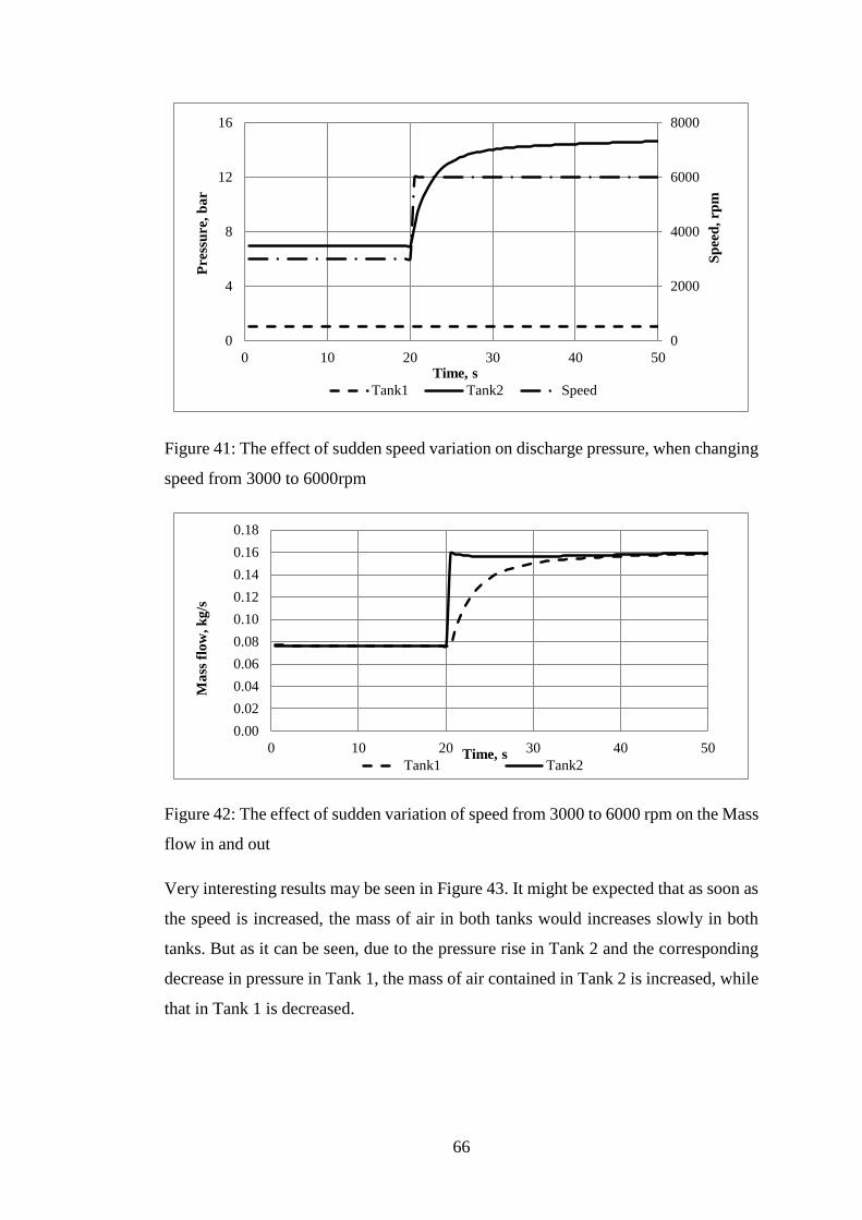
66

Figure 41: The effect of sudden speed variation on discharge pressure, when changing

speed from 3000 to 6000rpm

Figure 42: The effect of sudden variation of speed from 3000 to 6000 rpm on the Mass

flow in and out

Very interesting results may be seen in Figure 43. It might be expected that as soon as

the speed is increased, the mass of air in both tanks would increases slowly in both

tanks. But as it can be seen, due to the pressure rise in Tank 2 and the corresponding

decrease in pressure in Tank 1, the mass of air contained in Tank 2 is increased, while

that in Tank 1 is decreased.

0

2000

4000

6000

8000

0

4

8

12

16

0 10 20 30 40 50

Sp

eed

, rp

m

Pre

ssu

re,

ba

r

Time, s

Tank1 Tank2 Speed

0.00

0.02

0.04

0.06

0.08

0.10

0.12

0.14

0.16

0.18

0 10 20 30 40 50

Ma

ss f

low

, k

g/s

Time, sTank1 Tank2

67

Figure 43: Change of mass of air in both tanks, as a result of changing speed from

3000 to 6000rpm

Figure 44: Pressure changes in both tanks, resulting from speed changes from 3000 to

6000rpm and back to 3000

Another example is presented in Figure 44 where the compressor speed is suddenly

increased from 3000 rpm to 6000 rpm and subsequently, suddenly reduced back to

3000 rpm. The pressure in Tank1 will not change substantially because its volume is

much larger than of Tank 2. The pressure in Tank 2 increases gradually as soon as the

speed is increased and returns back to the same pressure of 7 bar when the speed

returns to 3000rpm.

59.0

59.5

60.0

60.5

61.0

0.00

0.10

0.20

0.30

0.40

0.50

0.60

0.70

0 10 20 30 40 50

Ma

ss o

f a

ir,T

an

k1

, k

g

Ma

ss o

f a

ir,

Ta

nk

2 k

g

Time, s

Tank2 Tank1

0

2000

4000

6000

8000

0

4

8

12

16

0 20 40 60 80

Sp

eed

, rp

m

Pre

ssu

re, b

ar

Time, s

Tank1 Tank2 Speed

68

8.3. Simulation of Multiple Tank Screw Compressor Plant

Figure 45: Compressor plant layout for multiple tank configuration

As has been stated before, the model may be used to simulate all types of configuration

and consequent unsteady conditions which may be found in real plant. An example

of a multiple tank configuration is shown in Figure 45, where there are three tanks.

This was also investigated assuming the same initial values of starting pressure

p1=1bar, discharge pressure p2=5bar, and starting temperature T=303K. The

possibilities considered are presented in Table 5 and examples given for each case.

Table 5: Scenarios plan

Scenario 1 Scenario 2 Scenario 3

V2=V3 V2=V3 V2≠V3

Δt≠const Av2≠Av3 Av2≠Av3

8.3.1. Scenario 1: Time Variation

As shown in Figure 45, Tank1 is much bigger than others, while the volumes of Tank2

and Tank3 are equal, as well as the valve areas Av2 and Av3. For Case1, the

compressor speed varies from 3000 rpm to 6000 rpm and back for successive periods

of 25s in Case1, 50s in Case2 and 100s in Case3.

69

Figure 46: Pressure variation in Tank 2 and Tank 3 for different cycle time Intervals

0

1000

2000

3000

4000

5000

6000

7000

0.00E+00

2.00E+05

4.00E+05

6.00E+05

8.00E+05

1.00E+06

1.20E+06

0 100 200 300 400

Pre

ssu

re,

Pa

Time, s

Case1: Δt=25sec

Pressure, Tank2 Pressure, Tank 3 Speed

Sp

eed

, rp

m

0

1000

2000

3000

4000

5000

6000

7000

0.00E+00

2.00E+05

4.00E+05

6.00E+05

8.00E+05

1.00E+06

1.20E+06

0 100 200 300 400

Pre

ssu

re,

Pa

Time, s

Case 2: Δt= 50 sec

Pressure, Tank 2 Pressure, Tank 3 SpeedS

pee

d,

rpm

0

1000

2000

3000

4000

5000

6000

7000

0.00E+00

2.00E+05

4.00E+05

6.00E+05

8.00E+05

1.00E+06

1.20E+06

0 100 200 300 400 500 600

Pre

ssu

re,

Pa

Time s

Case 3: Δt= 100 sec

Pressure, tank 2 Pressure, Tank 3 Speed

Sp

eed

, rp

m

70

Figure 47: Temperature variation in Tank2 and Tank3 for different cycle time intervals

0

1000

2000

3000

4000

5000

6000

7000

250

270

290

310

330

350

370

0 100 200 300 400

Tem

per

atu

re,

K

Time, s

Case 2: Δt= 50 sec

Temperature, Tank2 Temperature, Tank 3 SpeedS

pee

d,

rpm

0

1000

2000

3000

4000

5000

6000

7000

250

270

290

310

330

350

370

0 100 200 300 400 500 600

Tem

per

atu

re,

K

Time, s

Case 3: Δt= 100 sec

Temperature, Tank 2 Temperature, Tank 3 Speed

Sp

eed

, rp

m

0

1000

2000

3000

4000

5000

6000

7000

250

270

290

310

330

350

370

0 100 200 300 400

Tem

per

atu

e, K

Time, s

Case1: Δt=25sec


Sp

eed

, rp

m

71

Tank2 and Tank3 are downstream of the compressor and it can be seen from Figure

46 and Figure 47 how the pressure and temperature vary for each of the three cycle

times. If Tank2 is considered, it can be seen that pressure would rise further in Case1

if Δt were longer, but it attains a maximum of 10 bar for Case2 and Case3. Although

the pressure rose from 5 to 10 bar in both cases 2 and 3, the larger time interval

between cycles, in Case3, enabled steady conditions to be maintained for a longer

period . The temperature changes shown in Figure 47 confirm the same trends, namely,

the maximum and the minimum values are the same for all three cases but the larger

cycle times enable steady conditions to be attained for longer periods with sharper

peaks. This is another illustration of the advantages of a dynamic model rather than

estimating the extreme conditions, using a steady state model.

8.3.2. Scenario 2: Valve Area Variation

Scenario 2 includes 5 cases: valve areas are equal in the beginning but then valves

Av2 or Av3 can be varied, as given in Table 6.

Cases 1-2-3 and Cases 1-4-5 are considered separately.

Table 6: Valve area variation cases

Case № Av2 Av3

Case 1 1.2 1.2

Case 2 1.2 0.8

Case 3 1.2 1.6

Case 4 0.8 1.2

Case 5 1.6 1.2

The pressure and power for these cases are given in Figure 48. As soon as valve Av3

is closed in Case 2, the power input increases from 62 to 70 kW when the compressor

speed n=6000 rpm, the pressure in Tank 2 rises from 8 to 10.3bar and in Tank 3 – from

5.3 to 7.8 bar. The power does not change so significantly when the speed is 3000 rpm.

When valve Av3 is closed, air starts to accumulate in both tanks and causes both the

pressure and the input power to rise. When valve Av3 is opened, in Case 3, it can be

seen that the pressure and power decrease.

72

Figure 48: Pressure in Tank2 and Tank3 and input power for cases 1-5

0.00E+00

2.00E+05

4.00E+05

6.00E+05

8.00E+05

1.00E+06

1.20E+06

0 100 200 300 400 500 600

Pre

ssu

re,

Pa

Time, s

Pressure, Tank 2, cases 1-5

Case 1

Case 2

Case 3

Case 4

Case 5

0.00E+00

1.00E+05

2.00E+05

3.00E+05

4.00E+05

5.00E+05

6.00E+05

7.00E+05

8.00E+05

9.00E+05

0 100 200 300 400 500 600

Pre

ssu

re,

Pa

Time, s

Pressure, Tank 3, cases 1-5

Case 1

Case 2

Case 3

Case 4

Case 5

0

10,000

20,000

30,000

40,000

50,000

60,000

70,000

80,000

0 100 200 300 400 500 600

Po

wer

, W

t

Time, s

Power for cases 1-5

Case 1

Case 2

Case 3

Case 4

Case 5

73

When valve Av2 is closed, air starts to accumulate in Tank 2 and this causes the

pressure in it to rise from 8 to 10.3 bar at compressor speed 6000rpm and from 4 to 5

bar at 3000rpm, power rises at high speed only, from 62kW to 70kW, although

pressure in the Tank3 is similar. Diagrams show that pressure and power drop down

when valve Av2 open.

8.3.3. Scenario 3: Valve Area and Tank Volume Variation

Figure 49: Compressor plant layout for multiple tank configuration

The multiple tank system presented in Figure 49 is similar to that in Figure 45, but

the volume of Tank2 is twice that of Tank3, i.e.V2=2V3. Three different cases were

considered, when the valve area between the tanks varies; namely: Av2=Av3 in Case1,

Av2=2Av3 in Case2 and Av3=1.5Av2 in Case3. The initial temperatures and pressures

are the same as in the previous cases. Again, it can be clearly seen that the pressure

rise varies for different valve areas, namely: the more the valve is open, the faster the

pressure rise, as shown in Figure 50. So, it is important to understand plant dynamics

properly when the system performance is analysed. For Case2, when the second valve

has a small opening area, the pressure difference between the tanks is the least, at 1-2

bar, and the final pressure is the highest at 10-12 bar, because air accumulates in the

tanks due to the small area of Av3. Temperature dynamic is shown in Figure 51.

74

Figure 50: Rates of pressure change in Tank2 and Tank3 for varying valve areas and

tank capacities

0

1000

2000

3000

4000

5000

6000

7000

0.00E+00

1.00E+05

2.00E+05

3.00E+05

4.00E+05

5.00E+05

6.00E+05

7.00E+05

8.00E+05

9.00E+05

0 100 200 300 400 500 600

Pre

ssu

re,

Pa

Time, s

Case1: V2=2V3 and Av2=Av3

Pressure, Tank 2 Pressure, Tank 3 Speed

Sp

eed

, rp

m

0

1000

2000

3000

4000

5000

6000

7000

0.00E+00

2.00E+05

4.00E+05

6.00E+05

8.00E+05

1.00E+06

1.20E+06

1.40E+06

0 100 200 300 400 500 600

Pre

ssu

re,

Pa

Time s

Case2: V2=2V3 and Av2=2Av3


Sp

eed

, rp

m

0

1000

2000

3000

4000

5000

6000

7000

0.00E+00

1.00E+05

2.00E+05

3.00E+05

4.00E+05

5.00E+05

6.00E+05

7.00E+05

8.00E+05

0 100 200 300 400 500 600

Pre

ssu

re,

Pa

Time, s

Case3: V2=2V3 and 1.5Av2=Av3


Sp

eed

, rp

m

75

Figure 51: Rates of temperature change in Tank2 and Tank3 for varying valve areas

and tank capacities

0

1000

2000

3000

4000

5000

6000

7000

250

270

290

310

330

350

370

0 100 200 300 400 500 600

Tem

per

atu

re,

K

Time, s

Case1: V2=V3 and Av2=Av3


Sp

eed

, rp

m

0

1000

2000

3000

4000

5000

6000

7000

250

270

290

310

330

350

370

0 100 200 300 400 500 600

Tem

per

atu

re,

K

Time, s

Case2: V2=2V3 and Av2=2Av3


Sp

eed

, rp

m

0

1000

2000

3000

4000

5000

6000

7000

250

270

290

310

330

350

370

390

0 100 200 300 400 500 600

Tem

per

atu

re,

K

Time, s

Case3: V2=2V3 and 1.5Av2=Av3


Sp

eed

, rp

m

76

8.3.4. Scenario 4: Four Tank Compressor Plant

Figure 52: Four tank compressor plant configuration

A Further analysis was carried out for a four tank system, as shown in Figure 52 and

a comparison of the response rates with different numbers of tanks is given in Figure

53 and 54. As can be seen, the discharge pressure from the compressor increases with

the number of tanks in the system.

Figure 53: Pressure in the tank after compressor for 2-, 3- and 4-tank systems

0

1000

2000

3000

4000

5000

6000

0

2

4

6

8

10

12

14

100 150 200 250 300 350 400

Pre

ssu

re,

ba

r

Time, s

System of 2 Tanks System of 3 Tanks

System of 4 Tanks Shaft Speed

Sh

aft

S

pee

d,

rpm

77

Figure 54: Variation of pressure, above, and temperature, below, in three tank

compressor plant model depending on speed changes

Pressure and temperature changes in a three tank compressor plant, resulting from

speed changes, are shown in Figure 54. Although the speed was decreased before the

pressure stabilised, it can be seen that cycles are repetitive.

0

1000

2000

3000

4000

5000

6000

0

2

4

6

8

10

12

100 150 200 250 300 350 400

Pre

ssu

re,

ba

r

Time, s

Pressure in First Tank Pressure in Second Tank Shaft Speed

Sh

aft

S

pee

d,

rpm

0

1000

2000

3000

4000

5000

6000

300

325

350

375

400

425

450

100 150 200 250 300 350 400

Tem

per

atu

re,

K

Time, s

Temperature in First Tank Temperature in Second Tank Shaft Speed

Sh

aft

S

pee

d,

rpm

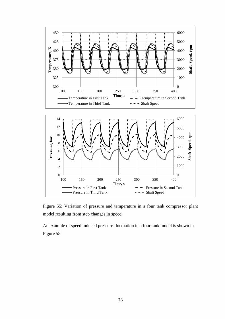
78

Figure 55: Variation of pressure and temperature in a four tank compressor plant

model resulting from step changes in speed.

An example of speed induced pressure fluctuation in a four tank model is shown in

Figure 55.

0

1000

2000

3000

4000

5000

6000

300

325

350

375

400

425

450

100 150 200 250 300 350 400

Tem

per

atu

re,

K

Time, sTemperature in First Tank Temperature in Second Tank

Temperature in Third Tank Shaft Speed

Sh

aft

S

pee

d,

rpm

0

1000

2000

3000

4000

5000

6000

0

2

4

6

8

10

12

14

100 150 200 250 300 350 400

Pre

ssu

re,

ba

r

Time, sPressure in First Tank Pressure in Second Tank

Pressure in Third Tank Shaft SpeedS

ha

ft S

pee

d,

rpm

79

8.3.5. Scenario 5: Simulation of a Plant where the Tanks are

widely separated

Figure 56: Screw compressor plant with widely spaced tanks

Scenario 5 does not present any comparison, but give an example of real factory case

where dynamic program can be used to get any parameter value at any time. The

developed program is useful for complex facilities with air distribution systems. An

example of such plant can be illustrated as follows. Compressor and Tank2 are located

in building 1. There is need for pneumatic instruments in another building 2 where

Tank3 is located at distance L from building 1, as shown in Figure 56. The model

enables the dynamic response to parameter changes in both tanks to be investigated.

If pressure in Tank3 is at its required level and the compressor performance is defined,

the effects of possible variation in the pipe length L and its diameter dh can be

calculated. For example, if the compressor provides 5 bar at discharge, while the

required pressure, for instrumentation, is 4 bar and the distance between building 1

and building 2 is 15m. Using initial calculation results, a pipe diameter dh=25mm is

defined. This pipe can be replaced with a valve, across which the pressure drop is

equal to pressure drop in the pipe 1” and 15m length. Varying parameters of pressures,

tank volume, pipe and diameter length, compressor speed, it can be concluded how

80

these changes affect all parts of the system. Mass flow and pressure responses to speed

changes are shown in Figure 57.

Figure 57: Rates of pressure and mass flow change in a widely spaced tank system

Sample Calculation of the effects of pipe diameter change.

p2=5 bar, p3=4bar → Δp=1bar

then air velocity in a pipe is calculated:

𝑤 =𝑄

𝐴

where Q is volume flow, m3/s, A – area of the pipe, m2

Chosen pipe diameter is 25mm, volumetric flow is taken from results file of the

program

𝑤 =4.035 4

60𝜋0.0252

𝑤 = 137𝑚/𝑠

0.00E+00

2.00E-02

4.00E-02

6.00E-02

8.00E-02

1.00E-01

1.20E-01

1.40E-01

1.60E-01

1.80E-01

0.00E+00

2.00E+05

4.00E+05

6.00E+05

8.00E+05

1.00E+06

1.20E+06

0 100 200 300 400 500 600

Pre

ssu

re,

[Pa

] a

nd

Po

wer

[W

]

Time, s

Pressure, Tank 2 Pressure, Tank 3 Power

Mass flow, Tank 2 Mass flow, Tank 3

Ma

ss f

low

, [k

g/s

]

81

Then Reynolds number is calculated:

𝑅𝑒 =𝑤𝑑

𝑣

where kinematic viscosity is taken from the table for dry air and temperature 325K,

𝑣 = 1.807 × 10−5m2/s

𝑅𝑒 = 1.9 105

Figure 58: Moody diagram

Then, using the Moody diagram, given in Figure 58, the friction factor f is found, Re

and relative pipe roughness 0.001 were taken into account. Friction factor f=0.0215,

so, Darcy friction factor fd=4∙0.0215=0.086.

Also, as density had to be calculated, pressure and temperature are extracted from

result file the program.

𝜌 =𝑝

𝑅𝑇

𝜌 =5.03 105

287 320= 5.476 𝑘𝑔/𝑚3

82

Using the Darcy-Weisbach equation, the length of the pipe is found by use of given

pressure difference, pipe diameter etc.

∆𝑝 =8𝑓𝑑𝐿𝑄2

𝜋2𝜌𝑑5

Finally, for the diameter 25mm, length of the pipe is found as 15 m.

If the same procedure is repeated for 50mm pipe, length of the pipe is equal to 420m.

Similar calculations and simulations can be done for the system with unlimited

quantity of tanks similar to combination presented on Figure 59.

Figure 59: Alternative screw compressor plant scheme

83

8.4. Simulation of Steady and Intermittent Modes in order to

Estimate Plant Performance

A preliminary investigation was also carried out to determine how power consumption

differs between steady and intermittent operation as a result of varying the valve area.

Figure 60: Pressure variation in the tank resulting from sudden valve area changes

The results of the analysis of a case where the steady state discharge pressure is 7 bar

and the valve area is 50mm2 are shown in Figure 60 when the valve area varies

between 40 mm2 and 60 mm2. The power consumption for both cases was calculated

and the difference was found to be about 1%.

0

1

2

3

4

5

6

7

8

9

0 400 800 1200 1600 2000 2400 2800 3200 3600

Pre

ssu

re,

ba

r

Time, sSteady Unsteady

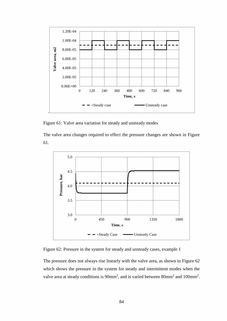
84

.

Figure 61: Valve area variation for steady and unsteady modes

The valve area changes required to effect the pressure changes are shown in Figure

61.

Figure 62: Pressure in the system for steady and unsteady cases, example 1

The pressure does not always rise linearly with the valve area, as shown in Figure 62

which shows the pressure in the system for steady and intermittent modes when the

valve area at steady conditions is 90mm2, and is varied between 80mm2 and 100mm2.

0.00E+00

2.00E-05

4.00E-05

6.00E-05

8.00E-05

1.00E-04

1.20E-04

0 120 240 360 480 600 720 840 960

Va

lve

are

a, m

2

Time, s

Steady case Unsteady case

3.0

3.5

4.0

4.5

5.0

0 450 900 1350 1800

Pre

ssu

re,

ba

r

Time, s

Steady Case Unsteady Case

85

Table 7: System parameter comparison, example 1

Steady Intermittent delta, %

Power kW 15.949 16.065 0.72

Sp. Power, kW/m3/min 4.081 4.112 0.76

As can be seen from Figure 62 and Table 7 the average power and specific power for

the steady and intermittent cases differ by approximately 1%. But if larger area

changes are made as shown in Figure 63 and Table 8, the pressure changes are of the

order of 12%, and power and specific power consumption change by 8-9%. And as

can be seen again, the pressure change with area is not linear.

Figure 63: Pressure variation in the system for steady and unsteady cases, example 2

Table 8: System parameters comparison, example 2

Steady Intermittent delta, %

Power kW 17.044 18.540 8.06

Sp. Power, kW/m3/min 4.378 4.791 8.62

0

1

2

3

4

5

6

7

8

0 450 900 1350 1800

Pre

ssu

re,

ba

r

Time, s

Steady Case Unsteady Case

86

8.5. Pressure Range Limit Simulation

Another scenario considered was how the pressure varies during intermittent

shutdown. The plant model was modified to include maximum and minimum speeds

as well as maximum and minimum pressures as input limiting conditions. The

program then simulated the process of the pressure rising at maximum speed until it

achieved its maximum value. The shaft speed then became equal to its minimum

speed, which was zero in our case since this corresponds to shut off. The pressure

then decreased until it attained its minimum value. The shaft speed then increased to

its maximum value and the entire process was repeated. The results of this study are

shown in Figure 63 and Table 9.

Figure 64: Pressure for simulated switch off and switch on

Table 9: Initial parameters of the system

V

[m3]

Speed

max

[rpm]

Speed

min

[rpm]

P max

[bar]

P min

[bar]

Av

[mm2]

Cycle

length,

[s]

Figure

0.325 6000 0 10.5 7.5 48.5 650 65

0.325 6000 0 8 6 58.5 25 66

87

Thus, the model enables all kind of scenarios for system shut down to be analysed and

enables the time it takes for the pressure to drop to pmin and then back to pmax and the

results are shown in Figure 65. This will vary depending on the tank volume or the

valve area for different initial values of smax/smin and pmax/pmin. and would be of value

for control engineers.

Figure 65: Pressure curve for simulated switch repetitive on/off operation

88

9. Conclusions

The intermittent character of everyday operation of industrial plant, using

compressors, requires special attention to be paid to ensure their reliable and efficient

operation. Systems operating with reciprocating and centrifugal machines have

previously been investigated and computer programs that simulate their operation

under these conditions already exist. But, due to the complex geometry of screw

compressors, no such programs were found to be available, in the public domain, to

analyse the performance of systems operating with these machines.

Accordingly, the aim of this research was to develop and verify a mathematical model

to analyse screw compressor driven plant during both continuous and intermittent

operation. This has been achieved by:

Development of a model, based on the differential equations of conservation

of mass and energy, which is suitable for air, process gas and refrigeration

plant by the inclusion of equations for the prediction of real gas properties;

The testing of this model by comparison of predicted performance with test

data. The difference between them is within 5% for all analysed parameters

and less than 2% for the majority of the cases considered;

The use of this model to predict a variety of operating scenarios. These include

any number of gas storage tanks of various sizes, located at different positions,

pressure reduction valves and condensers and evaporators;

The model can predict compressor plant performance such as power, specific

power and efficiency during intermittent operation. This enables the plant

performance to be estimated at any instant;

Startup and shutdown simulation can be performed within defined pressure

and speed intervals. This may be useful for control engineers.

89

10. Recommendations for Future Work

The model can be extended to expand possible options for modelling of screw

compressor plant operating under intermittent conditions. This includes, refrigeration

applications, which have been only mentioned in Chapter 8, and multiple tanks in

parallel, as shown in Figure 66. Also, experimental work can be further extended to

verify refrigeration plant predictions.

Figure 66: Multiple tank configuration for further modelling

.

90

Bibliography

Amosov, P. E., 1977. Vintovie kompressornye mashiny (Screw Compressors

Machines). Leningrad: Mashinostroenie.

Andreev, P. A., 1961. Vintovye kompressornye mashiny (Screw Compressor

Machines). Leningrad: SUDROM.

Anon., 2012. Honywell Process Solutions. [Online]

Available at: https://www.honeywellprocess.com/library/marketing/notes/service-

note-on-dynamic-engineering-studies.pdf

[Accessed March 2014].

Bendapudi, S. & Braun, J. E., 2002. A review of literature on dynamic models of

vapour compression equipment, s.l.: ASHRAE.

Bezzo, F. et al., 2004. Using Process Simulators for Steady-state and Dynamic Plant

Analysis. Chemical Engineering Research and Design, 82(A4), pp. 499-512.

Bloch, H. P., 2006. Compressors and modern process applications. Hoboken, New

Jersey: John Wiley&Sons.

Brownrigg, N., 2014. Protecting compressors with dynamic simulation, s.l.:

AspenTech.

Brown, R. N., 1997. Compressors: selection and sizing. Houston: Butterworth-

Teinemann.

Cetin Kocak, M., 1980. Dynamic Simulation of Chemical Plant. Birmingham:

University of Aston, Thesis.

Chukanova, E., Stosic, N. & Kovacevic, A., 2013. Experimental Investigation and

Numerical Modelling of Dynamic Behaviour of Screw Compressor Plant. Universal

Journal of Engineering Science, Volume 1, pp. 68-79.

Chukanova, E., Stosic, N. & Kovacevic, A., 2013. Numerical Analysis of Unsteady

Behaviour of a Screw Compressor System. London, s.n.

91

Chukanova, E., Stosic, N. & Kovacevic, A., 2014. Modelling and Experimental

Investigation of Unsteady Behaviour of a Screw Compressor Plant. London,

International Refrigeration and Air Conditioning Conference at Purdue.

Chukanova, E., Stosic, N., Kovacevic, A. & Dhunput, A., 2012. Investigation of

Start Up Process in Oil Flooded Twin Screw Compressors. Purdue, USA, s.n.

Chukanova, E., Stosic, N., Kovacevic, A. & Rane, S., 2012. Identification and

Quantification of Start Up Process in Oil Flooded Screw Compressors. s.l., s.n.

Ding, G., 2007. Recent developments in simulation techniques for vapour-

compression refrigeration systems. International Journal of Refrigeration, Volume

30, pp. 1119-1133.

Fleming, J. S., Tang, Y. & You, C. X., 1996 19(6). Shutdown process simulation of a

refrigeration plant having a twin screw compressor. International Journal of

Refrigeration, pp. 422-428.

Golovintsov, A. G., 1964. Rotatsionnye kompressory (Rotary Compressors).

Moscow: Mashinostroenie.

Hisameev, I. G. & Maksimov, V. A., 2000. Dvuhrotornye vintovye i pryamozubye

kompressory: teoriya, raschet i proektirovanie. Kazan: FEN.

Honeywell, n.d. Dynamic Simulation services for process design, control and

troubleshooting. [Online]

Available at: https://www.honeywellprocess.com/library/marketing/notes/service-

note-on-dynamic-engineering-studies.pdf

[Accessed 12 November 2013].

Jun, W. & Yezheng, W., 1988. On the On-Off Operation in a Reciprocating

Compressor Refrigeration System with Capillary. Purdue, s.n.

Jun, W. & Yezheng, W., 1990 13 (3). Start-up and shut-down operation in a

reciprocating compressor refrigeration system with capillary tubes. International

Journal of Refrigeration, pp. 187-190.

Koshkin, N. N., Sakun, I. A. & Bambushek, E. M., 1985. Holodilnye mashiny

(Refrigeration machines). Leningrad: Mashinostroenie.

92

Koury, R., Machado, L. & Ismail, K., 2001. Numerical simulation of a variable

speed refrigeration system. International Journal of Refrigeration, Volume 24, pp.

192-200.

Kovacevic, A., Mujic, E., Stosic, N. & Smith, I. K., 2007. An Integrated Model for

the Performance Calculation of Screw Machines. s.l., s.n.

Kovacevic, A., Stosic, N. & Smith, I. K., 2007. Screw Compressors: Three

Dimensional Computational Fluid Dynamics and Solid Fluid Interaction.

s.l.:Springer-Verlag Berlin Heidelberg.

Krichel, Susanne, V. & Sawodny, O., 2011 21. Dynamic Modeling of Compressors

Illustrated by an Oil-flooded Twin Helical Screw Compressor. Mechatronics, pp. 77-

84.

Liang, N., Shao, S., Tian, C. & Yan, Y., 2010. Dynamic simulation of variable

capacity refrigeration systems under abnormal conditions. Applied Thermal

Engineering, Volume 30, pp. 1205-1214.

Liang, N., Shao, S., Xu, H. & Tian, C., 2010. Instability of refrigeration system - A

review. Energy Conversion and Management, Volume 51, pp. 2169-2178.

Li, B. & Allyene, A. G., 2010 33(3). A dynamic model of a vapor compression cycle

with shut-down and start-up operations. International Journal of Refrigeration, pp.

538-552.

Link, R. & Deschamps, C. J., 2011 34(6). Numerical modeling of start up and shut

down transients in reciprocating compressors. International Journal of

Refrigeration, pp. 1398-1414.

Llopis, R., Cabello, R. & Torrella, E., 2007. A dynamic model of shell-and-tube

condenser operating in a vapour compression refrigeration plant. International

journal of Thermal Sciences, Volume 47, pp. 926-934.

Mokhatab, S. & Towler, B., 2007. Dynamic Simulation of Offshore Production

Plants. Petroleum Science and Technology, 25(6), pp. 741-757.

Mujic, E., 2009. A Numerical and Experimental Investigation of Pulsation Induced

Noise in Screw Compressors, PhD Thesis, City University London: s.n.

93

Ndiaye, D. & Bernier, M., 2010 30(8-9). Dynamic model of a hermetic reciprocating

compressor in on–off cycling operation. Applied Thermal Engineering, pp. 792-799.

Ogbonda, J. E., 1987. Dynamic Simulation of Chemical Plant. Birmingham:

University of Aston, Thesis.

Okasinski, M. & Liu, Y., n.d. Dynamic Simulation of C3-MR LNG Plants with

Parallel Compression Strings. [Online]

Available at: http://www.airproducts.com/~/media/downloads/white-papers/D/en-

dynamic-simulation-of-c3-mr-lng-plants-with-parallel-compression-strings-

whitepaper.pdf?industryItem=industries&subIndustryItem=Energy&segment=LNG

&applicationChildItem=lng-applications&Product


Okasinski, M. & Schenk, M., 2007. Dynamic of Baseload Liquefied Natural Gas

Plants - Advanced Modellling and Control Strategies. [Online]

Available at:

http://www.ivt.ntnu.no/ept/fag/tep4215/innhold/LNG%20Conferences/2007/fscomm

and/PO_31_Okasinski_s.pdf


O'Neill, P. A., 1993. Industrial compressors: theory and practice. Oxford:

Butterworth-Heinemann Ltd.

Powell, G., Weathers, B. & Sauls, J., 2006. Transient Thermal Analysis of Screw

Compressors, Part I: Use of Thermodynamic Simulation to Determine Boundary

Conditions for Finite Element Analyses. Purdue, s.n.

Rinder, L., 1979. Schraubenverdichter (Screw Compressors). New York: Springer

Verlag.

Sakun, I. A., 1960. Vintovye kompressory (Screw compressors). Leningrad:

Mashinostroenie.

Sauls, J., Powel, G. & Weathers, B., 2007. Thermal Deformation Effects on Screw

Compressor Rotor Design. American Standard.

94

Sauls, J., Weathers, B. & Powell, G., 2006. Transient Thermal Analysis of Screw

Compressors, Part III: Transient Thermal Analysis of a Screw Compressor to

Determine Rotor-to- Rotor Clearances. Purdue, s.n.

Stosic, N., Smith, I. K. & Kovacevic, A., 2003; 217; 3. Opportunities for innovation

with screw compressors. Process Mechanical Engineering, p. 157.

Stosic, N., Smith, I. K. & Kovacevic, A., 2005. Screw Compressors: Mathematical

Modelling and Performance Calculation. s.l.:Springer-Verlag Berlin Heidelberg.

Stosic, N., Smith, I. K., Kovacevic, A. & Mujic, E., 2010. Three Decades of Modern

Practice in Screw Compressors. Purdue, s.n.

Stosic, N., Smith, I. K., Kovacevic, A. & Mujic, E., 2011 12(4). Geometry of screw

compressor Rotors and their tools. Journal of Zhejiang University-SCIENCE A

(Applied Physics & Engineering), pp. 310-326.

Weathers, B., Sauls, J. & Powell, G., 2006. Transient Thermal Analysis of Screw

Compressors, Part II: Transient Thermal Analysis of a Screw Compressor to

Determine Rotor-to-Housing Clearances. Purdue, s.n.

Wu, J., Feng, J., Dasgupta, S. & Keith, I., 2007. A Realistic Dynamic Modelling

Approach to Support LNG Plant Compressor Operations. LNG Journal.

95

Appendix 1. Screw Compressor Working Principle

View from Front and Top View from Bottom and Rear

Figure 67: Compression process inside of screw compressor

Screw Compressor working principle description including Figure 67 are taken from

Stosic et al, 2005.

Its principle of operation is based on volumetric changes in three dimensions rather

than two. As shown, it consists, essentially, of a pair of meshing helical lobed rotors,

contained in a casing. The flutes formed between the lobes on each rotor form a series

of working chambers in which gas or vapour is contained. Beginning at the top and in

front of the rotors, shown on the left, there is a starting point for each chamber where

the trapped volume is initially zero. As rotation proceeds in the direction of the arrows,

the volume of that chamber then increases as the line of contact between the rotor with

convex lobes, known as the male rotor, and the adjacent lobe of the female rotor

advances along the axis of the rotors towards the rear. On completion of one revolution

i.e. 360o by the male rotor, the volume of the chamber is then a maximum and extends

in helical form along virtually the entire length of the rotor. Further rotation then leads

to reengagement of the male lobe with the succeeding female lobe by a line of contact

starting at the bottom and front of the rotors and advancing to the rear, as shown on

the right. Thus, the trapped volume starts to decrease. On completion of a further 360o

of rotation by the male rotor, the trapped volume returns to zero.

96

The dark shaded portions show the enclosed region where the rotors are surrounded

by the casing, which fits closely round them, while the light shaded areas show the

regions of the rotors, which are exposed to external pressure. Thus the large light

shaded area on the left corresponds to the low pressure port while the small light

shaded region between shaft between ends B and D on the right corresponds to the

high pressure port.

Exposure of the space between the rotor lobes to the suction port, as their front ends

pass across it, allows the gas to fill the passages formed between them and the casing

until the trapped volume is a maximum. Further rotation then leads to cut off of the

chamber from the port and progressive reduction in the trapped volume. This continues

until the rear ends of the passages between the rotors are exposed to the high pressure

discharge port. The gas is then expelled through this at approximately constant

pressure as the trapped volume returns to zero.

An important feature of such machines is that if the direction of rotation of the rotors

is reversed, then gas will flow into the machine through the high pressure port and out

through the low pressure port and it will act as an expander. The machine will also

work as an expander when rotating in the same direction as a compressor provided

that the suction and discharge ports are positioned on the opposite sides of the casing

to those shown since this is effectively the same as reversing the direction of rotation

relative to the ports. When operating as a compressor, mechanical power must be

supplied to shaft A to rotate the machine. When acting as an expander, it will rotate

automatically and power generated within it will be supplied externally through shaft

A.

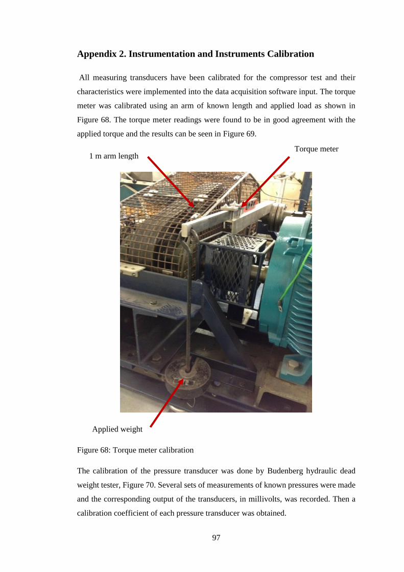
97

Appendix 2. Instrumentation and Instruments Calibration

All measuring transducers have been calibrated for the compressor test and their

characteristics were implemented into the data acquisition software input. The torque

meter was calibrated using an arm of known length and applied load as shown in

Figure 68. The torque meter readings were found to be in good agreement with the

applied torque and the results can be seen in Figure 69.

Figure 68: Torque meter calibration

The calibration of the pressure transducer was done by Budenberg hydraulic dead

weight tester, Figure 70. Several sets of measurements of known pressures were made

and the corresponding output of the transducers, in millivolts, was recorded. Then a

calibration coefficient of each pressure transducer was obtained.

Torque meter

Applied weight

1 m arm length

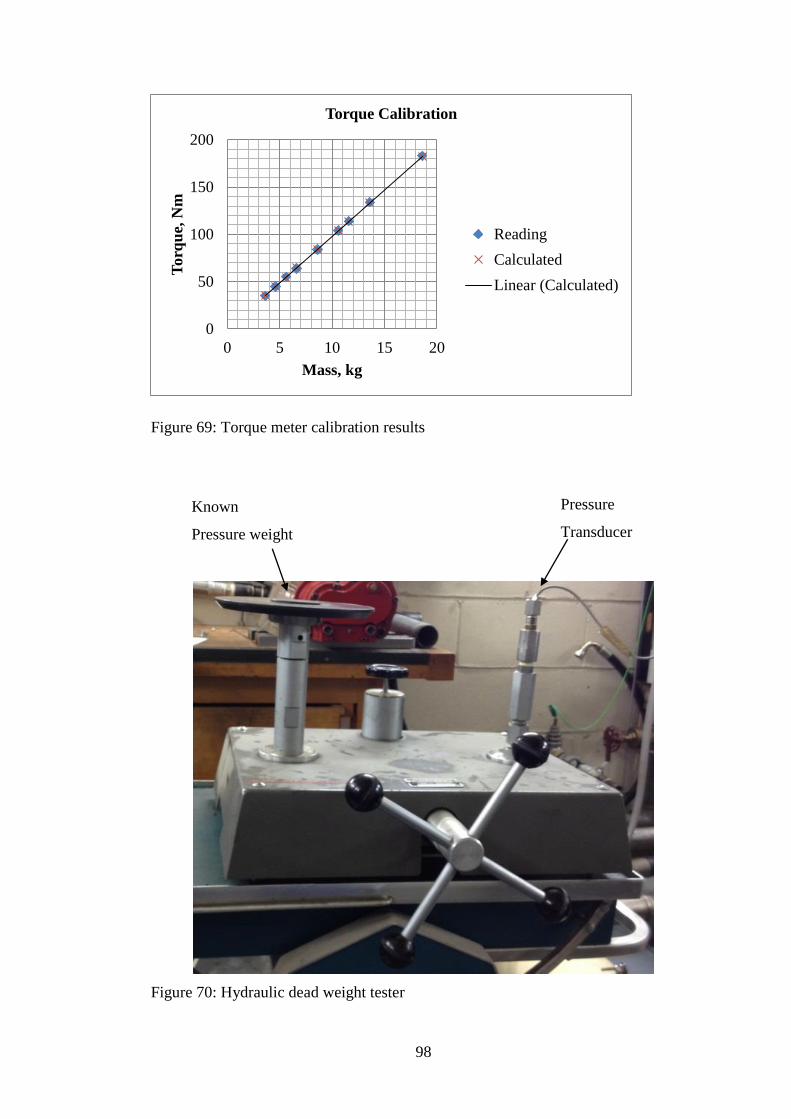
98

Figure 69: Torque meter calibration results

Figure 70: Hydraulic dead weight tester

0

50

100

150

200

0 5 10 15 20

Torq

ue,

Nm

Mass, kg

Torque Calibration

Reading

Calculated

Linear (Calculated)

Pressure

Transducer

Known

Pressure weight

99

The digital tachometer on the shaft of the compressor was verified with an optical

tachometer and both readings were found to be in good agreement with each other.

Where appropriate the K-type thermocouples were verified with either a mercury or

infrared thermometer.

Table 10 below gives the list of installed instruments used for measurement the

operating parameters of a compressor.

Table 10: Description of the test rig instruments

Measured

Parameter

Instrument Specifications

Compressor

Speed, n

Tachometer

(RPM transducer)

6 0 TTL pulses per revolution,

Accuracy= 0.1%

Compressor

Torque, M

TRP-500 torque meter

(strain gauge transducer)

max torque: 500Nm, Calibration

level: 335Nm Range = 0 - 6000 rpm,

Supply volt=10v dc, Accuracy= 0.25 %

of max torque

inlet pressure, p PDCR 110/w -pressure

transducer

(piezoresistive type)

Operating range = 3.5bar(abs)

Excite voltage=10V dc, Accuracy

=0.6%,

inlet

temperature , T1

K- type thermocouple

(based on Ni/Cr-Ni/Al alloy )

Range= -2000C to 13000C, Accuracy=

2.20C sensitivity = 41 µV/°C

outlet pressure,

p

PDCR 922-pressure

transducer

(piezoresistive type)

Operating range =15 bar (abs)

Excite voltage=10V dc, Output

voltage= 100 mV Accuracy =0.6%

outlet

temperature, T2

K- type thermocouple

(based on Ni/Cr-Ni/Al )

Range= -2000C to 13000C,

Accuracy= 2.20C sensitivity = 41

µV/°C

100

Appendix 3. Data Acquisition and processing

All the data from the transducers were collected by a data acquisition system. It

consists of a National Instrument Compact-RIO, CRIO-9022 Real-Time with an 8

slots chassis CRIO-9114. It has an industrial 533 MHz real-time processor for reliable

real-time applications. Compact _RIO has 256 MB of DDR2 RAM and 2 GB of non-

volatile storage for holding programs and logging data. The unit also permits the

acquisition of signals from the measurement transducers simultaneously during the

experiment that are inputs to the unit itself and connected to a computer via an Ethernet

cable. The programming was done using LabVIEW Field Programmable Gate Array

which is suitable for high frequency data acquisition. The measurements obtained

from the transducers are acquired on the CRIO and send to the PC which is

programmed to instantaneously calculate values of the compressor power

consumption, air flow rate, specific quantities and efficiency. All required information

is displayed on a computer monitor in real time as presented in Figure 4 and Figure 6.

Measurement records were collected twice a second and saved in a separate file which

was used for further analysis. Before the measurements, the compressor and its plant

were run for 30 minutes to obtain steady temperature in the compressor casing and to

bring the oil temperature to its working level.

101

Appendix 4. Reynolds Transport Theorem

Reynolds Transport Theorem defines a change of variable in a control volume V

limited by area A which vector of local normal is dA and which travels at local speed

v. This control volume may, but not necessarily coincides with the engineering or

physical material system. The rate of change of variable in time within the volume

is:

V V

dVt t

(1)

Therefore, it may be concluded that the change of variable in the volume V is caused

by:

- change of the specific variable =/m in time within the volume because of

sources (and sinks) in the volume, dVt

which is called a local change and

- the movement of the control volume which takes new space with variable in

it and leaves old space, causing a change in time of for v.dA and which is

called convective change.

The first contribution may be represented by a volume integral:

V

dVt

(2)

while the second contribution may be represented by a surface integral:

A

d v A (3)

Therefore:

V V V A

ddV dV d

t dt t

v A (4)

which is a mathematical representation of Reynolds Transport Theorem.

Applied to a material system contained within the control volume Vm which has

surface Am and velocity v which is identical to the fluid velocity w, Reynolds

Transport Theorem reads:

102

Vm Vm Vm Am

ddV dV d

t dt t

w A (5)

If that control volume is chosen in one moment to coincide with the control volume

V, the volume integrals are identical for V and Vm and the surface integrals are

identical for A and Am, however, the time derivatives of these integrals are different,

because the control volumes will not coincide in the next time interval. However, there

is a term which is identical for the both times intervals:

V Vm

dV dVt t

(6)

therefore,

Vm VAm A

d dt t

w A v A (7)

or:

Vm V A

dt t

w v A (8)

If the control volume is fixed in the coordinate system, i.e. if it does not move, v=0

and consequently:

V V

dVt t

(9)

therefore:

Vm V A

dV dt t

w A (10)

Finally application of Gauss theorem leads to the common form:

Vm V V

dV dVt t

w (11)

103

As stated before, a change of variable is caused by the sources q within the volume

V and influences outside the volume. These effects may be proportional to the system

mass or volume or they may act at the system surface. The first effect is given by a

volume integral and the second effect is given by a surface integral.

V A V A

Vm Vm Am V V

q dV q d q q dV qdVt

A (12)

q can be scalar, vector or tensor.

A combination of the two last equations gives:

or

0

V A V

V

dV d qdVt

q dVt

w A

w

(13)

Omitting integral signs gives:

0qt

w (14)

This is well known conservation law form of variable . Since for =1, this

becomes continuity equation: 0t

w finally it is:

0 orqt t

Dq

dt t

w w

w

(15)

D/dt is the material or substantial derivative of variable. This equation is very

convenient for derivation of particular conservation laws. As previously mentioned

=1 leads to continuity equation, =u to momentum equation, =e, where e is specific

internal energy, leads to energy equation, =s, to entropy equation and so on.

If the surfaces where fluid carrying variable goes into or exits from the control

volume can be identified, a convective change may conveniently be written:

104

in outin out

A

d dm m m w A (16)

where bar denotes the variable average at entrance/exit surface sections. This leads to

macroscopic form of the conservation law:

in out in outV V

ddQ m m Q

dt dt

(17)

which states in words: (rate of change of )=(inflow )-(outflow )+(source of )

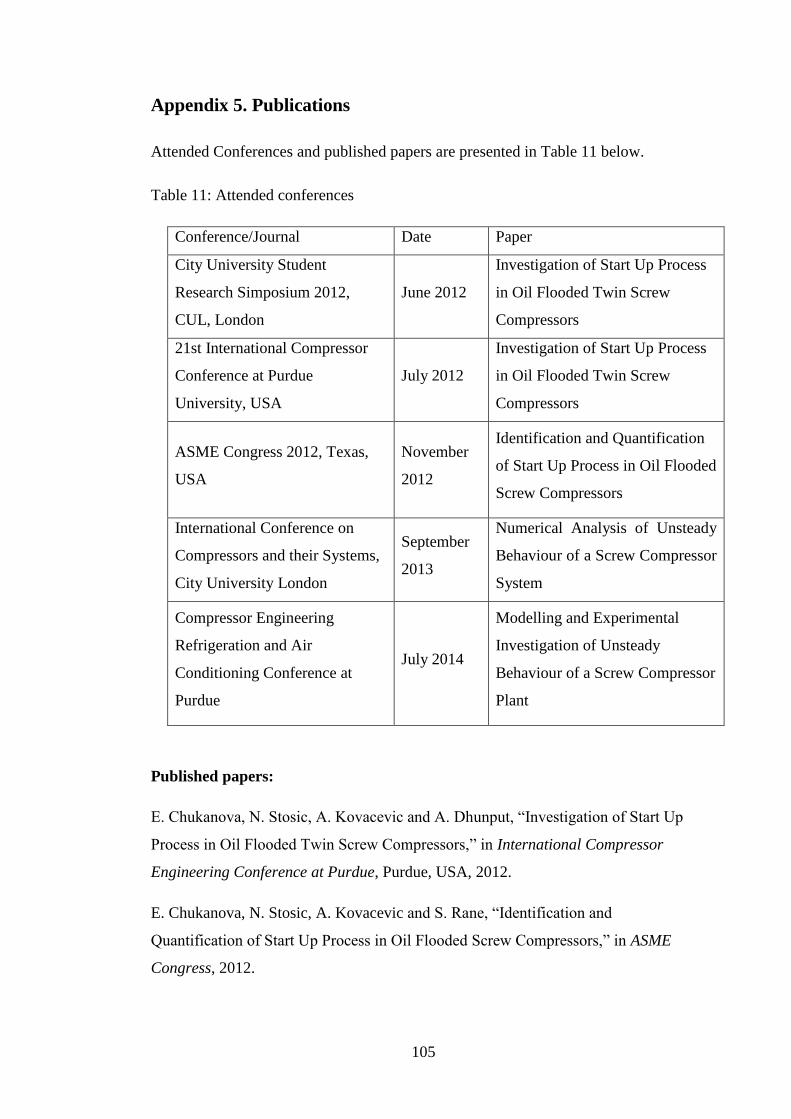
105

Appendix 5. Publications

Attended Conferences and published papers are presented in Table 11 below.

Table 11: Attended conferences

Conference/Journal Date Paper

City University Student

Research Simposium 2012,

CUL, London

June 2012

Investigation of Start Up Process

in Oil Flooded Twin Screw

Compressors

21st International Compressor

Conference at Purdue

University, USA

July 2012

Investigation of Start Up Process

in Oil Flooded Twin Screw

Compressors

ASME Congress 2012, Texas,

USA

November

2012

Identification and Quantification

of Start Up Process in Oil Flooded

Screw Compressors

International Conference on

Compressors and their Systems,

City University London

September

2013

Numerical Analysis of Unsteady

Behaviour of a Screw Compressor

System

Compressor Engineering

Refrigeration and Air

Conditioning Conference at

Purdue

July 2014

Modelling and Experimental

Investigation of Unsteady

Behaviour of a Screw Compressor

Plant

Published papers:

E. Chukanova, N. Stosic, A. Kovacevic and A. Dhunput, “Investigation of Start Up

Process in Oil Flooded Twin Screw Compressors,” in International Compressor

Engineering Conference at Purdue, Purdue, USA, 2012.

E. Chukanova, N. Stosic, A. Kovacevic and S. Rane, “Identification and

Quantification of Start Up Process in Oil Flooded Screw Compressors,” in ASME

Congress, 2012.

106

E. Chukanova, N. Stosic, A. Kovacevic, “Numerical Analysis of Unsteady

Behaviour of a Screw Compressor System,” in International Conference on

Compressors and their Systems, City University London, 2013.

E. Chukanova, N. Stosic , A. Kovacevic (2013). Experimental Investigation and

Numerical Modelling of Dynamic Behaviour of Screw Compressor Plant. Universal

Journal of Engineering Science, 1 , 68 - 79.

E. Chukanova, N. Stosic, A. Kovacevic, “Modelling and Experimental Investigation

of Unsteady Behaviour of a Screw Compressor Plant” in International Compressor

Engineering Conference at Purdue, Purdue, USA, 2014.

E. Chukanova, N. Stosic, A. Kovacevic, “Verification and Calibration of Dynamic

Model of Screw Compressor Plant” in ASME Congress, 2015.

city research onlineopenaccess.city.ac.uk/15825/1/chukanova, ekaterina.pdf · 6 figure 20:...

Documents