city research onlineopenaccess.city.ac.uk/2381/1/osborne,_matthew.pdf · urls from city research...
TRANSCRIPT

City, University of London Institutional Repository
Citation: Osborne, Matthew (2013). Essays on bank capital and balance sheet adjustment in the UK and US, and implications for regulatory policy. (Unpublished Doctoral thesis, City University London)
This is the unspecified version of the paper.
This version of the publication may differ from the final published version.
Permanent repository link: http://openaccess.city.ac.uk/2381/
Link to published version:
Copyright and reuse: City Research Online aims to make research outputs of City, University of London available to a wider audience. Copyright and Moral Rights remain with the author(s) and/or copyright holders. URLs from City Research Online may be freely distributed and linked to.
City Research Online: http://openaccess.city.ac.uk/ [email protected]
City Research Online
Essays on bank capital and balance sheet adjustment in
the UK and US, and implications for regulatory policy
Matthew Edward Osborne
Supervisors:
Professor Ana-Maria Fuertes
(Cass Business School, City University, London)
Professor Alistair Milne
(Loughborough University School of Business and Economics)
A thesis submitted for the degree of Doctor of Philosophy
Faculty of Finance, Cass Business School, City University, London
July 2012

ii
This page is intentionally left blank.

iii
Table of contents
Table of contents ................................................................................................. iii
List of tables ........................................................................................................vii
List of figures ....................................................................................................... ix
Acknowledgements .............................................................................................. xi
Declaration ........................................................................................................ xiii
Abstract of thesis ................................................................................................. xv
Chapter 1 : Introduction ...................................................................................... 1
1.1 Motivation ........................................................................................................................ 1
1.2 Summary of contributions made by the thesis ................................................................. 5
Chapter 2 : Literature Review .......................................................................... 10
2.1 Theories of capital structure ........................................................................................... 10
2.1.1 Trade-off theory: taxes and bankruptcy costs.......................................................... 13
2.1.2 Information costs and the pecking order theory ...................................................... 15
2.1.3 Whether banks are ―special‖ and how this affects the capital structure .................. 17
2.2 How bank capital may affect the supply of credit to the economy ................................ 24
2.2.1 The bank capital channel ......................................................................................... 24
2.2.2 The bank lending channel ........................................................................................ 28
2.3 Literature on the relationship between bank capital and interest margins ..................... 30
2.3.1 Theories on the long-run relationship between bank capital and interest margins . 31
2.3.2 Theories on the short run relationship between bank capital and margins .............. 35
2.3.3 Bank capital, portfolio risk and interest margins ..................................................... 36
Chapter 3 : Capital requirements and bank behaviour in the UK..................... 40
3.1 Introduction .................................................................................................................... 40
3.2 Literature Review and background on UK banking sector ............................................ 44
3.2.1 Review of literature on bank capital requirements and bank behaviour ................. 44
3.2.2 Background on the UK banking sector .................................................................... 47
3.3 Framework for evaluating the impacts of capital requirements ..................................... 53
3.3.1 The target capital ratio model .................................................................................. 53
3.3.2 The measure of bank capitalization ......................................................................... 57

iv
3.3.3 The effects of bank capitalization on balance sheet and lending growth ................ 57
3.4 Data and description of sample ...................................................................................... 61
3.5 Empirical results ............................................................................................................. 64
3.5.1 Bank capital ratio ..................................................................................................... 64
3.5.2 Bank balance sheet adjustment ................................................................................ 66
3.6 Policy implications ......................................................................................................... 70
3.7 Extension to the crisis period ......................................................................................... 76
3.8 Conclusions .................................................................................................................... 83
Chapter 4 : In Good Times and in Bad: Bank Capital Ratios and Lending
Rates 86
4.1 Introduction .................................................................................................................... 86
4.2 The interrelationship of bank capital and loan interest rates .......................................... 89
4.2.1 Conceptual and theoretical background .................................................................. 89
4.2.2 Previous empirical studies of bank capital and loan interest rates .......................... 96
4.3 Methodology, Data and Variables ................................................................................ 100
4.3.1 Empirical strategy .................................................................................................. 103
4.3.2 Description of data and variables .......................................................................... 100
4.4 Empirical results ........................................................................................................... 109
4.4.1 Descriptive statistics .............................................................................................. 109
4.4.2 Tests of hypothesis on the relation between capital ratio and loan rates ............... 113
4.5 Conclusions and implications....................................................................................... 120
Chapter 5 : Capital and profitability in banking: Evidence from US banks... 124
5.1 Introduction .................................................................................................................. 124
5.2 Literature review .......................................................................................................... 130
5.2.1 Theory and evidence on the relation between capital and profitability in banks .. 130
5.2.2 Trends in capital and profitability of US banking sector, 1976-2010 ................... 135
5.3 Extending the results of Berger (1995) ........................................................................ 142
5.3.1 Data and specification ........................................................................................... 143
5.3.2 Results ................................................................................................................... 147
5.3.3 Problems with the model based on Berger (1995) ................................................ 150
5.4 Towards an improved model of capital and profitability ............................................. 153
5.4.1 Specification .......................................................................................................... 155
5.4.2 Results ................................................................................................................... 160

v
5.5 Conclusions .................................................................................................................. 175
Chapter 6 : Conclusion ................................................................................... 199
References ......................................................................................................... 203

vi
This page is intentionally left blank.
vii
List of tables
Table 3.1: International claims of the UK financial services sector, 2007 .............................. 52
Table 3.2: Descriptive statistics for the variables in our analysis ............................................ 63
Table 3.3: Estimation of long-run target capital ratio .............................................................. 65
Table 3.4: Determinants of growth in balance sheet components, 1996Q1 - 2007Q4 ............ 67
Table 3.5: Simulation of effects of 3 percentage point increase in capital requirements ........ 73
Table 3.6: Summary statistics for variables in analysis, big banks only ................................. 81
Table 3.7: Determinants of growth of balance sheet components 1996Q1-2011Q2 ............... 83
Table 4.1. Summary statistics for bank-specific covariates in loan pricing ECM equation. . 112
Table 4.2. Estimation of loan interest rate ECM equation 1998:10-2011:06. ....................... 117
Table 5.1: Descriptive statistics for control variables, 1977-2010 ........................................ 147
Table 5.2: Descriptive statistics for size and risk groups ...................................................... 157
Table 5.3: Long-run target capital structure, groups 1-3 (small banks)................................. 162
Table 5.4: Long-run target capital structure, groups 4-6 (medium-sized banks) ................... 163
Table 5.5: Long-run target capital structure, groups 7-9 (big banks) .................................... 164

viii
This page is intentionally left blank.

ix
List of figures
Figure 3.1: Risk-weighted capital ratio and lending/GDP ratio, 1990-2007 .......................... 50
Figure 3.2: Risk-weighted capital ratios and supervisory capital requirements ...................... 54
Figure 3.3: Distribution of estimated Zit over time ................................................................. 64
Figure 3.4: Simulation of effects of 3 percentage point increase in capital requirements ....... 74
Figure 3.5: Tier 1 capital ratio for all banks, 1989Q4-2011Q2 ............................................... 78
Figure 3.6: Total and tier 1 risk-weighted capital ratios and total capital requirements, big and
small banks, 2007Q1-2011Q2 ................................................................................................. 79
Figure 4.1. Illustration of long-run cost of capital curve. ........................................................ 91
Figure 4.2: Illustration of short-run relation between capital and interest margins ................. 95
Figure 4.3: Trends in UK capital ratios and lending rate. ...................................................... 110
Figure 4.4. CDS indices for banks in the sample. .................................................................. 111
Figure 4.5. Coefficients on time dummies from estimation of target capital ratio. .............. 115
Figure 4.6. Illustration of short- and long-run effects of capital ratio on lending rates in crisis.
................................................................................................................................................ 119
Figure 5.1: Descriptive statistics on US commercial banks' capital-asset ratio and return on
equity, 1976-2010, all banks .................................................................................................. 137
Figure 5.2: Descriptive statistics on US commercial banks' capital-asset ratio and return on
equity, 1976-2010, large banks .............................................................................................. 138
Figure 5.3: FDIC bank failures 1976-2010 ............................................................................ 142
Figure 5.4: Estimated effect of k on ROE 1977-2010 ........................................................... 149
Figure 5.5: Charts of median k and median k* , and buffer at the 10th, 25th, 75th and 90th
percentiles .............................................................................................................................. 165
Figure 5.6: Coefficients on capital variables in regression of ROA ...................................... 172

x
This page is intentionally left blank.

xi
Acknowledgements
In writing this thesis, I have been given very helpful assistance by my supervisors, Professors
Ana-Maria Fuertes (Cass Business School) and Alistair Milne (Loughborough University
School of Business and Economics). Professor Milne was initially my lead supervisor, and I
am very grateful to him for his support and belief in me at the start of my PhD when I was
unsure whether it would be possible to combine a research degree with my work in the policy
area of the Financial Services Authority. Professor Milne has helped with theoretical
discussion throughout the thesis. Professor Fuertes made a detailed contribution to the
econometric methods.
I would also like to thank members of the Faculty of Finance at Cass Business School for
helpful support and comments throughout the course of the PhD, and Malla Pratt and Abdul
Momin in the PhD Office for administrative support.
I would like to dedicate this thesis to my wife Anushka, without whose love, patience and
support it would not have been possible.

xii
This page is intentionally left blank.

xiii
Declaration
I grant powers of discretion to the university librarian to allow this thesis to be copied in
whole or in part without further reference to me. This permission covers only single copies
made for study purposes, subject to normal conditions of acknowledgment.

xiv
This page is intentionally left blank.

xv
Abstract of thesis
The financial crisis prompted widespread interest in developing a better understanding of
how market and regulatory driven capital targets affect bank behaviour. Such considerations
are important to assessing the effects of shocks to banks' capital ratios on their supply of
financial intermediation services to the real economy, whether those shocks originate in
higher regulatory capital requirements, unexpected losses, or demands from investors or
counterparties. In particular, my research is relevant to the effects of changes in capital
requirements or the imposition of explicitly counter-cyclical capital requirements, as
proposed by the Basel III agreement. In this thesis, I describe three related research chapters
focusing on how banks' actual capital ratios and long-run capital ratio targets affect bank
behaviour.
The first chapter uses a unique, comprehensive database of regulatory capital requirements on
all UK banks to examine their effects on capital, lending and balance sheet management
behaviour in the pre-crisis period 1996-2007. We find that capital requirements that include
firm-specific, time-varying add-ons set by supervisors affect banks‘ desired capital ratios and
that resulting adjustments to capital and lending depend on the gap between actual and target
ratios. We use these results to measure the effects of a capital regime that includes features
similar to those embedded in the UK framework. Our results suggest that countercyclical
capital requirements may be less effective in slowing credit activity when banks can readily
satisfy them with lower-quality (lower-costing) capital elements versus higher-quality
common equity. Finally, we apply a simple version of our model to a small sample of large
banks in the crisis period 2007-2011 and find that balance sheet adjustments to achieve target
tier 1 capital ratios focused on risk-weighted assets, and changes in tier 1 and total capital
played a reduced role compared to the pre-crisis period. Given the size of the UK banking
sector and the global nature of many of the largest institutions in the UK banking sector, the
results have implications for the ongoing debate surrounding the design and calibration of
international capital standards.
The second chapter assesses the relation between bank capital ratios and lending rates for the
8 largest UK banks over the period 1998-2011. The methods differ from previous literature in
that they employ a dynamic error correction specification and a unique regulatory database to
disentangle long- and short-run effects. There is no long-run link in pre-crisis boom times,
xvi
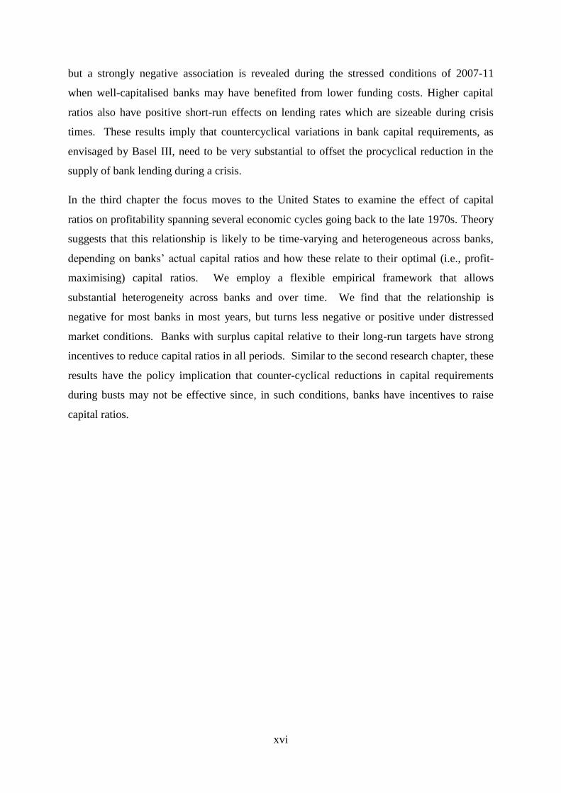
but a strongly negative association is revealed during the stressed conditions of 2007-11
when well-capitalised banks may have benefited from lower funding costs. Higher capital
ratios also have positive short-run effects on lending rates which are sizeable during crisis
times. These results imply that countercyclical variations in bank capital requirements, as
envisaged by Basel III, need to be very substantial to offset the procyclical reduction in the
supply of bank lending during a crisis.
In the third chapter the focus moves to the United States to examine the effect of capital
ratios on profitability spanning several economic cycles going back to the late 1970s. Theory
suggests that this relationship is likely to be time-varying and heterogeneous across banks,
depending on banks‘ actual capital ratios and how these relate to their optimal (i.e., profit-
maximising) capital ratios. We employ a flexible empirical framework that allows
substantial heterogeneity across banks and over time. We find that the relationship is
negative for most banks in most years, but turns less negative or positive under distressed
market conditions. Banks with surplus capital relative to their long-run targets have strong
incentives to reduce capital ratios in all periods. Similar to the second research chapter, these
results have the policy implication that counter-cyclical reductions in capital requirements
during busts may not be effective since, in such conditions, banks have incentives to raise
capital ratios.
1
Chapter 1 : Introduction
Regulatory capital requirements imposed on banks have acquired a new importance as a
result of the global financial crisis which began in 2007 and still continues today. However,
the benefits of higher capital requirements, in terms of a reduced likelihood of bank failure
and systemic distress, need to be carefully weighed against the costs of reduced supply of
credit to the real economy. In this thesis, I examine several research questions which are
relevant to the consideration of the impact of higher capital requirements for banks, and also
to the operation of capital requirements with specifically counter-cyclical aims. First, I ask
whether capital requirements are a significant factor in the determination of banks' own
choice of capital ratio, and if so, how banks adjust their balance sheets in order to achieve
their targeted buffer over the required minimum. This is particularly relevant to assessing the
economic impact of higher capital requirements, since banks may respond to a deficit of
capital by reducing the supply of credit to the real economy. Second, I examine the
relationship between banks' capital ratios and their lending interest rates, specifically whether
the short-run effects different from the long-run effects and the extent to which the
relationship may vary or change sign depending on conditions in the banking sector. Finally,
I ask under what conditions a higher capital ratio may increase a bank's profitability, and
when it may decrease profitability. These second and third questions are important to
understanding the potential effects of a counter-cyclical capital requirement, since they shed
light on the interaction of capital requirements with the private incentives banks may have to
raise or lower capital ratios.
1.1 Motivation
One factor that has been prominent in accounts of the financial crisis that gripped world
markets in 2007-09 is that capital ratios in developed countries became low by historical
standards by the late 1990s and early 2000s (Berger et al, 1995; Bank of England, 2009) and
once the scale of the losses arising from sub-prime lending and associated structured credit
products became clear, markets lost confidence in many large banks‘ ability to absorb these
2
losses and remain going concerns (Milne, 2009; FSA, 2009). The perception that regulatory
capital standards for banks were set too low has played a key role in accounts of the crisis by
the European Commission, the Basel Committee on Banking Supervision (BCBS), the UK
Financial Services Authority (FSA), and the Organisation for Economic Cooperation and
Development (OECD), and it has been accompanied by calls for tighter regulation of capital
and liquidity in future.1 For example, the declaration made by the G20 after the Washington
summit following the failure of Lehman Brothers in November 2008 stated:
―Policy-makers, regulators and supervisors, in some advanced countries, did not
adequately appreciate and address the risks building up in financial markets, keep
pace with financial innovation, or take into account the systemic ramifications of
domestic regulatory actions. (…) We pledge to strengthen our regulatory regimes,
prudential oversight, and risk management, and ensure that all financial markets,
products and participants are regulated or subject to oversight, as appropriate to their
circumstances.‖
and the Action Plan from that summit included a commitment to:
―Ensure that firms maintain adequate capital, and set out strengthened capital
requirements for banks' structured credit and securitization activities.‖
At the same time, central banks and regulators around the world are considering how
regulatory tools would be used to achieve so-called ―macro-prudential‖ policy objectives in
which regulation aims to smooth credit cycles by constraining credit growth during booms
and stimulating new lending during busts. The Basel III agreement includes a requirement
that supervisors should vary capital buffers procyclically:
―The Basel Committee is introducing a regime which will adjust the capital buffer
range, established through the capital conservation mechanism outlined in the
previous section, when there are signs that credit has grown to excessive levels. The
1 See Blundell-Wignall, A., Atkinson, P. and Lee, S. H. (2008), The Current Financial Crisis: Causes and Policy
Issues, OECD Financial Market Trends; European Commission (2009), Economic Crisis in Europe: Causes,
Consequences and Responses, European Economy 7; Bank for International Settlements, 2008 Annual Report;
and FSA (2009), The Turner Review: A Regulatory Response to the Crisis.
3
purpose of the countercyclical buffer is to achieve the broader macroprudential goal
of protecting the banking sector in periods of excess aggregate credit growth.‖ 2
These proposals are in the first stages of implementation by supervisors. At the time of
writing, counter-cyclical capital requirements which can be varied by national supervisors are
included in the draft implementation of Basel III in the European Union, and the Bank of
England has published its initial views on the operation of such macroprudential tools (Bank
of England, 2011).
However, though the benefits of tighter prudential standards could not be clearer following
the events of 2007-08, some existing research evidence suggests that higher capital
requirements may suppress credit growth, with potentially harmful consequences for
economic growth (see, e.g. Berger and Udell, 1994; Thakor, 1996; Berrospide and Edge,
2010; Francis and Osborne, 2009).3 A heated debate is underway between those who believe
that capital requirements impose minimal costs on banks due to the Modigliani-Miller
Theorems (see, e.g., Admati et al, 2009) and the views of some regulated firms who believe
that equity capital is relatively costly.4 Therefore, in order to be effective and proportionate,
the design and calibration of regulation needs to be based on evidence about the incremental
impact of voluntary and involuntary changes in capital on bank behaviour. This is the subject
of a substantial existing academic literature, and several early attempts have been made to
assess the costs and benefits of higher prudential standards following the recent financial
crisis (Barrell et al, 2009; Kato et al, 2010; Miles et al, 2011; Institute for International
Finance, 2011; see Basel Committee, 2010 for a good review).
An important theoretical insight is that the effect of capital requirements on bank behaviour
depends on the extent to which banks have incentives to hold higher capital than the regulator
requires. This excess capital could be a precautionary buffer against breaching the regulatory
minimum (see, e.g., Estrella, 2004; Milne and Whalley, 2002; Peura and Keppo, 2006),
implying that changes in capital requirements will change the capital ratios chosen by banks.
However, it could also be that banks themselves have incentives to hold high levels of capital
2 Basel Committee on Banking Supervision (June 2011) Basel III: A global regulatory framework for more
resilient banks and banking systems, p. 7. 3 It is worth pointing out even at this early stage that the literature on whether capital requirements caused the
early 1990s ―credit crunch‖ is mixed; see Chapter 2. 4 Such comment has been fairly ubiquitous in the financial press; for one notable example see Pandit, V. (2010),
―We must rethink Basel III or growth will suffer‖, Financial Times, November 2010.
4
due to market pressures to control overall bank risk (Berger, 1995; Flannery and Rangan,
2008; Berger et al, 2008), and hence it could be the case that capital requirements do not
affect banks‘ choice of capital ratio at all.
In the latter case, it is questionable whether changes in capital requirements would have much
effect at all on bank behaviour, at least at the margin, since it is the bank‘s own private
optimal capital ratio that determines actual capital holdings. Clearly, the effect of capital
requirements depends strongly on how they interact with banks‘ own capital targets,
sometimes called ―market capital requirements‖, which are sometimes substantially in excess
of regulatory capital requirements. These internal optimal capital ratios may be determined
by factors studied in more conventional corporate finance theory, such as the popular ―trade-
off‖ theory of capital structure, as well as those factors which are particularly relevant for
banks. Furthermore, since banks‘ optimal ratios are likely to depend on the probability of
default they are likely to be strongly cyclical, and banks will target much higher capital ratios
in periods of financial distress (Berger, 1995).
These insights suggest that the response of banks to changes in capital requirements varies
not only depending on how high capital requirements are set, but also on the level of capital
that banks themselves would choose in the absence of regulation. Intuitively, for a bank that
wishes to hold 5%, a capital requirement change from 10% to 9% will reduce the cost of
regulation for the bank. Now consider if the bank‘s own optimal capital ratio increases to
10%, due to stressed market conditions and the need to reassure investors of its solvency. If
the regulator repeats the policy change and reduces capital requirements from 9% to 8%, this
would have no effect on the bank‘s behaviour since due to market incentives the bank must
now hold capital in excess of the capital requirement. These considerations are important to
the design of counter-cyclical capital requirements, since this tool aims to reduce banks‘
capital ratios under stressed conditions in order to stimulate new lending. Their efficacy
depends on the idea that regulatory capital requirements continue to bind banks under stress,
and therefore on the extent to which regulatory and market capital requirements interact with
each other.
In Chapter 2, I have included a literature review of fundamental aspects of corporate finance
and banking research relevant to the thesis. In particular, this reviews basic theories of
capital structure; the extent to which banks may be different to other firms in their choice of
capital structure; how bank capital affects bank behaviour and macroeconomic outcomes; and
5
theory on the link between bank capital and interest margins. Each of the three research
chapters also has its own literature review which covers more specialised and recent literature
relevant to their respective research questions.
1.2 Summary of contributions made by the thesis
In this thesis I present new evidence on the effect of regulatory and market capital targets on
bank behaviour.5 Our research examines three related elements of the behavioural and
market impact of bank capital targets. The first research chapter focuses on how regulatory
targets affected banks‘ balance sheet management during a period in which capital
requirements were binding on UK banks. The second and third chapters focus on the
cyclicality of optimal bank capital, and assess the idea that capital targets will have a very
different effect on bank behaviour ―in good times and in bad‖. Below I note the empirical
contributions of each chapter in turn.
The first research chapter (Chapter 3) is a detailed analysis of how banks adjusted
components of their balance sheets in response to supervisory specified, bank- and time-
specific capital requirements in the UK. A significant drawback of previous literature that
claims to identify the effect of capital requirements based on banks relatively close to the
minimum is that such effects are difficult to distinguish from what we would expect from low
capital banks in the absence of capital requirements (e.g. Jackson et al, 1999; Sharpe, 1995;
Berrospide and Edge, 2010; Osterberg and Thomson, 1996; Gropp and Heider, 2010). The
reason for this is that under the regulatory regime established by the Basel Accord, different
banks tend to be subject to the same capital requirement, which makes it impossible to
compare the response of a bank which is constrained by the capital requirement with the
response of another bank which has the same capital ratio but is not similarly constrained.
This chapter uses a unique, comprehensive database of regulatory capital requirements on
UK banks over the period 1996-2007, including firm-specific, time-varying add-ons set by
supervisors, to examine their effects on capital, lending and balance sheet management
5 The author is an employee of the FSA, and is therefore uniquely placed to examine these questions, given
access to confidential in-house data on UK banks and contacts in the regulatory and central banking community.
My intention is that this work will be influential in assessing the likely effects of proposed prudential policy
reform.

6
behaviour. These add-ons are invisible to the market and therefore allow us to identify the
incremental effect of capital requirements. I find that banks‘ capital targets are significantly
associated with capital requirements, and that management of assets and liabilities is strongly
influenced by the difference between target and actual capital. Banks that are below (above)
their targets tend to have higher (lower) capital growth and lower (higher) asset growth.
Furthermore, the adjustment of assets tends to focus on those with a higher regulatory risk
weight, while the adjustment of capital focuses is larger for lower quality regulatory tier 2
capital than for the relatively more costly but higher quality tier 1 capital. These findings are
consistent with the interpretation that these adjustments are driven by the regulatory regime
rather than banks‘ own incentives. As an additional robustness check, I isolate those
observations for which banks‘ targets have changed due to changes in capital requirements,
and find that the response is even more skewed towards tier 2 capital and higher risk-
weighted assets. Our results suggest that countercyclical capital requirements may be less
effective in slowing credit activity when banks can readily satisfy them with lower-quality
(and lower-cost) capital elements versus higher-quality common equity.
The second research chapter (Chapter 4) considers the role of capital in determining lending
rates. While there have been a large number of empirical studies of this relationship in the
past (Carbó-Valverde and Rodríguez-Fernández, 2007; Saunders and Schumacher, 2000;
Demirgüç-Kunt and Huizinga, 1999; Santos and Winton, 2010; Steffen and Wahrenburg,
2008; Hubbard et al, 2002), these studies suffer from the drawback that they do not allow the
relationship to vary over time, and they do not separate out the long-run and short-run
relationship between capital and lending rates. I argue that it is crucial to allow for these
features of the relationship since the direction may actually reverse in the long run and the
short run, and in distressed and non-distressed periods. This may explain the fact that the
above studies are split between those that find a positive or a negative relationship.
This chapter assesses the relation between bank capital ratios and lending rates for the 8
largest UK banks over the period 1998-2011. Our paper differs from previous literature in
that I employ a dynamic error correction specification (based on Fuertes et al, 2009) and a
unique regulatory database to disentangle long- and short-run effects, and I allow the
relationship to vary over pre-crisis (―good times‖) and crisis (―bad times‖). There is no long-
run link in pre-crisis boom times, but a strongly negative association is revealed during the
stressed conditions of 2007-11 when well-capitalised banks may have benefited from lower
funding costs. Higher capital ratios also have positive short-run effects on lending rates which

7
are sizeable during crisis times. Given the size of the UK banking sector and the global
nature of many of the largest institutions in the UK banking sector, the results have
implications for the ongoing debate surrounding the design and calibration of international
capital standards. The results imply that countercyclical variations in bank capital
requirements, as envisaged by Basel III, may need to be very substantial to offset the
procyclical reduction in the supply of bank lending during a crisis.
The third and final research chapter (Chapter 5) turns to the US in order to analyse how the
relationship between bank capital and profitability varies over financial cycles. This chapter
is relatively preliminary compared to the first two since there remain some technical
challenges to be overcome. Suggestions from the examiners on improvements to the
methodology would be very welcome. An important paper to have examined the relationship
between capital and earnings was Berger (1995), which found that the effect of capital on
banks‘ profitability was negative in the period 1983-89 when the banking sector was under
stress (the ―savings and loan crisis‖) and positive in the early 1990s when banks‘ capital
ratios had recovered and indeed been boosted by new capital requirements. I revisit these
findings in order to apply the conceptual framework of ―in good times and in bad‖ developed
in Chapter 4 to the US banking market, which is very different from the UK due to its large
size and diversity. A significant advantage of examining the US is the availability of a very
large dataset of US banks; our sample has up to 15,000 banks over 30 years, over 1.6 million
bank-quarter observations in total. This allows for substantial heterogeneity and robust
estimation over several financial cycles.
The contributions of this chapter are in two parts. In the first part of the chapter I extend the
results of Berger (1995) to assess whether capital ratios ―Granger cause‖ banks‘ return on
equity. The main contributions to the literature are that I estimate the model in a systematic
manner over a much longer time period than the original study, and I show that the results are
robust to the use of more recent and sophisticated econometric techniques. I extend the
original sample period (1983-92) to include data up to 2010 spanning the recent financial
crisis. I find an upswing in the relationship between capital and ROE in the recent market
stress, although this is lesser in magnitude compared to the upswing observed by Berger for
the 1983-89 period. This is consistent with the idea of "In good times and in bad" that in
periods of distress, banks may improve their profitability by increasing their capital ratios.
8
However, the original specification on which the analysis is based has a number of flaws,
chief among which is the possible reverse causality from profits to capital which is not fully
captured by the reduced form model used by Berger (1995). Therefore, in the second part, I
present the results of an initial attempt to deal with some of these issues. The contribution of
this analysis to the literature is that we apply the concept of a long-run target capital ratio to
US banks and use this to examine the short-run effect of deviations from the optimal capital
ratio. We estimate target capital ratios using a similar method to Chapter 3 and Chapter 4,
and then model the return on assets allowing the relationship between capital and profitability
to vary depending on whether banks are above or below their target capital ratio. We find
long-run positive co-movement of profits and capital ratios, and furthermore we find an
asymmetry in the effect of deviations from the long-run target capital ratio; banks that are
above the long-run target capital ratio exhibit a negative relationship between capital and
profitability, whereas banks below the target exhibit a positive relationship. These results are
consistent with the existence of an optimal capital ratio for US banks for much of the period
1976-2010.
Finally, the thesis concludes with a short summary of key findings, a discussion of the main
policy implications, and suggestions for future research.

9
This page is intentionally left blank.
10
Chapter 2 : Literature Review
This section provides an overview of literature relevant to the choice of leverage in banks,
what effect this would have on bank behaviour including balance sheet management and
interest rate setting, and the potential impact on financial cycles and macroeconomic
outcomes. Note that this literature review is only intended to provide an overview of
fundamental background literature, and detailed literature reviews are also included in each
chapter which provide more specialised reviews as well as more recent references. In
particular:
Chapter 3 reviews the literature on the determinants of bank's capital ratios and the
effect of adjustment to target capital structure on credit supply;
Chapter 4 reviews the literature on the determinants of banks' lending interest rates,
including empirical findings on the role of capital ratios;
Chapter 5 reviews literature on the history of capital ratios and profitability in the US
banking sector over the last 30 years, and theoretical and empirical findings on the
link between bank capital and profitability.
In this section we start by reviewing the standard corporate finance theories: Modigliani-
Miller, the trade-off theory, and the pecking order theory. We then turn to what makes banks
different from other firms and how this may affect their choice of capital structure. We turn
to two theories of how bank capital may affect macroeconomic outcomes via the supply of
credit: the bank capital channel and the bank lending channel of monetary policy
transmission. Finally, we summarise theoretical literature on the short-and long-run
relationship between bank capital and interest margins (as only the empirical literature is
summarised in Chapter 4).
2.1 Theories of capital structure
The starting point for analysis of firms‘ capital structure is the two theorems advanced by
Modigliani and Miller (1958), or the M-M theorems. These theorems assert that, in

11
complete, perfectly competitive and frictionless markets, the financial structure of a firm is
irrelevant to the value of the firm, and the cost of equity is a linear function of the debt-equity
ratio. The value of the firm is also independent of the precise composition of debt financing,
such as the mix of short- and long-term debt, secured and unsecured debt, etc. The theorems
have an implication of particular interest to regulators of financial markets, that whatever
capital ratio is deemed to be optimal from a point of view of social welfare, can be achieved
at little or no private cost to the banking sector.6 Furthermore, since capital does not affect a
firm‘s funding costs, it will have little or no impact on the volume or price of lending (Van
den Heuvel, 2002).
The M-M theorems depend on a set of restrictive assumptions which were summarised by
Fama (1978) as:
A1. Perfect capital markets: This means there are no costs associated with
bankruptcy or issuance/trading of securities, nor with keeping a firm‘s management to
the decision rules set out by security holders (i.e. no agency costs). It also means that
private individuals and firms have equal access to capital markets, i.e. they can issue
the same types of securities.
A2. No asymmetries of information: All information available is costlessly
available to all market agents who agree on its implications for the future prospects of
firms and securities.
A3. Wealth equated with welfare: The effects of financing decisions on security
holders‘ wealth can be equated with effects on security holders‘ welfare.
A4. Investment strategies of firms are given. This means that all the rules that
firms use to make current and future investment decisions are assumed to be given
and that investment decisions are independent of how the decisions are financed.
With these assumptions in place, the M-M theorems follow from an intuitive arbitrage proof.
Since the return on debt is generally lower than that on equity, a firm may wish to increase its
value by increasing the share of debt in its liability structure, with the gains accruing to
shareholders in the form of higher returns. However, the existing shareholders could already
6 Regulators are aware of this; see FSA, The Turner Review: A Regulatory Response to the Financial Crisis,
2009, p.57.
12
replicate the payoffs associated with the new capital structure by borrowing from capital
markets and then investing the proceeds in the firm‘s equity; in effect leveraging themselves
up rather than buying the equity of a leveraged firm. The return on equity will be higher for a
more leveraged firm, but the equity is also more risky. Hence, the price of the firm‘s equity
must be the same with or without the change in capital structure.
The M-M propositions are often taken to imply that ―nothing matters‖ in corporate finance.
However, their main role in the fifty years since they were first set out has been to provide a
benchmark from which the corporate finance theoretician could explain real-world deviations
from the ―nothing matters‖ paradigm. As Miller put it in a later retrospective, ―showing what
doesn’t matter can also show, by implication what does‖ (1989, p.100, author‘s own
emphasis). The value of the M-M theorems is that they help us to identify spurious
arguments in favour of changes in capital structure. For example, capital markets are not
perfect and it is not always possible for an investor to borrow in order to construct a leverage
portfolio. It could be argued that a firm is adding value by extending the set of investments
which are possible for investors. This argument is correct inasmuch as there is demand for
leveraged investments. However, as more and more firms tap into this demand by increasing
their leverage, an equilibrium is reached where investors‘ demand is satiated and the marginal
gains from increasing leverage is zero. This explains why the often frenzied attempts by
financial market participants to come up with innovative liability structures and the large
amounts of money to be made in the process is not in itself evidence that the M-M theorems
do not hold.
There are a number of theoretical perspectives which attempt to explain why the M-M
theorems may not hold in practice (see Harris and Raviv, 1991 and Frank and Goyal, 2008 for
reviews). These draw on specific deviations from the assumptions required for the M-M
theorems to hold as described above, and they result in two broad theoretical perspectives on
firms‘ capital structures. The first, trade-off theory, proposes that there is an optimal capital
ratio determined by the trade-off between the tax advantages of holding debt and the costs
associated with bankruptcy. The second perspective focuses on information costs as the main
deviation from M-M assumptions, and therefore there is a pecking order to financing choices,
so that capital choices are driven by investment opportunities and availability of cheaper
sources of funding such as internal funds. We describe these two perspectives below, and
13
then turn to a discussion of which factors may be particularly relevant for the capital structure
choices of banks.
2.1.1 Trade-off theory: taxes and bankruptcy costs
The original Modigliani-Miller paper (1958) did not claim that the theorems represented an
accurate view of the world, since institutional factors may affect the relationship between
capital structure and firm value. They pointed out that in many countries (though not all),
interest on debt is a tax deductible expense, creating an ―interest tax shield‖ which means that
equity tends to be more expensive, since dividends are not deductible. In effect, the taxpayer
subsidises debt, and the stream of future tax subsidies create an asset with a positive net
present value. The implication is that, absent other drivers of capital structure, tax
deductibility of interest payments cause rational firms to choose to be 100% debt financed.
There are a number of caveats to the taxation story, however. Firstly, firms are not always
profitable, and even when they are profitable, they may not face the full statutory tax rate
(Graham, 2000). Investors cannot assume in determining their required rate of return that the
firms will continue to earn profits and pay corporate tax, and nor do they know what the
future debt ratio will be and therefore the present value of the tax break. The personal taxes
on the income of equity- and debt-holders are also important, and taking them into account
can be used to show the M-M theorems do hold in equilibrium (Miller, 1977). If equity-
holders have low personal taxation, for example due to favourable treatment of dividends
and/or capital gains, then this could offset the interest tax shield, suggesting that the firm
switches to equity as its favoured capital choice. However, the investors in a firm‘s debt and
equity are heterogeneous and face difference personal tax rates, and may also be able to
choose to hold debt or equity depending on which offers the better post-tax return. Miller
argued that what matters in terms of creating firm value are the tax rates applicable to the
marginal investors (i.e. those who are just undecided about whether it is worth investing in
the firm‘s equity or debt). In equilibrium, once the firm has exploited all possibilities of
exploiting tax treatment to create value, the real post-tax return on equity and debt must be
equal after adjusting for risk, which implies that the M-M theorem may hold (Miller, 1977).
14
Despite these issues there appear to be substantial tax benefits to debt (Graham, 2000) and
Myers (2001) asserts that ―there is a near consensus among both practitioners and
economists, that there is a significant tax incentive for corporate borrowing‖. In order to
explain the continuing and substantial role of equity in corporate finance, theorists turned to
the costs associated with bankruptcy. In the M-M world, bankruptcy is possible but it is
costless since the debtholders can recoup the value of their investment by selling the assets of
the firm (Merton, 1974; Stiglitz, 1974). However, in the real world, bankruptcy is costly in
the sense that the value of a firm will be decreasing in the probability of bankruptcy. These
costs are paid by equityholders since the costs are a negative NPV drag on the salvage value
of the company to its creditors. There are many reasons why debtholders would be unlikely
to recoup the full value of their investment in the event of bankruptcy, all of which raise the
expected costs of bankruptcy and hence increase the required return on debt
The costs of bankruptcy include significant transactions costs which are associated with
bankruptcy, such as payments to lawyers and accountants and other administrative fees.
When all a firm‘s assets are sold at the same time, it may also be difficult to achieve the full
balance sheet value of a firm‘s assets, due to insufficient demand for such a volume at the
prevailing market price. Bankruptcy costs may also be significant when a firm has a lot of
intangible assets, such as human capital and technological advantage, since these are difficult
to sell once the firm is no longer regarded as a going concern. Bankruptcy can also be costly
due to asymmetric information between equityholders and debtholders, which allows
equityholders to pursue self-serving strategies that reduce the value of the firm (Jensen and
Meckling, 1976; Jensen, 1986). Equityholders benefit from the upside of investments, but if
bankruptcy is close at hand they will lose out from the downside under limited liability, so
there is an incentive for them to gamble with the firm‘s assets if they are able to do so
without debtholders finding out. Debtholders know that such behaviour may be rational and
hence require a higher rate of return if they believe bankruptcy to be a real possibility to
compensate them for the prospect of losing part or all of their investment.
There are other agency costs associated with a firm‘s capital structure. Excessive debt can
reduce the incentives of management (if aligned with equityholders) to invest in positive
NPV projects, since when default is possible, some of the value of these opportunities will be
transferred to the debtholders. Since a failure to undertake new investment projects is likely
to raise the probability of default, there may be scope for ex-post renegotiation but, knowing
15
this, debtholders may require a higher rate of return for their investment ex-ante. This theory,
known as the ―debt overhang‖ problem following Myers (1977), tends to predict lower
optimal leverage.
According to the so-called ―trade-off theory‖, the tax advantages of higher leverage are offset
by increased expected bankruptcy costs. The ―trade-off‖ theory therefore implies that there is
an optimal capital ratio which may vary across firms and over time according to their ability
to take advantage of the tax advantages of debt, and the market‘s perceptions of the riskiness
of the firm‘s assets and the associated costs of bankruptcy. However, Myers (2001) notes
that while the trade-off theory predicts that highly profitable firms should borrow more, since
they can benefit to a greater extent from the interest tax break, empirical evidence show that
the reverse is in fact generally true, i.e. that highly profitable firms hold low leverage ratios
(e.g. Wald, 1999). Another empirical finding that is difficult to reconcile with the trade-off
theory is that the value of firms does not appear to be affected by the extent to which the
firms can take advantage of interest tax shields (Fama and French, 1998). These empirical
findings are difficult to explain using the trade-off theory alone.
2.1.2 Information costs and the pecking order theory
The second broad class of deviations from the assumptions required for the M-M theorems to
hold is made up of those that focus on information asymmetries between managers and
investors. In these accounts, the true value of a firm‘s assets is not observable in the market
and investors do not have sufficient access to information about a firm‘s activities so that
they can monitor managers‘ actions. When these asymmetries are present, financing
decisions convey information about the value of firm‘s assets and future prospects (Myers
and Majluf, 1984, Myers, 1984). If managers act in the interests of existing shareholders,
then they will only issue new equity, and hence dilute existing shareholders, when they
believe that the current share price overvalues the firm, since in this case a new issue
transfers wealth from new shareholders to existing shareholders. Hence, a new issue of
shares signals to the market that managers believe that the share price is too high, and hence
the announcement reduces the value of the firm. Myers (2001) reports considerable empirical
support for the hypothesis that such an announcement is followed by a fall in the share price

16
(on average about 3% of pre-issue market capitalization), and that the fall is larger when the
information asymmetry is greater. These arguments indicate that managers will prefer raising
debt to equity, unless they are already so leveraged that the benefits of equity outweigh the
information cost.
Overall, Myers and Majluf propose that there is a ―pecking order‖ in terms of sources of
financing. Firms will always choose to use internal sources of finance if they are available,
since there are fewer informational costs associated with such funds. The dividend payout
policy is a balancing act between retaining profits to fund investment opportunities and trying
to maintain stable payouts. If investment opportunities exceed internal funding then they
may justify using external financing. If external financing is used, according to the
arguments above, firms prefer using debt to using equity. The implication of the pecking
order theory, in its simplest form, is that there is no optimal capital structure, since, in any
given period, a firm's leverage will be determined by its investment needs and the extent to
which these can be met using internal sources of funds. As an illustration, a very profitable
firm with ample internal funds will have lower leverage than a firm with low profitability and
the same investment needs.
However, in a more sophisticated version of the pecking order theory described by Myers
(1984), the firm also takes into account its expected future financing needs, and if these are
likely to exceed the flow of internal funds, it has an incentive to keep leverage low in order to
reduce the probability that it either has to pass up on profitable investment opportunities, or
raise expensive risky debt or equity. Hence, taking into account future investment
opportunities can suggest that there are benefits to maintaining financial slack. On the other
hand, with a large buffer of internal funds and free cash flow, managers tend to act in their
own interests by taking actions such as seeking perquisites, empire-building, or making
‗entrenching investments‘ which make their own knowledge and skills more important to the
firm (Jensen and Meckling, 1976). The disciplining effect of regular interest payments may
mitigate these costly distortions, suggesting that higher leverage may be desirable in the
presence of information asymmetry between managers and investors (Jensen, 1986). Hence,
there may be an optimal capital ratio associated with the pecking order theory as well as the
trade-off theory.
In fact, there are no strong reasons why the pecking order and trade-off theories must be
mutually exclusive, and the empirical evidence is not conclusive about which of the trade-off

17
or the pecking order theory is most important to a firm‘s capital structure (e.g. Rajan and
Zingales, 1995; Shyam-Sunder and Myers, 1999; Frank and Goyal, 2003). The pecking order
theory rests on the assertion that raising risky debt is costly relative to internal funds, and
raising equity externally even more so, and that these costs outweigh any factors which are
considered in the trade-off theory. However, there is little reason why the "pecking order"
costs should not be included amongst the ―trade-off‖ factors. Indeed, Fama and French
(2002) argue that the pecking order and trade-off theories actually share key predictions
about capital structure. The "complex" pecking order described above predicts that firms
with greater investment opportunities will tend to have lower leverage, other things equal,
and agency considerations in the trade-off theory also predict a negative relationship between
investments and leverage. The two theories also agree that there is a negative relationship
between volatility of asset returns and leverage.7
2.1.3 Whether banks are “special” and how this affects the capital structure
These above studies have given rise to a consensus around a small number of determinants of
firms‘ capital structure and their predicted direction. However, most empirical studies focus
on the leverage of industrial and commercial companies (ICCs), rather than on banks. It is
worth noting two important differences between banks and ICCs with respect to capital
structure. A notable difference between banks and ICCs is the way in which capital structure
tends to be measured. For both sets of firms, the leverage ratio is predominantly used by
market analysts to describe the ratio of total liabilities plus equity to equity. For banks the
capital ratio, which is the reciprocal of the leverage ratio, tends to be commonly used in
academic work. The ratio has the firm‘s total assets in the denominator, a feature it shares
with the debt ratios applied to firms in developing countries by Booth et al (2001). That
study uses the ratio of total debt to total assets, the ratio of total long-term debt to long-term
debt plus book equity, and the ratio of long-term debt to long-term debt plus market equity
(i.e. net worth), since a plurality of measures is deemed necessary to robustly test theoretical
predictions. However, the bank capital ratio diverges from these measures since it uses
equity and equity-like securities in the numerator rather than debt, and it does not reflect the
the maturity structure of debt (i.e., two firms with the same amount of equity, but different
maturity composition of debt, will have the same capital ratio, other things equal).
7 For a review of the empirical literature on determinants of the capital structure, see Greenblatt and Titmann
2008.
18
Bank regulation, and in particular the international Basel regime of bank capital
requirements, has driven other conventions in the way capital ratio is calculated (see Berger
et al, 1999). The firm‘s capital is measured at book value rather than market value, and may
(depending on the specific regulatory ratio in question) contain hybrid securities as well as
equity.8 Further, it is also standard to adjust banks‘ assets for risk, and the resulting risk-
weighted total capital ratio was the main regulatory variable of interest under Basel I (1988-
2007) and Basel II (2007-present).
The second important feature of banks is that, at least in recent times, have operated with far
lower capital (i.e., higher leverage) than other sectors (Berger et al 1999). In the rest of this
section, we describe theoretical perspectives on banks‘ capital structures and whether these
help explain why capital ratios have been so low. Finally, we examine whether other factors
which have been found to be important in determining other firms‘ capital ratios are also
relevant for banks.
Banks differ from other firms in a number of important respects and a number of these
differences have relevance for their choice of capital structure and cost of capital. A classic
theory of why financial intermediaries exist is that they earn returns from the information
they gather about borrowers. According to Leland and Pyle (1977), gathering information
about borrower quality is costly but a seller of information cannot prevent its customers from
passing on the information to other market participants. Financial intermediaries overcome
this problem by gathering information about borrower quality and then appropriating the
returns from that information by holding the assets in question, establishing non-rival claims
which cannot be sold at minimal cost in the same way that private information can. Diamond
(1984) develops this model further by arguing that financial intermediaries achieve efficiency
savings by pooling investor (depositor) funds and undertaking borrower monitoring on behalf
of the investors. Diamond argues that, under certain conditions, the benefits for depositors of
delegating investment in this way outweigh the costs of delegation, which include the
incentives for the intermediary to ―cheat‖ depositors by lying about the loan interest and
paying low returns. Empirical evidence has justified the view that there was something
―special‖ about bank lending that conveys positive information about the borrowing firm and
8 More specifically, capital is divided into tier 1 and tier 2, whether tier 1 consists of equity-like claims, and tier
2 consists of hybrid securities. Under the Basel I regime, banks were required to hold 4% ratio of tier 1 capital
to risk-weighted assets, and an 8% ratio of total capital (tier 1 + tier 2) to risk-weighted assets.
19
results in excess returns (e.g. James, 1987; Lummer and McConnell, 1989; Best and Zhang,
1993; Hadlock and James, 2002).
The idea that financial intermediaries such as banks exist due to informational problems in
the lender-borrower relationship runs counter to the assumption of perfect capital markets
which is necessary for the M-M theorems to hold, prompting some authors to comment that
in the M-M world there would be little rationale for banks to exist at all (Berger et al, 1995;
Gambacorta and Mistrulli, 2004). The informational problems are exacerbated by accounting
practices which require that expected future loan losses cannot be accounted for without firm
evidence that the losses will occur, even when the market believes such losses are likely, for
example due to a economic downturn. Following the logic of the pecking order theory, these
agency problems suggest that equity issuance may be particularly costly for banks since it
conveys more negative information about banks‘ likely future performance (Stein 1998;
Holmstrom and Tirole, 1997).
A second commonly cited rationale for the existence of financial intermediaries is that they
bear the risk of matching the maturities of short-term funds (e.g. deposits) with long-term
loans (Ho and Saunders, 1981, Diamond and Dybvig, 1984). This maturity transformation
function would not be profitable in the M-M world, where the quality of assets is known to
all and where it is possible for any firm to raise funding immediately and costlessly to meet
financing needs. It may also help us to understand why banks tend to be highly leveraged.
The lack of information available to external investors about the quality of assets, combined
with the probability of default implied by maturity mismatch implies that disciplining effects
of maintaining regular interest payments on debt identified by Jensen (1986) may be more
pronounced for banks. Hence, the importance of agency and information costs in the
rationale for banks‘ existence may help explain why banks tend to be much more leveraged
than other firms.
Other explanations for the high leverage of the banking sector may be found in the regulatory
and institutional framework. Deposit insurance provides a guarantee that depositors will be
able to recoup their losses if the bank fails. This reduces the rate of return that depositors
require, since they no longer require compensation for the risk of bank failure. Deposit
insurance can be regarded as a put option on the value of the firm (Merton, 1977), and banks
have an incentive to maximise the value of the option by increasing leverage or increasing
asset risk and hence transferring wealth from the insuring agency to shareholders (Keeley,
20
1990; Berger et al, 1995). In addition, implicit guarantees on the value of debt, such as a
belief that banks are too systemically important for governments to allow them to fail, would
also reduce the required return on debt and hence increase optimal leverage.
Hence, implicit or explicit state-backed guarantees on the value of debt also help explain why
banks are more leveraged than other firms. However, it has also been argued that once one
takes into account the intertemporal nature of shareholders‘ payoffs, the incentive to
maximise the value of the deposit insurance put-option incentive may be reduced or
eliminated. This is because the stream of expected future earnings of the bank, often called
the charter value or franchise value, gives shareholders an incentive to avoid the bank‘s
failure (Marcus, 1984; Keeley, 1990)9. Therefore, higher levels of charter value (e.g. due to a
greater degree of market power) may reduce optimal leverage. More recent additions to the
―charter value‖ literature have pointed out that the relationship between leverage and charter
value may be non-linear (Milne and Whalley, 2002; Jokipii, 2009). At low levels of charter
value, higher charter value is associated with higher capital due to increased incentives to
minimise the probability of failure. As charter values rise, banks are more able to meet
capital shocks out of earnings and hence there is less incentive to maintain a capital buffer.
High levels of charter value may, however, result in a constant capital ratio since beyond a
particular threshold there are no incentives to reduce capital further.
Finally, while the discussion above has focused on banks‘ own internal optimal capital levels,
in practice banks are constrained by prudential regulation which imposes a minimum capital
ratio relative to assets or to risk-weighted assets. The question of whether regulatory capital
requirements are binding, in the sense that they require higher levels of capital than banks
would choose to hold if left to themselves, has been addressed by a large amount of literature.
Answering the question is made more complicated by the fact that banks optimally choose to
hold substantial buffers over minimum required capital ratios, which could be explained by
the need to reduce the probability of breaching the minimum and hence incurring supervisory
penalties where raising capital at short notice is costly (Berger et al, 1995; Milne and
Whalley, 2002; Barrios and Blanco, 2003; Peura and Keppo, 2006; Repullo and Suarez,
2008; Heid, 2007). An insight into the relationship can, however, be gained by taking
advantage of "natural experiments" where capital requirements have changed. These include
the introduction of the Basel I Accord, which was associated with large increases in capital
9 Much of this literature has focussed on the erosion of market power through deregulation, and the resulting
reduction in charter value and reduced incentives to minimise the risk of failure.

21
ratios across the world (Jackson et al, 1999), and capital requirements that are varied on a
bank- and time-specific basis which have been shown to be highly correlated with actual
capital ratios where they applied (Francis and Osborne, 2010; Ediz et al, 1998; Gambacorta
and Mistrulli, 2004).
In the literature reviewed in this section so far, the focus has been on the impact of regulation
on banks. There are also several studies that ask whether the conventional determinants of
corporate leverage found important for other firms (i.e. ICCs) are also important for banks.
Perhaps the most comprehensive of these studies is Gropp and Heider (2010), who contrast
the market / corporate finance perspective, which represents the consensus of corporate
finance research on ICCs, with the ―buffer view‖ which is specific to banks and which
proposes that banks‘ capital structures are driven by the need to maintain a buffer over
regulatory minimum capital requirements, as noted above. We adapt a summary table from
their work below, showing the direction of the relationship between various key explanatory
variables and leverage under these two alternative perspectives. In the buffer view, a bank‘s
leverage is driven by the cost of raising equity at short notice, which according to the pecking
order theory suggests that banks with higher profits or high market-to-book ratios would have
higher leverage. Higher dividends also suggest higher leverage, since these banks can
increase equity by restricting dividends. Riskier banks would tend to hold lower leverage
since they have a higher probability of falling below the regulatory minimum.
Predicted effects of explanatory variables on leverage
Market/corporate finance
perspective
Buffers perspective
Market-to-book ratio - +
Profits - +
Size + +/-
Collateral + 0
Dividends - +
Risk - -
22
The table shows that the market/corporate finance view and the buffer view have different
predictions in terms of the relationship of these key variables with leverage. Using a sample
of large US and European banks, Gropp and Heider find empirical support for the market /
corporate finance perspective rather than the buffer view, suggesting that the factors that
determine leverage in banks are for the most part the same as those that explain leverage of
other firms. The only exception to this is for banks which are very close to the regulatory
capital ratios, where the buffer view explains leverage better. They conclude that regulatory
factors which are specific to banks are perhaps only relevant for those banks which are
constrained by regulation.
However, there are some problems with this analysis. First, the buffer view has similarities
with the effects of expected bankruptcy costs in the trade-off theory described above, since
market pressures on a firm due to expected bankruptcy costs may also impose penalties on a
bank whose capital ratio is excessively low. Hence, the findings of previous studies in
support of the market/corporate finance perspective may reflect that other factors dominate
this weak bank effect, and both the buffer view and the corporate finance perspective may be
applied to banks or ICCs. In order to assess this properly would involve examining the
determinants of leverage for low capital firms as well as low capital banks. Second, their
findings do not help us to understand why banks tend to have much lower capital ratios (i.e.,
higher leverage) than other firms. A possibly explanation is that the short-run factors are
similar to other banks, regulatory and other factors specific to banks are relevant to the long-
run choice of capital ratio. There is some support for this in the Gropp and Heider analysis,
which finds that time-invariant, firm-specific fixed effects account for most of the variation in
leverage in their sample.
Other papers which assess the relevance of conventional corporate finance variables for
banks‘ capital structure are Berger et al (2008) and Flannery and Rangan (2008). These
studies note that banks‘ capital ratios rose substantially in the 1990s and early 2000s and
reached levels far in excess of the regulatory required minima. In their view, this calls into
question whether regulatory factors were driving the increase in capital requirements, despite
the introduction of higher minimum capital requirements in the early 1990s as a result of the
first Basel Accord of 1988 and the savings and loan crisis of the late 1980s. For these
studies, the cause lies in conventional corporate finance theories.
23
Berger et al (2008) assess the hypothesis that high profitability was the driver of higher
capital ratios and that banks were passively retaining profits as higher capital rather than
paying them out in the form of dividends. This is consistent with the predictions of the
pecking order hypothesis which suggests that such behaviour could be due to the information
costs of raising capital from capital markets. Berger et al find limited support for this
hypothesis, since while much of the profits are retained as capital, there are also many
occasions of share buybacks, suggesting that banks actively manage their capital ratios in
order to attain a target capital ratio rather than allowing retained earnings to accumulate.
There is also evidence that adjustment of capital towards target capital structure is faster at
low capital banks, consistent with the trade-off theory and with the effect of regulatory
capital requirements. The main determinants of target capital ratios for these banks are size (-
) and retail deposit franchise (+), which is interpreted as a measure of franchise value. Risk (-
) and the market-to-book ratio (-) are also included, but are both negatively associated with
the capital ratio, contrary to theoretical predictions summarised above, and they are not
statistically significant. This casts doubt on whether these conventional explanatory variables
are useful in bank studies.
Flannery and Rangan (2008), provide an alternative hypothesis for why capital ratios may
have been rising. They argue that the withdrawal of effective government support
arrangements in the early 1990s increased expected bankruptcy costs, since investors no
longer expected to be protected from the effects of bank failures. In the trade-off theory, this
would drive an increase in banks‘ privately optimal capital ratios. They find the evidence to
be consistent with this hypothesis, since capital ratios became much more closely correlated
with asset risk after 1994, when most of the changes occurred. Other than risk, other
significant determinants of the capital ratio are return on assets (+), the market-to-book ratio
(+) and size (-), consistent with conventional determinants of corporate structure above.
In summary, there are important theoretical reasons for different determinants of banks‘ and
other firms‘ capital structure, but the empirical findings are inconclusive. While some studies
find conventional determinants of capital structure such as profitability, size, risk and
franchise value to be significant with the expected signs, there is also evidence that banks
constrained by regulation have significantly different behaviour, and that changes in extent of
government support for investors in banks have a significant effect on banks‘ target capital
ratios. Further, studies that point to similarities between the determinants of capital structure

24
in banks and other firms fail to explain why banks tend to operate with much lower capital
than other firms. We conclude with the observation that regulatory standards, the intensity of
regulatory supervision and the institutional context for banks vary substantially over time and
across countries, as do market conditions. This indicates that the determinants of capital
structure in banks are likely to vary depending on whether these factors or the conventional
market determinants of capital structure dominate at any given point in time.
2.2 How bank capital may affect the supply of credit to the economy
In the theoretical literature there are two main mechanisms by which bank capital is said to
affect credit supply and, by extension, investment and growth. The first is the bank capital
channel, in which a bank targets a particular capital ratio due to regulatory or market
pressures, but since raising new capital is costly, capital deficits arising from shocks to the
actual capital ratio or changes in the target capital ratio result in contraction in the supply of
credit as banks seek to reduce the denominator of the capital ratio (see, e.g. Thakor, 1996;
Holmström and Tirole, 1997; Van Den Heuvel, 2002). The second is the bank lending
channel, which operates through a similar mechanism to the bank capital channel but is
concerned with how cross-sectional determinants of bank strength such as capital ratios affect
the transmission of monetary policy (see, e.g. Bernanke and Blinder, 1988; Kashyap and
Stein, 2000).
2.2.1 The bank capital channel
The existence of deviations from the M-M assumptions, together with the observation that
many of these deviations may be particularly pronounced for banks, implies that bank capital
may be relevant to banks‘ choice of assets and hence for the supply of credit. More
specifically, and following from the literature reviewed above, assume that (i) raising new
capital is expensive for banks, for example due to factors reviewed above; (ii) banks do not
have excess capital with which to cushion their credit supply from adverse shocks to asset
values; and (iii) falling below a target capital ratio, which may be an internal optimal capital
25
ratio or a regulatory requirement, is costly for a bank. Then fluctuations in banks' capital are
relevant to the supply of credit by banks. Furthermore, if there exist firms in the economy
which are dependent on banks to some extent for their financing needs, then bank capital has
implications for investment and for economic outcomes, and may exacerbate economic
cycles.
This so-called ―bank capital channel‖ works as follows. Assuming that banks perform
maturity transformation and are thus exposed to interest rate risk, a decline in short-term
interest rates, for example due to a monetary policy tightening, will negatively affect their
profitability. Then, if it is costly to raise capital to offset these losses, banks may choose to
reduce the size of their loan portfolios in order to avoid breaching the regulatory minimum
(Thakor, 1996; Holmstrom and Tirole, 1997; Van Den Heuvel, 2002).10
An alternative
version of the story is that over the business cycle, banks experience unexpected loan losses,
for example due to a decline in aggregate demand and in borrowers‘ ability to service their
debts. If these losses exceed the capital buffer over the regulatory minimum, lending must be
reduced in order to avoid supervisory penalties, so capital requirements may exacerbate
economic cycles (Blum and Hellwig, 1995; Heid, 2007). In the framework of Holmstrom
and Tirole (1997), a tightening of credit supply by the banking sector can arise either from a
shock to collateral values or from a decline in bank capital. Either way, it is clear that the
implication of minimum capital requirements is a contraction in credit supply by banks over
the cycle.
An important source of evidence on how the bank capital channel works in practice is the
impact on bank balance sheets of changes in capital requirements. A challenge for this
literature has been that it is difficult, if not impossible, to disentangle supply-side shocks to
bank capital from demand shocks which are present in a recession, such as declining
borrower quality and shrinking expected value of investment opportunities. Therefore the
empirical literature has tended to exploit cross-sectional differences in capital ratios in order
to achieve identification; the basic idea is that if supply side factors are at play, banks with
weaker balance sheets (i.e. lower capital ratios) will be more affected and hence will exhibit
lower loan growth. One period that has been intensively researched for evidence of a
withdrawal of credit fuelled by rising capital requirements is the early 1990s, when new,
more stringent, capital standards were introduced in many countries following the Basel
10
Van den Heuvel (2002) considers shocks emanating from monetary policy, but the bank balance sheet covers
any source of shocks to bank capital including but not limited to monetary policy shocks.
26
Accord. In the US, the introduction of high capital standards coincided with a significant
decline in the level of lending, and coupled with numerous reports that borrowers were
finding it difficult to secure credit from banks on normal terms, this led to concern about
whether the observed ―credit crunch‖ may in fact be partly caused by pressure on banks to
increase their capital ratios rapidly to comply with deadlines for the implementation of new
regulatory standards (Bernanke et al, 1991)11
.
Reviews of the literature on the impact of the Basel I Accord tend to conclude that the
findings on whether the new risk-weighted capital standard played an important role in the
credit contraction are inconclusive (Jackson et al, 1999; Sharpe, 1995). On examination of
these studies, there is some limited evidence in favour of a different sort of regulatory effect.
For example, the imposition of a leverage ratio in the US may have affected banks‘ credit
supply and hence dominated the effects of the risk-weighted standard in the US. Berger and
Udell (1994) posit that if the regulatory capital crunch hypothesis is correct, then the
reduction in lending and increase in low risk-weighted assets such as Treasuries should be
greater for banks with low capital ratios relative to the new standard. In fact, for commercial
real estate lending, it is the banks deemed safer (i.e. with higher capital ratios and lower risk)
which reduce their lending the most in the credit-crunch period, and safe banks also have
faster growth of zero-weighted assets such as Treasuries. Moreover, although riskier banks
did tend to adjust their portfolios faster, the size of the effect in the credit crunch period of the
early 1990s was not much different from the 1980s, prior to the introduction of risk-based
capital standards. There is, however, some indication that the introduction of a leverage ratio
by the US regulators may have contributed to the decline in the availability of credit.
Similar findings are reported by Hancock and Wilcox (1994), who report that although banks
which were in shortfall relative to either the un-risk-weighted standard (i.e. the leverage ratio)
or the risk-weighted capital standard did tend to reduce their credit, other things equal, it
seems to have been the leverage ratio introduced in the US which caused much of the decline
in credit supply, rather than the risk-weighted ratio introduced under Basel I. Specifically,
Hancock and Wilcox found that, once the bank‘s shortfall relative to the leverage ratio was
taken into account, adding the risk-weighted ratio had no discernible incremental impact on
lending supply. Furthermore, banks which were constrained by the risk-weighted standard
11
Indeed, the role of capital adequacy in the crisis led some researchers to ask whether the events might more
accurately be described as a ―capital crunch‖ (Bernanke et al, 1991, Peek and Rosengren, 1995)

27
tended to reduce their holdings of securities, which were assigned zero risk-weights, and to
raise their holdings of C&I and commercial real estate loans, which had higher risk weights.
A number of other papers are more supportive of the view that bank capital was important in
explaining the credit crunch of the early 1990s. Brinkmann and Horvitz (1995) find that
banks with lower capital ratios relative to the new risk-weighted standards tended to have
lower lending growth than other banks, and, furthermore, that of this weakly capitalised
group, those that raised more capital had even lower loan growth. Peek and Rosengren
(1995) look only at banks in New England, since New England was one of the first states to
experience significant shocks to bank capital, and examining one state alone allows the
analysis to isolate regional economic fluctuations. The study examines whether capital
constrained banks tended to shrink, driving a ―capital crunch‖, and finds that banks which
experienced a decline in equity also tended to experience a decline in deposits, and that this
relationship was stronger for banks with a lower equity-asset ratio. Shrieves and Dahl (1995)
and Jacques and Nigro (1997) employ a simultaneous equations framework to assess the
contribution of tightening regulatory capital standards to credit supply, as well as other
factors including economic conditions and loan quality, recognising that changes in lending
are a decision that banks make simultaneously with changes in capital. These studies find
support for the view that banks adjusted their capital and lending in the period in order to
move towards higher target capital ratios, which is consistent with a tightening of regulatory
standards in the period. Outside the US, Wagster (1999) examined developed countries and
found evidence of a regulatory-induced credit crunch in Canada and the UK, but not in the
US.
Since the early 1990s there have not been similar large-scale changes to the level of capital
requirements. The introduction of capital requirements for market and interest rate risk in the
trading book in 1998 did not raise required capital by substantial amounts and, in any case,
have subsequently been shown to have been set too low to capture these risks adequately
from a regulatory perspective.12
However, the changes in 1997 may have caused a
contraction in credit in some Japanese banks (Brana and Lahet, 2009; Honda, 2002; Woo,
2003). The Basel II regime was negotiated for a number of years during the late 1990s and
early 2000s, but although the aim was to make capital requirements more risk-based, the
requirements were explicitly calibrated to maintain the overall level of capital in the system.
12
See the recent Fundamental review of the trading book, Basel Committee on Banking Supervision, May 2009.
28
One particular application of the bank capital channel has been in analysing the potential
procyclicality of the Basel II framework. According to the bank capital channel described
above, any binding capital ratio can be procyclical in the sense of exacerbating cyclical
variation in credit supply. However, this effect may be magnified by the increased risk-
sensitivity under Basel II, which could cause capital requirements to rise during downturns as
borrower balance sheets deteriorate (Altman and Saunders, 2001; Goodhart et al, 2004).
Attempts to estimate this empirically have not made a great deal of progress so far, due to
lack of data and the usual problem of disentangling supply and demand factors. Hence, most
studies have been based on simulated evidence, albeit parameterised using historical bank
data (Kashyap and Stein, 2004; Gordy and Howells, 2006).
Another way to test the bank capital channel without considering regulatory capital
requirements is to examine the effects of large shocks to bank capital. The problem is of
course that it is difficult to identify a truly exogenous shock to bank capital since such shocks
tend to be closely tied to macroeconomic trends and borrower quality. A notable exception is
Peek and Rosengren (2000), who consider the effect of the Japanese banking crisis of the
early 1990s on certain US commercial real estate markets, arguing that problems in the
Japanese stock market were the cause and therefore the shock emanated from outside the US.
They found that declining capital ratios of Japanese banks resulted in a slowdown in lending
and economic growth in regional US markets, confirming the existence of a bank capital
channel and its relevance to macroeconomic outcomes.
2.2.2 The bank lending channel
The second way in which bank capital may be relevant to banks‘ credit supply is via the bank
lending channel of monetary policy transmission. At the heart of the bank lending channel is
asymmetric information related to banks‘ risk-taking and asset quality, which was one of the
deviations from the M-M assumptions for banks described above. This asymmetric
information causes debt investors in banks to require higher returns, for example because
non-deposit liabilities are not generally covered by deposit insurance schemes. This means
that banks are unable to completely offset the effect of monetary policy on their funding by
raising external finance, and hence the bank lending channel implies that the effects of
29
monetary policy are greater than they would have been via the standard interest rate channel.
The role of bank capital in this theory is that banks with high capital ratios are less likely to
be constrained in their ability to raise debt funding, since high capital implies lower expected
loss given default of the bank for debtholders, other things equal. Hence bank capital tends to
magnify fluctuations in credit supply due to monetary policy.
Early versions of the bank lending channel focused on the role of the reserve requirement
imposed by central banks (Bernanke and Blinder, 1988; Kashyap and Stein, 1995). If the
central bank imposes a reserve requirement as a minimum ratio of deposits, and then drains
reserves from banks‘ balance sheets as a way of tightening monetary policy, then the bank is
forced to reduce deposits. In an M-M world, draining reserves from a bank‘s balance sheet
has no effect on their lending supply, since, at the margin, banks are indifferent between
reservable and non-reservable liabilities as sources of funding. When the central bank drains
reserves from banks‘ balance sheets, this constrains banks‘ ability to raise reservable sources
of funding, such as insured deposits, but it does not prevent them from raising non-reservable
types of finance, such as certificates of deposit. However, since non-reservable liabilities are
more costly due to asymmetric information (see above) the bank cannot completely substitute
non-reservable liabilities for deposits. The role of capital in this is that a bank with a
stronger balance sheet (higher capital and liquidity ratios) may be better able to weather a
reduction in reserves by raising external finance. This implies that the existence of the bank
lending channel can be tested by examining cross-section differences in responses to
monetary policy changes, since stronger banks will exhibit a smaller response than weaker
ones.
More recent studies have tended to focus on the central bank‘s control over short-term
interest rates. For example, Disyatat (2008) argues that in practice, central banks seek to
determine interest rates not through restrictions on the quantity of reserves, but by setting the
terms on which reserve balances are available. In fact, he argues that changing reserve
balances can be ineffective way of altering bank lending, as the Japanese central bank found
during the 1990s when increasing reserves through a policy of quantitative easing had little
effect on lending with a lower bound on interest rates. Moreover, an alternative view of the
bank lending channel has developed in which it may act to attenuate rather than amplify the
impact of monetary policy (Milne and Wood, 2009). If, in response to higher interest rates,
the contraction in loan demand is less than the contraction in deposits, then a bank which is
constrained in its access to the wholesale funding market will tend to contract its lending

30
supply to a greater extent than other banks, since it has to replace the lost deposits to maintain
funding for its loans. This implies the same prediction as the traditional bank lending channel
described above. However, if the contraction in loan demand is greater than the contraction
in the supply of deposits, then these banks will be less constrained by asymmetric
information, since they have less use of wholesale markets than previously. This can result in
a reduction in the cost of credit, attenuating the effect of monetary policy on credit supply.
A large empirical literature exists on the relevance of the bank lending channel. Early studies
focused on aggregate macroeconomic data and therefore may not have successfully overcome
the problem of distinguishing specific credit supply contractions related to the bank lending
channel from more general loan supply and demand effects resulting from changes in interest
rates (e.g. Kashyap et al, 1993; Oliner and Rudebusch, 1996a, 1996b). Later studies
addressed this issue by exploiting cross-sectional variance in bank size and the strength of
bank balance sheets, based on the idea that large banks and banks with weaker balance sheets
are less likely to be constrained in their ability to raise external debt finance to replace
deposits. Some studies used the ratio of liquid assets to total assets (Kashyap and Stein 2000;
Kishan and Opiela, 2000). Others have explored the role of bank capital, tending to confirm
that weak bank capital tends to magnify the impact of monetary policy (Kishan and Opiela,
2000; Jayaratne and Morgan, 2000; Gambacorta and Mistrulli, 2004). One study based on
data for countries other than the US is less supportive of the conventional interpretation of the
bank lending channel (Altunbas et al, 2002). Such cross sectional studies are criticised by
Disyatat (2008) who argues that the cross-sectional differences may actually be picking up
changes in the sensitivities of banks' portfolios to monetary policy changes. One study in the
UK tends to provide support for the idea that banks may attenuate monetary policy on credit
supply, since it finds that in all but the most extreme periods of monetary policy tightening,
banks cushion firms from monetary policy tightening, extending more loans as interest rates
rise (Huang, 2003).
2.3 Literature on the relationship between bank capital and interest
margins
31
This section focuses specifically on theoretical literature on the relationship between bank
capital and lending rates, which we assess empirically in Chapter 4. We split this literature
into three sections: theories on the long run relationship between bank capital and margins,
including a simple theoretical framework; theories on the short-run relationship; and finally
the relationship between bank capital and risk, which may affect interest margins.
2.3.1 Theories on the long-run relationship between bank capital and interest
margins
The hypothesis about the relationship between capital and the cost of borrowing which most
readily explain a positive relationship between capital ratio and the cost of borrowing (as
assumed by most impact assessment studies) is that the relatively higher cost of capital
implies that a bank holding a greater capital ratio should, other things equal, be charging
more to customers to offset the higher cost of funding (Saunders and Schumacher, 2000).
According to one practitioner perspective (Elliott, 2009), the choice about whether to extend
credit boils down to the following loan pricing equation, which say that credit should be
extended when:
𝑟𝐿 1 − 𝑡 ≥ 𝐸 ∙ 𝑟𝐸 + 𝐷 ∙ 𝑟𝐷 + 𝐶 + 𝐴 − 𝑂 ∙ (1 − 𝑡) (2.1)
where rL is the effective interest rate on the loan, t is the marginal rate of tax, E and D are the
proportions of equity and debt respectively backing the loan, rE and rD are the required rate of
return on equity and debt respectively, C is the credit risk spread, equal to the expected loss,
A is the cost of administering the loan, and O captures other benefits to the bank of making
the loan, such as cross-selling opportunities.
According to this view, then, the effect on the price of the marginal loan of raising the share
of equity by one percentage point is
𝛿𝑟𝐿𝛿𝑟𝐸
=𝑟𝐸
1 − 𝑡− 𝑟𝐷 (2.2)
Then the marginal cost of an increase in capital requirements is equal to the spread between
the required return on equity and debt, adjusted for the revised tax liability. However, since
the bank‘s required rate of return on debt and equity are functions of the equity ratio, for
reasons described above, we can rewrite the loan pricing equation as:

32
𝑟𝐿 1 − 𝑡 ≥ 𝐸 ∙ 𝑟𝐸 𝐸 + 1 − 𝐸 ∙ 𝑟𝐷 𝐸 + 𝐶 + 𝐴 + 𝑂) ∙ (1 − 𝑡) (2.3)
A simple theoretical approach to the cost of bank capital could therefore see a bank as a
profit-maximising firm operating in a competitive market for loans, with capital and debt (i.e.
deposits) as inputs, and bank loans as outputs. Then the firm is a price-taker and the
optimisation problem for the bank involves minimising the cost of funding by choosing the
optimal equity ratio. Assuming that the tax advantages of debt are counter-balanced by
bankruptcy costs, one can obtain an internal optimum capital ratio.
More specifically, in this simple perfectly competitive setup the optimal capital ratio can be
shown to be given by:
𝐸∗ =
𝑟𝐸 − 𝑟𝐷 + 𝑟𝐷′ (𝐸)
𝑟𝐷′ 𝐸 − 𝑟𝐸
′(𝐸) (2.4)
where E is the share of equity in the liability structure, rE and rDare the required return on
equity and debt. This has an interior solution when rE′ E < rE − rD < rD
′ (E).
The assumption of perfect competition may not be appropriate, since in practice banks often
have pricing power due to local geographical markets, niche products, consumer confusion or
switching costs. The UK in particular has been identified as a banking market which is
imperfectly competitive (Heffernan, 2002; Heffernan, 2006; Fuertes et al, 2009). In a basic
Klein-Monti setup of imperfect competition in banking markets, banks set price equal to
marginal funding and operating costs, adjusted by the degree of pricing power and the degree
of competition, proxied by the number of firms (Freixas and Rochet, 2008). More
specifically, it is given by:
𝑟𝐿∗ =
𝑟 + 𝛾𝐿
1 −1𝑁휀
(2.5)
where rL is the interest rate on loans, r is the cost of funding, γL is the marginal operating cost
associated with loans, ε is the elasticity of demand for loans, and n is the number of firms.
Then, an increase in the cost of funding which arises from an increase in the capital ratio will
increase the interest rate paid by borrowers.
A more sophisticated model of the impact of capital requirements on bank loan pricing is
given by Repullo and Suarez (2004). In this model banks issue loans and fund them by a
combination of deposits and equity. Loan default rates are determined by a systematic risk
factor which varies randomly and determines the probability of failure of each bank. Holding
33
capital is assumed to be more costly than funding loans with deposits, and the regulator
requires banks to hold a capital ratio which is proportionate to the risk of the portfolio,
consistent with Basel II. Banks operate in a competitive market13
, and so they make loans
where the interest received equalises the net present value of the income stream associated
with the loan, and the opportunity cost of capital. More specifically, the competitive lending
rate is given by
𝑟𝑗 =
𝑝𝑗𝜆 + 𝛿𝑘𝑗
1 − 𝑝𝑗 (2.6)
where 𝑟𝑗 is the interest rate on loan class j, 𝑝𝑗 is the probability of default of loans in class j, λ
is the loss given default, δ is the required return on capital, and 𝑘𝑗 is the required capital ratio
supporting loans in class j. As this equation shows, the interest rate is an increasing function
of the capital ratio, the cost of capital, and credit risk associated with the loans.
One problem with the Repullo and Suarez framework is that the cost of capital is assumed to
be static and exogenous. This is inconsistent with the idea of risk-sensitive returns on debt
and equity, as described above. See Milne and Onorato (2010) for an example of a study
which models the required return on equity endogenously and shows that it may vary
according to the returns of the asset portfolio (in particular the relative skewness of debt and
equity investments).
These simple models of banks‘ capital and loan pricing decisions yield two noteworthy
implications. First, the existence of an optimal equity ratio which minimises the bank‘s cost
of funding implies that the relationship between the equity ratio and loan pricing is
ambiguous. If the bank is below the optimal equity ratio, then an increase in the equity ratio
reduces the cost of funding and therefore the price of loans. If the bank is above the optimal
capital ratio, then an increase in the equity ratio raises the cost of funding. Hence, capital
requirements only increase the cost of funding when they imply a target capital ratio for the
bank (including any buffer the bank wishes to hold to avoid breaching the requirement)
which is higher than the private optimal capital ratio.
Second, the relationship between capital ratios and loan pricing may vary as conditions in the
bank and the economy in general affect the optimal capital ratio of the bank. For example,
13
Repullo and Suarez justify the decision to assume a perfectly competitive banking sector by arguing that they
need to abstract from the franchise value associated with rents in order to focus on the impact of capital
requirements.

34
Berger (1995) offers convincing evidence that widespread bank failures and recession in the
late 1980s in the US caused banks‘ optimal equity ratios to rise, which meant that banks
which increased their equity ratios were able to pay a higher return on equity due to lower
risk premium on their debt repayments. An increase in the capital requirement in such
circumstances would have little incremental effect on banks‘ cost of funding. This means
that higher capital requirements will only increase the price of loans if the increase in the
regulatory target (capital requirement plus buffer) exceeds the increase in the bank‘s private
optimal capital ratio. Note that if the required rate of return on debt and equity are functions
of exogenous financial conditions 𝛼 (i.e. 𝑟𝐷 = 𝑟𝐷(𝐸,𝛼) and 𝑟𝐸 = 𝑟𝐸(𝐸,𝛼)) then a
deterioration in conditions will increase the optimal capital ratio if:
𝛿𝑟𝐸𝛿𝛼
−𝛿𝑟𝐷𝛿𝛼
+𝛿2𝑟𝐸𝛿𝐸𝛿𝛼
𝐸∗ +𝛿2𝑟𝐷𝛿𝐸𝛿𝛼
(1 − 𝐸∗) > 0
(2.7)
which implies the relationship between financial conditions and the optimal equity ratio
depends on the relative elasticities of the cost of debt and equity to financial conditions, and
how financial conditions affect the relationship between equity and the cost of debt and
equity. For example, if implicit or explicit government guarantees for debt mean that the
cost of debt is relatively inelastic to deterioration in financial conditions, then a deterioration
of financial conditions will increase the optimal equity ratio.
Therefore, as long as capital requirements are binding, in the sense that they imply a target
capital ratio that is higher than the target capital ratio that the bank would choose for itself in
the absence of regulatory constraints, we would expect a positive relationship between the
capital ratio and loan pricing, but the magnitude of that relationship may depend on
conditions in the economy and the financial sector and the markets‘ assessment of banks‘
risk. This interpretation may be overly simplistic since regulation itself is likely to affect the
bank's optimal capital ratio. If a bank incurs costs by falling below the regulatory minimum,
then banks will face higher funding costs if they are close to the minimum, incentivising them
to hold a buffer of capital (Milne and Whalley, 2002).

35
2.3.2 Theories on the short run relationship between bank capital and margins
When we introduce dynamics into the relationship between bank capital and margins, it
becomes more complex. According to the "buffer capital" view, banks optimally hold a
buffer of capital over required levels (Estrella, 2004; Milne and Whalley, 2002; Peura and
Keppo, 2006; Barrios and Blanco, 2003; Repullo and Suarez, 2008; Heid, 2007). One
particular study which links the idea of buffer capital to interest rates in the short run is Milne
(2004). In this model, banks have an optimal buffer of capital over regulatory requirements
which they hold as inventory, trading off the cost of capital against the probability that asset
shocks will result in costly violations of the regulatory minimum. If there is an increase in
regulatory capital requirements, this reduces the buffer below the optimal level, so banks
respond by raising the lending rate, in order to raise capital and reduce lending. Hence, in the
short run there would be a positive relationship between the capital ratio and interest margins,
as the bank‘s balance sheet adjusts towards the new capital ratio. This positive relationship
could be generated by factors other than changes in regulatory requirements affecting the
bank‘s internal target capital ratio, for example changes in market capital requirements due to
a change in perceptions of riskiness of banks (Berger, 1995).
However, the Milne (2004) framework also suggests that the short-run relationship could be
reversed if the reduction in the buffer is caused by an unexpected shock in the bank‘s capital
ratio. If, for example, the bank realises unexpected loan losses which are offset against
equity, then it will raise interest rates on loans in order to raise capital and reduce the asset
portfolio, in order to regain its target capital ratio. Under this scenario, there would be a
negative relationship between capital ratios and interest rates in the short run. In addition, in
the cross-section one may see a negative relationship if, following a tightening of regulatory
standards, weak banks raise margins to meet the higher standards.
The Milne (2004) framework is consistent with other studies which acknowledge the ―weak
bank effect‖ and develop theories as to which borrowers would be most affected. According
to one view, banks with low capital have a greater incentive to ramp up loan rates for
borrowers who are relatively dependent on banks for funds, due to information asymmetries
(Boot, Greenbaum and Thakor, 1993, Sharpe, 1990, Rajan, 1992). Although higher loan
rates imply that borrowers will eventually desert the bank, low capital levels mean that the
bank is willing to sacrifice some reputational capital in order to replenish financial capital.
36
Hence, a negative relationship between bank capital and loan spreads may be observed in the
short run. An alternative, but not inconsistent, view is that banks with low capital offer
relatively attractive lending terms to high cash-flow borrowers, in order to minimise the
possibility that capital falls below some threshold level over a short time period (Diamond
and Rajan, 2000). This implies that a negative relationship between bank capital and spreads
may be identified for high cash flow borrowers, but a positive relationship for low cash-flow
borrowers. Overall, the relationship may be ambiguous.
2.3.3 Bank capital, portfolio risk and interest margins
Portfolio risk may be correlated with both bank capital and with interest margins, resulting in
clear correlations in the data which could be falsely attributes to a direct relationship between
capital and margins. In the loan pricing equation described above, the price of a loan is
affected not only by the cost of funding the loan, but also the credit risk spread required by
the bank as compensation for bearing the risk of loan default. Since the maturity of banks‘
assets and liabilities tends to be mismatched, there is a positive probability that banks may
face a shortfall of funding and hence may have to either sell assets in an unfavourable market,
or tap short term money markets to fill the gap. Hence, banks also add a premium to loan
rates for interest rate or liquidity risk (Ho and Saunders, 1981). There is empirical support
for the existence of credit and funding risk premia in banks‘ interest margins (Ho and
Saunders, 1981; Saunders and Schumacher, 2000; Carbo-Valverde and Fernandez, 2007).
Hence, we would expect banks that have higher credit risk or funding risk to have higher loan
rates, other things equal.
However, as well as required higher interest rates on loans to compensate for a more risky
business model, banks may also seek to mitigate the risk by holding higher capital ratios. As
discussed at some length earlier, a more risky business model raises the cost of funding and
may result in a higher internal optimum capital ratio. Hence, a bank with more risky assets
may choose to hold a higher capital ratio in order to reduce the cost of funding (Berger, 1995;
Saunders and Schumacher, 2000; Flannery and Rangan, 2008). Alternatively, regulators may
force banks with riskier business models to hold higher capital ratios, and indeed, since the
introduction of the original Basel Accord in the early 1990s, capital requirements have been
37
explicitly linked to the riskiness of assets via a system of risk weights applied in the
calculation of the regulatory capital ratio. The hypothesis that banks with riskier assets hold
higher capital ratios to offset the effect on default probabilities, which we may call the ―asset-
risk offset‖ hypothesis, implies a positive relationship between the capital ratio and interest
margins14
.
Of some relevance to this hypothesis is the branch of literature on the impact that binding
regulatory capital constraints have on banks‘ risk choices. Kim and Santomero (1988)
showed that the imposition of a minimum ratio of capital to assets may act to increase a
bank‘s portfolio risk, under the assumption that the bank operates to maximise a simple
mean-variance utility function. This is so because forcing a bank to raise capital reduces its
probability of default to a level below what it would have chosen for itself, so that the bank
seeks to increase risk and return by choosing a constrained optimum with higher asset risk.
Later theoretical work showed that the effects could be mitigated by a system of risk-weights
proportionate to the systematic risks of assets, although if risk weights are improperly set
then an incentive for additional risk-taking may remain (Freixas and Rochet, 2008).
Alternatively, banks may choose to reduce asset risk when holding higher capital, since
higher capital suggests that equity-holders have less incentive to ramp up risk in order to
extract value from their limited liability. This familiar ―risk-shifting‖ argument (due to
Jensen and Meckling, 1986) can be shown to imply that higher capitalised banks should have
lower asset risk, other things equal, given their greater incentive to monitor borrowers‘ credit
risk (Allen et al, 2008). The relevance of these theories is that higher capital requirements
may be associated with higher or lower asset risk, introducing noise into the relationship
between capital ratios and interest margins. An alternative view is that if there are
differences in business model between banks, such that some banks are inherently more
conservative than others, then the banks that are more conservative will be likely to hold both
higher capital ratios and less risky assets. This suggests that there will be a negative
relationship between capital ratios and interest margins, since lower asset risk will likely be
reflected in lower margins. Assuming that the risk preferences of a bank remain relatively
constant over time, this is a relationship that will tend to be observed in the cross-section, i.e.
accounting for differences between, rather than within, banks.
14
It is possible that an exogenous downward shock to asset risk, such as an unexpected deterioration of
borrower balance sheets, could lead to a ―gamble for resurrection‖ involving greater leverage and a further
increase in the probability of default or distress (Milne, 2004). This is most likely to occur when a bank is
already fairly close to the minimum.
38
These conflicting hypotheses may help explain why the empirical evidence on the
relationship between asset risk and capital ratios has produced a mixture of positive and
negative findings. Studies finding a positive association between asset risk, measured by
loan losses include Jokipii and Milne (2009) for European banks, and Francis and Osborne
(2010) for the UK. A negative relationship for similar variable definitions is found by Ayuso
et al (2004) for Spain, and Kwan and Eisenbeis (1997) for the US. Using earnings volatility
rather than loan losses as the measure of asset risk, Berger et al (2008) report mixed results
on the direction of the relationship which are generally not significant, possibly reflecting
either the ambiguous theoretical relationship or the low power of their risk variable.
2.4 Conclusion: Gaps in the literature
In this section of the thesis, we have reviewed extant literature on the determinants of capital
ratios in banks, the links between bank capital and the real economy, and the relationship
between bank capital and risk taking. While more detailed consideration of the literature
relevant to each chapter is included in the chapters themselves, it is appropriate to briefly
summarise where we believe the gaps exist in the existing literature and how our research
questions seek to address these gaps.
First, as we mentioned above, while a great number of studies have examined the role of
regulatory minimum capital requirements in driving banks‘ choices of capital ratios (Jackson
et al, 1999 and Sharpe, 1995 provide reviews; see also, e.g., Blum and Nakane, 2006; Stolz,
2007; Memmel and Raupach, 2007) the findings are generally unsatisfactory since it is not
possibly robustly to distinguish the effect of regulation from that of market discipline. In
other words, when a bank‘s capital ratio falls, this may expose to bank to greater regulatory
surveillance and potential penalties, but it may also sound alarm bells amongst investors who
are concerned about the bank defaulting on its liabilities. What is lacking from the literature
is a measure of regulatory pressure that is separate from the perceptions of market investors
and which contains sufficient variation across banks and over time to be able to identify
whether there is a distinctive regulatory effect. Chapter 3 below attempts to fill this gap
utilising a unique dataset of time- and bank-varying capital requirements set for UK banks by
the Financial Services Authority.
Second, a substantial body of literature has built a sophisticated understanding of the
transmission channels between the financial sector and the real economy, but relatively few

39
studies have examined a crucial link in these transmission channels, which is the relationship
between bank capital and the real economy. Those studies that do test for an empirical link
between bank capital and the price of lending (reviewed in detail in Chapter 4) are
unfortunately inconclusive on the sign and magnitude of the association (Carbó-Valverde and
Rodríguez-Fernández, 2007; Saunders and Schumacher, 2000; Demirgüç-Kunt and Huizinga,
1999; Santos and Winton, 2010; Steffen and Wahrenburg, 2008; Hubbard et al, 2002). We
argue that this reflects a lack of consideration of factors suggested by the theoretical literature
which indicate that there is likely to be heterogeneity in the relationship, both across the long
run and short run, and over the cycle. Testing for the existence of these forms of
heterogeneity is the objective of Chapter 4 below. We show that taking into account this
heterogeneity leads to a substantial improvement in our understanding of the relationship.
Third, existing studies of the link between bank capital and profitability are a valuable source
of information on the likely effects of bank capital on banks‘ performance and hence the
desirability or otherwise from the bank‘s point of view of increases in capital ratios.
However, the classic study of this relationship (Berger, 1995) is somewhat old and does not
consider recent upheavals since the savings and loan crisis of the late 1980s. Moreover,
neither Berger (1995) nor other studies (e.g., Osterberg and Thomson, 1996; Gropp and
Heider, 2010) provide a convincing account of non-linearities in the relationship between
capital and profitability, since they have tended to slot banks into categories such as high
capital or low capital without taking into account bank- and time-specific drivers of capital
structure. We aim to rectify this in Chapter 5, which take a two stage approach and allow
substantial bank and time heterogeneity in the estimation of bank-specific target capital
ratios, which are then used in a regression of profitability in order to assess whether banks
exhibit a different relationship between capital and profitability when they are above or
below their target capital ratios.

40
Chapter 3 : Capital requirements and bank behaviour in the UK15
3.1 Introduction
In response to the financial crisis of 2008-09, policymakers have proposed substantial
changes to the prudential regulation of banks. Aimed at reducing the likelihood and severity
of similar crises going forward, these changes include significant increases in capital
requirements, achieved through new policy tools such as (non risk-weighted) leverage ratios
and countercyclical capital requirements. Assessing the efficacy of such policy tools
requires, at a minimum, an understanding of their potential behavioural and macroeconomic
effects. This paper analyzes how banks in the UK manage their balance sheets in response to
changes in capital requirements. More specifically, we employ a unique, comprehensive
dataset of bank- and time-varying capital requirements for a large sample of UK banks prior
to the financial crisis to examine (i) the role capital requirements play in determining banks‘
internal target capital ratios and (ii) how banks manage their assets (including loans) and
capital in their efforts to move towards capital targets brought about by a change in
regulatory minimums or a shock to actual capital ratios.
A large body of theoretical and empirical literature suggests that capital requirements affect
banks‘ capital ratios (Jackson et al, 1999) and that, due to deviations from the assumptions of
the Modigliani-Miller Theorems (Modigliani and Miller, 1958), a shortfall of capital relative
to the desired capital ratio may result in a downward shift in loan supply by banks (e.g.,
Hancock and Wilcox, 1994; Berger and Udell, 1994; Peek and Rosengren, 1995; Nier and
Zicchino, 2005; Van den Heuvel, 2004; Gambacorta and Mistrulli, 2004; Berrospide and
Edge, 2010). However, since under the Basel regime all banks are subject to a flat minimum
capital requirement of 8 percent, these studies measure the regulatory effect by comparing the
behaviour of banks near to the regulatory minimum with other banks not similarly
constrained. This approach does not permit the isolation of a regulatory effect, because
15
This chapter is similar to a paper published in the Journal of Banking and Finance as Francis and Osborne
(2012). My co-author William Francis and I had previously worked together on Francis and Osborne (2009,
2010) which use similar FSA data but differ in focus, since the first paper assesses the determinants of banks‘
target capital structures and the second examines how banks adjust assets and liabilities in order to move
towards target capital structures. The contribution of William Francis to Francis and Osborne (2012) was limited
to drafting and discussion of the results, while the design of the empirical framework, processing of data and
estimating results were my work. The extension of this research to the post-crisis period in section 3.7 is entirely
my own work, as are numerous editorial and drafting amendments in the rest of the paper.

41
regulatory pressure cannot be disentangled from market pressure to raise capital ratios when
they are perceived as being too low.
Our study seeks to fill this gap by using data on the individual capital requirements set by
supervisors for all banks in the UK (roughly 150 banks over our sample period). These
individual capital requirements are a combination of Basel I minimum capital standards and
unique supervisory add-ons reflecting judgments about, among other things, banks‘ corporate
governance, market conditions, and risk management practices. The use of bank- and time-
varying capital requirements allows us to examine more directly than previous studies
whether there is a unique regulatory effect on balance sheet management behaviour.
A secondary gap in the literature is that studies have tended to focus on the effect of capital
shocks to banks‘ lending, and have not examined whether the burden of adjustment falls
mostly on loans or whether banks also alter the level of capital, for example by retaining
profits or by new issuance.16
Evidence on the details of adjustment is relevant to an
assessment of the impact of new prudential standards, such as a countercyclical capital
requirement, which has the objectives of constraining lending growth during a credit boom
and ensuring that there is a sufficient buffer of capital available to a bank going into a
downturn. We extend the findings of previous studies by examining the adjustment of
disaggregated components of the balance sheet, including capital, loans and other measures
of balance sheet composition.
We employ an approach developed in Hancock and Wilcox (1994) and Berrospide and Edge
(2010) to evaluate the effect of deviations of bank capital levels relative to an estimated
capital target on bank lending, asset and capital growth. Our analysis proceeds as follows.
First, we specify and estimate a partial adjustment model of bank capital that depends on
bank-specific features, including individual capital requirements assigned by the UK‘s FSA.
Second, we use the parameters from this model to derive each bank‘s (unobservable) target
capital and an index of a bank‘s capitalization (i.e., surplus or deficit) relative to its target.
Finally, we use this measure of bank capitalization to estimate models of lending, balance
sheet and capital growth.
16
A notable exception is Hancock et al (1995) who estimate response functions for disaggregated components
of the balance sheet including capital and loans. However, as we describe above, it is difficult to attribute the
balance sheet adjustments to the effect of regulatory capital requirements.
42
We find that regulatory capital requirements play a substantial role in determining banks‘
internal target capital ratios, and our results suggest that desired capital ratios increase
(decrease) as capital requirements increase (decrease). Turning to the analysis of balance
sheet adjustment, we find that growth in assets (including loans) is positively associated with
the gap between actual and targeted capital ratios, which we refer to as ‗bank capitalization‘.
This finding indicates that asset growth increases (decreases) as bank capitalization improves
(worsens), confirming the findings of previous studies. We find a significant positive
association between bank capitalization and growth in assets, risk-weighted assets and loans,
and a significant negative association between capitalization and growth in regulatory capital
and tier 1 capital. The results suggest that improvement (deterioration) in bank capitalization
is associated with higher (lower) lending and asset growth and lower (higher) growth in
capital levels. The effect on tier 1 capital is much less pronounced than on total regulatory
capital. This result is consistent with the conjecture that cost-minimizing banks may respond
to higher regulatory minimums by raising relatively lower quality – and less expensive17
- tier
2 capital, potentially diminishing the intended benefits of higher capital minimums. This
finding has implications for the design of a new regulatory capital regime, providing support
for policies aimed at increasing the quality of capital.
We further examine whether banks‘ adjustment following a shock to their capitalization is
different when those capital shocks derive from a change in capital requirements brought
about through a change in discretionary add-ons set by UK supervisors. While based on a
subset of observations, results from this analysis reveal two very interesting findings. First,
banks‘ focus on relatively less expensive, lower-quality, tier 2 capital rather than higher-
quality common equity capital in responding to changes in capital requirements becomes
even more evident. Second, rather than adjusting the volume of loans or assets, banks focus
on adjusting the regulatory risk-weighting of their asset portfolio, i.e., by altering the
composition of the portfolios towards lower risk-weighted assets. In short, when responding
to changes in supervisory capital requirements during the pre-crisis period, banks focused on
altering the level of lower-quality tier 2 capital and the risk composition of their portfolios.
These findings suggest that the behavioural impact of new regulatory tools such as
countercyclical capital requirements will depend crucially on the extent to which future
policy allows lower-quality, tier 2 capital elements to satisfy these new requirements.
17
In the ―pecking order‖ theory attributed to Myers and Majluf (1984), information problems associated with
raising external equity mean banks may find it more costly to raise tier 1 capital (composed mostly of equity)
relative to tier 2 capital (which is a form of junior debt).

43
We use our estimates to illustrate the impact of countercyclical capital requirements that
increase during benign economic periods and decrease during more trying times.18
The
objectives of increasing capital requirements during more favourable economic conditions are
to raise the cost of lending and hence slow over-exuberant credit activity, and to provide a
capital cushion with which to absorb unexpected losses after the onset of a crisis. This
analysis, based on a 300 basis point increase in capital requirements imposed during a period
of rapid lending growth (which is similar to proposals considered by international regulators),
shows that capital levels would be substantially higher, although much of the increase takes
the form of lower-quality tier 2 capital. We also show that while risk-weighted assets would
be lower overall, lending would not be lower under this particular (300 basis point) policy
change, raising some doubts about the ability of this specific policy change to deliver their
intended benefit of slowing credit activity.
While based on bank behaviour under the Basel I capital regime, our regression results and
measures of banks‘ balance sheet responses support key policy revisions being considered
under Basel III. A key implication is that for countercyclical capital requirements to be
effective in constraining loan growth during more favourable economic conditions, banks
must find it more costly to adjust qualifying regulatory capital under the new regime. This
condition implies that the Basel III mandate that banks satisfy (higher) minimum capital
requirements with larger proportions of higher-quality, relatively higher-costing tier 1 capital,
may help deliver the intended benefits of countercyclical capital requirements. This revision
would force banks to weigh the trade-offs between lowering lending versus raising higher-
costing capital, which, in the short-run, may raise the incentives to slow lending growth.
In an additional piece of analysis, we assess to what extent the results may apply to large,
systemically important banks during the crisis period. We do not include the crisis period in
our main analysis since the regime of time-varying capital requirements was largely
superseded by other requirements introduced during the crisis.19
Therefore an additional,
simplified model (without capital requirements) is estimated for the ten largest banks by total
assets, in which target capital ratio is modelled as a function of bank- and time-specific
effects and measures of risk, size and capital quality. The model is estimated over the pre-
18
See Basel Committee on Banking Supervision (2011), ―Basel III: A global regulatory framework for more
resilient banks and banking systems‖, June; FSA (2009), A regulatory response to the financial crisis, discussion
paper. 19
As documented below, an additional problem is that changes in the reporting requirements for banks in the
crisis period mean that several of our main variables are impossible to derive in a consistent way across the pre-
crisis and crisis periods.
44
crisis (1996Q1-2006Q4) and crisis (2007Q1-2011Q2) periods. We find that the focus of
balance sheet adjustment changes in the post-crisis period. Banks have focused on changing
their risk-weighted assets more than in the pre-crisis period, which means either that risk
weights are reduced or assets are rebalanced towards lower risk-weighted assets. Changes in
total and tier 1 capital play a lesser role in capital ratio adjustments in the post-crisis period,
which may reflect low profitability and the high cost of raising funds in capital markets.
The remainder of this paper is arranged as follows. Section 3.2 reviews relevant literature
and provides background on the UK banking sector. We also explain why we regard it as an
ideal case study for extracting lessons for international capital standards. In section 3.3, we
outline our approach for estimating the association between capital regulation and bank
lending. Section 3.4 discusses the data used in estimating target capital ratios as well as
lending and balance sheet growth. Section 3.5 reports empirical findings, while section 3.6
describes policy implications of countercyclical capital requirements on bank lending, assets
and capital. In section 3.7 we present the results of a model for large banks in the pre-crisis
and crisis period. Section 3.8 concludes.
3.2 Literature Review and background on UK banking sector
3.2.1 Review of literature on bank capital requirements and bank behaviour
Policymakers have long been interested in understanding the mechanisms that have the
potential to change banks' lending behaviour and the role these play in affecting the economy
more broadly. The impact of regulation on lending behaviour has also received a lot of
attention by researchers, especially in response to the introduction of the Basel risk-based
capital standards in the early 1990s. VanHoose (2008) notes that almost all research on the
microeconomic effects of bank capital regulation generates two common conclusions. First,
the short-run effects of binding capital requirements are reductions in individual bank lending
and, in analyses that include consideration of endogenous loan market adjustments, increases
in equilibrium loan rates (or reduction in loan supply). Second, the longer-run effects of risk-
based capital regulation lead to increases in bank capital, both absolutely and relative to bank
45
lending. These effects are consistent with the ‗bank capital channel‘ thesis described in the
literature review (Chapter 2).
A large amount of relevant literature was generated by the question of whether the
introduction of risk-based capital requirements in the late 1980s and early 1990s caused
banks to constrain credit supply, and whether this may have exacerbated the decline in
economic activity in some countries. These studies have, in general, focused on the US, with
only a limited number examining the evidence for other countries (or groups of countries). In
one major effort based on US data, Berger and Udell (1994) identified the introduction of the
1988 Basel Capital Accord as a possible explanation for the decline in lending in the US
during the 1990-1991 recession. Using time-series, cross-sectional data on US banks, Berger
and Udell examined whether the introduction of this more stringent regulatory capital regime
contributed to the so-called ‗credit crunch‘ that occurred in that country during the 1990-1991
recession. They find no support for this connection, although leverage ratios introduced at the
same time may have affected banks‘ balance sheet management. In contrast, Peek and
Rosengren (1995) find evidence, at least for banks in New England, that capital regulation
(along with lower loan demand overall) contributed to the significant slowdown in credit
activity during the 1990-1991 recession. Moreover, their results show that poorly capitalized
banks reduced their lending more than their better-capitalized competitors. More mixed
results were found by Hancock and Wilcox (1994), whose research showed that although
banks which had a deficit of capital relative to the new risk-weighted capital standards tended
to reduce their asset portfolios in the early 1990s, there was little evidence that the
contraction was concentrated in highly risk-weighted assets as one would expect if the new
regulation were driving the changes.
In a study using a cross-section of countries in a similar period, Wagster (1999) undertakes a
similar analysis and fails to find support for a regulatory-capital-induced credit crunch in the
cases of Germany, Japan, and the United States. He therefore confirms the results of Berger
and Udell (1994) suggesting that a number of other factors, including a downturn in loan
demand, contributed to the significant decline in credit activity after the introduction of the
more stringent Basel I requirements. Interestingly, however, he finds some support for the
notion that capital regulation may have contributed to a decrease in lending in Canada and the
UK. In a similar study based on Latin American bank data, Barajas et al (2005) find little
evidence of a credit crunch induced by the introduction of the Basel Accord.

46
In reviews of the literature on the impact of Basel I capital regulations, Jackson et al (1999)
and Sharpe (1995), conclude there is limited definitive evidence that capital regulation
induced banks to maintain higher capital ratios than they would otherwise have held in the
absence of regulation. This shortcoming is because most studies measure the regulatory effect
by comparing the behaviour of banks which are near to the regulatory minimum with other
banks not similarly constrained. Such comparison does not, however, permit the isolation of a
regulatory effect, because it cannot disentangle regulatory pressure from market pressure to
raise capital ratios when they are perceived as being too low. Unfortunately, due to a lack of
variation in capital requirements between banks or over time, many more recent studies suffer
from the same shortcoming (e.g., Stolz, 2007; Blum and Nakane, 2006; Memmel and
Raupach, 2007). These studies also do not explicitly examine whether banks responded to
higher capital requirements by adjusting the numerator, i.e., capital, or the denominator, i.e.,
assets or risk weighted assets, of the capital ratio. As a result, they provide no firm empirical
support for how banks responded to capital requirements and, in particular, how lending may
have changed.
In a unique approach to measure the impacts of capital regulation, Furfine (2001) develops a
structural, dynamic model of a profit-maximizing banking firm to evaluate how banks adjust
their loan portfolios over time with and without capital regulation. In his model, banks are
exposed to costly regulatory intervention when they breach regulatory requirements. All
banks, even those with excess capital, face this (expected) cost which lowers earnings and,
ultimately, expected capital levels. While he does not strictly characterize it as such, this
effect gives rise to a ‗bank capital channel‘ in his framework. He uses actual data on US
banking institutions to estimate the optimizing conditions directly. To get a sense for the
impact on lending to changes in capital requirements, he then uses the estimated model to
simulate the optimal bank responses. Based on simulation output, Furfine concludes that,
although capital regulation matters, more stringent supervisory oversight that usually
accompanies higher capital requirements generally has a larger effect on banks‘ balance sheet
choices. The implication is that the reduction in lending observed in the US after the
implementation of Basel I in the 1990s was likely attributable to the combined effects of
tighter capital regulation and heightened supervision that accompanied the new regulation.
One limitation with the literature surveyed here is that none of the papers examined explicitly
include the impact of capital requirements on banks‘ internal capital ratio targets within their
models of the determinants of lending supply. One notable exception is Gambacorta and

47
Mistrulli (2004). The authors explicitly examine the effects of the introduction of capital
requirements higher than the Basel 8% solvency standard on lending volumes of ―problem
banks‖ in Italy. They find that the imposition of higher requirements reduced lending by
around 20% after two years. However, these results are based on problem banks and may not
be shared by other banks.
In this paper we seek to fill this gap by using data on the individual capital requirements that
have been set by supervisors for each bank. This approach to setting capital requirements,
which is similar to that adopted by many countries under Pillar 2 of Basel II, has been in
place in the UK during the period in which Basel I was in effect and is over and above the
minimum requirements specified in the Basel I agreement. Consequently, this regime
provides a natural setting with which to evaluate the impact of a Pillar 2 type regime overall.
In our sample period, individual capital requirements were set every 18-36 months, based on
firm specific reviews and supervisory judgements about, among other things, evolving
market conditions as well as the quality of risk management and banks‘ systems and controls.
Previous studies over different time periods have found these individual capital requirements
to be highly correlated with capital ratios after controlling for a host of other explanatory
variables (Ediz et al, 1998; Alfon et al, 2004; Francis and Osborne, 2010), suggesting that
banks tend to maintain a buffer over capital requirements, which varies in size depending on
other bank-specific characteristics as well as macroeconomic conditions. It further suggests
that even banks with large buffers may nonetheless be bound by regulatory capital
requirements, in the sense that tighter standards will raise the probability of supervisory
intervention and hence affect banks‘ capital management.
3.2.2 Background on the UK banking sector
Following the first Basel Accord in 1988, banks in many countries have been subject to a
common set of regulatory capital requirements. These standards require banks to meet a
minimum ratio of regulatory capital to risk-weighted assets which, until reforms following
the financial crisis of 2008-09, equalled 8 percent. Regulatory capital comprises (i) tier 1
capital, which includes higher-quality, more loss-absorbent capital elements such as common
equity, and (ii) tier 2 capital, which includes subordinated debt and other instruments with
capital-like properties. The denominator of the capital ratio is risk-weighted assets, which
48
derive from rules that allocate assets to risk ‗buckets‘ with different weights, such that a 100
percent weighted asset has the full 8 percent requirement, a 50 percent weighted asset 4
percent, and so on. Since 1988, policymakers have made refinements to account for other
risks not fully captured in the initial Basel Accord. In 1996, for example, Basel I
incorporated the Market Risk Amendment, requiring banks to hold capital against risks in the
‗trading book‘. The rule also permitted banks to use their own Value-at-Risk (VaR) models
(subject to supervisory approval) to compute the new capital charge. In 2006 the second
Basel Accord amended risk weightings under the standardized approach and offered an
alternative method, known as the Internal Ratings Based approach, allowing banks to use
internal models to calculate the risk weights on their asset portfolios. Under both Basel I and
Basel II, banks could meet these capital requirements with tier 1 capital (mainly common
equity, surplus and retained earnings) and tier 2 capital, consisting of subordinated debt and
other lower-quality forms of capital, although 50 percent of the capital requirement had to be
met by tier 1 capital.20
In response to the financial crisis in 2008-09, policy makers proposed significant revisions to
the Basel capital standards aimed at raising both the level and quality of capital held by the
industry. The previous regulations permitted banks to satisfy capital requirements with a
mixture of capital elements, many of which had features of both equity and debt, but which
during the crisis proved ineffective in absorbing losses and, more importantly, in reassuring
investors about the solvency of banks. The Basel III package focuses on a ―core‖ component
of tier 1 capital consisting of equity capital, with much higher minimum requirements at all
levels of capital. The Basel III package also includes a counter-cyclical capital requirement
designed to constrain lending growth and ensure that banks build capital buffers during
favourable economic conditions. Regulators concluded that under Basel I and II banks built
up excessive leverage and allocated credit risk to their trading books in order to reduce risk
weights.21
In response, Basel III includes a leverage ratio based on non risk-weighted assets
and higher risk weights in the trading book to account for unexpected credit losses. Our main
sample spans the period between the Market Risk Amendment in 1996 to the introduction of
Basel II in the UK in 2007, a period in which the standards were relatively consistent.
20
The Market Risk Amendment also allowed banks to use Tier 3 capital, consisting mainly of subordinated debt,
to satisfy capital charges for market risk in the trading book. 21
See Basel Committee on Banking Supervision (2011), ―Basel III: A global regulatory framework for more
resilient banks and banking systems‖, June; and (2012), ―Fundamental review of the trading book‖, May.
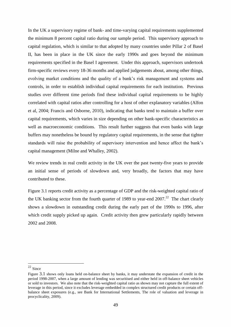
49
In the UK a supervisory regime of bank- and time-varying capital requirements supplemented
the minimum 8 percent capital ratio during our sample period. This supervisory approach to
capital regulation, which is similar to that adopted by many countries under Pillar 2 of Basel
II, has been in place in the UK since the early 1990s and goes beyond the minimum
requirements specified in the Basel I agreement. Under this approach, supervisors undertook
firm-specific reviews every 18-36 months and applied judgements about, among other things,
evolving market conditions and the quality of a bank‘s risk management and systems and
controls, in order to establish individual capital requirements for each institution. Previous
studies over different time periods find these individual capital requirements to be highly
correlated with capital ratios after controlling for a host of other explanatory variables (Alfon
et al, 2004; Francis and Osborne, 2010), indicating that banks tend to maintain a buffer over
capital requirements, which varies in size depending on other bank-specific characteristics as
well as macroeconomic conditions. This result further suggests that even banks with large
buffers may nonetheless be bound by regulatory capital requirements, in the sense that tighter
standards will raise the probability of supervisory intervention and hence affect the bank‘s
capital management (Milne and Whalley, 2002).
We review trends in real credit activity in the UK over the past twenty-five years to provide
an initial sense of periods of slowdown and, very broadly, the factors that may have
contributed to these.
Figure 3.1 reports credit activity as a percentage of GDP and the risk-weighted capital ratio of
the UK banking sector from the fourth quarter of 1989 to year-end 2007.22
The chart clearly
shows a slowdown in outstanding credit during the early part of the 1990s to 1996, after
which credit supply picked up again. Credit activity then grew particularly rapidly between
2002 and 2008.
22
Since
Figure 3.1 shows only loans held on-balance sheet by banks, it may understate the expansion of credit in the
period 1998-2007, when a large amount of lending was securitised and either held in off-balance sheet vehicles
or sold to investors. We also note that the risk-weighted capital ratio as shown may not capture the full extent of
leverage in this period, since it excludes leverage embedded in complex structured credit products or certain off-
balance sheet exposures (e.g., see Bank for International Settlements, The role of valuation and leverage in
procyclicality, 2009).
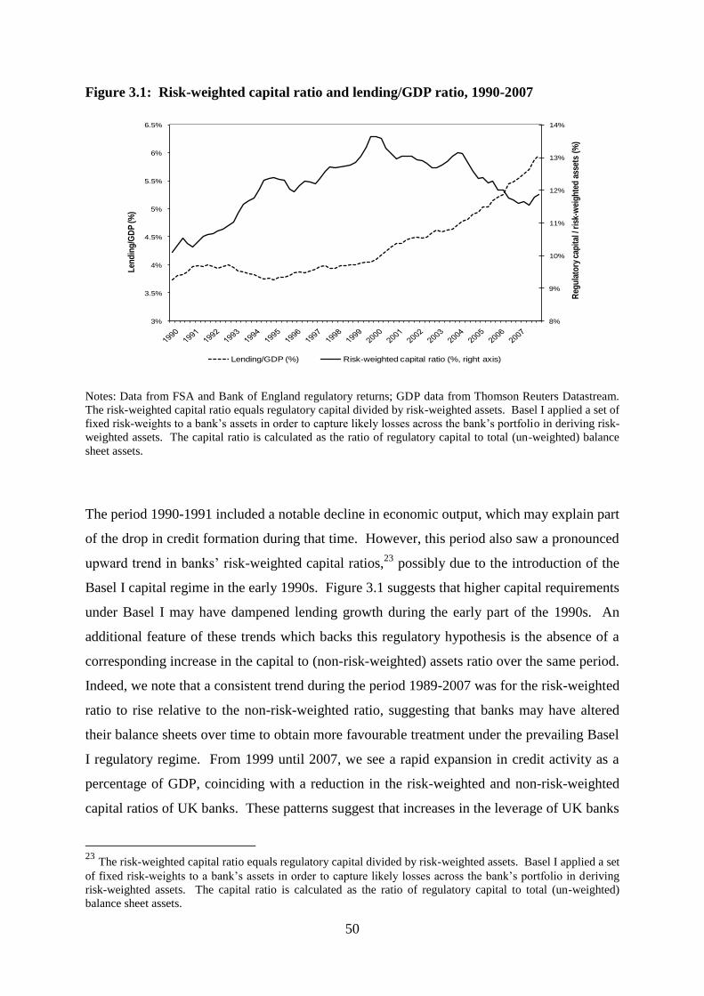
50
Figure 3.1: Risk-weighted capital ratio and lending/GDP ratio, 1990-2007
Notes: Data from FSA and Bank of England regulatory returns; GDP data from Thomson Reuters Datastream.
The risk-weighted capital ratio equals regulatory capital divided by risk-weighted assets. Basel I applied a set of
fixed risk-weights to a bank‘s assets in order to capture likely losses across the bank‘s portfolio in deriving risk-
weighted assets. The capital ratio is calculated as the ratio of regulatory capital to total (un-weighted) balance
sheet assets.
The period 1990-1991 included a notable decline in economic output, which may explain part
of the drop in credit formation during that time. However, this period also saw a pronounced
upward trend in banks‘ risk-weighted capital ratios,23
possibly due to the introduction of the
Basel I capital regime in the early 1990s. Figure 3.1 suggests that higher capital requirements
under Basel I may have dampened lending growth during the early part of the 1990s. An
additional feature of these trends which backs this regulatory hypothesis is the absence of a
corresponding increase in the capital to (non-risk-weighted) assets ratio over the same period.
Indeed, we note that a consistent trend during the period 1989-2007 was for the risk-weighted
ratio to rise relative to the non-risk-weighted ratio, suggesting that banks may have altered
their balance sheets over time to obtain more favourable treatment under the prevailing Basel
I regulatory regime. From 1999 until 2007, we see a rapid expansion in credit activity as a
percentage of GDP, coinciding with a reduction in the risk-weighted and non-risk-weighted
capital ratios of UK banks. These patterns suggest that increases in the leverage of UK banks
23
The risk-weighted capital ratio equals regulatory capital divided by risk-weighted assets. Basel I applied a set
of fixed risk-weights to a bank‘s assets in order to capture likely losses across the bank‘s portfolio in deriving
risk-weighted assets. The capital ratio is calculated as the ratio of regulatory capital to total (un-weighted)
balance sheet assets.
8%
9%
10%
11%
12%
13%
14%
3%
3.5%
4%
4.5%
5%
5.5%
6%
6.5%
Reg
ula
tory
cap
ital
/ ri
sk-w
eig
hte
d a
sset
s (%
)
Len
din
g/G
DP
(%)
Lending/GDP (%) Risk-weighted capital ratio (%, right axis)

51
sustained lending growth during this period. Indeed, global regulatory authorities cite a
credit boom fuelled by increased leverage as an important cause of the financial crisis that
began in 2007.24
While these aggregate series point to some reasons for changes in credit activity, it is difficult
to tell the extent to which capital requirements drove them based on aggregate data alone. It
is well known that bank lending decreases during periods of poor macroeconomic
performance, which, in turn, affects bank capital. This drop, however, stems at least partially
from a decline in investment activity or profitable lending opportunities and, thus, a
downward shift in the demand for credit in general during these periods. Of interest to our
research is to what extent banks' shifted their supply of loans during this time as a means of
dealing with increased regulatory pressure on capital adequacy.
The bank capital channel for the transmission of financial shocks into the real economy may
explain the contraction of credit supply during the early 1990s (and also during the distressed
period of 2008-09). Under the conditions that (i) banks do not have excess capital with
which to sustain credit supply following a shock to the capital position (e.g., a tightening of
capital regulation or monetary policy, or a decline in asset values), and (ii) there is an
imperfect market for bank equity such that raising new capital is costly for banks, the
financial structure of the bank affects the bank‘s supply of credit (e.g., see Van den Heuvel,
2004). Hence, a bank may find it optimal, following an increase in regulatory capital
standards, to reduce growth in higher risk-weighted assets, for example, by raising rates on
lending, requiring higher collateral, or rationing credit at existing rates. These responses may
lead to changes in macroeconomic outcomes if firms and consumers in the economy depend
on banks to obtain credit.
In addition to the UK‘s long-standing convention of imposing firm-specific capital
requirements, the nature of the UK banking sector makes it a good example for evaluating the
effects of capital regulation on bank behaviour. This benefit stems mainly from the fact that
the sector has a large domestic retail banking market dominated by UK-headquartered banks.
The sector also consists of a small number of large, domestic banks (for example, at year-end
2007, the top 10 banks held roughly 85% percent of assets in our sample), with assets
distributed relatively broadly across the UK rather than concentrated in local markets. It is
more likely, then, that domestic economic conditions affect all banks similarly via borrower
24
E.g., see FSA (2009), A Regulatory Response to the Banking Crisis, paragraph 3.6.
52
credit standards and demand for credit. This feature helps to isolate the impact of capital
regulation better and avoid the problem that can arise where correlation in capitalization and
local economic conditions is significant (for a widely cited example of a similar study of the
1990s credit crunch in the US, based on banks in New England, see Peek and Rosengren,
1995).
In addition, while our dataset (described in more detail below) includes all UK-owned banks
and our results are confined on the UK banking sector, they have implications that extend
beyond the UK given the considerable global reach of UK banks. Table 3.1 shows that just
prior to the start of the financial crisis, UK-owned banks had outstanding claims on foreign
counterparties amounting to over $4 trillion. This balance represents more than 14 percent of
all global foreign claims, illustrating the large international presence of UK banks and the
extent of UK banks‘ linkage with the global economy.25
Therefore, the effects of capital
requirements on the UK bank sector‘s lending and balance sheet management behaviour may
have direct and material impacts on the economies of other countries where borrowers are
dependent on UK banks (i.e., they cannot costlessly switch to alternative lenders).
Table 3.1: International claims of the UK financial services sector, 2007
Notes: Source is Bank for International Settlements.
25
See McGuire and Tarashev (2008) for further evidence on the large global role of UK banks.
Counterparty
location
Foreign claims
(US$mn)
% of total
UK claims
% of global
foreign claims
Europe 1,398,956 34.9% 5.0%
US 1,222,279 30.5% 4.3%
Asia 609,129 15.2% 2.2%
Latin America & Caribbean 221,374 5.5% 0.8%
Africa & Middle East 189,805 4.7% 0.7%
Other 363,448 9.1% 1.3%
Total 4,004,991 100.0% 14.2%
Memo: Global foreign claims 28,152,190
53
3.3 Framework for evaluating the impacts of capital requirements
In this section, we describe our approach to estimate the effects of regulatory capital
requirements on banks‘ adjustment of their balance sheets. Very briefly, our approach
involves three steps. First, we specify and estimate a partial adjustment model of bank
capital that depends on bank-specific features, including individual capital requirements
assigned by the UK‘s FSA. Second, we use the parameters from this model to derive each
bank‘s (unobservable) target capital and an index of a bank‘s capitalization (i.e., surplus or
deficit) relative to its target. Finally, we use this measure of bank capitalization to estimate
models of lending, balance sheet and capital growth.
3.3.1 The target capital ratio model
The first stage of our analysis is to establish the link between banks‘ choice of capital ratio
and regulatory capital requirements. Since banks can suffer regulatory penalties if they fall
below the capital requirement, it is not unreasonable to believe that where a bank operates
with a small buffer above the capital requirements, the long-run pass-through of changes in
the capital requirement into changes in the capital ratio will be substantial, perhaps even one-
for-one. However, we might also observe a significant pass-through for banks with large
capital buffers if banks hold buffers to guard against of regulatory breach and intervention
(see e.g., Furfine, 2001; Milne and Whalley, 2001). Supporting this idea, Figure 3.2 plots the
actual risk-weighted capital ratio against the bank and time-specific capital requirement for
our sample of UK banks). Although there is a large cluster of banks with relatively small
buffers of around 0-5 percentage points, many other banks have larger buffers. The figure
suggests a positive relationship between actual capital ratios and regulatory capital
requirements, and the banks with higher capital requirements also tend to hold higher buffers.

54
Figure 3.2: Risk-weighted capital ratios and supervisory capital requirements
Notes: Source is regulatory returns from the Bank of England and FSA. The bank- and time-specific capital
requirement are confidential and hence we group data within percentage point increments of the capital
requirement and show a box-and-whisker plot to show the distribution of capital ratios. As in standard box plots,
the boxes show the median and quartiles and whiskers show the adjacent values.
In order to verify the positive association between capital ratios and capital requirements after
controlling for other relevant factors, and to provide a specification of the target capital ratio
for the banks in our sample, we model each bank‘s target risk-weighted capital ratio (𝑘𝑖𝑡∗ ) as a
function of a vector of bank- and time-specific characteristics (𝑋𝑖𝑡 ), and a fixed effect (𝛼𝑖) for
each bank which captures idiosyncratic factors such as business model, management, risk
aversion and the mix of markets in which the bank operates. This specification takes the
following form:
𝑘𝑖𝑡∗ = 𝛼𝑖 + 𝜷′𝑿𝒊𝒕 (3.1)
We assume that banks take time to adjust their capital and assets towards their target capital
ratio, and we model this as a partial adjustment process following Hancock and Wilcox
(1994) and recently used in Berrospide and Edge (2010). This approach presumes, for a
number of practical and theoretical reasons, that capital adjustment costs preclude banks from
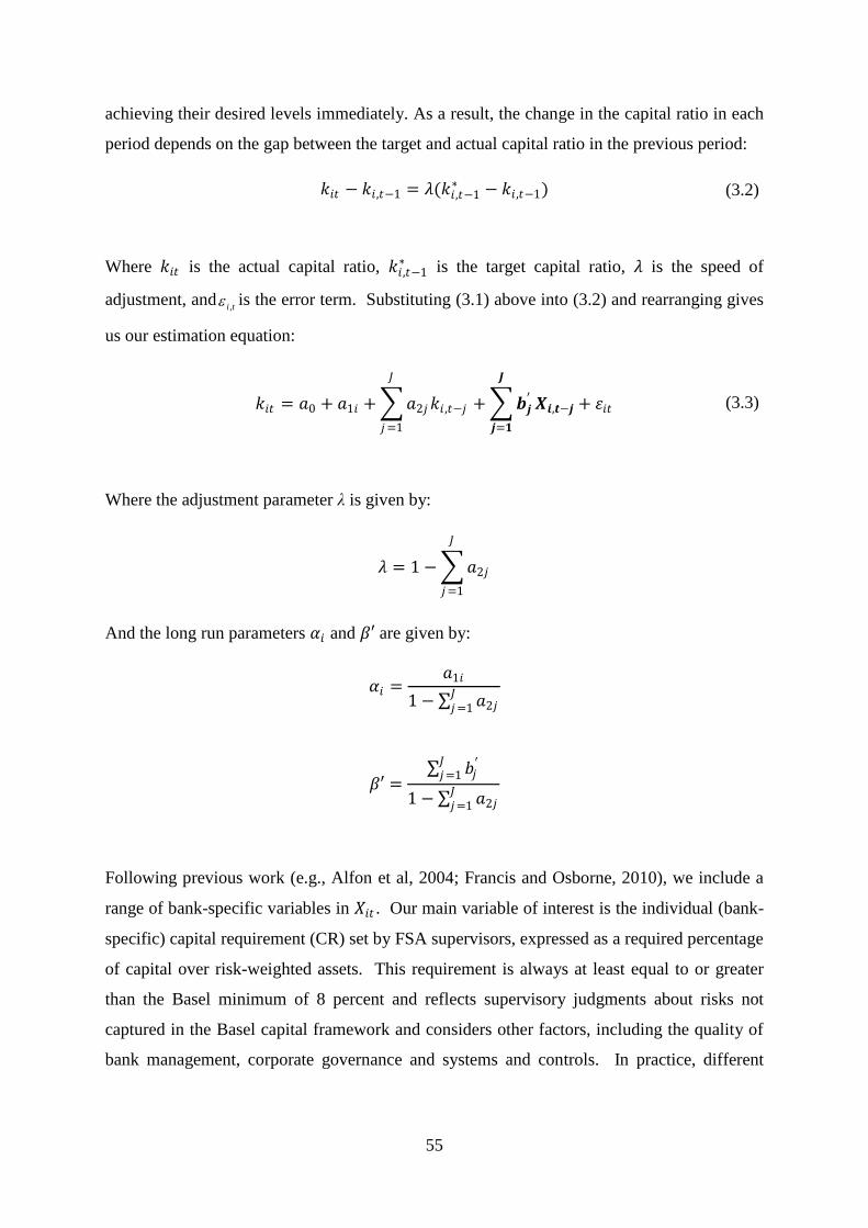
55
achieving their desired levels immediately. As a result, the change in the capital ratio in each
period depends on the gap between the target and actual capital ratio in the previous period:
𝑘𝑖𝑡 − 𝑘𝑖 ,𝑡−1 = 𝜆(𝑘𝑖 ,𝑡−1∗ − 𝑘𝑖 ,𝑡−1) (3.2)
Where 𝑘𝑖𝑡 is the actual capital ratio, 𝑘𝑖 ,𝑡−1∗ is the target capital ratio, 𝜆 is the speed of
adjustment, and is the error term. Substituting (3.1) above into (3.2) and rearranging gives
us our estimation equation:
𝑘𝑖𝑡 = 𝑎0 + 𝑎1𝑖 + 𝑎2𝑗𝑘𝑖 ,𝑡−𝑗
𝐽
𝑗=1
+ 𝒃𝒋′
𝑱
𝒋=𝟏
𝑿𝒊,𝒕−𝒋 + 휀𝑖𝑡 (3.3)
Where the adjustment parameter λ is given by:
𝜆 = 1 − 𝑎2𝑗
𝐽
𝑗=1
And the long run parameters 𝛼𝑖 and 𝛽′ are given by:
𝛼𝑖 =𝑎1𝑖
1 − 𝑎2𝑗𝐽𝑗=1
𝛽′ = 𝑏𝑗
′𝐽𝑗=1
1 − 𝑎2𝑗𝐽𝑗=1
Following previous work (e.g., Alfon et al, 2004; Francis and Osborne, 2010), we include a
range of bank-specific variables in 𝑋𝑖𝑡 . Our main variable of interest is the individual (bank-
specific) capital requirement (CR) set by FSA supervisors, expressed as a required percentage
of capital over risk-weighted assets. This requirement is always at least equal to or greater
than the Basel minimum of 8 percent and reflects supervisory judgments about risks not
captured in the Basel capital framework and considers other factors, including the quality of
bank management, corporate governance and systems and controls. In practice, different
ti,
56
capital requirements may apply to a bank‘s banking and trading books, so we use the overall
required ratio, calculated as a weighted average.
We include a number of other variables found useful in the literature on the determinants of
bank capital ratios to control for differences in banks‘ ability and incentives to adjust capital.
One likely determinant of a bank‘s desired capital ratio is the expected cost of failure, which
depends on the likelihood and cost of failure. The risk-weighted capital ratio already
includes a regulatory measure of risk embedded within it, but we include the ratio of risk-
weighted assets, as defined under Basel I, to total assets (RISK), to assess the relationship
between the risk-weighted capital ratio and the bank‘s risk profile. For example, a negative
association may indicate that riskier banks have lower risk-weighted capital ratios, which
could be consistent with moral hazard behaviour or a greater risk appetite. Since RISK is a
regulatory measure of portfolio risk, we also include the ratio of total provisions over on-
balance-sheet assets (PROVISIONS) as a proxy for banks‘ own internal estimates of risk.
This variable reflects management‘s assessment of the losses embedded in the bank‘s asset
portfolio. Since the composition of a bank‘s capital base may affect the capacity to absorb
losses, which may affect the market‘s perception of a bank‘s risk, we include the ratio of tier
1 over total capital (TIER1) as a proxy for the quality of capital. We also include a proxy for
bank size (SIZE), calculated as the time demeaned value of the log of total assets,26
as
previous studies argue that larger banks may be better able to diversify risks, access funding
and adjust capital compared with smaller institutions. To control for different business
models in banks with large trading books, we include the ratio of trading book assets to total
balance sheet assets (TB).27
Due to the presence of a lagged dependent variable, we estimate (3.3) using the system GMM
method for dynamic panels developed by Blundell and Bond (1998) and implemented in
Stata by Roodman (2009). We use the two-stage version with the Windmeijer correction to
the standard errors (Windmeijer, 2005).
26
We carry out time demeaning by calculating the mean log of total assets across all banks in each time period,
and then subtract this from each bank‘s log of total assets in each time period. We do this to avoid spurious
correlation between total assets and capital ratios resulting from non-stationarity of total assets. 27
The return on equity is often included in capital structure regressions (see section 2.1 and Chapter 5).
However, unfortunately it is unavailable in our sample since income statement data was not collected regularly
for much of our sample period.
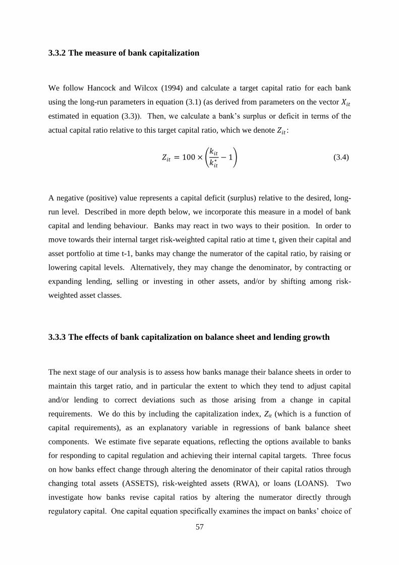
57
3.3.2 The measure of bank capitalization
We follow Hancock and Wilcox (1994) and calculate a target capital ratio for each bank
using the long-run parameters in equation (3.1) (as derived from parameters on the vector 𝑋𝑖𝑡
estimated in equation (3.3)). Then, we calculate a bank‘s surplus or deficit in terms of the
actual capital ratio relative to this target capital ratio, which we denote 𝑍𝑖𝑡 :
𝑍𝑖𝑡 = 100 ×
𝑘𝑖𝑡𝑘𝑖𝑡∗ − 1 (3.4)
A negative (positive) value represents a capital deficit (surplus) relative to the desired, long-
run level. Described in more depth below, we incorporate this measure in a model of bank
capital and lending behaviour. Banks may react in two ways to their position. In order to
move towards their internal target risk-weighted capital ratio at time t, given their capital and
asset portfolio at time t-1, banks may change the numerator of the capital ratio, by raising or
lowering capital levels. Alternatively, they may change the denominator, by contracting or
expanding lending, selling or investing in other assets, and/or by shifting among risk-
weighted asset classes.
3.3.3 The effects of bank capitalization on balance sheet and lending growth
The next stage of our analysis is to assess how banks manage their balance sheets in order to
maintain this target ratio, and in particular the extent to which they tend to adjust capital
and/or lending to correct deviations such as those arising from a change in capital
requirements. We do this by including the capitalization index, Zit (which is a function of
capital requirements), as an explanatory variable in regressions of bank balance sheet
components. We estimate five separate equations, reflecting the options available to banks
for responding to capital regulation and achieving their internal capital targets. Three focus
on how banks effect change through altering the denominator of their capital ratios through
changing total assets (ASSETS), risk-weighted assets (RWA), or loans (LOANS). Two
investigate how banks revise capital ratios by altering the numerator directly through
regulatory capital. One capital equation specifically examines the impact on banks‘ choice of

58
overall regulatory capital (REGK), while another looks more closely at the determinants of
higher-quality, tier 1 capital (TIER1).28
In each model, the dependent variable is the
quarterly growth rate, calculated as 100*(ln(xt)-ln(xt-1)), where x represents the balance sheet
element in question at time t.
Changes in the demand for loans, resulting from exogenous demand-side shocks or feedback
effects from developments in the financial sector, are likely contributors to fluctuations in
overall credit activity. For example, in the financial accelerator theory, (e.g., Bernanke,
Gertler and Gilchrist, 1999), shocks to the balance sheets of leveraged financial
intermediaries lead to asset sales and declining asset prices, reducing the credit-worthiness of
borrowers and hence the demand for loans. When shocks affect a large number of leveraged
financial intermediaries, the resulting adverse feedback loops may depress investment and
lead to a slow recovery (Brunnermeier and Sannikov, 2011). This theory suggests why in
2007 to 2008 borrower balance sheet effects may have played an important role in translating
relatively small mortgage losses into a full blown financial crisis (Brunnermeier, 2009).
Although we control for credit and macroeconomic conditions, it is beyond the scope of this
paper to examine second-round feedback effects of capital shocks via loan demand, and
hence our work is best viewed as a partial equilibrium analysis.
Whether changes in capital requirements produce feedback effects that further influence bank
behaviour and have significant second-round effects on economic activity depends on the
extent to which these changes impact banks in aggregate at once, especially if through the
credit channel. If banks respond to higher capital requirements by reducing the supply of
credit (e.g., by tightening lending standards or raising interest rates), then this response could
reduce the volume of productive investments that get funded, potentially lowering asset
prices and borrowers‘ net worth (and borrowing capacities) in turn. This effect can further
reduce economic activity and banks‘ net worth (and lending capacities), which again can feed
back on asset prices and so on. Indeed, dampening over-exuberant credit activity and
economic growth via this mechanism is an underlying objective of countercyclical capital
requirements under Basel III. As noted earlier, while we do not explicitly examine these
second-round effects, our paper provides a first step towards understanding how banks may
react to higher capital requirements.
28
Tier 1 capital consists mainly of core capital elements, including common stock, retained earnings and non-
cumulative preferred stock, all of which are readily available to absorb losses. Policymakers have recently
placed a lot more emphasis on requiring banks to hold much higher proportions of this type of capital in overall
regulatory capital.
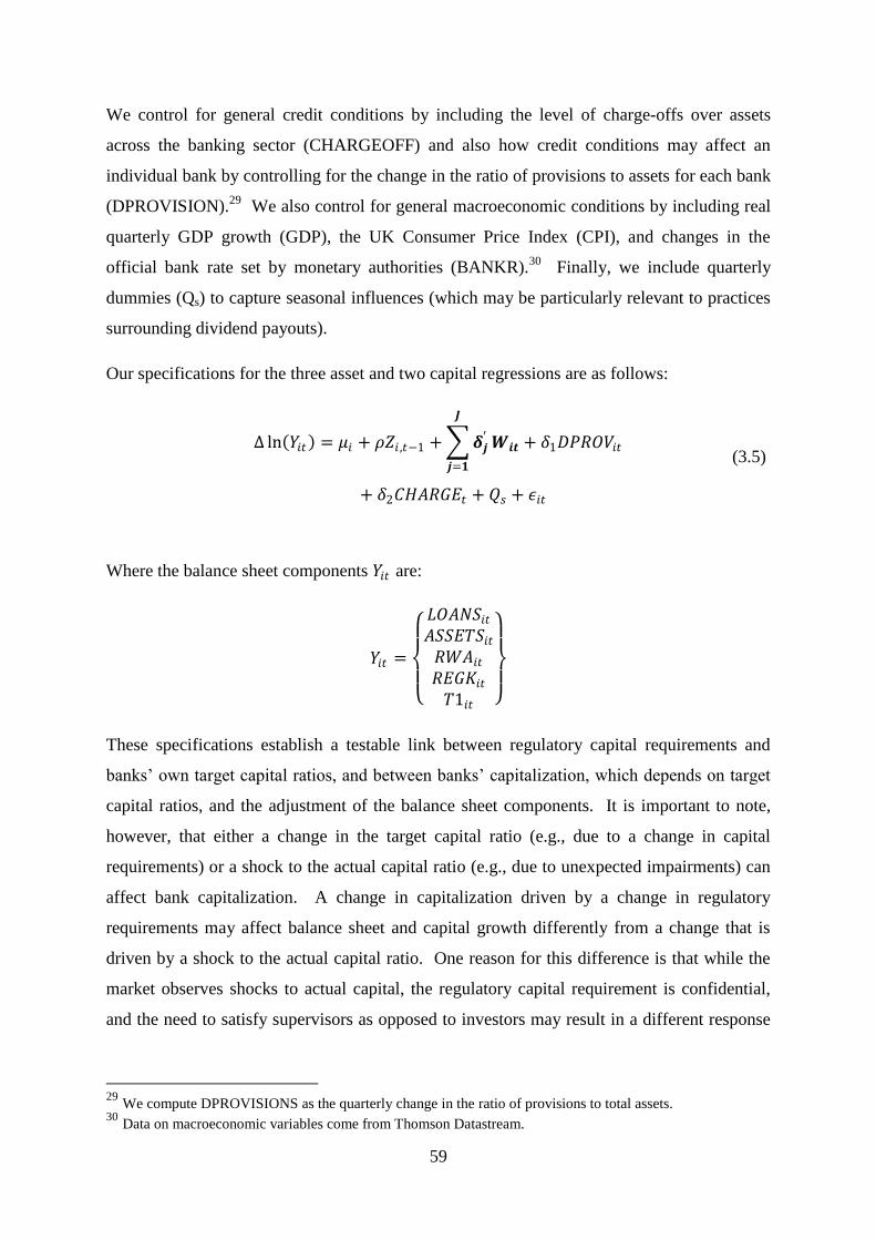
59
We control for general credit conditions by including the level of charge-offs over assets
across the banking sector (CHARGEOFF) and also how credit conditions may affect an
individual bank by controlling for the change in the ratio of provisions to assets for each bank
(DPROVISION).29
We also control for general macroeconomic conditions by including real
quarterly GDP growth (GDP), the UK Consumer Price Index (CPI), and changes in the
official bank rate set by monetary authorities (BANKR).30
Finally, we include quarterly
dummies (Qs) to capture seasonal influences (which may be particularly relevant to practices
surrounding dividend payouts).
Our specifications for the three asset and two capital regressions are as follows:
Δ ln 𝑌𝑖𝑡 = 𝜇𝑖 + 𝜌𝑍𝑖 ,𝑡−1 + 𝜹𝒋′
𝑱
𝒋=𝟏
𝑾𝒊𝒕 + 𝛿1𝐷𝑃𝑅𝑂𝑉𝑖𝑡
+ 𝛿2𝐶𝐻𝐴𝑅𝐺𝐸𝑡 + 𝑄𝑠 + 𝜖𝑖𝑡
(3.5)
Where the balance sheet components 𝑌𝑖𝑡 are:
𝑌𝑖𝑡 =
𝐿𝑂𝐴𝑁𝑆𝑖𝑡𝐴𝑆𝑆𝐸𝑇𝑆𝑖𝑡𝑅𝑊𝐴𝑖𝑡𝑅𝐸𝐺𝐾𝑖𝑡𝑇1𝑖𝑡
These specifications establish a testable link between regulatory capital requirements and
banks‘ own target capital ratios, and between banks‘ capitalization, which depends on target
capital ratios, and the adjustment of the balance sheet components. It is important to note,
however, that either a change in the target capital ratio (e.g., due to a change in capital
requirements) or a shock to the actual capital ratio (e.g., due to unexpected impairments) can
affect bank capitalization. A change in capitalization driven by a change in regulatory
requirements may affect balance sheet and capital growth differently from a change that is
driven by a shock to the actual capital ratio. One reason for this difference is that while the
market observes shocks to actual capital, the regulatory capital requirement is confidential,
and the need to satisfy supervisors as opposed to investors may result in a different response
29
We compute DPROVISIONS as the quarterly change in the ratio of provisions to total assets. 30
Data on macroeconomic variables come from Thomson Datastream.

60
from the firm. Therefore, accounting for these differences may be important when gauging
the possible impact of changes in regulatory capital requirements on banks‘ balance sheets.
To test how balance sheet adjustment differs in the face of a change in capital requirements,
we create a dummy variable (RECENT) which takes the value 1 whenever a known change
in capital requirements occurred in the last five quarters, and interact this with Zit to create a
new variable (𝑍𝑖 ,𝑡−1𝑅𝐸𝐶𝐸𝑁𝑇 ).
31 We then include this variable in our estimations of equation (3.5).
The amended specification is as follows:
Δ ln 𝑌𝑖𝑡 = 𝜇𝑖 + 𝜌1𝑍𝑖 ,𝑡−1 + 𝜌2𝑍𝑖 ,𝑡−1𝑅𝐸𝐶𝐸𝑁𝑇 + 𝜹𝒋
′
𝑱
𝒋=𝟏
𝑾𝒊𝒕
+ 𝛿1𝐷𝑃𝑅𝑂𝑉𝑖𝑡 + 𝛿2𝐶𝐻𝐴𝑅𝐺𝐸𝑖𝑡 + 𝑄𝑠 + 𝜖𝑖𝑡
(3.6)
The coefficient on the interaction term (𝜌2) represents the marginal impact of regulatory
capital requirements on balance sheet and capital growth, whereas 𝜌1 captures the effects of
deviations of capital from target more generally. Note that 𝜌1 also includes a regulatory
effect since banks that fall close to the regulatory minimum may face supervisory sanctions;
however, this is difficult to distinguish from the effects of market discipline32
, and this is the
motivation for our focus on changes in capital requirements. Testing whether 𝜌1 + 𝜌2 = 0
provides a more robust test of the hypothesis that capital requirements have an incremental
effect on banks‘ balance sheet management, though it is limited to occasions where capital
requirements have actually changed. The sum of the coefficients on 𝑍𝑖 ,𝑡−1 and on the
interaction term 𝑍𝑖 ,𝑡−1𝑅𝐸𝐶𝐸𝑁𝑇 (𝜌1 + 𝜌2) provides an overall measure of banks‘ balance sheet
adjustment to a change in bank capital requirements. We test the sum of these coefficients in
order to show whether the overall effect following a change in capital requirements is
statistically significantly different from zero.
These specifications allow for fixed effects across banks, as noted by the bank-specific
intercept, αi. It is also possible to model the balance sheet growth equations using a dynamic
specification, as in the target ratio equation above, by including lags of the dependent
variable. This approach is appropriate if partial adjustment more accurately describes banks‘
31
We don‘t know exactly when a change in capital requirements occurred, but we set the dummy equal to 1
when the capital requirement changes significantly from one quarter to the next. 32
In fact, as we noted earlier, a relationship similar to that captured by 𝜌1 - i.e. banks falling below target
capital ratios - has often been attributed to a regulatory effect in other studies.

61
balance sheet behaviour in the long run. To consider that possibility, we estimate equation
(3.6) with and without a lagged dependent variable (using fixed effects and system GMM
respectively). The results indicated that the coefficients on the lagged dependent variables
were not significantly different from zero, suggesting that banks fully adjust to their desired
level of long-run growth in each period. Hence, below we focus our discussion on results
from the static panel method, as specified in Equation (3.6).
3.4 Data and description of sample
Regulatory returns submitted to the FSA (and the Bank of England as legacy supervisor)
provide our main source of banking data. These returns are quarterly spanning 1996 to 2007
and include balance sheet information and confidential individual capital requirements on all
commercial banks authorised in the UK. We restrict our sample to unconsolidated reports
due to the UK practice of setting individual capital requirements at the level of the solo entity
as well as at the group (consolidated) level. This practice differs from that followed by many
other banking regulators that set capital requirements for the consolidated banking group only
(for further details, see Francis and Osborne, 2010). Since our objective is on isolating the
behaviour of individual banks in response to capital regulation, evaluating solo-level banking
data is important to this analysis. Data on macroeconomic control variables come from
Thompson Datastream and Bank of England sources.
We adjust the banking data for mergers and acquisitions by creating a new bank after such
events, identified using Dealogic data on mergers and acquisitions (M&A) activity by UK
banks. Since many structural changes in banks will not feature in this data (e.g., purchase or
sale of a major business line), we further adjust for these events, by creating a new bank
whenever both total assets and capital fall or rise by more than 30 percent.33
We make
further adjustments to the sample to account for extreme and missing values (which can cause
large variations in estimated parameters). In particular, to reduce the influence of missing or
outlier values, we first drop observations with zeros or missing values for total or risk-
weighted assets, the capital ratio, or capital requirements. We also drop banks with loan
growth, capital growth or asset growth greater than 50 percent or less than -50 percent, and
33
Such institutions represent approximately 1 percent of our sample.

62
banks with a capital ratio or capital requirement greater than 50 percent. This reduces our
sample size from 8566 to 5724. Although these cleaning exercises mean dropping a fair
number of observations, the extreme value observations tend to be from very small banks,
and the remaining banks account for over 90 percent of industry total assets on average,
showing that the final dataset remains representative of the UK financial sector during this
period.
Table 3.2 provides descriptive statistics on the variables used in our estimated equations.
Panel A reports information on the data used to estimate equation (3.3), our capital ratio
model. It shows that the average actual capital ratio for the entire sample is roughly 20
percent and significantly above the average capital requirement of 12 percent. The
significant gap is consistent with Figure 3.2 and the notion that banks generally hold sizeable
buffers to mitigate regulatory intervention. Capital requirements show considerably less
variation within banks than actual capital ratios, which likely reflect the less frequent
updating of this measure relative to actual ratios. Both actual and required capital ratios, and
indeed most of the variables intended to proxy banks‘ risk exposures and capital structure,
show more variation between than within banks, suggesting that we might expect differences
in capital ratios to reflect diversity in business models specific to banks rather than changes in
particular banks‘ circumstances over time.
Panel B shows summary statistics on our measure of the bank- and time-specific measure of
bank capitalization (Z) calculated using the coefficients in Table 3.3. These statistics show
that Z is, on average, slightly positive, suggesting that banks generally held excess capital
relative to their target capital ratio. The standard deviation is much higher within banks than
between banks. Figure 3.3 shows the distribution of bank capitalization over time and shows
that it varied considerably across banks at each point in time, with a gap of 10-20 percentage
points between the 25th
and 75th
percentile on average. It also shows that Z rose across the
banks in 2002-2003, before falling sharply across the distribution in 2004-2007, consistent
with a story of increasing leverage in this period.
Panel C of Table 3.2 reports descriptive statistics for the variables used in our balance sheet
growth models (Equation (3.6)). Quarter-on-quarter growth in each of these variables is
around 1.8 percent to 2.5 percent. Variation in each of these series is greater within banks
than between banks.
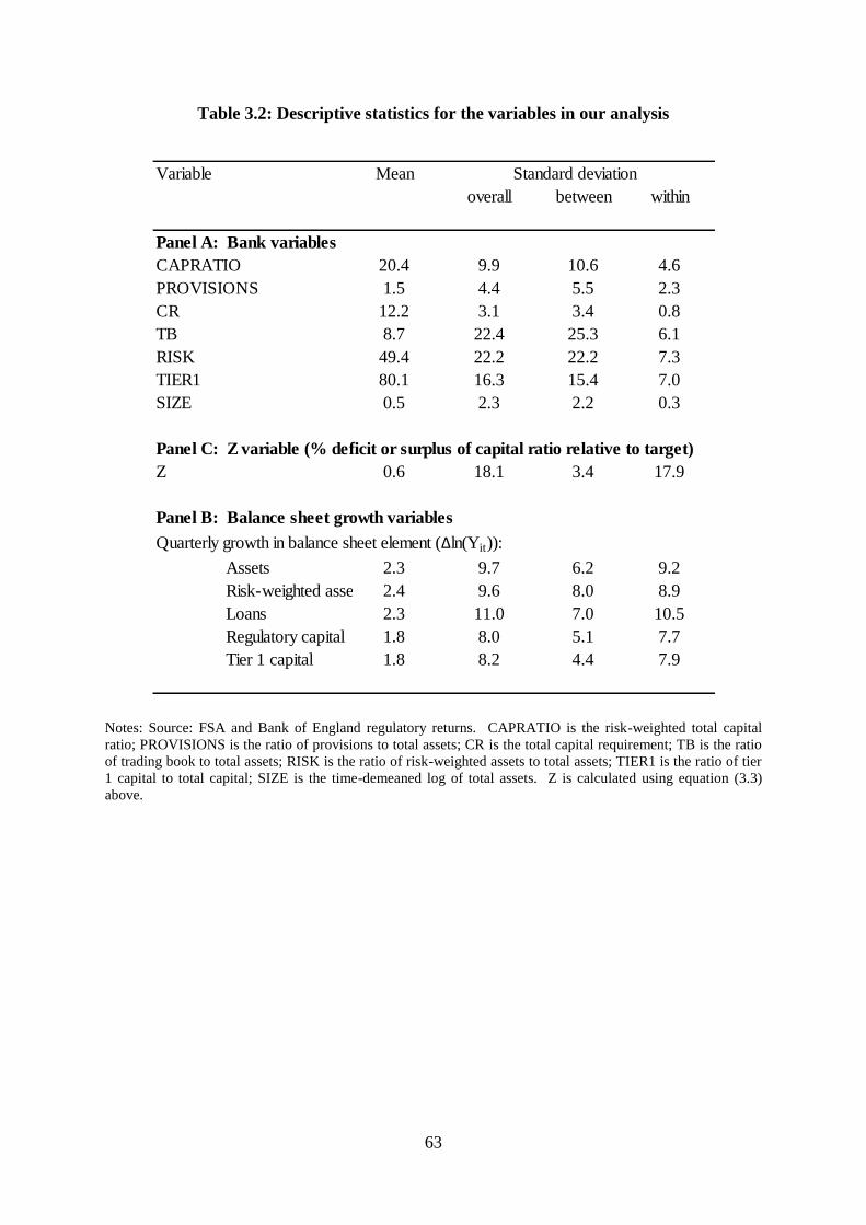
63
Table 3.2: Descriptive statistics for the variables in our analysis
Notes: Source: FSA and Bank of England regulatory returns. CAPRATIO is the risk-weighted total capital
ratio; PROVISIONS is the ratio of provisions to total assets; CR is the total capital requirement; TB is the ratio
of trading book to total assets; RISK is the ratio of risk-weighted assets to total assets; TIER1 is the ratio of tier
1 capital to total capital; SIZE is the time-demeaned log of total assets. Z is calculated using equation (3.3)
above.
Mean
overall between within
20.4 9.9 10.6 4.6
1.5 4.4 5.5 2.3
CR 12.2 3.1 3.4 0.8
TB 8.7 22.4 25.3 6.1
49.4 22.2 22.2 7.3
80.1 16.3 15.4 7.0
0.5 2.3 2.2 0.3
Panel C: Z variable (% deficit or surplus of capital ratio relative to target)
Z 0.6 18.1 3.4 17.9
Panel B: Balance sheet growth variables
Quarterly growth in balance sheet element (∆ln(Yit)):
Assets 2.3 9.7 6.2 9.2
Risk-weighted assets 2.4 9.6 8.0 8.9
Loans 2.3 11.0 7.0 10.5
Regulatory capital 1.8 8.0 5.1 7.7
Tier 1 capital 1.8 8.2 4.4 7.9
CAPRATIO
PROVISIONS
RISK
TIER1
SIZE
Variable Standard deviation
Panel A: Bank variables

64
Figure 3.3: Distribution of estimated Zit over time
Notes: Estimated using equation (3.3); see notes to Table 3.2.
3.5 Empirical results
3.5.1 Bank capital ratio
Table 3.3 presents the long-run coefficients from our final capital target model.34
Among our
set of bank-specific explanatory variables, the most important in determining capital ratios
over time are the individual capital requirement (CR) and the size of the bank (SIZE). The
results show a positive association between banks‘ capital ratios and individual capital
requirements, suggesting that banks react to higher (lower) requirements by raising
(reducing) their actual ratios. The results also indicate a negative relationship between capital
ratios and bank size, implying that larger banks tend to hold relatively lower capital ratios on
average. One possible explanation of this finding is that banks set their capital ratios
34 In preliminary regressions we also tested for a role of the ratio of subordinated debt to total capital, as a
measure of market discipline, and the return on equity, often used as a proxy for the cost of capital. Neither
variable proved statistically significant, so we omitted them from the final specification.
-20
-15
-10
-5
0
5
10
15
20
Zit (%
)
25th percentile 75th percentile Median
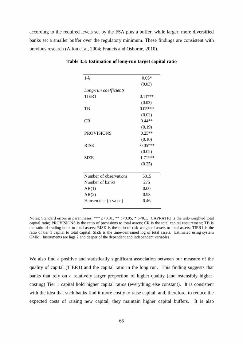
65
according to the required levels set by the FSA plus a buffer, while larger, more diversified
banks set a smaller buffer over the regulatory minimum. These findings are consistent with
previous research (Alfon et al, 2004; Francis and Osborne, 2010).
Table 3.3: Estimation of long-run target capital ratio
Notes: Standard errors in parentheses; *** p<0.01, ** p<0.05, * p<0.1. CAPRATIO is the risk-weighted total
capital ratio; PROVISIONS is the ratio of provisions to total assets; CR is the total capital requirement; TB is
the ratio of trading book to total assets; RISK is the ratio of risk-weighted assets to total assets; TIER1 is the
ratio of tier 1 capital to total capital; SIZE is the time-demeaned log of total assets. Estimated using system
GMM. Instruments are lags 2 and deeper of the dependent and independent variables.
We also find a positive and statistically significant association between our measure of the
quality of capital (TIER1) and the capital ratio in the long run. This finding suggests that
banks that rely on a relatively larger proportion of higher-quality (and ostensibly higher-
costing) Tier 1 capital hold higher capital ratios (everything else constant). It is consistent
with the idea that such banks find it more costly to raise capital, and, therefore, to reduce the
expected costs of raising new capital, they maintain higher capital buffers. It is also
1-λ 0.05*
(0.03)
Long-run coefficients
TIER1 0.11***
(0.03)
TB 0.05***
(0.02)
CR 0.44**
(0.19)
PROVISIONS 0.25**
(0.10)
RISK -0.05***
(0.02)
SIZE -1.71***
(0.25)
Number of observations 5815
Number of banks 275
AR(1) 0.00
AR(2) 0.93
Hansen test (p-value) 0.46

66
consistent with banks signalling balance sheet strength by maintaining both higher capital
ratios and a high proportion of high quality capital.
Table 3.3 also shows a significantly positive association between risk-based capital ratios and
our measure of bank trading activity (TB). The result indicates that, in the long run, targeted
capital ratios increase (decrease) as banks‘ involvement in trading activity increases
(decreases). We also find a negative relationship between our measure of regulatory risk in a
bank‘s portfolio (RISK) and the target capital ratio, suggesting that banks which are riskier
(as defined by Basel regulatory risk weights) may have better controls for mitigating this risk,
and hence hold lower capital against a given unit of risk-weighted assets. In contrast, we find
positive correlation between the bank‘s own view of portfolio risk (PROVISIONS) and the
target capital ratio, suggesting that target ratios are, on average, higher at banks as internal
views about expected losses increase.
The table also shows that while the adjustment parameter, calculated as the sum of the
coefficients on (two) lags of the dependent variable, is statistically significant at the 10
percent level, it is very small, suggesting that around 95 percent of the change in the long-run
target capital ratio is achieved within two quarters. At first sight, this finding suggests an
unrealistically fast adjustment process, especially given the costs associated with altering
either capital or risk-weighted assets. This result may be due, in part, to the UK regulatory
practice of informing banks of their individual capital requirements several months in
advance of the date on which they go into effect. This practice, as a result, provides banks
with some lead time in which to make adjustments prior to the date of the new capital
requirements.
3.5.2 Bank balance sheet adjustment
We report the results of our estimates of equation (3.6) in Table 3.4. The results show
significantly positive associations between our measure of bank capitalization (Zit) and each
of the three balance sheet elements of interest (total assets, risk-weighted assets, and loans).
The findings support the idea that lending and balance sheet growth is greater at banks with
excess capital (above desired targets). This finding is consistent with the idea that banks with
excess capital face less constraint on their ability to lend and/or grow compared with other
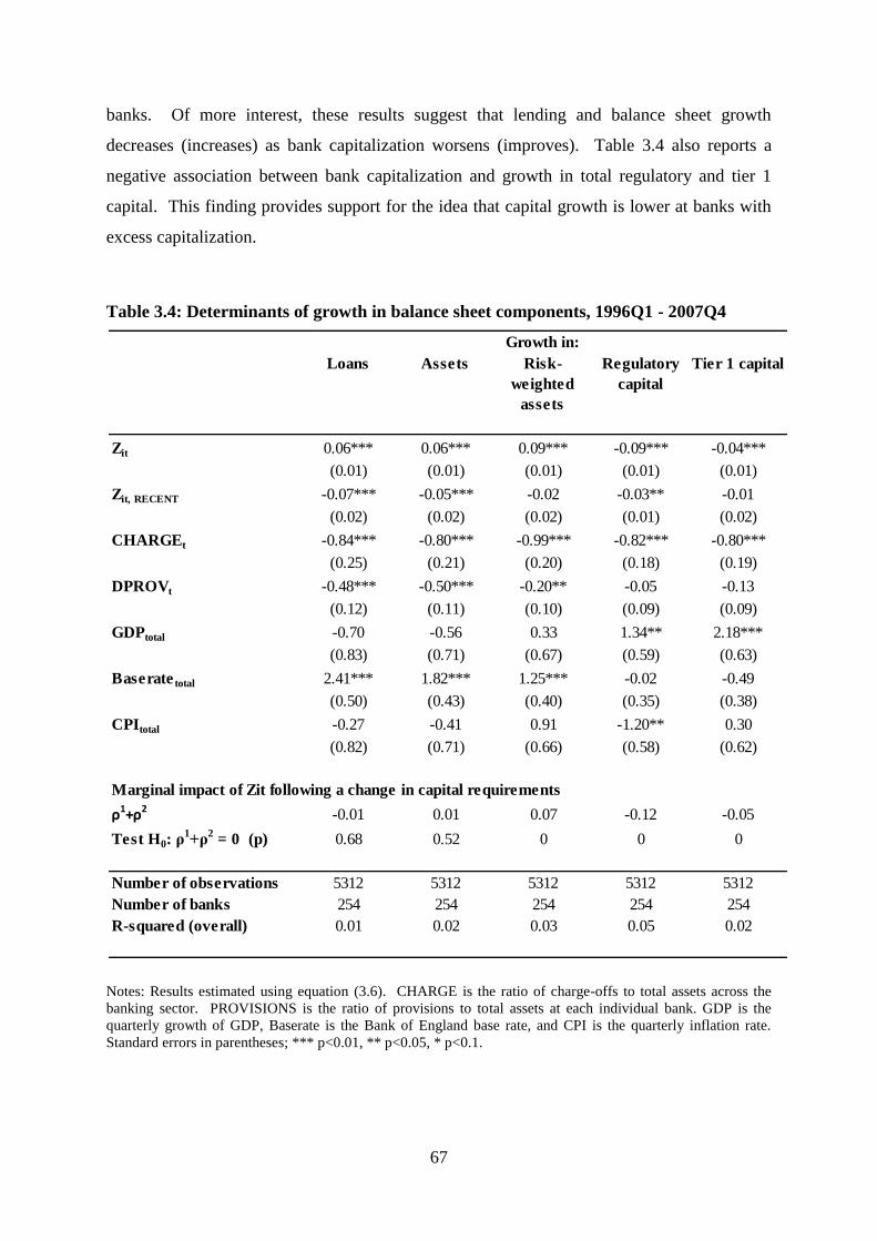
67
banks. Of more interest, these results suggest that lending and balance sheet growth
decreases (increases) as bank capitalization worsens (improves). Table 3.4 also reports a
negative association between bank capitalization and growth in total regulatory and tier 1
capital. This finding provides support for the idea that capital growth is lower at banks with
excess capitalization.
Table 3.4: Determinants of growth in balance sheet components, 1996Q1 - 2007Q4
Notes: Results estimated using equation (3.6). CHARGE is the ratio of charge-offs to total assets across the
banking sector. PROVISIONS is the ratio of provisions to total assets at each individual bank. GDP is the
quarterly growth of GDP, Baserate is the Bank of England base rate, and CPI is the quarterly inflation rate.
Standard errors in parentheses; *** p<0.01, ** p<0.05, * p<0.1.
Loans Assets Risk-
weighted
assets
Regulatory
capital
Tier 1 capital
Zit 0.06*** 0.06*** 0.09*** -0.09*** -0.04***
(0.01) (0.01) (0.01) (0.01) (0.01)
Zit, RECENT -0.07*** -0.05*** -0.02 -0.03** -0.01
(0.02) (0.02) (0.02) (0.01) (0.02)
CHARGEt -0.84*** -0.80*** -0.99*** -0.82*** -0.80***
(0.25) (0.21) (0.20) (0.18) (0.19)
DPROVt -0.48*** -0.50*** -0.20** -0.05 -0.13
(0.12) (0.11) (0.10) (0.09) (0.09)
GDPtotal -0.70 -0.56 0.33 1.34** 2.18***
(0.83) (0.71) (0.67) (0.59) (0.63)
Baserate total 2.41*** 1.82*** 1.25*** -0.02 -0.49
(0.50) (0.43) (0.40) (0.35) (0.38)
CPItotal -0.27 -0.41 0.91 -1.20** 0.30
(0.82) (0.71) (0.66) (0.58) (0.62)
Marginal impact of Zit following a change in capital requirements
ρ1+ρ2-0.01 0.01 0.07 -0.12 -0.05
Test H0: ρ1+ρ
2 = 0 (p) 0.68 0.52 0 0 0
Number of observations 5312 5312 5312 5312 5312
Number of banks 254 254 254 254 254
R-squared (overall) 0.01 0.02 0.03 0.05 0.02
Growth in:
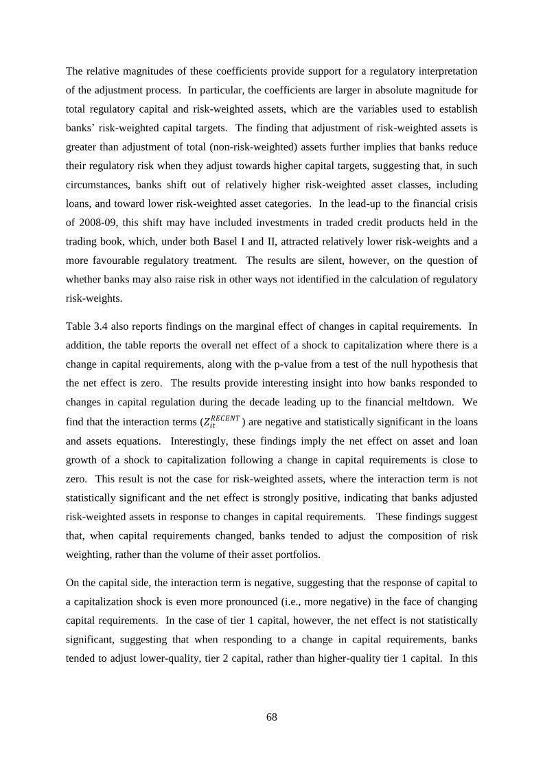
68
The relative magnitudes of these coefficients provide support for a regulatory interpretation
of the adjustment process. In particular, the coefficients are larger in absolute magnitude for
total regulatory capital and risk-weighted assets, which are the variables used to establish
banks‘ risk-weighted capital targets. The finding that adjustment of risk-weighted assets is
greater than adjustment of total (non-risk-weighted) assets further implies that banks reduce
their regulatory risk when they adjust towards higher capital targets, suggesting that, in such
circumstances, banks shift out of relatively higher risk-weighted asset classes, including
loans, and toward lower risk-weighted asset categories. In the lead-up to the financial crisis
of 2008-09, this shift may have included investments in traded credit products held in the
trading book, which, under both Basel I and II, attracted relatively lower risk-weights and a
more favourable regulatory treatment. The results are silent, however, on the question of
whether banks may also raise risk in other ways not identified in the calculation of regulatory
risk-weights.
Table 3.4 also reports findings on the marginal effect of changes in capital requirements. In
addition, the table reports the overall net effect of a shock to capitalization where there is a
change in capital requirements, along with the p-value from a test of the null hypothesis that
the net effect is zero. The results provide interesting insight into how banks responded to
changes in capital regulation during the decade leading up to the financial meltdown. We
find that the interaction terms (𝑍𝑖𝑡𝑅𝐸𝐶𝐸𝑁𝑇 ) are negative and statistically significant in the loans
and assets equations. Interestingly, these findings imply the net effect on asset and loan
growth of a shock to capitalization following a change in capital requirements is close to
zero. This result is not the case for risk-weighted assets, where the interaction term is not
statistically significant and the net effect is strongly positive, indicating that banks adjusted
risk-weighted assets in response to changes in capital requirements. These findings suggest
that, when capital requirements changed, banks tended to adjust the composition of risk
weighting, rather than the volume of their asset portfolios.
On the capital side, the interaction term is negative, suggesting that the response of capital to
a capitalization shock is even more pronounced (i.e., more negative) in the face of changing
capital requirements. In the case of tier 1 capital, however, the net effect is not statistically
significant, suggesting that when responding to a change in capital requirements, banks
tended to adjust lower-quality, tier 2 capital, rather than higher-quality tier 1 capital. In this
69
period, the option of changing tier 2 capital was relatively inexpensive,35
so these results are
consistent with the idea that banks choose the least costly way to respond to changes in
capital requirements.
Table 3.4 shows negative correlations between the growth in all of the balance sheet items
and the control variables accounting for credit conditions in each bank‘s portfolio,
DPROVISIONS and CHARGEOFFS. This result is consistent with the interpretation that
deterioration in the credit quality of borrowers (shown by higher losses, CHARGEOFFS, and
higher expected losses, DPROVISIONS) erodes banks‘ capital base and reduces credit
formation, as in the financial accelerator model described above.36
All of these coefficients
are statistically significant at the 10 percent level or better, with the exception of the
DPROVISIONS variable in the regressions of capital and tier 1 growth.
None of the controls for general macroeconomic conditions are consistently statistically
significant across all the five models. This result may be due, in part, to the fact that the
period of our analysis did not include substantial movements in economic conditions or
monetary policy. It is possible that banks may have been able to insulate their activities from
the relatively modest fluctuations in macroeconomic variables observed during this period.
Of the three macroeconomic variables, GDP is statistically significant in the two capital
growth models only. The absence of a significant association between lending growth and
GDP may be due to differences between banks in the extent to which customer demand for
bank credit varies over the cycle (e.g., see Huang, 2003). The positive and statistically
significant association between capital growth and GDP may reflect the relatively lower cost
of raising capital (through earnings and capital accretion) during more favourable economic
conditions.
The base rate set by the Bank of England is positive and statistically significant in all of the
asset growth specifications. At first sight, this result contrasts with expectations, since
increases in the base rate should pass through into consumer interest rates and hence suppress
demand for credit. One reason for this association may be that the policymakers setting
monetary policy may take into account bank credit when they are setting the level of base
35
Tier 2 capital is mostly made up of subordinated debt, which required only a small spread above the risk-free
rate during this period (see FSA consultation paper, Strengthening Capital Standards 2 (2006), Annex 2). 36
The impact on regulatory capital may stem from the treatment of bank loan loss provisions in regulatory
capital (i.e., they count towards regulatory capital up to a limit) and the effect that charge-offs have on loan
provisions (i.e., charge-offs reduce provisions and, therefore, regulatory capital).

70
rate, and hence strong credit growth may trigger increases in the base rate, which then take
time to act on demand for credit (e.g., because interest rates remain fixed for a time, or
consumers are unable to alter their reliance on bank borrowing in the short run). A second
explanation for this result is that while increases in interest rates may suppress demand for
credit, this change may actually result in firms becoming more dependent on banks, due to
the relatively high cost of securing credit from alternative sources during tight monetary
conditions (e.g., due to relationships between firms and banks that overcome information
asymmetries enhanced in periods of tight credit availability). For example, Huang (2003)
found that, for those large firms which account for the majority of borrowing from banks, the
relationship between monetary policy and credit growth is positive when fluctuations in
monetary policy are modest, but negative in periods of very tight monetary policy. Since the
period of our analysis falls into the former category,37
it is reassuring to know that our results
are consistent with this study. While the relationship between base rate and capital growth is
negative, which may reflect narrowing profit margins and declining asset valuations during
tight money periods, it is not statistically significant in either model.
Inflation is not an important determinant of bank balance sheet growth, since there is a
mixture of positive and negative coefficients on this variable, and it is only statistically
significant in one equation (growth in regulatory capital, where it is negative).
3.6 Policy implications
These results suggest how banks adjust their capital and assets in response to a change in
their capitalization (i.e., surplus or deficit capital relative to target) brought about by a change
in capital requirements. In this section, we quantify the effects of a countercyclical capital
requirement that increases regulatory minimums during a credit boom. We assume that the
UK regulator imposes three separate one percentage point (100 basis points) countercyclical
capital requirement add-ons in 1997, 2000 and 2003. We also assume that the UK banking
sector as a whole responds in the same way that we have estimated for individual banks.38
37
During our sample period, the base rate had a mean of 5.3 percent, a maximum value of 7.5 percent and a
standard deviation of just 1 percent. 38
These response rates allow us to estimate the effect of higher capital charges on balance sheet and capital
growth during the run-up to the financial crisis. Obviously, this ―what if‖ analysis is only an indicative, partial
71
The steps we take in the simulation are as follows:
1) Calculate new target capital ratio using the new capital requirements and the
parameters in Table 3, using aggregate banking industry data;
2) Calculate the Zit variable implied by the industry‘s actual capital ratio and the
new target capital ratio;
3) Take the actual historical growth in each balance sheet variable in each quarter
and adjust it by the Zit variable multiplied by the coefficients reported in Table 4;
and
4) Re-calculate the stocks of each balance sheet element in each period using the
adjusted growth schedule, allowing the resulting change in the capital ratio to feed
back onto the calculation of the Zit variable.
At the time of writing, the details of how exactly such a countercyclical capital requirement
might work in practice are still the subject of debate. Here we take a pragmatic approach and
assume that the UK authorities had identified an extended credit boom beginning in the late
1990s and ending in 2007, and, in response, implemented three separate increases in capital
requirements in 1997, 2000 and 2003 of one percentage point each time. These actions imply
that at the peak of the boom in 2007, capital requirements would be three percentage points
above their minimum level, which is consistent with initial proposals in the FSA‘s Turner
Review.
Table 3.5 reports the pro-forma impacts of the countercyclical capital requirements on each
balance sheet component, while Figure 3.4 shows the impact of the countercyclical capital
requirement on the growth in capital and risk-weighted assets over time. One can calculate
the response in two different ways; by using the base effect 𝜌1, which shows the effect of a
shock to capitalization, and using the net effect 𝜌1 + 𝜌2, which isolates the effect of a change
in capital requirements using a sub-sample of banks that experienced a change in their capital
requirements. While the latter is a more robust estimate of the incremental effect of capital
requirements, the former is a more general model of banks‘ responses to surplus or deficits of
capital estimated using much more data. It is worth noting that the former, more general
model, is still likely to include effects of capital requirements, and in fact is similar to the
equilibrium analysis, since it excludes possible feedback effects from the real economy back on to bank balance
sheets.

72
approach taken by most other studies by testing the response for banks falling close to (static)
capital requirements. Hence, the effect of changes in capital requirements is likely to be
between that predicted by the two versions of the model. Therefore, we show the impact
calculated using both approaches in Table 3.5, while Figure 3.4 only shows the impact using
the net effect.
In addition, we need to choose the adjustment of capital ratios to changes in capital
requirements. For example, our estimates indicate that the pass-through of a change in
capital requirements into the capital ratio would, on average, be around 40 percent, but given
a large enough increase, this implies that banks would end up with very low capital buffers,
raising the likelihood of a capital breach. Given the costs associated with breaching capital
requirements, larger increases in capital requirements are likely to lead to a much larger pass-
through, possibly approaching 100 percent, and therefore much more sizeable balance sheet
adjustments. As a result, in the second column of Table 3.5, we show the results of our
analysis assuming a 100 percent pass-through. In all cases the results are greater in
magnitude, and the increase in the capital ratio is equal to the full three percentage points
added to the capital requirement.
Consistent with the results presented in Table 3.4, when we use the net effect, the increase in
capital requirements has no effect on the absolute level of assets or loans, and so Figure 3.4
does not show the impact on these balance sheet elements. The stock of risk-weighted assets
falls to around 4 percent below the baseline by the end of the period. The absolute impact is
larger for regulatory capital, which increases to over 7 percent above the baseline.
Figure 3.4 shows that the policy helps to ensure that at the peak of a boom, banks have capital
ratios which provide a buffer against loan and other losses in the ensuing downturn. The
speeds of adjustment implied by our parameter estimates mean that by the end of 2007, the
banking sector capital ratio is 1.3 percentage points above the baseline capital ratio.
However, only about half of this increase in capital is high quality capital since the risk-
weighted tier 1 capital ratio only rises by 0.6 percentage points. This means that the resulting
buffer may have had a limited impact on banks‘ capacity to absorb losses as a going concern.

73
Table 3.5: Simulation of effects of 3 percentage point increase in capital requirements
44% (based on Table 3) 100%
Assets -3.40% -7.10%
Loans -3.40% -7.10%
-5.10% -10.60%
Total
capital 5.40% 11.80%
2.30% 5.10%
1.30% 3.00%
0.60% 1.30%
44% (based on Table 3) 100%
Assets 0.00% 0.00%
Loans 0.00% 0.00%
-4.40% -9.20%
Total
capital 6.20% 13.70%
2.00% 4.40%
1.30% 3.00%
0.50% 1.10%
Difference from baseline of:
Using coefficients on Z it (showing effect of shocks to capitalization)
Pass-through of capital requirements to target
capital ratio
Difference from baseline of:
Risk-weighted assets
Tier 1 capital
Increase in (percentage points):
Total capital ratio
Tier 1 capital ratio
Using net effects of a change in capital requirements, Z it +Z itRECENT (based on small sub-
sample of banks with recent changes to capital requirements)*
Pass-through of capital requirements to target
capital ratio
Risk-weighted assets
Tier 1 capital
Increase in (percentage points):
Total capital ratio
Tier 1 capital ratio
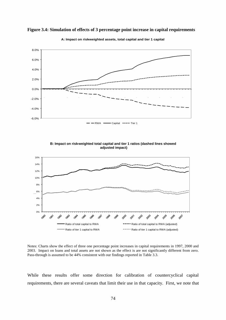
74
Figure 3.4: Simulation of effects of 3 percentage point increase in capital requirements
Notes: Charts show the effect of three one percentage point increases in capital requirements in 1997, 2000 and
2003. Impact on loans and total assets are not shown as the effect is are not significantly different from zero.
Pass-through is assumed to be 44% consistent with our findings reported in Table 3.3.
While these results offer some direction for calibration of countercyclical capital
requirements, there are several caveats that limit their use in that capacity. First, we note that
- 6.0%
- 4.0%
- 2.0%
0.0%
2.0%
4.0%
6.0%
8.0%
1995
1997 1998 1999 2000 2001 2002 2003 2004 2005 2006 2007
A: Impact on risk - weighted assets, total capital and tier 1 capital
RWA Capital Tier 1
0%
2%
4%
6%
8%
10%
12%
14%
16%
Capital ratio (%)
B: Impact on risk - weighted total capital and tier 1 ratios (dashed lines showed adjusted impact)
Ratio of total capital to RWA Ratio of total capital to RWA (adjusted)
Ratio of tier 1 capital to RWA Ratio of tier 1 capital to RWA (adjusted)

75
our estimates reflect a UK capital regime that, in general, imposed relatively small add-ons at
irregular intervals to individual banks. The impact of a large increase that is coordinated
across banks may be very different. For example, such an increase would be visible to the
market which would increase the extent of pass-through.
Second, our results do not capture possible feedback effects from the real economy back onto
bank balance sheets resulting from an increase in capital requirements. Our results reflect the
potential impact of modest idiosyncratic shocks to individual banks‘ capital adequacy only.
A coordinated and more substantial increase in capital requirements across major banks
would likely have knock-on effects on the demand for credit as firms and households become
less credit-worthy and asset prices rise more slowly than under a less systematic and stringent
scenario. These feedback effects could magnify the influence of the policy change.
The third issue is that our results reflect bank behaviour under the Basel I capital regime,
which is notably different from the Basel II standards and the revisions recently set out under
Basel III. Under the new regimes, capital requirements depend much more on banks‘ internal
models and credit ratings, in turn, affected by economic conditions.39
As a result, banks‘
capital management practices, and, in particular, the influence of regulatory capital
requirements, which were shown to play a key role in our results above, may have a different
influence under the new Basel framework. One consequence of the use of internal models
and credit ratings in Basel II is that it could result in capital requirements that amplify the
cycle, falling in good times and then rising in bad times.40
This procyclical effect was not
evident under the old Basel I regime and, therefore, during our estimation period, our analysis
of an assumed countercyclical capital policy would also need to consider a concomitant
decline in capital requirements on banks‘ asset portfolios (e.g., due to better internal ratings
and lower risk weights that arise during more favourable conditions).41
Calibrating
countercyclical capital requirements in a world of risk-sensitive capital requirements will,
undoubtedly, require further research.
39
Basel II introduced ratings-based and internal models based risk weights for credit risk, which accounts for
the majority of risk-weighted assets in UK banks. Although the measures in Basel III increase risk weights in
some ways (e.g. increasing market risk capital requirements and introducing a leverage ratio), they exclude
substantial changes to the use of internal models for credit risk. 40
There is an extensive literature on this issue, also known as procyclicality. See, for example, Altman and
Saunders, 2001; Gordy and Howells, 2006; Repullo et al, 2010. Assessments of the scale of the procyclicality
effects are difficult given the financial crisis which coincided with the introduction of Basel II in many
countries. 41
For example, a proposal to address this issue by varying the calibration of capital requirements over the cycle
has been made by Repullo and Suarez on the VoxEU website, July 2008, ―The procyclical effects of Basel II‖.
76
Finally, the Basel III agreement included a much tighter definition of capital and increases
the requirements for tier 1 capital and core tier 1 capital. As discussed above, to the extent
that capital raising cost considerations explain our balance sheet adjustment estimates above,
then the more stringent mandates about capital quality may further affect bank behaviour.
With a tighter definition of capital, which will require firms to raise common equity or retain
profits to increase their capital base, the greater cost of raising these higher quality forms of
capital compared to the debt-like, tier-2 capital may shift more of the burden of adjustment
onto loans and other assets. Hence, it is not unreasonable to believe that the impact of a
given change in capital requirements on loans and risk-weighted assets may be greater under
the Basel III regime.
3.7 Extension to the crisis period
The results presented above are from the period 1996-2007, which, in retrospect, was a
unique period of benign market conditions and sustained growth and profitability for the UK
banking system. Those results are useful in that they show what the effects of changes to
capital requirements are under such conditions, and we have used the results to simulate the
effects of a counter-cyclical increase in capital requirements. However, it is also important to
ask to what extent the results apply in the crisis period. The motivations are two-fold. First,
in the Basel III Accord, global regulators have agreed to move towards substantially higher
capital requirements, and choosing the calibration of these capital requirements and the speed
of their introduction requires evidence about the effects of capital requirements on bank
behaviour under stressed market conditions. Second, counter-cyclical capital requirements as
envisaged by Basel III are intended to fall during stressed market conditions in order to
stimulate new credit growth, and so evidence of bank reactions during the crisis is valuable.
Carrying out a similar analysis as above using data from the crisis period poses three
significant problems. First, while bank- and time-specific supervisory capital add-ons
continued to be imposed after 2007, in the crisis period these took a lesser role as the FSA
reacted to unfolding events and imposed higher capital requirements at a tier 1 capital level.
First, in late 2007 supervisors began to require large banks to hold core capital of at least 5%,
and then in 2008 a set of standards was introduced which required 8% tier 1 capital and 6%
core tier 1 capital. In 2010 the new Basel III standards were announced, and although they
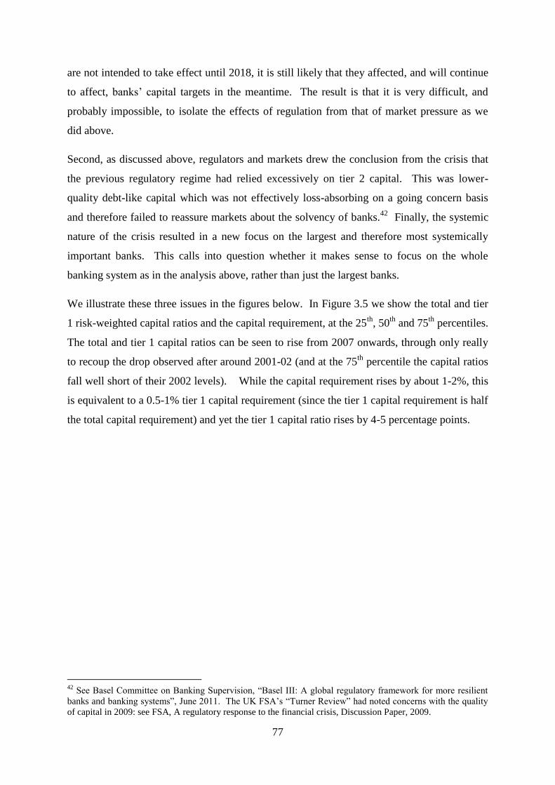
77
are not intended to take effect until 2018, it is still likely that they affected, and will continue
to affect, banks‘ capital targets in the meantime. The result is that it is very difficult, and
probably impossible, to isolate the effects of regulation from that of market pressure as we
did above.
Second, as discussed above, regulators and markets drew the conclusion from the crisis that
the previous regulatory regime had relied excessively on tier 2 capital. This was lower-
quality debt-like capital which was not effectively loss-absorbing on a going concern basis
and therefore failed to reassure markets about the solvency of banks.42
Finally, the systemic
nature of the crisis resulted in a new focus on the largest and therefore most systemically
important banks. This calls into question whether it makes sense to focus on the whole
banking system as in the analysis above, rather than just the largest banks.
We illustrate these three issues in the figures below. In Figure 3.5 we show the total and tier
1 risk-weighted capital ratios and the capital requirement, at the 25th
, 50th
and 75th
percentiles.
The total and tier 1 capital ratios can be seen to rise from 2007 onwards, through only really
to recoup the drop observed after around 2001-02 (and at the 75th
percentile the capital ratios
fall well short of their 2002 levels). While the capital requirement rises by about 1-2%, this
is equivalent to a 0.5-1% tier 1 capital requirement (since the tier 1 capital requirement is half
the total capital requirement) and yet the tier 1 capital ratio rises by 4-5 percentage points.
42
See Basel Committee on Banking Supervision, ―Basel III: A global regulatory framework for more resilient
banks and banking systems‖, June 2011. The UK FSA‘s ―Turner Review‖ had noted concerns with the quality
of capital in 2009: see FSA, A regulatory response to the financial crisis, Discussion Paper, 2009.

78
Figure 3.5: Tier 1 capital ratio for all banks, 1989Q4-2011Q2
Notes: Chart shows the total and tier 1 (risk-weighted) capital ratios and the supervisory capital requirement at
the 25th
, 50th
and 75th
percentiles in each quarter from 1984Q1 to 2011Q2. Source: Bank of England and FSA
regulatory returns.
0
10
20
30
40
50
60
Total capital ratio (%)
p25 p50 p75
0
10
20
30
40
50
60
Tier 1 capital ratio (%)
p25 p50 p75
8
9
10
11
12
13
14
15
16
17
Capital requirement (%)
p25 p50 p75
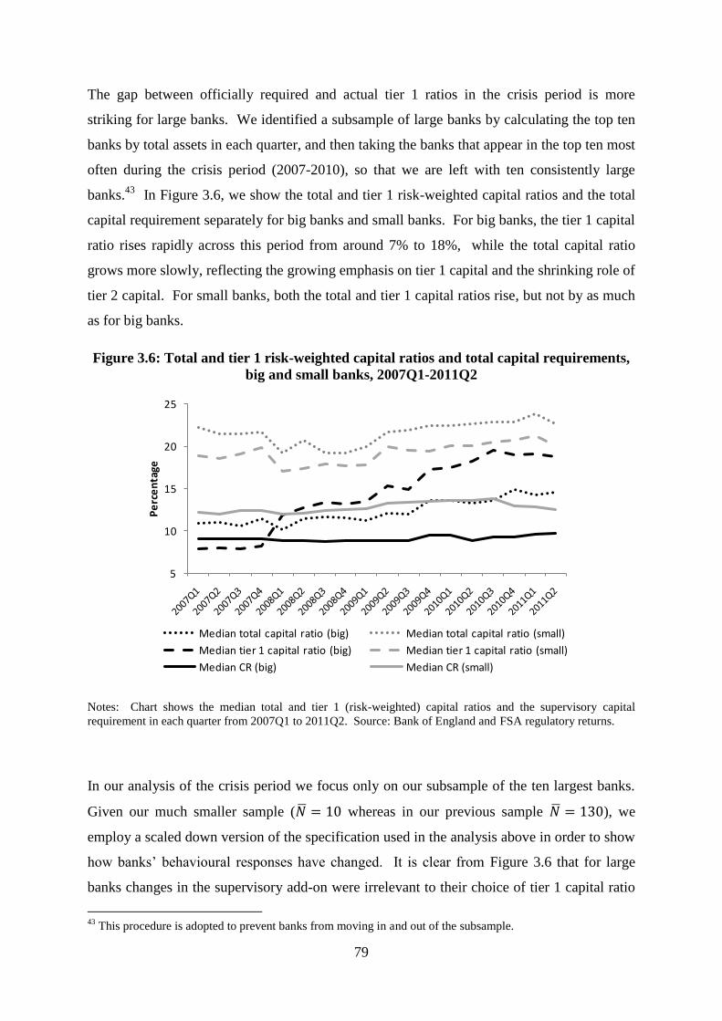
79
The gap between officially required and actual tier 1 ratios in the crisis period is more
striking for large banks. We identified a subsample of large banks by calculating the top ten
banks by total assets in each quarter, and then taking the banks that appear in the top ten most
often during the crisis period (2007-2010), so that we are left with ten consistently large
banks.43
In Figure 3.6, we show the total and tier 1 risk-weighted capital ratios and the total
capital requirement separately for big banks and small banks. For big banks, the tier 1 capital
ratio rises rapidly across this period from around 7% to 18%, while the total capital ratio
grows more slowly, reflecting the growing emphasis on tier 1 capital and the shrinking role of
tier 2 capital. For small banks, both the total and tier 1 capital ratios rise, but not by as much
as for big banks.
Figure 3.6: Total and tier 1 risk-weighted capital ratios and total capital requirements,
big and small banks, 2007Q1-2011Q2
Notes: Chart shows the median total and tier 1 (risk-weighted) capital ratios and the supervisory capital
requirement in each quarter from 2007Q1 to 2011Q2. Source: Bank of England and FSA regulatory returns.
In our analysis of the crisis period we focus only on our subsample of the ten largest banks.
Given our much smaller sample (𝑁 = 10 whereas in our previous sample 𝑁 = 130), we
employ a scaled down version of the specification used in the analysis above in order to show
how banks‘ behavioural responses have changed. It is clear from Figure 3.6 that for large
banks changes in the supervisory add-on were irrelevant to their choice of tier 1 capital ratio
43
This procedure is adopted to prevent banks from moving in and out of the subsample.
5
10
15
20
25
Pe
rce
nta
ge
Median total capital ratio (big) Median total capital ratio (small)
Median tier 1 capital ratio (big) Median tier 1 capital ratio (small)
Median CR (big) Median CR (small)
80
in this period, since while the add-ons did not vary over the period 2007-2010, the tier 1
capital ratio rose substantially, and well above the required levels (half of the total required
ratio or around 4.5% for the big banks). Instead, banks appear to have responded to sector-
wide regulatory and market pressure to raise capital tier 1 ratios. Without bank- and time-
varying capital ratios, it is difficult to identify the banks‘ target capital ratios as a function of
capital requirements over this period. Therefore we instead use a model of target capital
ratios in which banks‘ target capital ratios 𝑘𝑖𝑡∗ are expressed as a function of RISK, SIZE, TB
and TIER1.44
We also allow for bank effects, to control for unobserved differences in
business model or risk appetite as above, and time effects to control for time-specific
macroeconomic shocks and market and regulatory targets.
𝑘𝑖𝑡∗ = 𝛼𝑖
1 + 𝜃𝑡1 + 𝛽′𝑋𝑖𝑡 (3.7)
The deviation of capital from target is given by (𝐷𝐸𝑉𝑖𝑡 = 𝑘𝑖𝑡 − 𝑘𝑖𝑡∗ ) and this model can be
nested inside a model of the growth of balance sheet elements similar to (3.7) above:
Δ𝑙𝑛𝑌𝑖𝑡 = 𝛼𝑖2 + 𝜃𝑡
2+ 𝜌𝐷𝐸𝑉𝑖 ,𝑡−1 + 𝛿′𝑋𝑖𝑡 + 휀𝑖𝑡
= 𝛼𝑖2 + 𝜃𝑡
2 + 𝜌𝑘𝑖𝑡 + Π′𝑋𝑖𝑡 + 휀𝑖𝑡 (3.8)
where 𝜌 is the effect of deviations of tier 1 capital ratio from the target, and Π′ = 𝜌𝛽′ + 𝛿′ is
the composite effects of the explanatory variables on 𝑘𝑖𝑡∗ and Δ𝑙𝑛𝑌𝑖𝑡 . The advantage of this
more parsimonious specification is that one-stage estimation is more efficient, which is
appropriate for our small sample. However, it does not allow us to decompose the effects of
explanatory variables 𝑋𝑖𝑡 on the target capital ratio and the balance sheet components.45
Equation (3.8) is estimated separately for each of the Δ𝑙𝑛𝑌𝑖𝑡 (RWA, total assets, total capital
44
In the model above we also included PROVISIONS, but reporting changes mean that this is no longer
available on a consistent basis. Due to the implementation of Basel II from 2007, the RISK variable may not be
fully consistent with the pre-2007 period since it will be tied more closely to banks‘ own estimates of risk
weights. 45
A further disadvantage is that it does not allow us to adjust for the dynamics of adjustment to target capital.
However, achieving this is in any case made difficult by the fact that our cross-section sample is too small for us
to use the system GMM method to adjust for lagged dependent variable bias as above. The corrected LSDV
estimator by Bruno (2005) is an option but unfortunately does not allow more than one lag of the dependent
variable, making our original specification impossible to estimate.

81
and tier 1 capital)46
in the pre-crisis period (1996Q1-2006Q4) and the crisis period (2007Q1-
2011Q2).
In Table 3.6 below we show summary statistics for each of the variables included in (8),
separately for 1996Q1-2006Q4 and 2007Q1-2011Q2. The growth in risk-weighted assets is
much smaller in the later period, which may indicate the slowing supply of credit and other
services to the real economy during the crisis. Asset growth is however very similar across
the two periods, so the contraction may have been focused on relatively high risk-weighted
asset categories, a finding which is supported by a decline in the average risk weighting,
RISK.47
Tier 1 capital grows at a similar rate across the two periods, but total capital grows
more slowly in the crisis period, which reflects the growing emphasis on tier 1 capital.
Indeed, the share of tier 1 capital in total capital (TIER 1) is much higher in the second
period.
Table 3.6: Summary statistics for variables in analysis, big banks only
Notes: TIER 1 RATIO is the risk-weighted tier 1 capital ratio; TB is the ratio of trading book to total assets;
RISK is the ratio of risk-weighted assets to total assets; TIER1 is the ratio of tier 1 capital to total capital; SIZE
is the time-demeaned log of total assets. Estimated using two-way (bank and time) fixed effects.
46
It was not possible to include growth in loans since this is not available on a consistent basis across the two
periods. 47
It is difficult to say in retrospect which these would have been since under Basel II banks calculate their own
risk weights. Indeed, a bank may have altered the calculation methodology itself to improve capital ratios (see
e.g. see ―Fears rise over banks‘ capital tinkering‖, Financial Times, November 2011, and as a consequence it is
difficult to tell to what extent the trend reflects a genuine retreat from risk.
Mean Standard
deviation
(overall)
Mean Standard
deviation
(overall)
Growth in:
risk-weighted assets 2.6 7.0 1.0 11.1
asset growth 3.1 8.5 3.2 10.9
total capital 3.2 17.1 2.4 11.5
tier 1 capital 0.1 0.9 0.1 0.2
TIER 1 RATIO 7.4 2.2 13.7 6.1
TB 15.1 24.0 19.1 18.6
RISK 51.8 14.2 37.1 16.4
TIER1 64.7 14.7 107.3 45.6
SIZE 18.0 1.0 19.5 0.8
1996-2006 2007-2011

82
Next, in Table 3.7 we show the results of estimating equation (8) for each of the balance
sheet components Δ𝑙𝑛𝑌𝑖𝑡 . The tier 1 capital ratio has the expected sign for all equations i.e.
positive for asset variables and negative for capital variables. According to these results, in
the pre-crisis period (1996-2006), un-weighted assets and total capital were the main ways for
banks to adjust their capital ratios. Tier 1 capital was also significant, but the coefficient is
much lower in magnitude than total capital, suggesting that banks preferred to adjust their tier
2 capital rather than tier 1 capital. In the crisis period, the effect of tier 1 capital ratio on risk-
weighted assets is greater in magnitude than in the pre-crisis period and highly significant,
whereas asset growth is no longer significant, suggesting that risk adjustments became a more
common way for banks to adjust their capital ratios in the crisis period. Banks have been
actively seeking ways to reduce their risk-weighted assets over the crisis period, including by
selling portfolios of risky assets. Total capital is still highly significant but with a much
reduced coefficient, although the tier 1 capital ratio is similarly smaller in magnitude during
the crisis. Overall the results suggest that adjustments in portfolio risk, whether through asset
composition or changes in risk weights, were the most important method for banks to adjust
their capital ratios in the crisis period, and capital adjustments declined in importance. This
may reflect the increased cost of raising capital under stressed market conditions, and low
profitability providing limited funds to rebuild the capital base. A large part of the new
capital banks had by 2011 was a result of the equity injections made by the government in
late 2008, a large one-off injection which may not be captured well in our model.
Among the other coefficients, a higher share of assets in the trading book (TB) is negatively
associated with growth in RWA in both periods, and negatively associated with growth in
total and tier 1 capital, though the latter findings are not significant in the crisis period. This
may reflect the relatively low risk weighting given to trading book positions in the Basel I
and II regimes and the strategy of allocating of assets to reduce risk-weights and capital
requirements.48
The share of tier 1 capital in total capital (TIER1) is negatively correlated
with all components in the pre-crisis period. Higher quality composition of capital seems to
drive banks to shrink all elements of their balance sheets. This could reflect a deleveraging
effect where the bank raises quality capital and then reduces low quality tier 2 and the size of
48
The weaknesses of the trading book regime in the pre-crisis period led to substantial interim increases in
capital requirements which were proposed by the Basel Committee in February 2011 and implemented in the
UK in December 2011. These problems are now the subject of a fundamental review by the Basel Committee (a
discussion paper was published in May 2012 and is available on the Basel Committee website). We also ran the
model with growth in trading book total assets and trading book risk weighted assets in 𝑌𝑖𝑡 , but these were not
significantly associated with capital ratios before or during the crisis.
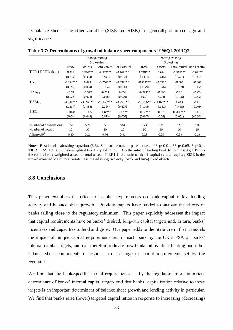
83
its balance sheet. The other variables (SIZE and RISK) are generally of mixed sign and
significance.
Table 3.7: Determinants of growth of balance sheet components 1996Q1-2011Q2
Notes: Results of estimating equation (3.8). Standard errors in parentheses; *** p<0.01, ** p<0.05, * p<0.1.
TIER 1 RATIO is the risk-weighted tier 1 capital ratio; TB is the ratio of trading book to total assets; RISK is
the ratio of risk-weighted assets to total assets; TIER1 is the ratio of tier 1 capital to total capital; SIZE is the
time-demeaned log of total assets. Estimated using two-way (bank and time) fixed effects .
3.8 Conclusions
This paper examines the effects of capital requirements on bank capital ratios, lending
activity and balance sheet growth. Previous papers have tended to analyse the effects of
banks falling close to the regulatory minimum. This paper explicitly addresses the impact
that capital requirements have on banks‘ desired, long-run capital targets and, in turn, banks‘
incentives and capacities to lend and grow. Our paper adds to the literature in that it models
the impact of unique capital requirements set for each bank by the UK‘s FSA on banks‘
internal capital targets, and can therefore indicate how banks adjust their lending and other
balance sheet components in response to a change in capital requirements set by the
regulator.
We find that the bank-specific capital requirements set by the regulator are an important
determinant of banks‘ internal capital targets and that banks‘ capitalization relative to these
targets is an important determinant of balance sheet growth and lending activity in particular.
We find that banks raise (lower) targeted capital ratios in response to increasing (decreasing)
RWA Assets Total capital Tier 1 capital RWA Assets Total capital Tier 1 capital
TIER 1 RATIO (kit-1) 0.416 0.864*** -8.327*** -0.367*** 1.249*** 0.674 -1.555*** -0.02***
(0.274) (0.334) (0.547) (0.031) (0.391) (0.416) (0.421) (0.007)
TBt-1 -0.264*** 0.038 -0.716*** -0.032*** -0.711*** -0.276* -0.004 -0.002
(0.052) (0.064) (0.104) (0.006) (0.129) (0.144) (0.139) (0.002)
RISKt-1 -0.03 -0.037 -0.012 0.001 -0.239** -0.094 0.2* >-0.001
(0.023) (0.028) (0.046) (0.003) (0.1) (0.14) (0.108) (0.002)
TIER1t-1 -4.388*** -3.592*** -18.457*** -0.955*** -10.256** -14.822*** 4.443 -0.03
(1.134) (1.384) (2.264) (0.127) (4.145) (4.391) (4.468) (0.079)
SIZEt-1 -0.028 -0.035 1.134*** 0.05*** -0.17*** -0.078 0.201*** 0.001
(0.04) (0.048) (0.079) (0.005) (0.047) (0.05) (0.051) (<0.001)
Number of observations 559 559 559 564 173 171 173 178
Number of groups 10 10 10 10 10 10 10 10
Adjusted R2 0.10 0.11 0.44 0.41 0.29 0.20 0.23 0.13
1996Q1-2006Q4 2007Q1-2011Q2
Growth in: Growth in:

84
capital requirements. To achieve these new targeted capital ratios, banks make adjustments
to capital and/or assets, including loans. These adjustments depend on the extent to which
banks‘ actual capital ratios differ from their revised target. We find evidence of a ―bank
capital channel‖ through which shocks to bank capitalization affect lending, balance sheet
and capital growth. This result is of interest to regulators trying to assess the potential
behavioural impact of new capital requirements. We also examine whether banks‘
adjustment of their balance sheet is different for a subset of banks that experience recent
changes in the capital requirements. We find that following a change in capital requirements,
banks tend to adjust their portfolios by altering the composition rather than the volume of
loans and other assets, for example by substituting towards lower risk-weighted assets. On
the capital side, banks tend to focus on relatively inexpensive, lower quality tier 2 capital,
rather than higher quality tier 1 capital. While based on a subset of our sample, these
findings indicate that under the Basel I prudential regime, banks tended to minimise the costs
of complying with capital requirements by adjusting lower quality capital and altering the
average risk weights of their portfolios.
Although these findings depend on a partial equilibrium view of banks‘ balance sheet
adjustment behaviour and do not take into account feedback effects from the real economy,
they are useful for highlighting shortcomings of the previous capital regime and for
illustrating the possible effects of proposals aimed at addressing such flaws. We use the
results to gauge the UK banking sector‘s response to a countercyclical capital requirement
similar to that proposed by the UK‘s FSA and included in the final Basel III package of
regulatory reforms. Our results provide evidence that banks, in an effort to alter capital
ratios, focus on raising the cheapest form of capital to the extent permitted by regulation as a
way of minimizing capital compliance costs. This finding raises questions about the efficacy
of countercyclical capital requirements if banks are able to satisfy higher capital requirements
with lower-quality, less loss absorbent capital elements. The evidence supports the current
emphasis in international discussions on raising the mandatory proportions of higher-quality
capital and using higher-quality capital as the basis for countercyclical capital requirements.
Finally, we have developed a simplified version of our model to test whether large banks
employed different approaches to adjusting towards target capital ratios in the post-crisis
period. Balance sheet adjustment is modelled in a single equation without an explicit role for
bank- and time-specific add-ons, which have played a secondary role in the crisis period. We
find that balance sheet adjustment in the crisis period tends to focus more on risk-weighted

85
assets and less on un-weighted assets in the crisis period, indicating that banks are more
likely to change the composition of their portfolios, or alter risk weights, than to contract
activities across the portfolio. We find a reduced role for adjustments in capital (total and tier
1) during the crisis, which may reflect low profitability and a high cost of raising external
funding during the crisis.

86
Chapter 4 : In Good Times and in Bad: Bank Capital Ratios and
Lending Rates
4.1 Introduction
The regulatory response to the late 2000s global financial crisis (GFC) includes substantially
higher bank capital requirements and a proposal for these requirements to vary
countercyclically, rising in boom conditions and falling in busts to dampen excess bank
procyclicality and smooth the credit cycle. These measures have fuelled an intense debate on
the macroeconomic impact of higher prudential standards. Estimates of the potential impact
of increased regulatory capital requirements on the cost of intermediation and the path of
economic growth vary greatly (Barrell et al, 2009; BCBS, 2010; Institute for International
Finance, 2010; Miles et al, 2011). Some studies refer to the Modigliani and Miller (1958)
capital structure theorems to argue that regulatory requirements have little impact on the
overall resource cost of bank intermediation (Admati et al, 2010; Kashyap et al, 2010; Miles
et al, 2011). This perspective contrasts with that of most practitioners who argue that the
higher capital requirements proposed under Basel III will substantially raise bank
intermediation costs and that this will pose difficulties for an already vulnerable real
economy.49
The empirical literature offers similarly conflicting evidence on the magnitude, and indeed
the direction, of the relationship between bank capital ratios and loan pricing. While cross-
country studies document a positive link between capital ratios and net interest margins
(Demirgüç-Kunt and Huizinga, 1999; Saunders and Schumacher, 2000; Carbó-Valverde and
Rodríguez-Fernández, 2007), studies utilizing data on individual country (mostly syndicated)
loans granted to large businesses find a negative relation (Hubbard et al, 2002; Steffen and
Wahrenburg, 2008; Santos and Winton, 2010). Time variation not accounted for in the
relation between bank capital and bank loan pricing could serve to rationalize this contrasting
evidence. One empirical study which supports this explanation is Fischer et al (2009) where a
negative relation between loan margins and the lender‘s capital ratio is documented using US
49
For instance, see financial press articles ‗We must rethink Basel, or growth will suffer‘ (Vikram Pandit,
Financial Times, 10th November 2010) and ‗Jamie Dimon says regulation will stifle economic growth‘ (Wall
Street Journal, 5th April 2011). Also see the impact assessment prepared by the Institute for International
Finance (2010).
87
individual loans over the period 1988-92, when regulatory changes and market pressure were
forcing bank capital ratios upwards, and a positive correlation during 1993-2005 when banks
operated in more benign conditions.
This paper seeks to contribute to the literature on the relation between bank capital and
lending with an examination of the 8 largest UK banks during the 14-year period 1998-2011.
Various aspects of our research strategy differentiate our work from existing studies. First,
the link between capital ratios and lending rates is explicitly broken down into a long-run co-
integrating relation and short-run dynamics of capital adjustment, whereas previous studies
conflate long- and short-run effects. We exploit a confidential regulatory dataset submitted by
banks to the Bank of England (BoE) and FSA which includes monthly effective interest rates
on loans and quarterly capital adequacy information. This allows us to depart from most
previous studies which rely on low-frequency annual data and hence, cannot distinguish
short-run and long-run effects. Second, our research investigates differences between the
pre-crisis period (‗good times‘) when there was little pressure on banks to increase capital
and the recent crisis period (‗bad times‘) when regulatory capital requirements have been
more consistent with market demands and hence, the cost of capital curve was less steep.
Our research strategy can be summarised as follows. An error correction modelling (ECM)
framework is adopted to estimate the long-run loan pricing relation. This ECM formulation is
able to capture short-run dynamic effects and controls for observed bank-level characteristics
such as the Tier 1 capital ratio and portfolio risk, system-wide indicators of the business cycle
such as the Bank of England base rate, market interest rates and the output gap, as well as
latent bank and time (i.e. two-way) fixed effects. In order to capture inter-temporal
differences in the relation caused by financial distress, we estimate a second model in which
the long-run effect is allowed to differ between the recent crisis period and earlier years.
Finally, we estimate a third model in which we replace the actual Tier 1 capital ratio with a
long-run target Tier 1 capital ratio proxy. This represents a more direct test of the potential
impact of capital requirements, since these achieve their affects by altering banks' own long-
run capital targets.
Our analysis finds no evidence for the positive long-run relation between capital ratios and
loan rates hypothesised during normal (i.e., pre-crisis) conditions. We interpret this as
evidence that bank funding costs were not much affected by capital ratios in this period. But
there is a clear difference between ‗good‘ and ‗bad‘ times: the link becomes significantly
88
negative, economically and statistically, in the crisis period. These findings are robust to
whether the actual capital ratio or the target capital ratio is used. We argue this is likely to
reflect the reduction in funding costs as banks‘ own optimal capital ratios rise due to
increased expected bankruptcy costs. In such conditions increases in capital ratios, generated
by regulatory and/or market pressures, tend to reduce funding costs (other things equal). We
also find a positive short-run relation between capital and lending rates, which becomes
stronger during the stressed period, supporting the idea that banks use interest margins as a
tool to increase their capital ratios under stress. Finally, we show that our results are robust
to controlling for banks' relative competitive positions (as proxied by market share).
These findings suggest that estimates of the impact of higher capital requirements on
lending rates and the broader economy should be analyzed in a framework that allows the
cost of capital requirements explicitly to vary over the business cycle and dynamically over
the long- and short-run. These findings also offer some insight into the use of
countercyclical bank capital requirements, as proposed in Basel III, as an additional tool to
constrain lending growth during booms and encourage lending during busts. It is difficult
directly to infer the effects of reductions in capital requirements during a crisis from our
sample, since in the recent financial crisis capital requirements were rising rather than
falling. However, our finding of a negative long-run link in stressed conditions provides
indirect evidence, since it suggests that in such conditions banks have an incentive to
increase their capital ratios and this in turn reduces their funding costs. This is consistent
with experience following the recent crisis when banks have raised capital ratios far more
than they have been required to by the transition to higher Basel III standards, which will
not be fully implemented until 2018. We conclude from this that the amplitude (i.e. the
range) of counter-cyclical variations in capital requirements needs to be very substantial
if they are to offset the cyclical contraction in lending that takes place under stressed
conditions.
The remainder of the paper is structured as follows. Section 4.2 discusses the
interrelationship between bank capital and loan interest rates, distinguishing three different
effects of bank capital on loan interest rates that we then go on to investigate empirically.
This section also reviews previous empirical literature on the relation between bank capital
and loan interest rates. Section 4.3 outlines our specification, methodology and data. Section
4.4 presents the estimation results. Section 4.5 concludes with a summary of our results and
their implications.

89
4.2 The interrelationship of bank capital and loan interest rates
4.2.1 Conceptual and theoretical background
The main goal of this paper is to estimate the relationship between bank capital and loan
interest rates, disentangling short-term dynamics and long-run effects and allowing for the
possibility that the balance of costs and benefits of holding bank capital (and hence, the
relationship with lending rates) alters substantially from one time period to another. While
this is mainly an empirical exercise, it is nonetheless important to provide some conceptual
and theoretical background.
It is crucial to be clear what is meant by bank capital. We distinguish between the capital
requirement which is the minimum capital ratio required by regulators, the capital ratio which
is the bank's actual capital ratio, and the long-run target capital ratio which is the level of
capital intended by the bank over the long run which can be defined as the capital
requirement plus the long-run desired capital buffer. Actual capital can differ from target
capital because of short-run adjustment costs. This target capital might be referred to as the
‗optimal capital ratio‘ but this terminology risks confusion with the ‗privately optimal capital
ratio‘, namely, the capital ratio that minimises funding costs and hence, would be optimal in
the absence of capital requirements. Finally, consistent with other studies, we use the term
capital buffer to refer to the excess of the actual capital ratio over the capital requirement.
This buffer is always positive or zero, except on rare occasions when firms are in breach of
regulatory requirements.
The empirical models formulated in this paper allow us to test three hypotheses about the
relationship between bank capital and loan interest rates:50
H1: Bank capital ratios and loan interest rates are positively related in the long run during
normal market conditions (Cost of Capital Effect)
H2: Under stressed market conditions, the long-run relation weakens or becomes negative
(Banking Sector Distress Effect)
50
For fuller reviews of the large theoretical literature on bank capital and its relationship with loan pricing see
Swank (1996), Bhattacharya and Thakor (1993) and VanHoose (2007).
90
H3: Banks use interest margins as a tool for managing actual capital ratios, implying that
there is a separate short-run link between bank capital and lending rates (Weak Bank Effect).
While we do not present a formal theoretical model, these three hypotheses seem to capture
most of the empirical predictions that emerge from various theories of bank capital. They can
be interpreted as follows. The first cost of capital hypothesis can be understood as a
prediction of standard capital structure theory. The basic Modigliani-Miller (MM)
propositions imply that changes in the funding mixture of firms will make no difference to
their funding costs. However, standard corporate finance theory suggests that capital market
frictions lead to a cost of capital curve that is U-shaped.51
First, debt interest payments tend
to be tax-deductible so that a lower capital ratio will reduce the tax bill and increase profits,
incentivising firms to hold more debt and less equity. On the other hand, expected
bankruptcy costs mean that, as the proportion of equity falls, the cost of funding rises, so that
a high probability of distress results in a higher cost of debt funding. In the classic trade-off
theory, these factors offset one another, producing an optimal capital ratio that minimises
funding costs. One alternative is the pecking order theory, in which adverse selection raises
the costs of issuing new equity, so that investment in new assets that cannot be financed out
of retained earnings will lower capital ratios (Myers and Majluf, 1984).
These theories are relevant to any firm. They have been applied to banks, for example, by
Miller (1995), Ellis and Flannery (1992), Flannery and Rangan (2006) and Mehran and
Thakor (2011). Banks have a number of features suggesting that they will be highly
leveraged relative to other firms (Berger et al, 1995). A classic theory of why financial
intermediaries exist is that they earn returns from the information they gather about
borrowers (Leland and Pyle, 1977; Diamond, 1984) and some argue that in the M-M setting
there is little rationale for banks to exist at all (Berger et al, 1995; Gambacorta and Mistrulli,
2004). In the pecking order theory, these agency problems imply that equity issuance may be
especially costly for banks (Holmstrom and Tirole, 1997; Stein, 1998). Implicit and explicit
state guarantees on banks‘ debt may also help explain why banks are highly leveraged
(Merton, 1977; Keeley, 1990; Berger et al, 1995).52
On the other hand, Mehran and Thakor
(2011) argue that the effect of expected bankruptcy costs could be particularly important for
51
A vast literature exists on the M-M theorems and we do not attempt to summarise it here. Comprehensive
reviews are provided by Myers (2001) and Brealey et al (2010) inter alios. 52
It is worth noting that the franchise value of a bank may act as a constraint on the incentives to maximise
leverage (Marcus, 1984; Keeley, 1990; Milne and Whalley, 2001).

91
banks, since a higher likelihood of bankruptcy reduces the bank‘s incentives to monitor
borrowers, implying that equity is positively associated with value, other things equal.
The implications of the trade-off view for a bank‘s cost of funding are shown in Figure 1, by
plotting the cost of funding (vertical axis) against the capital-asset ratio (horizontal axis). This
is intended as a graphical illustration rather than a formal model. The cost of funding curve
(CF1) is a plausible example to explain the key aspects of the trade-off view. As the capital
ratio falls, the cost of funding decreases linearly due to the tax and information advantages of
debt and the effects of state guarantees. When capital falls to low levels, expected
bankruptcy costs raise the cost of funding. Hence, our example illustrates that the sign and
magnitude of the relation between capital and the cost of funding depends on the level of
capital. In the absence of regulatory capital requirements, an optimising bank chooses A* as
target capital ratio where these factors just offset each other and the cost of funding is
minimised. .
Figure 4.1. Illustration of long-run cost of capital curve.
This figure illustrates the effects of capital structure on funding costs by plotting the weighted average cost of
funding (vertical axis) against the capital-asset ratio (horizontal axis). CF1 and CF2 denote the cost of funding
curves in normal and stressed market conditions, respectively. The shift from A* to  is thus the increase in the
target capital ratio from normal to stressed market conditions and the cost of funding increases from f1 to f3.
This shift from CF1 to CF2 and from A* to  could also be as the consequence of the imposition of capital
requirements. Â is the higher target capital ratio when there is a regulatory capital requirement. In normal
conditions imposing a capital requirement raises the cost of funding from f1 to f3, but if capital requirements are
imposed in stressed conditions the cost of funding remains at f3 since the bank‘s target capital ratio is the same
with or without capital requirements.
f1
f2
f3
A*
Â
Capital-asset ratio
Weig
hte
d a
vera
ge c
ost
of
fun
din
g
CF1
CF2
92
Figure 4.1 departs from many standard accounts because it does not present the regulatory
capital requirements as a continuously binding constraint, with an imposed level of capital
higher than the capital ratio A* (the target capital ratio in the absence of a capital
requirement) due to regulators‘ concern for the social as well as private costs of bank failure.
Instead this figure assumes that banks seek to hold a buffer over the capital requirement to
minimise the probability of unexpected breaches (Milne and Whalley, 2001). Regulatory
capital requirements alter the bank‘s target capital decision since falling below the capital
requirement imposes costs on the bank such as additional supervisory surveillance and limits
on the bank‘s activities. Due to these costs, a bank optimally chooses to hold a buffer over the
capital requirement to protect against unexpected and costly breaches.
In our illustrative graphical framework, imposing a capital requirement increases the bank‘s
target capital ratio to Â, which equals the capital requirement plus the bank‘s desired capital
buffer.53
Still, the empirical predictions of the standard analysis with binding regulatory
capital requirements and this buffer capital account are similar. Under the standard account,
without buffer capital, banks with binding capital requirements experience higher funding
costs and this, in turn, implies a positive link between capital and loan interest spreads
(Berger et al, 1995). In a setup that allows for buffer capital, a higher level of the capital
requirement that increases the bank's target level of capital implies a positive link in the long-
run between bank capital and loan interest spreads during normal market conditions. Note
that if capital requirements are to the left of the bank's own optimal capital ratio A* then they
are not binding, the bank chooses A*, and the relation between capital and funding costs is
flat.
Our second hypothesis is the less standard prediction that, in stressed market conditions, the
long-run relation between banks‘ capital ratios and loan interest rates may weaken (relative to
normal times) or be negative. This banking sector distress effect is driven by the observation
that banks tend to be under pressure from investors and other market participants to increase
capital ratios in crisis periods. When the banking system is in distress, banks with relatively
illiquid asset portfolios may be forced to deleverage by the high cost of refinancing their
debts (Cornett et al, 2011). Expected bankruptcy costs rise in periods of economic contraction
due to an increase in the probability of banks‘ illiquidity and insolvency distress, and lower
53
In the analysis above, we have made the simplifying assumption that the capital ratio demanded by the market
(depicted in the curves CF1 and CF2) is independent from the capital requirement imposed by regulators. In
practice, capital requirements are likely to influence investors‘ perceptions of bank riskiness.

93
expected profits reduce the value of the ―tax shield‖ provided by the tax deductibility of
interest expense. Thus in stressed market conditions, both the cost of funding and the target
bank capital ratio rise (Estrella, 2004; Hanson et al, 2010). For example, Berger (1995) offers
convincing evidence that widespread US bank failures and recession in the late 1980s caused
banks‘ optimal capital ratios to rise so that those with increased capital ratios paid lower rates
of return on their debt funding than other banks, and recorded higher profits as a result. An
influential recent advocacy of this view in relation to the recent financial crisis is Admati et al
(2010) who argue that much higher capital requirements are justified on the basis that risk
premia in banks‘ cost of funding will fall as a result of a reduction in the probability of
distress. Yang and Tsatsaronis (2012) present initial empirical support for such a notion,
finding that bank stock returns tend to be positively associated with business cycles and the
level of bank leverage. Hence, the normally positive long-run relation between capital ratios
and interest margins is likely to lessen or turn negative in stress scenarios.
This banking distress effect can also be explained through Figure 4.1. A downward shock to
the soundness of the banking sector increases expected bankruptcy costs and therefore shifts
the cost of funding curve to the north-east (from CF1 to CF2). To the right of  the upwards
slope of CF2 is less steep than that to the right of A* in CF1. Thus at the margin, small
increases in the capital requirement that cause the bank to hold capital ratios in excess of Â
do not impose costs (or only small ones) on the bank since this capital ratio is more consistent
with market demands.54
Increases in the capital requirement during stressed market
conditions are less costly than in normal conditions.
Assuming that a change in funding costs will be passed on to bank customers through deposit
and lending interest rates,55
this simple graphical illustration can be mapped into two of the
above hypotheses: the target capital ratio is positively correlated with the lending rate in the
long run (H1) and this relationship grows weaker during stressed market conditions (H2).
Our third hypothesis arises theoretically from the fact that the interest margin set by a bank is
not only a source of funds with which to remunerate investors, but it is also a source of new
capital via retained earnings (Milne, 2004; Santos and Winton, 2010) and it can be used to
54
It is possible that an increase in capital requirements would be associated with a decrease in the cost of
funding in the short run if it is consistent with market demands for higher capital. However, as Berger (1995)
points out, this should not be interpreted as support for the counter-intuitive notion that higher capital
requirements may reduce funding costs, since in time an optimising bank would increase its capital ratio anyway
to meet market demands. 55
Button et al (2010) document empirically the increase in funding costs of UK banks during the recent
financial crisis and assess its contribution to higher household lending rates.
94
manage the capital ratio via the denominator by influencing the supply of new credit. This
implies that the short-run relation between bank capital and lending rates differs from the
long-run relation as banks use interest margins for management of short-run deviations
(deficit/surplus) of capital from their long-run target capital. Higher loan margins allow a
bank to build up capital reserves and reduce growth of new credit, improving both the
denominator and numerator of the capital ratio. A weak bank will increase both its lending
rates and its capital ratio in the short run, and on this basis we expect that the short-run effect
of increases in lending rates on capital ratios, namely the weak bank effect, is positive.56
In contrast, some previous studies have argued that the weak bank effect is negative, since
downward shocks to a bank‘s capital ratio are accompanied by upward spikes in loan interest
rates as banks seek to strengthen their balance sheets by extracting a premium from their
customers (Hubbard et al, 2003; Steffen and Wahrenburg, 2008; Santos and Winton, 2010).
Whether a positive or a negative effect is observed is a matter of timing. If the shock is
recorded simultaneously with the adjustment of interest rates, as it would be in annual data
such as used by the studies cited above, it is more likely that we will observe a negative
relation. If the data separates the period in which the shock occurs from periods in which
lending rates and capital ratios adjust upwards, as higher frequency data such as ours would
do, a positive short-run effect is more likely to be observed. As we will argue below, it is
also more likely that the target capital ratio will be positively correlated with the lending rate
in the short run than the actual capital ratio, given that it will not reflect unplanned shocks to
the actual capital ratio.
Figure 4.2 below illustrates the short-run relation of bank capital with loan rates. On the
vertical axis we show the evolution in interest margin and capital ratio from time t0 to time t2
(rebased to use the same scale for simplicity). We first assume that the bank has a target
capital ratio which it seeks to maintain, defined as the capital requirement plus the desired
buffer. The term ―deviation‖ is used to refer to the short-run fluctuations of the capital ratio
around the bank‘s target capital ratio. This deviation can plausibly be negative (deficit) or
positive (surplus) whereas the capital buffer, which is the excess of the capital ratio over the
capital requirement, will almost always be positive (the so called ‗headroom‘ of banks).
56
For the sake of consistency with the previous literature we have used the terminology "weak bank effect" to
refer to this hypothesis. However, we note that this is equivalent to a "strong bank effect" whereby a bank cuts
interest margins in order to reduce its capital ratio, and this makes the same predictions in terms of the sign of
the short-run coefficients.

95
Figure 4.2: Illustration of short-run relation between capital and interest margins
Notes: The figure illustrates the potential short-run relation between the capital ratio (solid line), target capital
ratio (dashed line) and the interest margin (dotted line) over time (horizontal axis), with all series rebased to ease
comparison. The actual capital ratio equals the target capital ratio in the long run but deviations (surplus or
deficit) can be observed in the short term. In both panels the capital ratio is below the target capital ratio
implying a short-term deficit of capital.
At time t0 the capital ratio equals the target capital so the deviation is zero. An exogenous
negative shock to the capital ratio at t1 creates a short-term deficit (negative deviation) as
shown in Panel A. The bank responds by raising interest margins in order to rebuild its
balance sheet until actual capital reaches the long-run target capital path again at t2. This
illustrates the ambiguous direction of the short-run relation between actual capital ratio and
lending rates, since it is negative around t1 but later turns positive between t1 and t2. In Panel
B we show the effects of a sudden increase in capital requirements at time t1 which again
Time
A: Downward shock to actual capital ratio
B: Upward shock to target capital ratio
Time
Interest margin Capital ratio Target capital ratio
t 0 t 1 t 2
t 0 t 1 t 2

96
creates a short-term deficit of capital. Here the bank raises its interest margin in order to build
up capital, until the actual capital reaches the target capital ratio again at t2, and the interest
margin remains at a higher plateau in order to remunerate the higher capital ratio (consistent
with the cost of capital effect). In this case, the capital ratio and the interest margins will be
unambiguously positively related to one another in the short-run.
Furthermore, as Milne and Whalley (2001) show, if actual capital is reduced by an exogenous
shock such as an increase in capital requirements or unexpected loan losses, then the bank
may have an incentive to reduce risk quickly in order to avoid a costly breach of the capital
requirement. The resulting rebalancing of the portfolio towards less risky assets may reduce
loan interest rates, although to some extent this can be controlled for with a measure of
portfolio risk.
The short-run relation could confound observation of the long-run effect if not controlled for
properly. Hence, it is important to separate out short-run from long-run effects. To the best
of our knowledge, our study is the first attempt to do so. This may explain why extant
estimates of the relation between bank capital and interest margins (or interest rates), which
are summarised in the next section, are so conflicting in sign and/or magnitude. Given that
they use annual data and do not separate long- and short-run effects, either the weak bank
effect or the banking sector distress effect could explain the negative relation observed in
these studies, although they tend to acknowledge the weak bank effect only.
4.2.2 Previous empirical studies of bank capital and loan interest rates
Saunders and Schumacher (2000) analyse a large cross-country sample of banks for the
period 1988-95, and find that the capital-asset ratio is positively related to net interest
margins in most country-year combinations, which they explain using the cost of capital
effect described above. However, their findings are based on pure cross-section regressions
that do not jointly exploit the time series dimension of the data and thus cannot jointly model
short- and long-run effects. If capital ratios rise simultaneously in all banks in a particular
country, for example, due to higher capital requirements, the effect of capital on margins
would not be picked up in a cross-section regression. Hence, they may not capture the full
impact of the higher capital standards introduced by the original Basel Accord in this period.

97
Demirgüç-Kunt and Huizinga (1999) also use a large international sample of banks over the
period 1988-95 but, unlike the above study, the regression analysis exploits both the time-
and cross-section variation in the data to ascertain the role of the capital ratio and other
potential factors as drivers of net interest margins. However, their static panel regressions do
not explicitly control for a dynamic ―error correction‖ mechanism, namely, the catch up of
actual capital towards the long-run target path. Their findings suggest too that net interest rate
margins are significantly positively correlated with capital ratios although this relation is not
allowed to vary over time.
Another issue with the above two studies is that they adopt net interest rate margins (NIM) as
the dependent variable. This variable is calculated as interest revenue minus interest expense
over total assets, and it has an unfortunate property: a shift from debt to equity funding will
tend to increase the NIM even in the absence of any difference between the cost of the two
funding sources, since interest expense is included in the NIM but returns paid to
shareholders in the form of dividends are not. This effect lowers the signal-noise ratio by
making it hard to infer the relation between capital ratios and interest rates from the reported
relation between capital ratios and NIMs.
Carbó-Valverde and Rodríguez-Fernández (2007) use the interest spread, calculated as the
difference between lending and deposit rates, rather than the NIM. Their panel study of
European banks over the period 1994-2001 establishes that the capital-to-asset ratio is
strongly positively linked with the interest rate spread, although this effect is not permitted to
differ between banks or over time. Likewise, employing a large database of syndicated loans
issued by US borrowers over the period 1993-2007, Fischer et al (2009) find that the ratio of
total capital to risk-weighted assets is positively correlated with lending spreads.57
They
interpret this as evidence that borrowers prefer to do business with high capitalised banks and
that these banks can therefore extract a premium from borrowers. The cost of capital effect is
supported by these findings.
However, other studies using data on syndicated loans have found a negative relation
between interest margins and the capital ratio in both the US (Hubbard et al, 2002; Santos
and Winton, 2010) and the UK (Steffen and Wahrenburg, 2008). These results are attributed
57
The use of the risk-weighted capital ratio in Fischer et al 2009 could make it more difficult to uncover a
positive association given that higher portfolio risk will tend to reduce the capital ratio and raise the interest
spread, though we note that their regressions were also run using the equity-to-assets ratio and produced
qualitatively similar results. Nevertheless, we use the capital-asset ratio in our model of lending rates to avoid
this effect.

98
to the existence of the weak bank effect, namely, that banks with low capital ratios raise their
margins in order to repair their balance sheets and enable access to funding markets. It could
be that by not distinguishing between long- and short-run dynamics the studies cited above
find a negative relationship because the weak bank effect and cost of capital effect are then
entangled. A negative relation could also be due to a dominance of the banking sector
distress effect, i.e. banks reduce their cost of funding by raising capital ratios consistent with
market demands.
The latter rationale is implicit in the evidence from various papers cited above. Fischer et al
(2009) ran their regressions for the period 1987-92, similar to the sample period of Hubbard
et al (2002) and corresponding to the implementation of Basel I which raised regulatory
capital standards and forced increases for many banks. In contrast to their finding of a
positive relation for the period 1993-2005 which was noted above, they find a negative
relation for the earlier period, when banks were under pressure from regulators and the
market to raise capital ratios. In addition, Steffen and Wahrenburg (2008) find that a
negative relation only applies during economic downturns which may be periods in which
banks are under pressure to strengthen their balance sheets.
Various attempts have been made to measure the short-run impact of capital deficits on the
quantity of loans although, to the best of our knowledge, none of them use models that
explicitly control for long-run effects. Interest rates are one of the main tools by which banks
may seek to reduce loan supply, the others being credit rationing at existing interest rates
and/or tighter lending standards. Hence, such studies are likely to be consistent with a
negative short-run relation between deviations of the capital ratio from target and the interest
rate. For example, Francis and Osborne (2012) show that for UK banks experiencing a deficit
of capital relative to the long-run target capital ratio, growth in risk weighted assets is lower
and growth in capital higher as banks adjust their balance sheets to move back towards the
target capital ratio. Similarly, Berrospide and Edge (2010) show that US banks with capital
deficits tend to contract loan supply, and Gambacorta and Mistrulli (2004) find that the
imposition of bank-specific capital requirements on ―problem banks‖ in Italy can reduce
lending by up to 20%. The substantial literature on the impact of capital deficits in the US
during the late 1980s and early 1990s suggests that a contraction in lending supply is
99
associated with loan losses and higher capital requirements; although overall the inferences
on causality are mixed.58
Finally, few studies have tried to measure the long-run effect of higher bank capital
requirements on interest rates directly using market price data. Such estimates are obtained
by taking figures on the long-run return on debt and equity, then adding the extra costs of a
higher equity ratio to the interest charged to banks‘ customers in order to calculate the change
in the lending rate. Since the long-run return to equity tends to be larger than the return to
debt, these estimates naturally suggest a positive impact of capital on spreads. Furthermore, a
likely source of upward bias in such measures is that, as described above, the required returns
on equity and debt are likely to alter when expected bankruptcy costs are reduced. In
addition, banks are likely to exploit other ways of offsetting the additional cost, such as
reducing administrative expenses. Elliott (2009) concludes that the long-run impact of a one
percentage point increase in the ratio of equity to assets on the lending rate is likely to be
about 5-18 basis points. Kashyap et al (2010) put the range lower, at 2-6 basis points.
However, these studies make no attempt to jointly model long-run and short-run effects or to
assess how the impact of capital requirements on loan spreads may vary over the business
cycle. Both of these aspects differentiate our analysis from that conducted in previous
research.
One possible interpretation of the mixed findings is as follows. When the banking system is
weak and under pressure to raise capital, banks that have (or achieve) relatively high capital
ratios, and so are perceived as comparatively safe, enjoy relatively lower funding costs. They
may then use this opportunity to increase their market share, by lowering their loan rates
relative to market rates of interest. In other times, when investors are more relaxed about the
prospects of bankruptcy and banks are constrained by capital requirements, a more standard
cost of capital effect dominates, resulting in a positive relationship between capital and loan
rates.
Another potential explanation is that interest margins may be used as a source of capital or as
a lever to alter the supply of new credit in order to manage short-run deviations of actual
capital from the desired long-run target capital level. It is possible that long- and short-run
effects are to a large extent intertwined in existing estimates, since they do not allow for
dynamics in interest rate adjustment, and are based on low-frequency annual data.
58
See comprehensive reviews by Jackson et al (1999) and Sharpe (1995).

100
4.3 Methodology, Data and Variables
4.3.1 Description of data and variables
We use confidential data submitted by banks to the FSA and the BoE. Banks authorised in
the UK (except foreign branches) are required to submit detailed data to the FSA on a
quarterly basis on their balance sheets and capital adequacy, first through the Banking
Supervision Database and since 2008 through the FSA‘s GABRIEL (Gathering Better
Regulatory Information Electronically) system. The forms have been changed several times
during our sample period, which limits the number of consistently defined variables available
to us. However, we are able to obtain a complete quarterly dataset of risk-weighted and un-
risk-weighted capital ratios for the period 1998-2011.
Our data on effective interest rates comes from returns submitted by large retail banks to the
BoE on a monthly basis over the period 1998-2011. Banks submit the average loan balances
and the interest received, net of arrears, for each month, enabling the calculation of monthly
effective interest rates (using the RIR and ER forms). Banks also submit the total write-offs
in the monthly returns (on the WO form). The BoE collect this data with the primary aim of
assessing the transmission of monetary policy, and consequently they apply cost-benefit
analysis to restrict the sample to a small number of large banks by which the returns must be
submitted. In addition, the criteria for entering the sample underwent a substantial overhaul
in 2004, resulting in a discontinuity in the sample at this point. We therefore only retain in
our sample banks which report both before and after the beginning of 2004 in order to avoid
sample selection effects.
The analysis is based on observations for the 8 largest UK commercial banks over the period
1998-2011. Our monthly sample59
for the individual estimation of the ECM specification
(Step 2) comprises a maximum of T=148 months from October 1998 to June 2011. The
sample is unbalanced with a maximum T of 148 months and a minimum of 126 months.
59
One practical issue we face is that the frequency of the observations on actual capital ratios (kit), the output
gap (gt) and write-offs (rit) is quarterly, but those on the rest of the covariates such as loan rates (lit), the base rate
(bt) and spread of 1-year LIBOR over the base rate (ft) are monthly. Thus the quarterly variables are converted
to monthly using linear interpolation so that they can be incorporated into the monthly ECM Equation (4.3).
Our quarterly panel for estimating the target capital Equation (4.4) is unbalanced but most banks are observed
over the entire period 1998Q4-2011Q2; the average (median) number of quarters is 44 (50) ranging from 26 to a
maximum of 50.
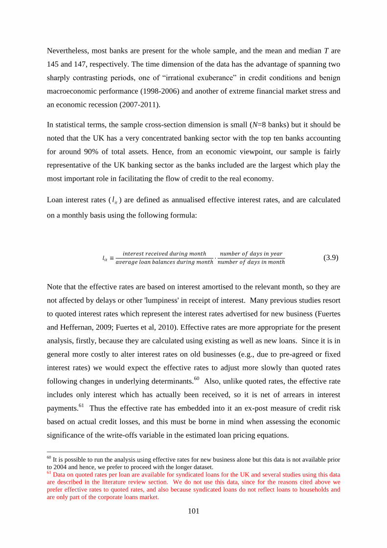
101
Nevertheless, most banks are present for the whole sample, and the mean and median T are
145 and 147, respectively. The time dimension of the data has the advantage of spanning two
sharply contrasting periods, one of ―irrational exuberance‖ in credit conditions and benign
macroeconomic performance (1998-2006) and another of extreme financial market stress and
an economic recession (2007-2011).
In statistical terms, the sample cross-section dimension is small (N=8 banks) but it should be
noted that the UK has a very concentrated banking sector with the top ten banks accounting
for around 90% of total assets. Hence, from an economic viewpoint, our sample is fairly
representative of the UK banking sector as the banks included are the largest which play the
most important role in facilitating the flow of credit to the real economy.
Loan interest rates ( itl ) are defined as annualised effective interest rates, and are calculated
on a monthly basis using the following formula:
𝑙𝑖𝑡 ≡𝑖𝑛𝑡𝑒𝑟𝑒𝑠𝑡 𝑟𝑒𝑐𝑒𝑖𝑣𝑒𝑑 𝑑𝑢𝑟𝑖𝑛𝑔 𝑚𝑜𝑛𝑡
𝑎𝑣𝑒𝑟𝑎𝑔𝑒 𝑙𝑜𝑎𝑛 𝑏𝑎𝑙𝑎𝑛𝑐𝑒𝑠 𝑑𝑢𝑟𝑖𝑛𝑔 𝑚𝑜𝑛𝑡∙𝑛𝑢𝑚𝑏𝑒𝑟 𝑜𝑓 𝑑𝑎𝑦𝑠 𝑖𝑛 𝑦𝑒𝑎𝑟
𝑛𝑢𝑚𝑏𝑒𝑟 𝑜𝑓 𝑑𝑎𝑦𝑠 𝑖𝑛 𝑚𝑜𝑛𝑡 (3.9)
Note that the effective rates are based on interest amortised to the relevant month, so they are
not affected by delays or other 'lumpiness' in receipt of interest. Many previous studies resort
to quoted interest rates which represent the interest rates advertised for new business (Fuertes
and Heffernan, 2009; Fuertes et al, 2010). Effective rates are more appropriate for the present
analysis, firstly, because they are calculated using existing as well as new loans. Since it is in
general more costly to alter interest rates on old businesses (e.g., due to pre-agreed or fixed
interest rates) we would expect the effective rates to adjust more slowly than quoted rates
following changes in underlying determinants.60
Also, unlike quoted rates, the effective rate
includes only interest which has actually been received, so it is net of arrears in interest
payments.61
Thus the effective rate has embedded into it an ex-post measure of credit risk
based on actual credit losses, and this must be borne in mind when assessing the economic
significance of the write-offs variable in the estimated loan pricing equations.
60
It is possible to run the analysis using effective rates for new business alone but this data is not available prior
to 2004 and hence, we prefer to proceed with the longer dataset. 61
Data on quoted rates per loan are available for syndicated loans for the UK and several studies using this data
are described in the literature review section. We do not use this data, since for the reasons cited above we
prefer effective rates to quoted rates, and also because syndicated loans do not reflect loans to households and
are only part of the corporate loans market.
102
Under the international regulatory framework established by the Basel Committee for
Banking Supervision (BCBS), total regulatory capital is set at a minimum of 8% of the
bank‘s risk-weighted assets. Regulatory capital has two components: i) Tier 1 capital which
consists of common equity, reserves and certain hybrid equity-like securities, and ii) Tier 2
capital which consists of subordinated debt and other permitted debt instruments. Total
regulatory capital is then calculated as the sum of Tier 1 and eligible Tier 2 capital (Tier 2
must be less than 50% of the total) less certain required deductions such as intangible assets
and investments in subsidiaries. In our analysis, we only use the Tier 1 capital ratio. The
reasons for this are two-fold. Firstly, Tier 2 is equivalent, economically speaking, to
subordinated debt funding and will therefore have a similar required rate of return to such
junior debt.62
Altering the amount of Tier 2 capital is therefore unlikely to be very costly and
so, since our hypotheses are based on the idea that capital is loss-absorbing and therefore
affects the cost of funding, Tier 2 capital is irrelevant to our analysis. Secondly, Tier 1
capital is now of more interest to regulators than total capital given that Tier 2 capital proved
to be ineffective in stemming a loss of confidence in banks during the financial crisis.
In order to calculate the risk-weighted assets, which constitute the denominator of the capital
requirement, the bank‘s assets are multiplied by risk weights which are set to capture the
level of risk that the bank is exposed to. In the standardized-weights approach prescribed by
the Basel I framework from 1989-2006, assets are allocated into a number of risk ―buckets‖
and then added together with pre-specified weights. Basel II, introduced in the UK in 2007,
permits and encourages banks to use, with approval from the supervisor, their own internal
models to measure credit risk (and, in turn, the risk weight) of each loan. An additional
component of risk-weighted assets is the trading book in which market risk is incorporated
through the Value-at-Risk approach. Reviews of Basel II aimed at addressing further issues
and shortfalls are ongoing (see footnote 64), although a floor to the Basel II rules based on
Basel I was in force in the European Union from 2007 and beyond the end of our sample
period.
The above regulatory setting has been superseded as additional measures were introduced in
the aftermath of the late 2000s GFC. From 2008, Tier 1 capital ratios rose substantially as
the FSA set higher benchmark expectations for firms in the context of the government
62
See FSA Consultation Paper Strengthening Capital Standards 2 (2006) for relevant pre-crisis estimates of the
required rate of return on different types of regulatory capital.

103
support package for major banks.63
In 2010, the Basel Committee announced new
international capital standards which raised the minimum Tier 1 requirement from 8% of
risk-weighted assets to 11%.64
Though these will not take effect immediately (on current
plans, they will be phased in by 2018), they have come to be seen as benchmark minima by
the market and many banks are targeting the future requirements now in order to prove their
resilience to the market or to satisfy supervisors.65
4.3.2 Empirical strategy
Our analysis unfolds in three sequential steps. First, we estimate a loan pricing equation
which aims to disentangle short- and long-run effects via an error correction modelling
(ECM) methodology. Second, we re-estimate the model allowing the long- and short-run
effects of banks' capital ratios to differ between normal and crisis periods. Thirdly, we re-
estimate the loan pricing equation using an estimated long-run target capital ratio measure in
place of the observed actual capital ratio. Finally, we extend our analysis to investigate the
role of market share as an additional determinant of loan margins.
Step 1: Estimating loan pricing equations using an error-correction model
In the first step we estimate a loan pricing equation following the error correction modelling
(ECM) framework adopted by Fuertes et al (2009, 2010) for analyzing the long-run relation
between UK retail bank interest rates and the BoE base rate. We extend their ECM by
considering other control variables such as capital ratios and portfolio risk. This framework is
adopted since it allows us to separately identify the short- and long-run effects of bank capital
ratios on lending rates.
63
Formally, this was not an increase in capital requirements. In the context of the package of bailout and
guarantees announced in the autumn of 2008 following the disastrous collapse of Lehman Brothers, the FSA
announced that the benchmark expectations following the package would be a Tier 1 capital ratio of 8% and
core Tier 1 of 4% following deduction of losses associated with a hypothetical stress scenario. Clearly, the
consequences of breaching these expectations imply that banks may in practice have treated them as higher
capital requirements. 64
See the first consultative document on the new Basel III package, December 2009,
http://www.bis.org/publ/bcbs164.htm, and press release from the Basel Committee on Banking Supervision
announcing agreed calibration, September 2010, http://www.bis.org/press/p100912.pdf. 65
The interim report of the Institute of International Finance (2010) summarises possible reasons for banks‘
adjustment to Basel III standards ahead of formal implementation.
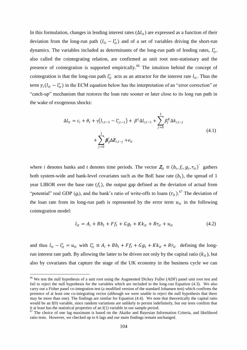
104
In this formulation, changes in lending interest rates (∆𝑙𝑖𝑡 ) are expressed as a function of their
deviation from the long-run path (𝑙𝑖𝑡 − 𝑙𝑖𝑡∗ ) and of a set of variables driving the short-run
dynamics. The variables included as determinants of the long-run path of lending rates, 𝑙𝑖𝑡∗ ,
also called the cointegrating relation, are confirmed as unit root non-stationary and the
presence of cointegration is supported empirically.66
The intuition behind the concept of
cointegration is that the long-run path 𝑙𝑖𝑡∗ acts as an attractor for the interest rate 𝑙𝑖𝑡 . Thus the
term 𝛾𝑖(𝑙𝑖𝑡 − 𝑙𝑖𝑡∗ ) in the ECM equation below has the interpretation of an ―error correction‖ or
―catch-up‖ mechanism that restores the loan rate sooner or later close to its long run path in
the wake of exogenous shocks:
∆𝑙𝑖𝑡 = 𝑐𝑖 + 𝜃𝑡 + γ 𝑙𝑖 ,𝑡−1 − 𝑙𝑖 ,𝑡−1
∗ + 𝛽𝐿Δ𝑙𝑖,𝑡−1 + 𝛽𝑗𝐾∆𝑘𝑖,𝑡−𝑗
1
𝑗=0
+ 𝜷𝒋′∆Z𝑖 ,𝑡−𝑗
1
𝑗=0
+𝑒𝑖𝑡
(4.1)
where i denotes banks and t denotes time periods. The vector Z𝑖𝑡 ≡ 𝑏𝑡 ,𝑓𝑡 ,𝑔𝑡 , 𝑟𝑖𝑡 ′ gathers
both system-wide and bank-level covariates such as the BoE base rate (𝑏𝑡), the spread of 1
year LIBOR over the base rate (𝑓𝑡), the output gap defined as the deviation of actual from
―potential‖ real GDP (gt), and the bank‘s ratio of write-offs to loans (𝑟𝑖𝑡).67
The deviation of
the loan rate from its long-run path is represented by the error term 𝑢𝑖𝑡 in the following
cointegration model:
𝑙𝑖𝑡 = 𝐴𝑖 + 𝐵𝑏𝑡 + 𝐹𝑓𝑡 + 𝐺𝑔𝑡 + 𝐾𝑘𝑖𝑡 + 𝑅𝑟𝑖𝑡 + 𝑢𝑖𝑡 (4.2)
and thus 𝑙𝑖𝑡 − 𝑙𝑖𝑡∗ = 𝑢𝑖𝑡 with 𝑙𝑖𝑡
∗ ≡ 𝐴𝑖 + 𝐵𝑏𝑡 + 𝐹𝑓𝑡 + 𝐺𝑔𝑡 + 𝐾𝑘𝑖𝑡 + 𝑅𝑟𝑖𝑡 defining the long-
run interest rate path. By allowing the latter to be driven not only by the capital ratio (𝑘𝑖𝑡 ), but
also by covariates that capture the stage of the UK economy in the business cycle we can
66
We test the null hypothesis of a unit root using the Augmented Dickey Fuller (ADF) panel unit root test and
fail to reject the null hypothesis for the variables which are included in the long-run Equation (4.3). We also
carry out a Fisher panel co-integration test (a modified version of the standard Johansen test) which confirms the
presence of at least one co-integrating vector (although we were unable to reject the null hypothesis that there
may be more than one). The findings are similar for Equation (4.4). We note that theoretically the capital ratio
would be an I(0) variable, since random variations are unlikely to persist indefinitely, but our tests confirm that
it at least has the statistical properties of an I(1) variable in our sample period. 67
The choice of one lag maximum is based on the Akaike and Bayesian Information Criteria, and likelihood
ratio tests. However, we checked up to 6 lags and our main findings remain unchanged.
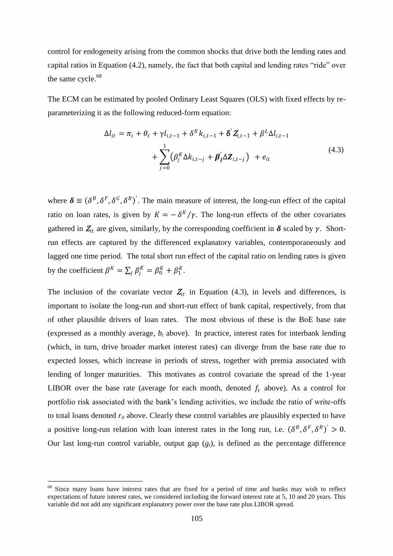
105
control for endogeneity arising from the common shocks that drive both the lending rates and
capital ratios in Equation (4.2), namely, the fact that both capital and lending rates ―ride‖ over
the same cycle.68
The ECM can be estimated by pooled Ordinary Least Squares (OLS) with fixed effects by re-
parameterizing it as the following reduced-form equation:
∆𝑙𝑖𝑡 = 𝜋𝑖 + 𝜃𝑡 + γ𝑙𝑖 ,𝑡−1 + 𝛿𝐾𝑘𝑖 ,𝑡−1 + δ′Z𝑖,𝑡−1 + 𝛽𝐿Δ𝑙𝑖,𝑡−1
+ 𝛽𝑗𝐾Δ𝑘𝑖 ,𝑡−𝑗 + 𝜷𝒋
′∆𝒁𝑖 ,𝑡−𝑗
1
𝑗=0
+ 𝑒𝑖𝑡 (4.3)
where 𝜹 ≡ 𝛿𝐵 ,𝛿𝐹 , 𝛿𝐺 , 𝛿𝑅 ′ . The main measure of interest, the long-run effect of the capital
ratio on loan rates, is given by 𝐾 = −𝛿𝐾 𝛾 . The long-run effects of the other covariates
gathered in Z𝑖𝑡 are given, similarly, by the corresponding coefficient in 𝜹 scaled by 𝛾. Short-
run effects are captured by the differenced explanatory variables, contemporaneously and
lagged one time period. The total short run effect of the capital ratio on lending rates is given
by the coefficient 𝛽𝐾 = 𝛽𝑗𝐾
𝑗 = 𝛽0𝐾 + 𝛽1
𝐾 .
The inclusion of the covariate vector Z𝑖𝑡 in Equation (4.3), in levels and differences, is
important to isolate the long-run and short-run effect of bank capital, respectively, from that
of other plausible drivers of loan rates. The most obvious of these is the BoE base rate
(expressed as a monthly average, bt above). In practice, interest rates for interbank lending
(which, in turn, drive broader market interest rates) can diverge from the base rate due to
expected losses, which increase in periods of stress, together with premia associated with
lending of longer maturities. This motivates as control covariate the spread of the 1-year
LIBOR over the base rate (average for each month, denoted 𝑓𝑡 above). As a control for
portfolio risk associated with the bank‘s lending activities, we include the ratio of write-offs
to total loans denoted rit above. Clearly these control variables are plausibly expected to have
a positive long-run relation with loan interest rates in the long run, i.e. 𝛿𝐵 ,𝛿𝐹 , 𝛿𝑅 ′ > 0.
Our last long-run control variable, output gap (gt), is defined as the percentage difference
68
Since many loans have interest rates that are fixed for a period of time and banks may wish to reflect
expectations of future interest rates, we considered including the forward interest rate at 5, 10 and 20 years. This
variable did not add any significant explanatory power over the base rate plus LIBOR spread.
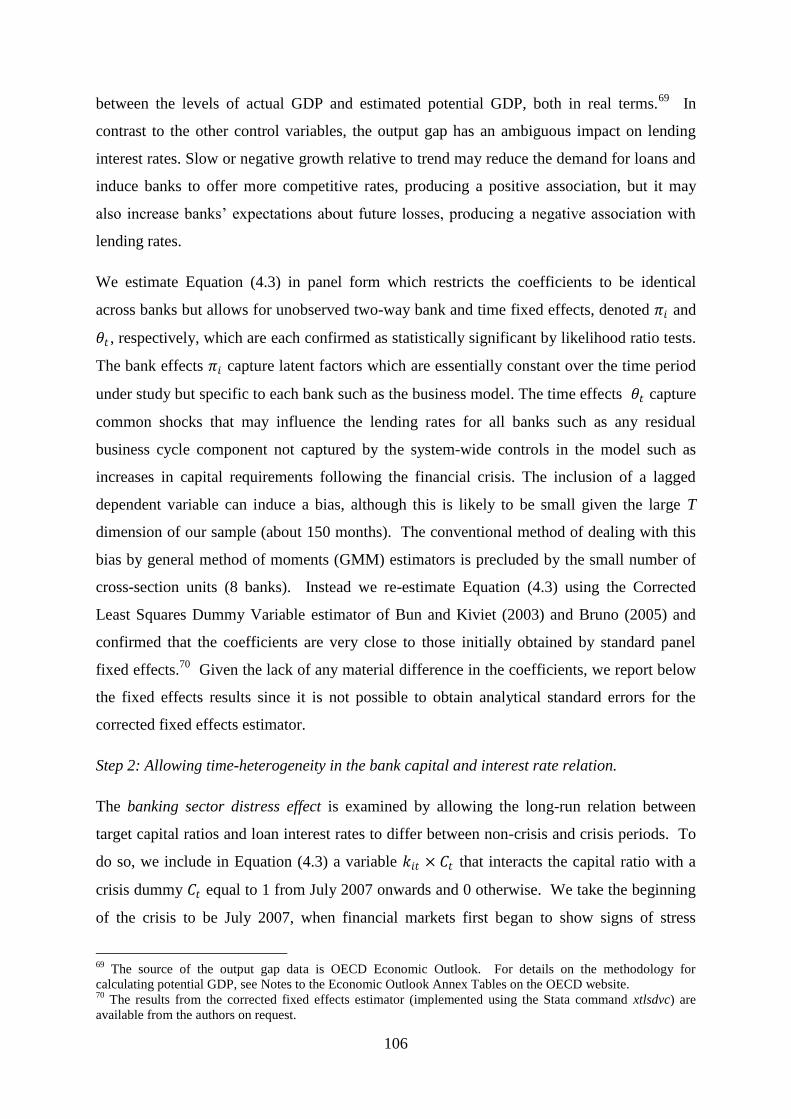
106
between the levels of actual GDP and estimated potential GDP, both in real terms.69
In
contrast to the other control variables, the output gap has an ambiguous impact on lending
interest rates. Slow or negative growth relative to trend may reduce the demand for loans and
induce banks to offer more competitive rates, producing a positive association, but it may
also increase banks‘ expectations about future losses, producing a negative association with
lending rates.
We estimate Equation (4.3) in panel form which restricts the coefficients to be identical
across banks but allows for unobserved two-way bank and time fixed effects, denoted 𝜋𝑖 and
𝜃𝑡 , respectively, which are each confirmed as statistically significant by likelihood ratio tests.
The bank effects 𝜋𝑖 capture latent factors which are essentially constant over the time period
under study but specific to each bank such as the business model. The time effects 𝜃𝑡 capture
common shocks that may influence the lending rates for all banks such as any residual
business cycle component not captured by the system-wide controls in the model such as
increases in capital requirements following the financial crisis. The inclusion of a lagged
dependent variable can induce a bias, although this is likely to be small given the large T
dimension of our sample (about 150 months). The conventional method of dealing with this
bias by general method of moments (GMM) estimators is precluded by the small number of
cross-section units (8 banks). Instead we re-estimate Equation (4.3) using the Corrected
Least Squares Dummy Variable estimator of Bun and Kiviet (2003) and Bruno (2005) and
confirmed that the coefficients are very close to those initially obtained by standard panel
fixed effects.70
Given the lack of any material difference in the coefficients, we report below
the fixed effects results since it is not possible to obtain analytical standard errors for the
corrected fixed effects estimator.
Step 2: Allowing time-heterogeneity in the bank capital and interest rate relation.
The banking sector distress effect is examined by allowing the long-run relation between
target capital ratios and loan interest rates to differ between non-crisis and crisis periods. To
do so, we include in Equation (4.3) a variable 𝑘𝑖𝑡 × 𝐶𝑡 that interacts the capital ratio with a
crisis dummy 𝐶𝑡 equal to 1 from July 2007 onwards and 0 otherwise. We take the beginning
of the crisis to be July 2007, when financial markets first began to show signs of stress
69
The source of the output gap data is OECD Economic Outlook. For details on the methodology for
calculating potential GDP, see Notes to the Economic Outlook Annex Tables on the OECD website. 70
The results from the corrected fixed effects estimator (implemented using the Stata command xtlsdvc) are
available from the authors on request.
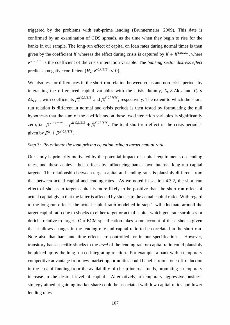
107
triggered by the problems with sub-prime lending (Brunnermeier, 2009). This date is
confirmed by an examination of CDS spreads, as the time when they begin to rise for the
banks in our sample. The long-run effect of capital on loan rates during normal times is then
given by the coefficient 𝐾 whereas the effect during crisis is captured by 𝐾 + 𝐾𝐶𝑅𝐼𝑆𝐼𝑆 , where
𝐾𝐶𝑅𝐼𝑆𝐼𝑆 is the coefficient of the crisis interaction variable. The banking sector distress effect
predicts a negative coefficient (H2: 𝐾𝐶𝑅𝐼𝑆𝐼𝑆 < 0).
We also test for differences in the short-run relation between crisis and non-crisis periods by
interacting the differenced capital variables with the crisis dummy, 𝐶𝑡 × Δk𝑖𝑡 and 𝐶𝑡 ×
Δk𝑖 ,𝑡−1 with coefficients 𝛽0𝐾,𝐶𝑅𝐼𝑆𝐼𝑆
and 𝛽1𝐾,𝐶𝑅𝐼𝑆𝐼𝑆
, respectively. The extent to which the short-
run relation is different in normal and crisis periods is then tested by formulating the null
hypothesis that the sum of the coefficients on these two interaction variables is significantly
zero, i.e. 𝛽𝐾,𝐶𝑅𝐼𝑆𝐼𝑆 = 𝛽0𝐾,𝐶𝑅𝐼𝑆𝐼𝑆 + 𝛽1
𝐾,𝐶𝑅𝐼𝑆𝐼𝑆 . The total short-run effect in the crisis period is
given by 𝛽𝐾 + 𝛽𝐾,𝐶𝑅𝐼𝑆𝐼𝑆 .
Step 3: Re-estimate the loan pricing equation using a target capital ratio
Our study is primarily motivated by the potential impact of capital requirements on lending
rates, and these achieve their effects by influencing banks' own internal long-run capital
targets. The relationship between target capital and lending rates is plausibly different from
that between actual capital and lending rates. As we noted in section 4.3.2, the short-run
effect of shocks to target capital is more likely to be positive than the short-run effect of
actual capital given that the latter is affected by shocks to the actual capital ratio. With regard
to the long-run effects, the actual capital ratio modelled in step 2 will fluctuate around the
target capital ratio due to shocks to either target or actual capital which generate surpluses or
deficits relative to target. Our ECM specification takes some account of these shocks given
that it allows changes in the lending rate and capital ratio to be correlated in the short run.
Note also that bank and time effects are controlled for in our specification. However,
transitory bank-specific shocks to the level of the lending rate or capital ratio could plausibly
be picked up by the long-run co-integrating relation. For example, a bank with a temporary
competitive advantage from new market opportunities could benefit from a one-off reduction
in the cost of funding from the availability of cheap internal funds, prompting a temporary
increase in the desired level of capital. Alternatively, a temporary aggressive business
strategy aimed at gaining market share could be associated with low capital ratios and lower
lending rates.

108
In order to isolate the effects of target capital, we re-estimate Equation (4.3) replacing the
actual capital ratio 𝑘𝑖𝑡 with a proxy for the long-run target capital ratio 𝑘𝑖𝑡∗ level around which
the former fluctuates, i.e. 𝑘𝑖𝑡 ≡ 𝑘𝑖𝑡∗ + 휀𝑖𝑡 where 휀𝑖𝑡 is a zero mean innovation representing
random temporary fluctuations of the bank‘s actual capital around its long-run target capital
level. The long-run target capital ratio is defined as the fitted values of the following auxiliary
regression for quarterly data:
𝑘𝑖𝑡 = 𝛼𝑖 + 𝜗𝑡 + 𝜷′X𝑖𝑡 + 휀𝑖𝑡 (4.4)
where Xit is a the 31 vector of covariates comprising the ratio of risk-weighted assets to total
assets, the ratio of corporate loans to total loans and the ratio of trading book assets to total
assets.71
Equation (4.4) is also estimated by fixed effects allowing for unobserved bank-
specific factors αi and time effects 𝜗𝑡 .72
We compute the target risk-weighted capital ratio for each bank and time quarter as the fitted
values 𝛼 𝑖 + 𝜷 ′X𝑖𝑡 + 𝝑 𝒕 multiplied by the ratio of risk-weighted assets to total assets. The
resulting measure denoted 𝑘𝑖𝑡∗ represents the un-weighted target capital-to-assets ratio (or the
target ―leverage ratio‖ in standard regulatory jargon) that is used in the subsequent analysis as
the bank‘s long-term target capital. The reason for converting the risk-weighted ratio into a
target leverage ratio is that the former conflates the effects of portfolio risk and capitalization
in a way that is unhelpful for our analysis, and therefore it is preferable to separate out the
effects of portfolio risk and capitalization.
Step 4: Extension to consider market structure
Finally, we extend our analysis to examine the effects of market structure. One might
intuitively argue that banks with a more dominant market position will have higher lending
71
The return on equity is often included in capital structure regressions (see section 2.1 and Chapter 5).
However, unfortunately it is unavailable in our sample since income statement data was not collected regularly
for much of our sample period. 72
Previous research has shown that bank- and time-varying capital requirements imposed by the FSA in excess
of the Basel minimum 8% are significant determinants of the total (i.e. Tier 1 + Tier 2) capital ratio (Francis and
Osborne, 2012). We tested whether this is also true of the Tier 1 capital ratio. The relation was not significant in
the pre-crisis period, implying that banks chose Tier 1 capital according to internal targets and then adjusted
Tier 2 capital to meet regulatory total capital requirements (this is consistent with detailed analysis of capital
adjustment in Francis and Osborne (2012)). In the crisis period, an implausibly large coefficient is observed
implying that changes in the capital ratio were several multiples of changes in capital requirements. We believe
this could be attributed to simultaneous market and regulatory pressure on banks‘ capital ratios during the crisis.
These issues imply that capital requirements are not necessarily good predictors of target Tier 1 capital ratios
and hence we do not use them in our model of long-run target capital.

109
rates and be more able to alter lending rates without altering market share. To the extent that
the competitive position of each bank is time constant, the mark-up will be captured by the
bank fixed effects 𝜋𝑖 in our loan pricing Equation (4.3). However, Equation (4.3) does not
allow the bank‘s competitive position to vary over time, and it also does not allow the long-
run and short-run effects of capital on the lending rate to vary according to the competitive
position of each bank. As a check on this, we re-estimate Equation (4.3) with two additional
covariates in Zit, one consisting of the bank‘s loans divided by total lending by UK financial
institutions as a simple proxy for a bank‘s competitive position denoted 𝑀𝑖𝑡 , with long-run
coefficient and an interaction between market share and actual capital, 𝑘𝑖𝑡 × 𝑀𝑖𝑡 with
long-run coefficient denoted and short-run coefficient denoted 𝛽𝑘 ,𝑀 .
4.4 Empirical results
We begin by providing summary statistics of the main covariates in our analysis. We then
discuss inferences on the long-run and short-run effects hypothesized in Section 4.2.1.
4.4.1 Descriptive statistics
Four main variables in our analysis, regulatory Tier 1 capital ratio (aggregated across banks),
lending rates (aggregated), the BoE base rate and the 1-year LIBOR rate are plotted in Figure
4.3. The path of the base rate, 𝑏𝑡 , is well-known: following a period until 2007 in which it
moves only by small amounts to counteracting movements in inflation, it then drops down to
an historic low of 0.5% in 2008 and remains there until the end of our sample in 2011. The
lending rate, 𝑙𝑖𝑡 averaged across i=1,…,8 large UK banks, exhibits a broadly similar long-run
path albeit it does not fall as much as the base rate in 2008, which implies incomplete interest
rate pass-through. Button et al (2010) provide a discussion of possible reasons for the
significant widening of the spread between lending rates and the base rate observed from
2008 onwards. It may reflect higher credit risk as the credit quality of borrowers deteriorates
and banks require larger risk premia to compensate. It may also be because banks were
trying to repair their balance sheets by raising capital via margins, partly to offset the losses
incurred during the crisis and partly in response to tighter regulatory standards. Over the
same period, the output gap drops substantially during 2008-2009 and stays negative
henceforth, suggesting that increased loan margins may be explained in part by the economic
contraction following the financial crisis, which may have affected banks‘ estimates of
expected arrears as well as their desire to build up their capital as a cushion for future losses.

110
Figure 4.3: Trends in UK capital ratios and lending rate.
Notes: The figure plots the monthly evolution 1998:10-2011:06 in the ratio of Tier 1 capital to assets (aggregate
across banks), the lending rate (aggregate across banks), the Bank of England base rate, and the 1-year LIBOR
rate. All variables correspond to the left vertical axis. Quarterly Tier 1 ratios are mapped into monthly figures
using linear interpolation. The aggregated Tier 1 ratio and lending rate are calculated by adding stocks and flows
over all banks in the sample at each time period.
Figure 4.3 also shows that the increase in the spread over base rate occurs roughly at the same
time as a substantial increase in the aggregate actual Tier 1 capital ratio, 𝑘𝑖𝑡 , across i = 1,…,8
banks; the latter more than doubles from 2% in early 2008 to 5.5% in mid 2011. These trends
are consistent with an increase in the cost of funding accompanying higher capital ratios. It is
also possible that they are influenced by other factors, for example, an increase in the cost of
debt associated with a higher probability of bank distress, as suggested by the widening
spread of 1-year LIBOR over base rate during the same period, or higher loan losses resulting
from the late 2000s recession.
In order to choose the period for our crisis dummy in equation (4.3), we analysed CDS prices
for the banks in our sample since these are likely to reflect investor sentiment about each
bank. We calculate an average price for each bank based on 1 year and 5 year maturities and
senior and subordinated debt and compute an index by dividing the CDS price by the average
price over the pre-crisis period 2004-06. The CDS indices for each bank, shown in Figure
4.4 below, sharply increase from July 2007 onwards, coinciding with public concerns about
the valuation of structured products and a drying up of the market for short-term asset-backed
0%
1%
2%
3%
4%
5%
6%
7%
8%
9%
Tier capital / assets Lending rate
Base rate 1 year LIBOR
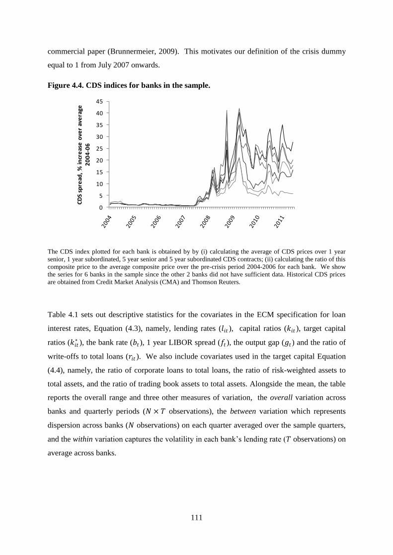
111
commercial paper (Brunnermeier, 2009). This motivates our definition of the crisis dummy
equal to 1 from July 2007 onwards.
Figure 4.4. CDS indices for banks in the sample.
The CDS index plotted for each bank is obtained by by (i) calculating the average of CDS prices over 1 year
senior, 1 year subordinated, 5 year senior and 5 year subordinated CDS contracts; (ii) calculating the ratio of this
composite price to the average composite price over the pre-crisis period 2004-2006 for each bank. We show
the series for 6 banks in the sample since the other 2 banks did not have sufficient data. Historical CDS prices
are obtained from Credit Market Analysis (CMA) and Thomson Reuters.
Table 4.1 sets out descriptive statistics for the covariates in the ECM specification for loan
interest rates, Equation (4.3), namely, lending rates (𝑙𝑖𝑡 ), capital ratios (𝑘𝑖𝑡 ), target capital
ratios (𝑘𝑖𝑡∗ ), the bank rate (𝑏𝑡), 1 year LIBOR spread (𝑓𝑡), the output gap (𝑔𝑡) and the ratio of
write-offs to total loans (𝑟𝑖𝑡 ). We also include covariates used in the target capital Equation
(4.4), namely, the ratio of corporate loans to total loans, the ratio of risk-weighted assets to
total assets, and the ratio of trading book assets to total assets. Alongside the mean, the table
reports the overall range and three other measures of variation, the overall variation across
banks and quarterly periods (𝑁 × 𝑇 observations), the between variation which represents
dispersion across banks (𝑁 observations) on each quarter averaged over the sample quarters,
and the within variation captures the volatility in each bank‘s lending rate (𝑇 observations) on
average across banks.
0
5
10
15
20
25
30
35
40
45
CD
S sp
read
, %
incr
eas
e o
ver
ave
rage
2
00
4-0
6

112
Table 4.1. Summary statistics for bank-specific covariates in loan pricing ECM
equation.
Source Mean Range Standard deviation
Overall Between Within
Monthly variables
(T=151)
Lending rate (lit) BOE/FSA 6.5 1.9 - 10 1.6 0.8 1.4
Bank rate (bt) Datastream 4.0 0.5 - 6.4 1.8 - -
1y LIBOR spread (ft) Datastream 0.1 -4.5 - 3.9 2.3 - -
Quarterly variables
(T=51)
Output gap (gt) Datastream 0.5 -0.7 - 1.7 0.5 - -
Tier 1 capital ratio (𝑘𝑖𝑡 ) BOE/FSA 4.0 1.3 - 8.6 1.3 0.8 1.1
Target capital (𝑘𝑖𝑡∗
) BOE/FSA 4.0 1.5 - 9.1 1.2 0.8 1.0
Write-offs/loans (rit) BOE/FSA 0.9 0.1 - 11.1 1.1 0.8 0.9
Corporate loans/loans BOE/FSA 22.7 0 - 61.7 15.1 14.9 6.5
RWA/assets BOE/FSA 45.0 8.9 - 76.7 14.2 10.5 10.2
TB assets/assets BOE/FSA 14.7 0 - 64.4 16.7 15.9 7.5
Notes: All variables are reported in percentages. The monthly and quarterly observations span the same period,
i.e. 1998:10-2011:06, and 1998:Q4-2001Q2, respectively, for the 8 largest UK banks. Lending rate is annualised
loan interest received over average loan balances in each month. Bank rate is a monthly average of the base
interest rate set by the Bank of England and 1y LIBOR spread is the difference between the 1 year LIBOR
interest rate and the bank rate. The output gap is the quarterly deviation of output from potential output
calculated by the OECD. Tier 1 capital ratio is the ratio of Tier 1 capital to total assets. Target capital ratio is the
fitted values from Equation (4.4) estimated by two-way fixed effects and subsequently un-weighted. Annualised
write-offs of loans are expressed as a proportion of loans. Corporate loans are expressed as a percentage of total
loans. Risk-weighted assets (RWA) are expressed as a percentage of total assets. Trading book (TB) assets are
expressed as a percentage of total assets. The quarterly variables that appear in the ECM Equation (4.3) (output
gap, capital ratios, write-offs/loans) are mapped to monthly data by linear interpolation.
113
4.4.2 Tests of hypothesis on the relation between capital ratio and loan rates
The estimation results of the loan interest rate ECM Equation (4.3) using monthly data are set
out in Table 4.2. For the sake of brevity, we focus the discussion on the parameters of
interest, namely, the long-run coefficients (B, F, G, K and R) and the short-run coefficient on
the covariate representing deviations of actual capital from target capital (𝛽𝐾). The results of
our base specification are shown in column (1); we then show the results of interacting the
capital ratio with a crisis interaction variable in column (2), and finally in column (3) we re-
run the specification in column (2) replacing the actual capital ratio with the long-run target
capital ratio.
The results make interesting reading. First, the long-run coefficient of the bank‘s capital ratio
(K) is negative in the base model shown in column (1) and this coefficient is both statistically
and economically highly significant. This is in contrast to the cost of capital effect which
predicts that maintaining higher capital ratios will raise the cost of funding and therefore
drive higher lending rates in the long run. Since our sample period includes both a benign
period and a period of acute distress, it is possible that the negative relation observed on
average across the sample period could be driven by the banking sector distress effect
dominating in the crisis period. We test this in column (2), which separates the long-run
coefficient on the capital ratio into a base effect (K) corresponding to normal or ‗good times‘
and a crisis period effect (K+ KCRISIS
) corresponding to ‗bad times‘. Our results are
consistent with the banking sector distress effect. The interaction effect KCRISIS
is negative
and economically large in magnitude as well as highly statistically significant. In contrast,
the long-run link between capital ratios and loan rates in good times, measured by K, is far
smaller and statistically insignificant.
In terms of our theoretical analysis of the long-run relation in Section 4.2.1, the lack of a
significant link between capital ratios and lending rates in the pre-crisis period indicates that
banks on average may be close to their privately optimal capital ratios where increasing or
decreasing the capital ratio has little or no effect on the cost of funding. This further
suggests that Tier 1 capital requirements may not have been binding on banks during the pre-
crisis period.73
The lack of binding capital requirements may explain why we do not find a
73
A notion that is given additional support by the lack of significant correlation between Tier 1 capital
requirements and capital ratios in this period (see footnote 72)
114
positive relation consistent with the cost of capital effect, since this hypothesis relies on banks
being on the upwards-sloping part of the cost of funding curve where they are being forced to
hold more capital than they would choose for themselves. In contrast, the strongly negative
long-run relation observed for the crisis period suggests that in this period, optimal capital
ratios may have increased so that banks that increased their capital ratios reduced their
funding costs (other things equal) and passed this on to their borrowers via a lower cost of
funding, consistent with the banking sector distress effect.
Next in order to obtain the results shown in column (3) of Table 4.2, we need first to
approximate the long-run target capital level 𝑘𝑖𝑡∗ which will then replace the actual Tier 1
capital ratio 𝑘𝑖𝑡 in the loan interest rate ECM Equation (4.3). As noted above, we do this in
order to isolate the effects of bank capital targets, since these are likely to be closer to the
effects of capital requirements which achieve their aims by influencing banks‘ own internal
capital targets. We estimated the target capital ratio as described in Section 4.3.2 via
Equation (4.4). The coefficients for the ratio of risk-weighted assets to total assets, the share
of corporate loans in total loans and the ratio of trading book assets to total assets were -0.17,
0.11 and -0.08 respectively, and all of these were significant at the 5% level or better. The
ratio of risk-weighted assets to total assets (i.e., risk ratio) is negatively linked with the capital
ratio. Prima facie this result is surprising as it implies that riskier business models have lower
long-term target capital ratios ceteris paribus, but it is probably due to the fact that the capital
ratio has already been adjusted using appropriate risk weights. Hence, the negative coefficient
of the risk ratio covariate reflects that riskier banks tend to hold less capital against a given
set of risk assets. The capital ratio varies positively with the proportion of corporate loans in
total loans, suggesting that this is an indicator of riskier business models. The ratio of trading
book assets to total assets is negatively related to the capital ratio, suggesting that banks
choose to hold less capital against trading book activities, plausibly because these are more
actively hedged than banking book assets. Finally, we plot the estimated time-effects 𝜗𝑡 from
the reduced-form target capital ratio Equation (4.4) in Figure 4.5 below. Reassuringly, these
estimates confirm that capital ratios rose simultaneously and sharply across the banks in our
sample following the onset of the crisis in late 2007, which can be attributed to regulatory
and market pressure and decline in the demand for loans.
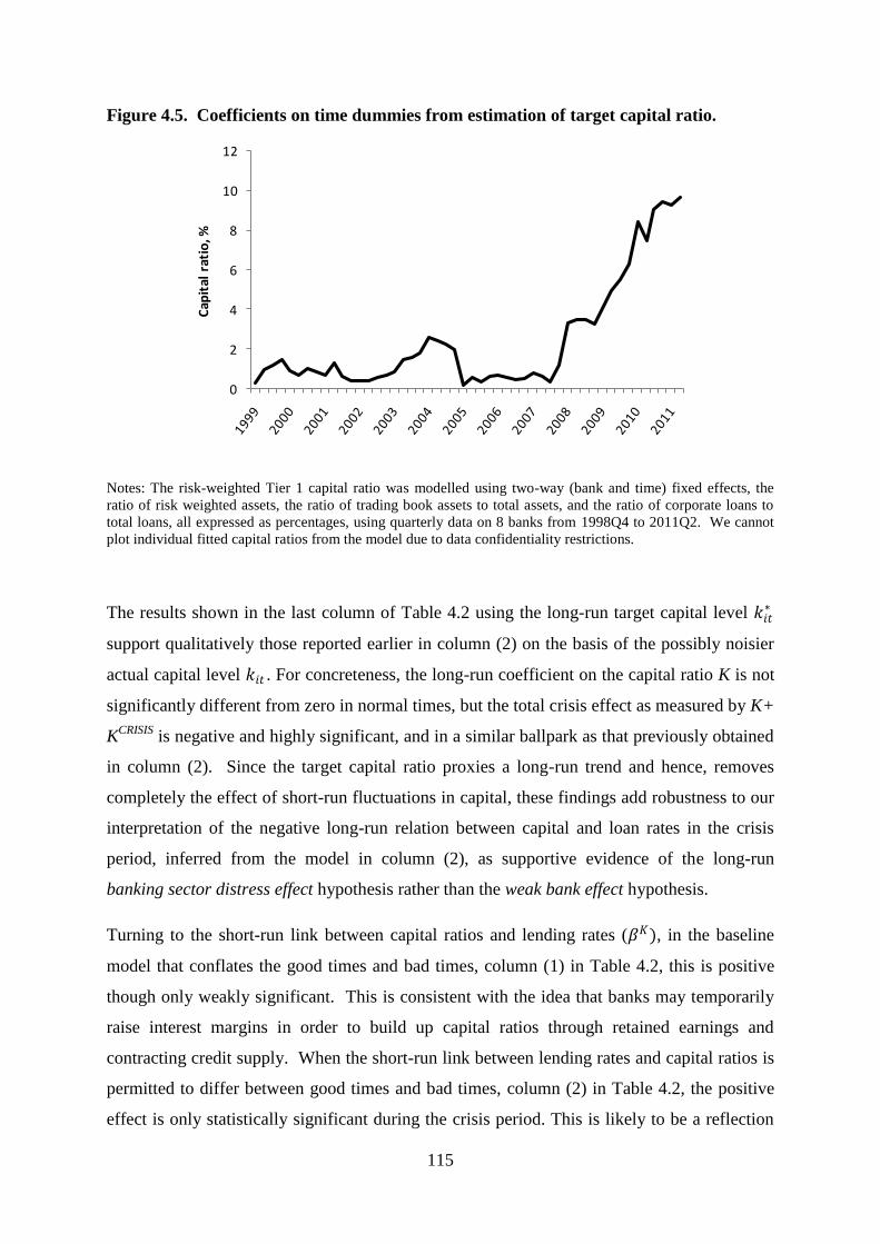
115
Figure 4.5. Coefficients on time dummies from estimation of target capital ratio.
Notes: The risk-weighted Tier 1 capital ratio was modelled using two-way (bank and time) fixed effects, the
ratio of risk weighted assets, the ratio of trading book assets to total assets, and the ratio of corporate loans to
total loans, all expressed as percentages, using quarterly data on 8 banks from 1998Q4 to 2011Q2. We cannot
plot individual fitted capital ratios from the model due to data confidentiality restrictions.
The results shown in the last column of Table 4.2 using the long-run target capital level 𝑘𝑖𝑡∗
support qualitatively those reported earlier in column (2) on the basis of the possibly noisier
actual capital level 𝑘𝑖𝑡 . For concreteness, the long-run coefficient on the capital ratio K is not
significantly different from zero in normal times, but the total crisis effect as measured by K+
KCRISIS
is negative and highly significant, and in a similar ballpark as that previously obtained
in column (2). Since the target capital ratio proxies a long-run trend and hence, removes
completely the effect of short-run fluctuations in capital, these findings add robustness to our
interpretation of the negative long-run relation between capital and loan rates in the crisis
period, inferred from the model in column (2), as supportive evidence of the long-run
banking sector distress effect hypothesis rather than the weak bank effect hypothesis.
Turning to the short-run link between capital ratios and lending rates (𝛽𝐾), in the baseline
model that conflates the good times and bad times, column (1) in Table 4.2, this is positive
though only weakly significant. This is consistent with the idea that banks may temporarily
raise interest margins in order to build up capital ratios through retained earnings and
contracting credit supply. When the short-run link between lending rates and capital ratios is
permitted to differ between good times and bad times, column (2) in Table 4.2, the positive
effect is only statistically significant during the crisis period. This is likely to be a reflection
0
2
4
6
8
10
12
Cap
ital
rat
io, %
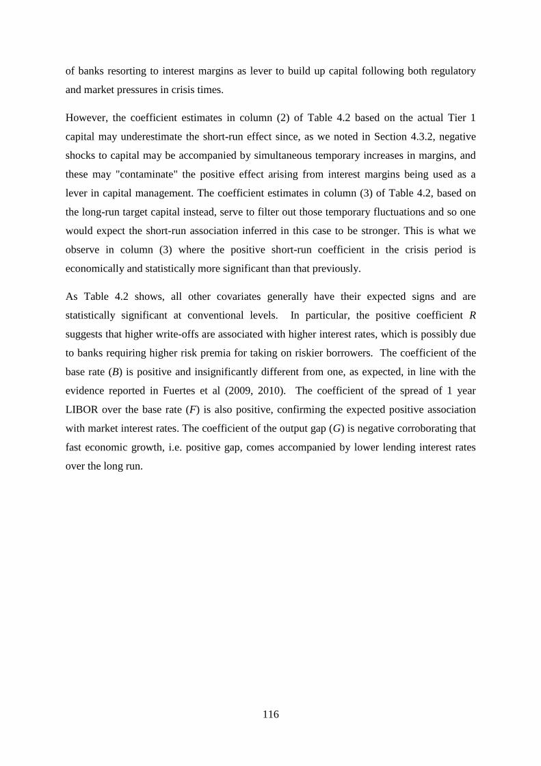
116
of banks resorting to interest margins as lever to build up capital following both regulatory
and market pressures in crisis times.
However, the coefficient estimates in column (2) of Table 4.2 based on the actual Tier 1
capital may underestimate the short-run effect since, as we noted in Section 4.3.2, negative
shocks to capital may be accompanied by simultaneous temporary increases in margins, and
these may "contaminate" the positive effect arising from interest margins being used as a
lever in capital management. The coefficient estimates in column (3) of Table 4.2, based on
the long-run target capital instead, serve to filter out those temporary fluctuations and so one
would expect the short-run association inferred in this case to be stronger. This is what we
observe in column (3) where the positive short-run coefficient in the crisis period is
economically and statistically more significant than that previously.
As Table 4.2 shows, all other covariates generally have their expected signs and are
statistically significant at conventional levels. In particular, the positive coefficient R
suggests that higher write-offs are associated with higher interest rates, which is possibly due
to banks requiring higher risk premia for taking on riskier borrowers. The coefficient of the
base rate (B) is positive and insignificantly different from one, as expected, in line with the
evidence reported in Fuertes et al (2009, 2010). The coefficient of the spread of 1 year
LIBOR over the base rate (F) is also positive, confirming the expected positive association
with market interest rates. The coefficient of the output gap (G) is negative corroborating that
fast economic growth, i.e. positive gap, comes accompanied by lower lending interest rates
over the long run.

117
Table 4.2. Estimation of loan interest rate ECM equation 1998:10-2011:06.
Notes: Monthly observations on 8 large UK banks are used to estimate the ECM Equation (4.3), using two-way
(bank and time) fixed effects. K is the long-run coefficient of the bank‘s capital ratio (𝑘𝑖𝑡) or target capital ratio
(𝑘𝑖𝑡∗ ), KCRISIS
is the coefficient of the target capital ratio interacted with a crisis dummy variable equal to 1 from
July 2007 onwards and 0 otherwise, B is the long-run coefficient of the monthly average policy rate set by the
Bank of England (bt), R is the long-run coefficient of the annualized loans write-offs over total loans (rit), F is
the long-run coefficient of the spread of 1-year LIBOR over base rate (ft), G is the long-run coefficient of the
output gap (gt). The dependent variable for these long-run coefficients is the lending rate, defined as annualised
loan interest received over average loan balances in each month. 𝛽𝐾 is the short-run coefficient of the capital
ratio calculated as the sum of coefficients on the first difference and lagged first difference of the capital ratio
(Δ𝑘𝑖𝑡 and Δ𝑘𝑖 ,𝑡−1), 𝛽𝐾,𝐶𝑅𝐼𝑆𝐼𝑆 is the short-run coefficient interacted with a crisis dummy variable equal to 1 from
July 2007 onwards and 0 otherwise. The dependent variable for these short-run coefficients is the change in
the lending rate. We also show total short-run and long-run effects of capital in the crisis (i.e., K+KCRISIS
and
𝛽𝐾+𝛽𝐾,𝐶𝑅𝐼𝑆𝐼𝑆 ). The target capital ratios used in column (3) are estimated on quarterly data via two-way fixed
effects and then converted to un-risk-weighted capital ratios, as described above. All variables are expressed as
percentages. Standard errors are in parentheses. *, ** and *** denote significance at the 10%, 5% and 1%
levels, respectively.
(1) (2) (3)
Using actual capital
ratio
Using actual capital
ratio, with crisis
interaction dummy
Using target capital
ratio, with crisis
interaction dummy
B Base rate 1.35*** 0.93* 1.23
(0.43) (0.47) (0.75)
F 1-year LIBOR spread 1.9** 0.76 -0.06
(0.83) (1.39) (1.53)
R Write-offs/loans 0.22* 0.29** 0.43***
(0.13) (0.12) (0.11)
G Output gap -0.63 -0.69* -1.1**
(0.4) (0.38) (0.48)
K Capital ratio -0.33*** -0.07 -0.25
(0.11) (0.13) (0.18)
KCRISIS Capital ratio x crisis dummy -0.4** -0.12
(0.16) (0.18)
K+KCRISIS Total -0.46*** -0.36***
(0.13) (0.14)
βK 0.1* 0.04 0.13
(0.05) (0.08) (0.14)
βK,CRISIS 0.1 0.37**
(0.09) (0.15)
βK+β
K,CRISIS 0.14** 0.5***
(0.07) (0.13)
No. of observations 1184 1184 1172
No. of banks 8 8 8
R-squared
- within 0.42 0.42 0.41
- between 0.41 0.26 0.18
- overall 0.38 0.38 0.38
Dependent variable = Lit
Dependent variable = ∆Lit
Long-run coefficients
Short-run coefficients
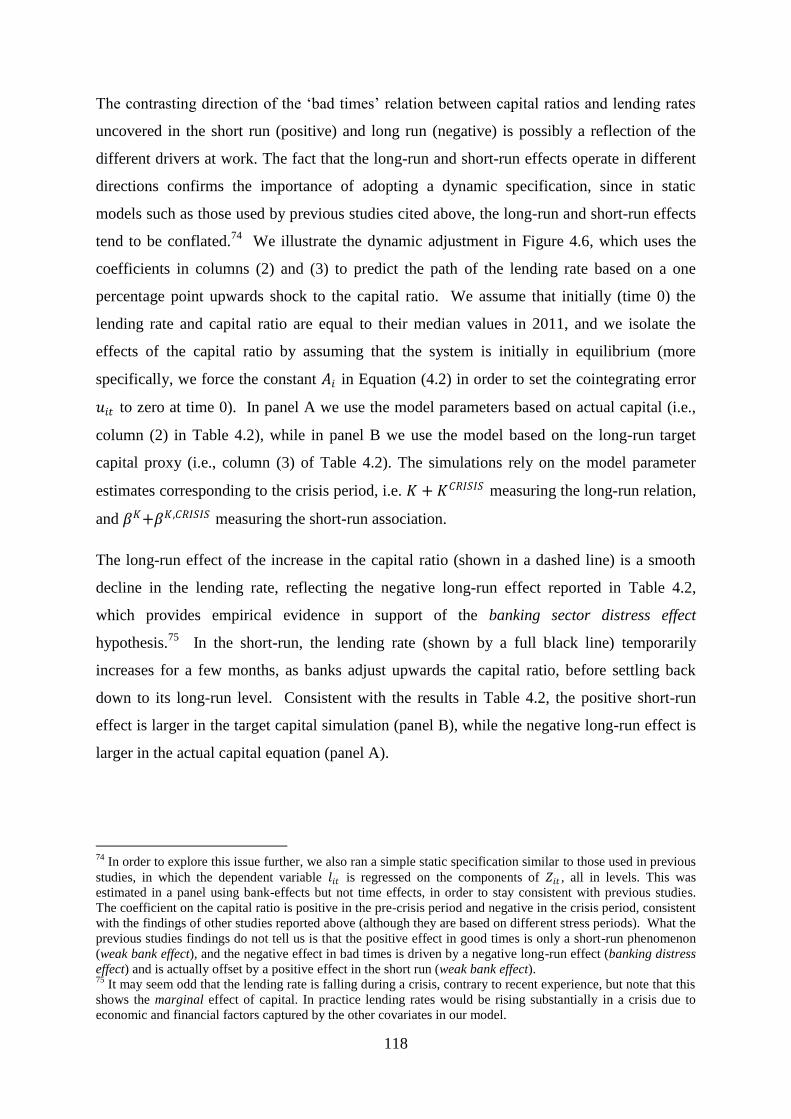
118
The contrasting direction of the ‗bad times‘ relation between capital ratios and lending rates
uncovered in the short run (positive) and long run (negative) is possibly a reflection of the
different drivers at work. The fact that the long-run and short-run effects operate in different
directions confirms the importance of adopting a dynamic specification, since in static
models such as those used by previous studies cited above, the long-run and short-run effects
tend to be conflated.74
We illustrate the dynamic adjustment in Figure 4.6, which uses the
coefficients in columns (2) and (3) to predict the path of the lending rate based on a one
percentage point upwards shock to the capital ratio. We assume that initially (time 0) the
lending rate and capital ratio are equal to their median values in 2011, and we isolate the
effects of the capital ratio by assuming that the system is initially in equilibrium (more
specifically, we force the constant 𝐴𝑖 in Equation (4.2) in order to set the cointegrating error
𝑢𝑖𝑡 to zero at time 0). In panel A we use the model parameters based on actual capital (i.e.,
column (2) in Table 4.2), while in panel B we use the model based on the long-run target
capital proxy (i.e., column (3) of Table 4.2). The simulations rely on the model parameter
estimates corresponding to the crisis period, i.e. 𝐾 + 𝐾𝐶𝑅𝐼𝑆𝐼𝑆 measuring the long-run relation,
and 𝛽𝐾+𝛽𝐾,𝐶𝑅𝐼𝑆𝐼𝑆 measuring the short-run association.
The long-run effect of the increase in the capital ratio (shown in a dashed line) is a smooth
decline in the lending rate, reflecting the negative long-run effect reported in Table 4.2,
which provides empirical evidence in support of the banking sector distress effect
hypothesis.75
In the short-run, the lending rate (shown by a full black line) temporarily
increases for a few months, as banks adjust upwards the capital ratio, before settling back
down to its long-run level. Consistent with the results in Table 4.2, the positive short-run
effect is larger in the target capital simulation (panel B), while the negative long-run effect is
larger in the actual capital equation (panel A).
74
In order to explore this issue further, we also ran a simple static specification similar to those used in previous
studies, in which the dependent variable 𝑙𝑖𝑡 is regressed on the components of 𝑍𝑖𝑡 , all in levels. This was
estimated in a panel using bank-effects but not time effects, in order to stay consistent with previous studies.
The coefficient on the capital ratio is positive in the pre-crisis period and negative in the crisis period, consistent
with the findings of other studies reported above (although they are based on different stress periods). What the
previous studies findings do not tell us is that the positive effect in good times is only a short-run phenomenon
(weak bank effect), and the negative effect in bad times is driven by a negative long-run effect (banking distress
effect) and is actually offset by a positive effect in the short run (weak bank effect). 75
It may seem odd that the lending rate is falling during a crisis, contrary to recent experience, but note that this
shows the marginal effect of capital. In practice lending rates would be rising substantially in a crisis due to
economic and financial factors captured by the other covariates in our model.
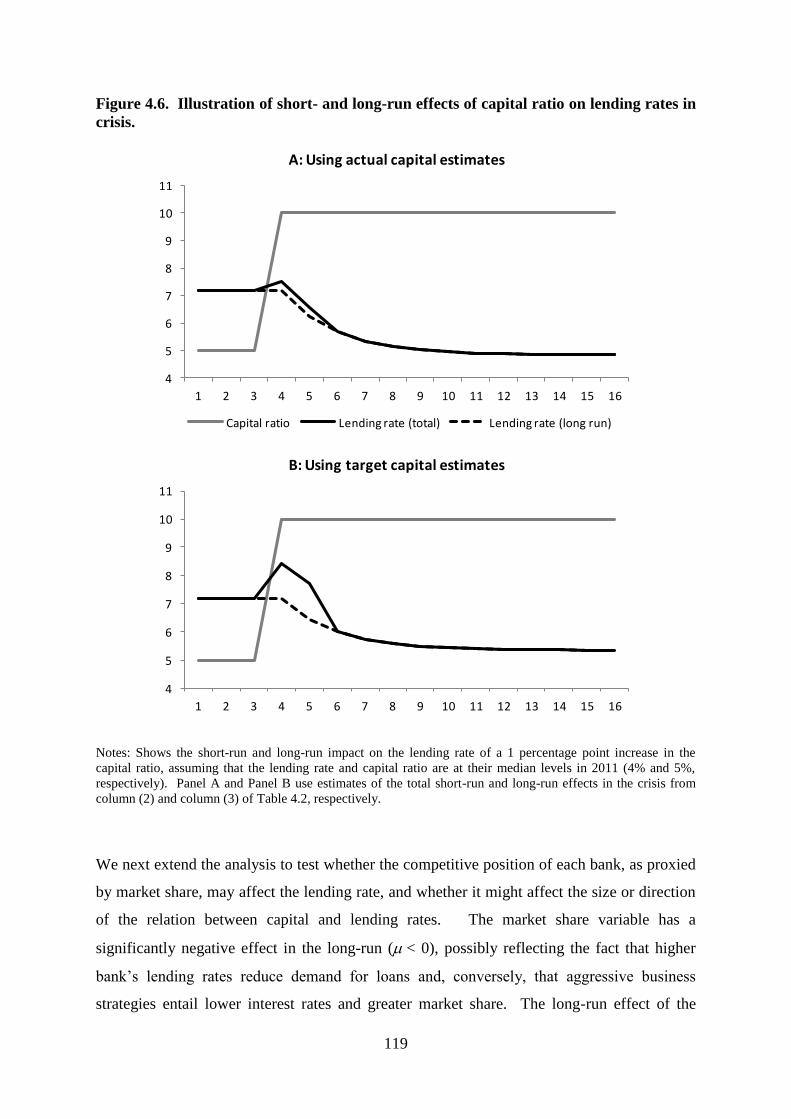
119
Figure 4.6. Illustration of short- and long-run effects of capital ratio on lending rates in
crisis.
Notes: Shows the short-run and long-run impact on the lending rate of a 1 percentage point increase in the
capital ratio, assuming that the lending rate and capital ratio are at their median levels in 2011 (4% and 5%,
respectively). Panel A and Panel B use estimates of the total short-run and long-run effects in the crisis from
column (2) and column (3) of Table 4.2, respectively.
We next extend the analysis to test whether the competitive position of each bank, as proxied
by market share, may affect the lending rate, and whether it might affect the size or direction
of the relation between capital and lending rates. The market share variable has a
significantly negative effect in the long-run (< 0), possibly reflecting the fact that higher
bank‘s lending rates reduce demand for loans and, conversely, that aggressive business
strategies entail lower interest rates and greater market share. The long-run effect of the
4
5
6
7
8
9
10
11
1 2 3 4 5 6 7 8 9 10 11 12 13 14 15 16
A: Using actual capital estimates
Capital ratio Lending rate (total) Lending rate (long run)
4
5
6
7
8
9
10
11
1 2 3 4 5 6 7 8 9 10 11 12 13 14 15 16
B: Using target capital estimates

120
interaction term is positive ( > 0) and significant in the long run and this result emerges both
in normal and in crisis periods, which shows that the total effect of the capital ratio on
lending rates (Λ ⋅ Mit + 𝐾) is increasing in a bank's market share. The base effect of capital
on lending rates (K) is negative and significant in non-crisis and crisis periods though it is
more negative in the crisis period as in the main analysis above, consistent with the banking
sector distress effect.
These results indicate that the sign of the total effect of the capital ratio (Λ ⋅ Mit + 𝐾) depends
not only on crisis conditions but also on the bank's market share, i.e. the total effect is
negative for banks with a small market share and positive for banks with a large market
share. These findings are consistent with the idea that banks with a higher market share are
more able to pass costs onto customers, since the long-run effect of capital is always more
positive (or less negative) for these banks. When the effect is positive, dominant banks pass
more of the costs of capital onto borrowers. When it is negative, i.e. increases in capital
reduce costs, these banks pass less of the cost savings through into borrowing rates than more
competitive banks.
Our findings on the short-run effect of the capital ratio are unaffected by the inclusion of 𝑀𝑖𝑡
and 𝑘𝑖𝑡 × 𝑀𝑖𝑡 , i.e. they remain positive and significant. However, the coefficient on the
interaction variable 𝑘𝑖𝑡 × 𝑀𝑖𝑡 suggests that banks with a large market share have a smaller
(i.e., less positive) short-run effect. This is surprising as intuitively it seems that more
dominant banks would be more able to ―hold up‖ their customers to raise additional capital.
However, less elastic loan demand at these banks also means that lending rates are a less
effective way of managing the supply of new credit, which is the other mechanism by which
lending rates affect capital ratios in the short run. 76
4.5 Conclusions and implications
The relation between the level of capital that banks hold and the cost of credit in the economy
is a crucial input to debates on the costs and benefits of regulatory capital. Theory predicts
76
Mindful that the effects of the competitive position of the bank may also vary over non-crisis and crisis
periods we also interacted these variables with the crisis dummy and confirmed that their long- and short-run
effects were not significantly different during the crisis.

121
that when capital requirements force banks‘ capital holdings above their own capital targets,
in the long run this raises their cost of funding which will have knock-on effects on the
interest rates set for borrowers and depositors and hence, it may hurt the real economy.
However, in stressed market conditions this relation is likely to become weaker as capital
requirements are more consistent with the demands placed on banks by the market.
Furthermore, short-term shortages of actual capital from target capital may result in banks
raising interest margins in order to strengthen their balance sheets and manage the level of
capital via retained earnings. All of these considerations suggest that the relation between
capital and loan interest rates is driven by market conditions, and that there may also be
different mechanisms in the short run versus the long run. This goes some way towards
rationalizing the conflicting evidence in the empirical literature on the sign and magnitude of
the relation.
This study exploits the most recent available 14-year sample period 1998-2011 of data on the
8 largest UK retail banks to test three hypotheses stemming from theory: the cost of capital
effect, the banking sector distress effect and the weak bank effect. An error correction
modelling (ECM) framework is adopted to separate out long-run from short-run dynamics,
and we permit time (within) heterogeneity in the relation between bank capital ratios and
lending rates by distinguishing between normal and stressed market conditions.
In contrast to the cost of capital effect which is often cited as a reason for holding back on
regulatory reform efforts, we do not find any significant long-run link between capital ratios
and lending rates in ‗good‘ or normal times. We interpret this as evidence that UK banks'
holdings of high quality (i.e., Tier 1) capital were on average close to their own cost-
minimising, optimal capital ratios during the pre-crisis period and therefore capital
requirements were not binding. This contrasts with previous research showing that
requirements at the total capital level (i.e., including low quality, debt-like Tier 2 capital)
were strongly binding on banks (Francis and Osborne, 2010). However, we do find evidence
in support of the notion that the long-run link between bank capital and loan interest rates is
negative during stressed market conditions. This is likely to reflect an increase in banks‘
optimal capital ratios in ‗bad‘ or crisis times, driven by an increase in expected bankruptcy
costs, which we have termed the banking sector distress effect. With a higher optimal capital
ratio, banks may be able to reduce the cost of funding in the long-run by increasing their
capital ratios, holding other things equal.
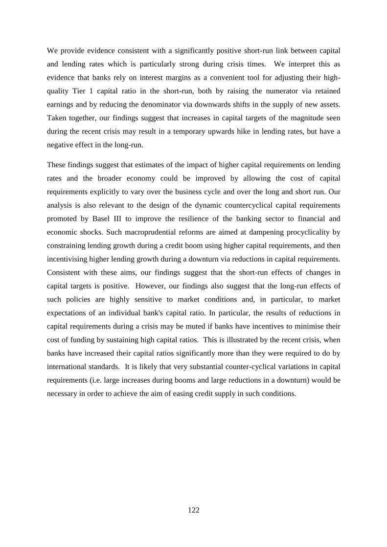
122
We provide evidence consistent with a significantly positive short-run link between capital
and lending rates which is particularly strong during crisis times. We interpret this as
evidence that banks rely on interest margins as a convenient tool for adjusting their high-
quality Tier 1 capital ratio in the short-run, both by raising the numerator via retained
earnings and by reducing the denominator via downwards shifts in the supply of new assets.
Taken together, our findings suggest that increases in capital targets of the magnitude seen
during the recent crisis may result in a temporary upwards hike in lending rates, but have a
negative effect in the long-run.
These findings suggest that estimates of the impact of higher capital requirements on lending
rates and the broader economy could be improved by allowing the cost of capital
requirements explicitly to vary over the business cycle and over the long and short run. Our
analysis is also relevant to the design of the dynamic countercyclical capital requirements
promoted by Basel III to improve the resilience of the banking sector to financial and
economic shocks. Such macroprudential reforms are aimed at dampening procyclicality by
constraining lending growth during a credit boom using higher capital requirements, and then
incentivising higher lending growth during a downturn via reductions in capital requirements.
Consistent with these aims, our findings suggest that the short-run effects of changes in
capital targets is positive. However, our findings also suggest that the long-run effects of
such policies are highly sensitive to market conditions and, in particular, to market
expectations of an individual bank's capital ratio. In particular, the results of reductions in
capital requirements during a crisis may be muted if banks have incentives to minimise their
cost of funding by sustaining high capital ratios. This is illustrated by the recent crisis, when
banks have increased their capital ratios significantly more than they were required to do by
international standards. It is likely that very substantial counter-cyclical variations in capital
requirements (i.e. large increases during booms and large reductions in a downturn) would be
necessary in order to achieve the aim of easing credit supply in such conditions.

123
This page is intentionally left blank.

124
Chapter 5 : Capital and profitability in banking: Evidence from
US banks
5.1 Introduction
In previous chapters, we have addressed banks‘ choice of capital ratio, how this affects the
growth of components of the balance sheet such as loans, risk-weighted assets and capital,
and the role of capital in determining banks‘ loan interest rates. These issues have been
analysed empirically using a unique regulatory dataset of UK banks. In this chapter of the
thesis, we present more preliminary work which seeks to apply a similar framework to the US
banking sector. In particular, we address the questions of whether there are asymmetries in
the relationship between capital and profitability of US banks which can be ascribed to
deviations from banks‘ own target capital ratios, and whether the relationship between capital
and profitability varies over financial cycles, extending the idea of ―In good times and bad‖
from Chapter 4. We use profitability as the measure of bank performance since it is a
commonly used proxy, is readily available for the banks in the sample and, unlike market
value, it does not require assumptions about the market value of debt. We carry out our
analysis using an exceptionally large dataset based on the US Federal Reserve Reports of
Condition and Income (―Call Reports‖), consisting of up to 15,000 banks over 30 years, in
total more than 1.6 million bank-quarter observations.
The specific empirical contributions of this chapter are as follows:
First, it is the first study to chart in a systematic way the changing relationship
between capital and profitability over such a long period of US banking history,
including the recent banking crisis as well as the savings and loan crisis of the late
1980s, employing sophisticated recent econometric techniques for dynamic panel
data.
The study embeds a model of banks‘ long-run target capital ratios 𝑘∗ which
recognises substantial heterogeneity over time and across different classes of banks in
terms of size and portfolio risk, allowing the relationship between the capital ratio and
proftiabiilty to vary depending on whether banks are above or below 𝑘∗. This is more
accurate that previous studies to have allowed non-linearity in the relationship since
125
they tend to divide banks into low and high capital without taking into account banks‘
internal capital targets (Osterberg and Thomson, 1996; Gropp and Heider, 2010).
The empirical analysis is in two parts. First, we extend the results of Berger (1995), a
seminal paper which developed the idea that the relationship between capital and profitability
may become positive during banking sector distress, namely the ―savings and loan crisis‖ of
the 1980s. This is ascribed to the ―expected bankruptcy costs‖ hypothesis, an important
component of the standard ―trade-off‖ theory, which states that in stressed conditions higher
capital reduces the required rate of return on risky debt by reducing the probability of default.
We apply more recent econometric techniques to estimate the Berger (1995) model more
robustly, and also extend the sample period up to 2010 to include the recent financial crisis.
We confirm that the original findings of Berger (1995) are robust to new techniques and
apply also, though to a lesser extent, in the recent financial crisis, since the negative
relationship between capital and profitability reduces significantly during this period.
However, there are a number of shortcomings with this model, which primarily concern the
use of a reduced form specification to capture structural relationships. While the findings are
attributed to the ―expected bankruptcy costs‖ hypothesis, this is difficult to distinguish from
other factors driving the long-run co-movement of capital and profitability. For example, a
more profitable bank may choose to hold a lower capital buffer since it expects to be able to
rely on internal funds to meet regulatory or market demands. Although this would usually
drive a negative rather than a positive relationship, it is also possible that under stressed
conditions, low profitability may lead a bank to increase leverage in order to rebuild
profitability (Milne and Whalley, 2002).
Consequently, in the second part of the analysis we present initial results from an improved
specification that attempts to address this problem and provide a more robust test of the
―expected bankruptcy costs‖ hypothesis. We estimate long run target capital ratios for US
banks, following a similar dynamic specification to that used in Chapter 3 and Chapter 4, and
include these in an extended version of Berger (1995) in order to remove the effects of the
long-run co-movement of capital and profits. Using the estimated target capital ratios as a
proxy for banks‘ own internal optimal capital ratios, we assess the hypothesis that there are
asymmetric effects of deviations from the optimal capital ratio. If a bank is below its optimal
capital ratio, then we expect deviations (deficits) to be positively correlated with capital since
banks can improve profitability by increasing capital, for example because investors are
concerned about expected bankruptcy costs. If a bank is above its optimal capital ratio, then
126
we expect deviations (surpluses) to be positively (negatively) correlated with capital since
banks can improve profitability by reducing increasing capital, consistent with the trade off
theory. Since we remove the effects of the long-run co-movement of capital and
profitability (via the inclusion of the target capital ratio itself in the regressions) our method
is a more robust test of the trade-off theory than the model based on Berger (1995).
The theoretical background is briefly as follows. Higher capital is often supposed to be
costly for banks due to capital market imperfections and tax advantages of debt, but
according to the popular ―trade-off‖ view higher capital may also reduce risk and hence lower
the premium demanded to compensate investors for the costs of bankruptcy. Therefore, there
may be a positive or negative relationship between capital and firm value in the short run
depending on whether a bank is above or below its optimal capital ratio. Indeed if banks are
successful in attaining their optimal capital ratios there may in fact be no short-run
relationship at all, since standard first order conditions imply that any change in capital has
no impact on value. In the long run, regulatory capital requirements may exceed the bank‘s
optimal capital ratio and drive a negative relationship between capital and value, if they are
binding. This implies that higher capital only reduces value if banks are above their optimal
capital ratios, for example due to capital requirements or unexpected shocks.
One implication of this is that banks‘ optimal capital ratios will rise during periods of
banking sector distress (―bad times‖), since in such conditions the expected costs of
bankruptcy rise. Since capital market imperfections mean that banks cannot immediately
adjust to the new optima, actual capital ratios tend to lag behind target capital ratios.
Consequently, we expect that the average relationship between capital and value across banks
will be cyclical, since in a stressed environment banks tend to be below their optimal capital
ratios, whereas during normal conditions (―good times‖), banks may either meet their optimal
capital ratios, in which case the relationship would be approximately zero, or overshoot, in
which case banks can increase value by reducing the capital ratio (e.g., taking advantage of
tax benefits of debt or implicit debt subsidies).
The long time period of our sample allows estimation of the relationship over several
financial cycles. First, in the 1980s and early 1990s the US banking sector was in a state of
upheaval due to the savings and loan crisis, which resulted in many bank failures and
occurred simultaneously with a widespread recession, though empirical studies differ as to
how far the recession was caused by banking problems (see reviews by Berger et al, 1995 and

127
Sharpe, 1995). Second, throughout the 1990s and early 2000s capital ratios rose and
profitability was consistently high. The higher capital ratios built up over this period have
been attributed to the higher capital requirements of Basel I and the Federal Deposit
Insurance Corporation Improvement Act (FDICIA) (Jackson et al 1999), increased market
discipline due to the removal of explicit and implicit state guarantees, and passive earnings
retention in a period of high profitability (Berger et al 2008; Flannery and Rangan, 2008).
Finally in the late 2000s came the global financial crisis (GFC) which resulted in substantial
losses and unprecedented levels of official support for the banking system.
In our study we use profitability as a measure of bank performance. Although this is an
imperfect measure of bank performance, it is a commonly used proxy in the banking
literature since it can be relatively easily calculated using accounting information and does
not require assumptions to be made about the market value of a firm‘s debt (see Mehran and
Thakor, 2011 for a good discussion of this problem related to banks and an attempt to deal
with it via the use of M&A data). Since the net income measure of profitability reflects
interest paid on debt it is also sufficient to test our hypothesis of interest that expected
bankruptcy costs drive a relationship between capital and value via the cost of funding. A
possible future extension would be to consolidate individual banks and identify them with
corresponding listed holding companies in order to test whether similar findings are observed
also for market returns as for profitability.
A significant challenge in identifying the causal link from capital to profitability is that the
direction of causality can plausibly run the other way. In the short run, high profitability may
drive higher capital ratios since profits are a source of capital. According to the pecking
order theory, internal funds are the least information-intensive source of funds and hence a
more profitable firm may retain earnings to fund known investment opportunities (Myers and
Majluf, 1984). Hence, the bank‘s capital is the sum of past profits less distributions. In the
long run, a more profitable bank may desire a smaller capital buffer since it knows that it will
be able to draw on internal funds to fund expected investment opportunities (Myers, 1984) or
avoid regulatory censure (Milne and Whalley, 2002). High profitability may also affect the
value of the tax deductability advantage offered by debt, since a firm that is not earning
profits does not pay tax on payments to equity holders (Modigliani and Miller, 1958; Miller,
1977). These two factors indicate that more profitable banks will choose to hold lower
capital ratios in the long run, i.e. a negative association. Milne and Whalley (2002) also point
out that a bank that is distressed may exhibit a positive association since low profits elicit a

128
gamble for resurrection involving higher portfolio risk and higher leverage. Alternatively,
high profitability may lead managers to retain excess profits in order to fulfil their own
personal projects or ambitions (Jensen, 1986). High profits may also increase the bank‘s
perceived charter value, providing incentive to hold higher capital ratios (Marcus, 1984;
Keeley, 1990). These factors predict positive causality from profits to capital in the long run.
We exploit the large cross section dimension of our dataset in order to distinguish the effects
of capital on profitability. We first estimate a long-run target capital ratio using a dynamic
partial adjustment model (PAM) specification. The large cross-section dimension of our
dataset is important since different banks will have very different target capital ratios in the
long run; for example, Berger and Bouwman (2012) show that the extent to which higher
capital ratios increase the performance of banks during stress episodes depends significantly
on bank size. Consequently, we estimate target capital ratios separately for nine different
groups defined in terms of their size and level of portfolio risk. In the next stage of our
analysis, we again exploit the cross-section of our dataset by including deviations from the
target capital ratio in a model of the return on assets (ROA), also controlling for the level of
the target capital ratio itself.
We find that in terms of the simpler model based on Berger (1995), the link from capital to
profitability is strongly cyclical, since it is strongly positive during the 1980s crisis, negative
throughout the 1990s and early 2000s, and then becomes positive again in the recent financial
crisis (though not to the same extent as during the 1980s crisis). The findings using the
improved model based on target capitalization shed further light on these trends. Our results
for the 1980s support the ―expected bankruptcy costs‖ hypothesis proposed by Berger (1995)
since we find a positive relationship for higher risk banks which are below their long-run
target capital ratios. However, the same is not true for the recent financial crisis in 2007-
2010 since there is no evidence for this period that low capital banks could improve
profitability by increasing capital ratios. This may reflect the role of official support in
softening the effect of market discipline.
Our results also shed light on the driving forces behind the increases in capitalization in the
1990s. From the basic model we learn that the relationship was strongly negative for most
banks, and our improved model shows that this was true for low risk and high risk banks.
Furthermore, there is only weak evidence of low capital banks being able to improve their
ROA by increasing capital in this period. These findings are not consistent with an increased

129
role for market discipline, as proposed, for example, by Flannery and Rangan (2008), since
that would suggest that low capital and high risk banks could increase profits by raising their
capital ratios. Our results suggest that banks were on average well above their optimal capital
ratios, and indeed they were also mostly well above the regulatory minimum capital
requirement in this period (Berger et al, 2008). This may indicate that high profitability drive
higher capital ratios during this period rather than the other way around.
We also use our results to draw policy implications. Our findings are relevant for a bank
regulator seeking to calibrate capital requirements, and the short-run effects of capital on
profitability are especially relevant for the design of so-called ―macroprudential‖ tools such
as counter-cyclical capital requirements.77
Such tools are designed to dampen credit cycles
by increasing the cost of new loans in a boom and stimulating lending during busts. Of
course, since counter-cyclical capital requirements did not exist during the sample period, it
is not possible to draw direct inferences about their effects from the historical data, and the
indirect inferences we do draw may not apply to the same extent in a regime with much
higher capital requirements that are binding on most banks (a regime that Basel III may
deliver). The extent to which the relationship co-moves with financial cycles provides
valuable information about the likely effects of counter-cyclical capital requirements, since to
be effective, banks must have incentives to change their capital ratios and lending policies in
response to cyclical adjustments in capital requirements. Our results indicate that banks‘ own
optimal capital ratios are cyclical, and since banks can increase their profitability by
increasing their capital ratios during periods of financial distress such as the 1980s or late
2000s, it is not likely that they would respond to reductions in capital requirements in such
conditions. During the late 2000s crisis the effects of market discipline were not as apparent
as during the 1980s crisis. During the 1990s, capital ratios were rising anyway so it seems
unlikely that increasing capital requirements in line with macroprudential aims would have
affected banks‘ capital choices. There were substantial downward pressures on banks‘
capital ratios in this period, but only for banks with high capital relative to their long-run
target capital ratios, which are the banks least likely to be affected by capital requirements.
This paper is structured as follows. In section 5.2 we review relevant literature on the
theoretical relationship between capital and profitability, and also review of trends in capital
and profitability in the US banking sector between 1976 and 2010. In section 5.3 we set out
77
For fuller reviews of macroprudential policy see Milne (2009) and Bank of England (2011).

130
the first part of our analysis, an extension of Berger (1995). In section 5.4 we set out the
second part of our analysis in which we present initial results of an improved model designed
to more robustly test our hypotheses. Section 5.4.3 concludes.
5.2 Literature review
5.2.1 Theory and evidence on the relation between capital and profitability in
banks
According to the second proposition of Modigliani and Miller (1958), investors‘ required
return on market equity is a negative linear function of the ratio of equity to debt, since higher
leverage raises the return demanded by shareholders. Most academic studies have argued
that deviations from the M-M theorems are particularly relevant for banks, and therefore
banks have an optimal capital ratio which maximises their value (Buser, Chen and Kane,
1981; Berger et al, 1995). At the core of this literature is the theory that the tax advantages of
debt and the advantages of government guarantees of debt ―trade off‖ against the expected
bankruptcy costs associated with low equity.
The effects of market discipline constrain banks to limit their leverage given that investors
are sensitive to the default risk of the bank, implying that banks with a high probability of
distress may be punished with a relatively high cost of uninsured funding (Nier and
Baumann, 2006; Flannery and Rangan, 2008; Berger, 1995; Flannery and Sorescu, 1996;
Covitz et al, 2004; Jagtiani et al, 2002; Morgan and Stiroh, 2001, Flannery, 1998; Sironi,
2003; and Gropp et al, 2002). Flannery and Rangan (2008) point out that the effect of market
discipline is muted by government guarantees, and therefore may be primarily observed in
periods where government guarantees are perceived to have been withdrawn, such as in the
early 1990s in the US when the FDICIA limited protection of uninsured bank creditors from
default losses and the Omnibus Budget Reconciliation Act of 1993 subordinated non-deposit
claims to a failed bank‘s deposits. A result which is at odds with this hypothesis is that of
Covitz et al (2004) which contends that the lack of observed significant market discipline
effects before this are the result of sample selection bias, since issuance is partly a function of
the potential spread, and after correcting for this bias they find a significant effect of default
131
risk on subordinated loan spreads throughout the period 1985-2002. It therefore seems likely
that higher portfolio risk increases the optimal capital ratio of a bank, especially when the
bank is subject to a greater degree of market discipline. An upwards shift in portfolio risk
results in a more negative relationship between capital and profitability in the short-run, until
the bank adjusts to its new optimal capital ratio.
The positive effect on capital ratios of market discipline from liability holders may be
reinforced by the incentives of the bank‘s owners and/or managers who also stand to lose
from the failure of the bank given that they will then lose future rents from the bank. The
charter or franchise value of a bank is the net present value of future rents which accrue to the
owners or managers, such as larger interest margins arising from market power or established
relationships, and provide incentives for banks to limit banks‘ risk taking at the expense of
liability holders (Bhattacharya, 1982; Marcus, 1984; Keeley, 1990; Rochet, 1992; Demsetz et
al, 1996; Hellmann et al, 2000). Hence, higher profitability creates incentives for banks to
limit risk-taking, including holding higher capital ratios as well as reducing portfolio risk.
One implication of this that has been explored by a number of recent studies is that higher
capital may help overcome agency problems arising from information asymmetries in the
bank-investor and bank-borrower relationships (Holmstrom and Tirole, 1997; Mehran and
Thakor, 2011; Allen Carletti and Marquez, 2011). A bank with a higher capital ratio has more
chance of surviving in the future and therefore has a greater incentive to monitor borrowers,
and investors take this into account when valuing claims on the bank. Allen, Carletti and
Marquez (2011) argue that this may result in large voluntary capital buffers in competitive
markets, since then higher capital is a more effective guarantee of the bank‘s monitoring
incentives and therefore allows the bank to offer more surplus to borrowers. The effect is to
increase banks‘ optimal capital ratios.
In the opposite direction, the effect of explicit or implicit government guarantees of banks‘
liabilities tend to reduce optimal bank capital. In particular, deposit insurance schemes
weaken the disciplining effect of depositors‘ required rate of return (Merton, 1978).
Perceptions amongst investors that the government will guarantee liabilities upon default
achieves a similar effect for uninsured debt (O‘Hara and Shaw, 1990; Nier and Baumann,
2006; Flannery and Rangan, 2008). The effect of a greater perceived likelihood of a safety
net being in place is to reduce optimal bank capital ratios.
132
Another plausible determinant of the optimal capital ratio is the relative information costs
associated with different sources of funding. According to the pecking order theory of
financing, raising equity or debt is costly for the bank because it conveys via a signal to the
market the owners‘ or managers‘ view of the prospects of the bank (Myers and Majluf,
1984). In the pecking order theory a firm‘s capital ratio is determined by the availability of
internally-generated funds from the past and the firm‘s investment opportunities. This may
generate an optimal capital ratio since the firm may also be concerned with maintaining
financial slack in order to be able to take advantage of future investment opportunities
(Myers, 1984). A highly profitable bank may therefore maintain a lower capital ratio since it
expects to be able to fund future investment out of earnings.
Banks‘ choices of capital ratio may also depend on their business plans. A bank with an
aggressive business strategy aimed at gaining market share may leverage up rapidly and
hence has a lower capital ratio. A bank that plans to acquire another bank may have an
incentive to maintain a higher capital ratio, for example so that it can satisfy regulators that
the resulting entity will be adequately capitalised (Berger et al, 2008). A bank that is
increasing its market share may hold a lower capital ratio consistent with a higher risk
strategy or simply because loan growth runs ahead of the ability to raise or retain capital
(Goddard et al, 2004).
A further important determinant of banks‘ capital ratios is regulation, in the form of explicit
minimum capital requirements and other supervisory pressures related to capital or
profitability. Such regulation is equivalent to an additional cost that is decreasing in the level
of capital that the bank holds. For banks that fall below the required minimum level of
capital it could include suspension of permissions, replacement of management or the
imposition of tough plans to restore capital adequacy, implying a positive probability that the
bank is closed so that its owners lose valuable franchise value (Merton 1978; Bhattacharya et
al 2002). Hence, several studies have analysed a trade-off between the benefits of holding
lower capital ratios and the expected costs of regulatory intervention, predicting that banks
optimally hold a buffer of capital over regulatory capital requirements (Estrella, 2004; Milne
and Whalley, 2002; Peura and Keppo, 2006; Barrios and Blanco, 2003; Repullo and Suarez,
2008; Heid, 2007). Following the same logic, the optimal capital buffer is likely to increase in
the degree of portfolio risk, though identifying this effect is made difficult by the fact that
risk averse banks may have higher capital and lower portfolio risk, and in the short run banks
with low capital buffers may ―gamble for resurrection‖ with higher risk (Lindquist 2003;
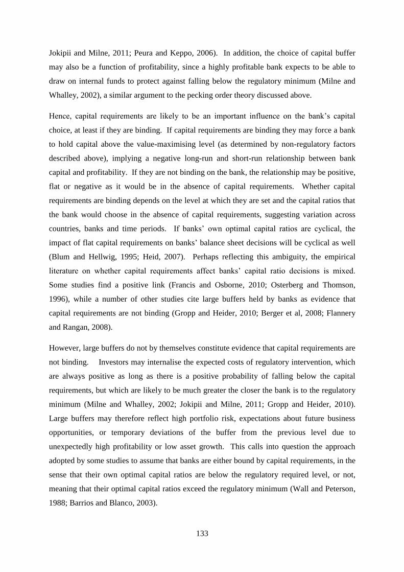
133
Jokipii and Milne, 2011; Peura and Keppo, 2006). In addition, the choice of capital buffer
may also be a function of profitability, since a highly profitable bank expects to be able to
draw on internal funds to protect against falling below the regulatory minimum (Milne and
Whalley, 2002), a similar argument to the pecking order theory discussed above.
Hence, capital requirements are likely to be an important influence on the bank‘s capital
choice, at least if they are binding. If capital requirements are binding they may force a bank
to hold capital above the value-maximising level (as determined by non-regulatory factors
described above), implying a negative long-run and short-run relationship between bank
capital and profitability. If they are not binding on the bank, the relationship may be positive,
flat or negative as it would be in the absence of capital requirements. Whether capital
requirements are binding depends on the level at which they are set and the capital ratios that
the bank would choose in the absence of capital requirements, suggesting variation across
countries, banks and time periods. If banks‘ own optimal capital ratios are cyclical, the
impact of flat capital requirements on banks‘ balance sheet decisions will be cyclical as well
(Blum and Hellwig, 1995; Heid, 2007). Perhaps reflecting this ambiguity, the empirical
literature on whether capital requirements affect banks‘ capital ratio decisions is mixed.
Some studies find a positive link (Francis and Osborne, 2010; Osterberg and Thomson,
1996), while a number of other studies cite large buffers held by banks as evidence that
capital requirements are not binding (Gropp and Heider, 2010; Berger et al, 2008; Flannery
and Rangan, 2008).
However, large buffers do not by themselves constitute evidence that capital requirements are
not binding. Investors may internalise the expected costs of regulatory intervention, which
are always positive as long as there is a positive probability of falling below the capital
requirements, but which are likely to be much greater the closer the bank is to the regulatory
minimum (Milne and Whalley, 2002; Jokipii and Milne, 2011; Gropp and Heider, 2010).
Large buffers may therefore reflect high portfolio risk, expectations about future business
opportunities, or temporary deviations of the buffer from the previous level due to
unexpectedly high profitability or low asset growth. This calls into question the approach
adopted by some studies to assume that banks are either bound by capital requirements, in the
sense that their own optimal capital ratios are below the regulatory required level, or not,
meaning that their optimal capital ratios exceed the regulatory minimum (Wall and Peterson,
1988; Barrios and Blanco, 2003).

134
In addition, capital requirements may affect the market‘s view of the level of capital for a
bank. Assuming that supervisory assessments and related pressures on capital are to some
extent publicly available and represent more information than is available to the market
(Deyoung et al, 2001; Berger et al, 2000), capital requirements may also alter investors‘
perception of the capital ratio that is necessary to assure the solvency of the bank, even for a
bank that has a sizeable buffer of capital. Hence, the effects of market discipline are closely
interrelated with capital requirements (e.g., see Jackson et al, 1999; Osterberg and Thomson,
1996). Since investors penalise a bank with insufficient capital with a higher required rate of
return, the effect of capital requirements is that banks with capital ratios close to the
regulatory minimum are likely to have a more positive relationship between capital and
profitability than those that are less constrained, other things equal.
The discussion above offers a number of competing drivers of banks‘ capital ratios which
suggest that the relationship could be positive or negative depending on banks‘
circumstances. Most empirical studies that have examined the relationship between capital
and profitability have found a positive relationship, across a variety of different markets and
time periods (Angbazo, 1997; Demirguc-Kunt and Huizinga, 1999; Vennet, 2002; Nier and
Baumann, 2006; Flannery and Rangan, 2008). This could be attributed to the pecking order
theory since high earnings in the past drive higher capital in the present, although, as noted
above, both the buffer capital and pecking order perspectives predict that in the long run
higher profitability leads to a lower desired capital ratio. Morgan and Stiroh (2001) look
directly at the relationship between capital ratio and spreads paid on debt and find a
relationship that is positive but weak.
However, the studies cited above have a limitation since they impose the restriction that the
relation between capital and profitability is linear and homogeneous across banks and time
periods. The positive relationship found is therefore an average relationship across banks and
time periods. We are aware of three studies that have tried to relax this constraint. Berger
(1995) estimates a linear relationship between ROE and lagged capital for US commercial
banks but allow the relationship (and in fact the whole model) to vary between the periods
1983-89, in which banks in general are argued to have been below their optimal capital ratios,
and 1990-92 in which they are believed to have been above their optimal capital ratios. The
coefficient is positive in the first period and negative in the second, consistent with the theory
above that optimal capital ratios rise during periods of distress and banks depart from their
optimal capital ratios in the short run. However, this method does not allow the relationship

135
to vary across banks, which from a theoretical point of view it is likely to do depending on
whether banks are above or below their optimal capital ratio and how close they are to it.
Osterberg and Thomson (1996) explore the determinants of leverage in US banking holding
companies (BHCs) in the period 1987-8. Their specification includes a linear earnings term
and an interaction term consisting of earnings multiplied by the buffer over capital
requirements. They find that the capital ratio and earnings are positively correlated, and this
relationship is more positive for banks which are close to the regulatory minimum. Gropp
and Heider (2010) study the determinants of leverage for large US and European banks over
the period 1991-2004. They include return on assets and also the return on assets multiplied
by a dummy variable which is equal to 1 if the bank is close to its regulatory requirement.
The ROA and capital ratio are negatively related, but when capital is close to the regulatory
minimum, the overall relationship is insignificantly different from zero.
The non-linear specifications used in Gropp and Heider (2010) and Osterberg and Thomson
(1996) suffer from a drawback since the relationship can only vary for banks with low
capital. The factors driving the relationship between capital and profitability identified above
point to a relationship that could differ depending on whether a bank is above or below the
optimal capital ratio and therefore the relationship could vary between high capital and
medium capital banks as well as for low capital banks. A related issue is that the studies
attribute the non-linearity close to the regulatory minimum to the effects of regulation. While
it is true that regulation may drive a particularly strong positive relationship close to the
regulatory minimum, market discipline could drive similar effects and it is questionable
whether those studies have truly identified an incremental regulatory effect distinct from the
trade-off factors which are relevant for any firm.
In section 5.3, we set out a specification for the relationship between capital and profitability
which allows for heterogeneity across time and interaction with the level of capital across
banks. We apply this specification to an updated dataset including commercial banks through
the recent financial crisis.
5.2.2 Trends in capital and profitability of US banking sector, 1976-201078
78
We do not attempt a full review of trends in the US banking industry here, preferring to identify only those
facts that are most salient to our analysis. For a more complete review see DeYoung (2010).
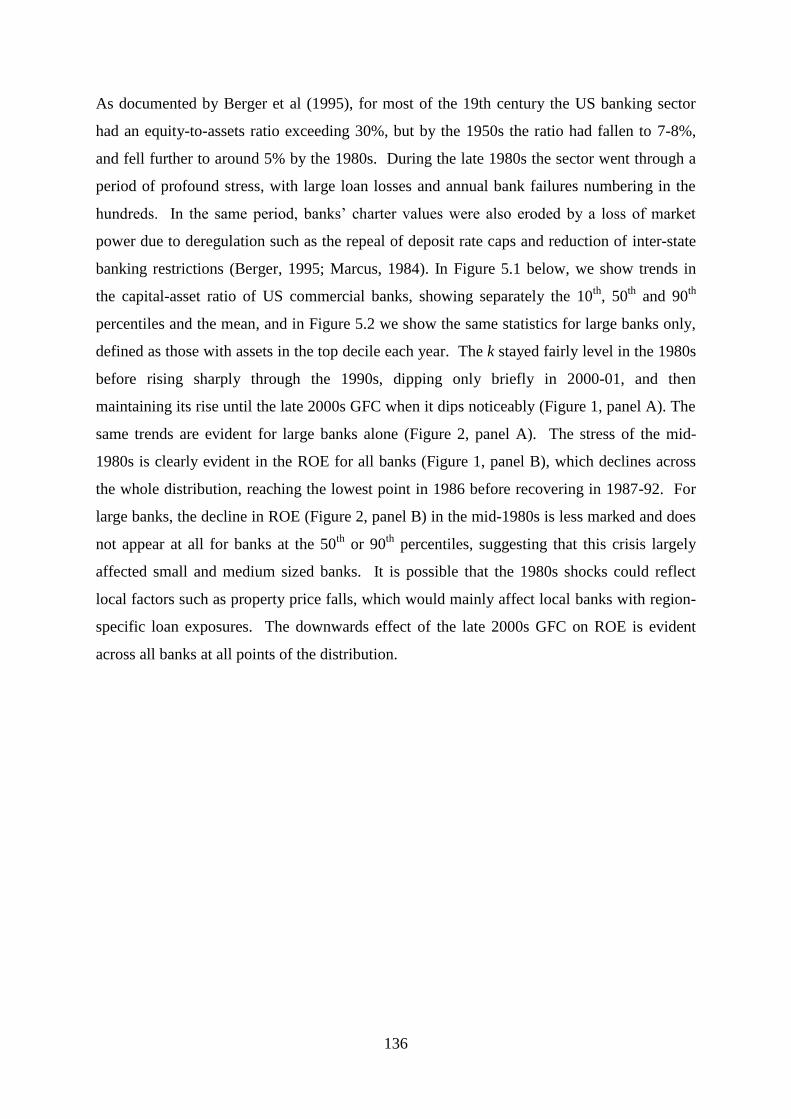
136
As documented by Berger et al (1995), for most of the 19th century the US banking sector
had an equity-to-assets ratio exceeding 30%, but by the 1950s the ratio had fallen to 7-8%,
and fell further to around 5% by the 1980s. During the late 1980s the sector went through a
period of profound stress, with large loan losses and annual bank failures numbering in the
hundreds. In the same period, banks‘ charter values were also eroded by a loss of market
power due to deregulation such as the repeal of deposit rate caps and reduction of inter-state
banking restrictions (Berger, 1995; Marcus, 1984). In Figure 5.1 below, we show trends in
the capital-asset ratio of US commercial banks, showing separately the 10th
, 50th
and 90th
percentiles and the mean, and in Figure 5.2 we show the same statistics for large banks only,
defined as those with assets in the top decile each year. The k stayed fairly level in the 1980s
before rising sharply through the 1990s, dipping only briefly in 2000-01, and then
maintaining its rise until the late 2000s GFC when it dips noticeably (Figure 1, panel A). The
same trends are evident for large banks alone (Figure 2, panel A). The stress of the mid-
1980s is clearly evident in the ROE for all banks (Figure 1, panel B), which declines across
the whole distribution, reaching the lowest point in 1986 before recovering in 1987-92. For
large banks, the decline in ROE (Figure 2, panel B) in the mid-1980s is less marked and does
not appear at all for banks at the 50th
or 90th
percentiles, suggesting that this crisis largely
affected small and medium sized banks. It is possible that the 1980s shocks could reflect
local factors such as property price falls, which would mainly affect local banks with region-
specific loan exposures. The downwards effect of the late 2000s GFC on ROE is evident
across all banks at all points of the distribution.
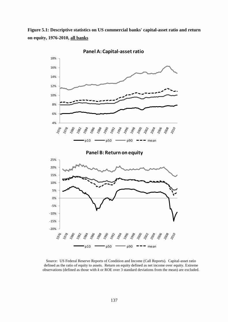
137
Figure 5.1: Descriptive statistics on US commercial banks' capital-asset ratio and return
on equity, 1976-2010, all banks
Source: US Federal Reserve Reports of Condition and Income (Call Reports). Capital-asset ratio
defined as the ratio of equity to assets. Return on equity defined as net income over equity. Extreme
observations (defined as those with k or ROE over 3 standard deviations from the mean) are excluded.
4%
6%
8%
10%
12%
14%
16%
18%
Panel A: Capital-asset ratio
p10 p50 p90 mean
-20%
-15%
-10%
-5%
0%
5%
10%
15%
20%
25%
Panel B: Return on equity
p10 p50 p90 mean
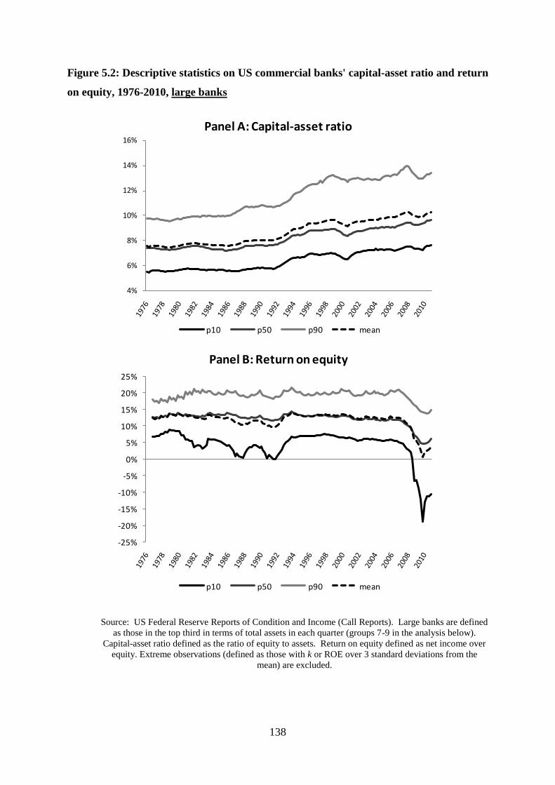
138
Figure 5.2: Descriptive statistics on US commercial banks' capital-asset ratio and return
on equity, 1976-2010, large banks
Source: US Federal Reserve Reports of Condition and Income (Call Reports). Large banks are defined
as those in the top third in terms of total assets in each quarter (groups 7-9 in the analysis below).
Capital-asset ratio defined as the ratio of equity to assets. Return on equity defined as net income over
equity. Extreme observations (defined as those with k or ROE over 3 standard deviations from the
mean) are excluded.
4%
6%
8%
10%
12%
14%
16%
Panel A: Capital-asset ratio
p10 p50 p90 mean
-25%
-20%
-15%
-10%
-5%
0%
5%
10%
15%
20%
25%
Panel B: Return on equity
p10 p50 p90 mean

139
Partly as a result of the experience of the 1980s, the period from 1989-93 saw a considerable
tightening of regulatory standards. These measures had been foreshadowed by the
introduction of a leverage ratio requirement in 1984, which required ‗primary‘ capital (equity
plus loan loss reserves) to be more than 5.5% of assets and the total of ‗primary‘ capital and
‗secondary‘ capital (primarily qualifying subordinated debentures) to be over 6% of assets,
which seems to have been effective in raising banks‘ capital ratios (Wall and Peterson 1988).
The forthcoming risk based capital requirements had also been flagged in the publication of a
joint US/UK proposal on risk-based capital (RBC) requirements in 1986 (Osterberg and
Thomson 1996). The increase in capital-asset ratios of large banks in 1985-89 evident in
Figure 5.1 may reflect these measures, though there is no similar trend for small banks.
Risk-based capital requirements were formalised in the international Basel Accord of 1988,
and then introduced in the US between 1990 and 1992, and a higher leverage ratio
requirement was also introduced in 1990 (Berger et al, 1995). The leverage ratio may have
been the binding constraint for many banks whose portfolios contained mainly low risk-
weighted assets such as mortgages and government securities (Berger and Udell, 1994). At
the same time, the FDICIA introduce prompt corrective action which increased supervisory
sanctions for breaching regulatory minimum capital ratios, and also introduced risk-based
deposit insurance premia. The combination of these regulatory measures incentivised banks
to raise their capital ratios (Berger et al, 1995) and we can clearly see the effects of this in
Figure 5.1 and Figure 5.2 which show a substantial increase in capital ratios in the early
1990s for large and small banks, and across the whole distribution.
The new regulatory standards were accompanied by a sharp increase in the capitalization of
US banks and a credit crisis and a recession across much of the US, suggesting that
adjustment to higher standards induced deleveraging and a contraction in banks‘ supply of
credit to the real economy, exacerbated by the relatively high risk weights given to corporate
lending compared to government debt (Berger et al, 1995). However, the large literature on
this subject provides rather mixed conclusions, since there is not a consistent association
between closeness to the regulatory minima and changes in lending patterns at individual
banks (e.g. see reviews in Berger et al, 1995; Sharpe, 1995; Jackson et al, 1999). This
suggests that while regulatory changes may have played a role, much of the decline in credit
can be attributed to a recession-induced contraction in demand.
140
A notable feature of Figure 5.1 and Figure 5.2 is that capital ratios kept increasing throughout
the 1990s and into the early 2000s, for both large and small banks. While this does not rule
out that the regulatory standards of the early 1990s were partly responsible for the increase, it
does suggest that other factors were at play, since by the early 2000s capital ratios reached
levels far in excess of the regulatory minima (Berger et al, 2008; Flannery and Rangan,
2008). One explanation for this trend is enhanced market discipline. In the 1980s, bank
creditors enjoyed substantial guarantees effectively making large banks ―too big to fail‖, but a
number of regulatory changes were made in the 1980s and 1990s which had the effect of
reducing uninsured liability holders‘ perceptions of the likelihood that they would be rescued
upon default of a bank, including purchase and assumption transactions, prompt corrective
action, least cost resolution and depositor priority (Covitz et al, 2004; Flannery and Rangan,
2008). Combined with much higher asset volatility over this period (driven in part by the
1997 Asian crisis and 1998 Russian default/LTCM problems), it has been argued that
increased market discipline raised banks‘ optimal capital ratios well in excess of capital
requirements (Flannery and Rangan, 2008). Berger et al (2008) also note that that banks‘
profitability rose in the early 1990s and remained at high levels into the mid-2000s, which is
also evident from our Figure 5.1 and Figure 5.2, and this may have contributed to higher
capital for reasons explained in section 5.2.1 above.
A number of other trends were evident in the 1990s onwards. The risk-weighted capital
ratios stipulated by the Basel Accord fell, even as the unweighted ratio continued to rise
(Berger et al, 2008). Part of the explanation for this phenomenon is the sector‘s adaption to
the imperfect risk-sensitivity in the rules. For example, a favourable treatment of
securitisation under Basel I may have contributed to the growth of banks‘ involvement and
the pervasive ―originate-to-distribute‖ business model in this period, although certain early
studies failed to find a direct link between capital adequacy and the decision to securitize
assets (Carlstrom and Samolyk, 1995; Jagtiani et al, 1995). Thirdly, this period saw
substantial consolidation in the banking sector, due in part to deregulation noted above,
particularly the removal on restrictions on interstate banking and on combining different
banking activities such as investment banking with traditional banking activity (Berger et al,
1999).
Last but certainly not least, our sample period ends with the global financial crisis of 2007-
09. The crisis was triggered by losses on subprime loans in the US which banks had tranched
and sold on to a diverse range of investors including other banks, causing a contagious loss of
141
confidence in the balance sheets of banks and a collapse in interbank lending (Brunnermeier,
2009). The underlying causes of the crisis probably included global macroeconomic
imbalances and low interest rates (see Merrouche and Nier, 2011 for a review of this
emerging literature) and continue to be debated (see Lo, 2012). There are several
implications for our consideration of capital and profitability. First, banks suffered
substantial losses due to bad credit and were also forced to pay much higher rates of return on
short-term and unsecured debt, contributing to much lower profitability over this period.
Second, the capital ratios of banks have been a key determinant of profitability and survival
during the crisis (Berger and Bouwman, 2012). As a result, the crisis has been associated
with regulatory demands for much higher capital ratios including in the Dodd-Frank Act and
international Basel III standards to which the US is a signatory. Significantly, the Basel III
package includes calls for a leverage ratio based on the ratio of capital to assets, which as
noted above had been a feature of US capital regulation since 1990.
The financial crisis of 2008-2010 has also seen unprecedented levels of official support for
the banking sector, including emergency liquidity support such as the Troubled Asset Relief
Program (TARP) which was launched in late 2008 to purchase assets from banks and later
directly purchased the equity of banks, and other programmes operated by the Federal
Reserve. Monetary policy was very loose by historical standards and fiscal policy was also
used to stimulate the economy. Perhaps as a result of these dramatic actions, the actual rate
of bank failure was much lower than the earlier savings and loan crisis in the late 1980s.
Figure 5.3 shows the number of annual bank failures or assistance transactions recorded in
each year from 1976 to 2010 by the Federal Deposit Insurance Corporation (FDIC) (dashed
line, left axis), and the assets of failed or assisted banks as a percentage of total banking
assets (full line, right axis). The number of failed banks reached 400-500 per year in the late
1980s, but in the recent GFC it peaked at only 150 per year. This may partly reflect the fact
that there were many fewer banks in the industry at the time of the GFC. It also reflects the
fact that failures were much more concentrated in relatively few large banks, which can be
seen from the fact that assets of failed banks peaked at about 16% of total banking assets in
200979
compared with only 5% in 1988.
79
The biggest bank that failed or received assistance from the FDIC in 2009 was Bank of America whose assets
are 11% of the total industry assets. The next biggest in that year are FIA Card Services, part of Bank of
America (1.2%) and Countrywide (0.9%).

142
Figure 5.3: FDIC bank failures 1976-2010
Notes: FDIC failed banks database was used to identify banks which failed or were assisted in each year. The
assets of failed banks from this database are expressed as a percentage of total banking assets calculated from
Federal Reserve Reports of Conditions and Income (call reports).
5.3 Extending the results of Berger (1995)
The first stage of our analysis is to extend the results of Berger (1995). As noted above, this
paper‘s important contribution was to identify that the effect of capital on the profitability of
banks is likely to be cyclical. During the period 1983-89, which was a period of significant
stress in the US banking sector (the ―savings and loan crisis‖), lagged values of the k are
found to be positively correlated with ROE, confirming a Granger causal relationship. It is
argued that, during this period, banks‘ optimal capital ratios rose substantially, and ―banks
that raised their capital toward their new, higher equilibria had better earnings than other
banks through lower interest rates paid on uninsured debt. This is because higher capital
reduces the probability that uninsured debt holders will have to bear the administrative, legal,
and asset devaluation costs of bank failure, and therefore lowers the required premium on
uninsured debt for banks that increase their capital ratios.‖ The same model is re-run during
the early period of 1990-92, by which time banks‘ capital ratios had increased substantially as
shown in Figure 5.1 above. A negative relationship is found for this period. Berger
concludes, ―The negative causality during this later period suggests that banks may have
0%
2%
4%
6%
8%
10%
12%
14%
16%
18%
0
100
200
300
400
500
600 Pe
rcen
tage o
f ban
king asse
tsN
um
be
r o
f b
anks
Number of failed/assisted banks
Failed/assisted bank assets as % of total assets
143
overshot their optimal capital ratios, as reduced risk lowered optimal capital ratios and
regulatory changes and higher earnings raised actual capital ratios‖.
Our first goal is to find out whether the original results of Berger (1995) stand up to more
modern econometric examination, and whether the estimated positive relationship in stressed
conditions also applies during the more recent period of banking distress. More specifically,
we extend the results of Berger (1995) in several ways.
We extend the sample period to the recent financial crisis, estimating the model on
five-year rolling windows from 1977-1981 to 2006-2010.
We address the estimation problem of lagged dependent variable bias which is likely
to reflect the earlier estimates, using more recently developed econometric techniques
based on the general method of moments.
We introduce controls for the banks‘ portfolio risk, including the standard deviation
of ROE which we argue is a more general measure of risk than the measures used by
Berger (1995) and may better capture banks‘ off-balance sheet, investment banking
and trading activities.
5.3.1 Data and specification
The basic model used in Berger (1995) is summarised by Equation (5.1). ROE is regressed
on three lags of itself and of k, controlling for other potential determinants of profitability in
the vector 𝑋𝑖,𝑡−1 and bank and time effects. We estimate Equation (5.1) on a set of 30 5-year
rolling windows which we denote 𝜏, starting in 1977-1981 and ending in 2006-2010. Hence,
each set of coefficient estimates are specific to a window 𝜏.
𝑅𝑂𝐸𝑖𝑡 = 𝛼𝜏 + 𝑐𝑖𝜏 + 𝜃𝑡𝜏 + 𝛽𝑗𝜏1 𝑘𝑖 ,𝑡−𝑗
𝐽
𝑗=1
+ 𝛽𝑗𝜏2 𝑅𝑂𝐸𝑖,𝑡−𝑗
𝐽
𝑗=1
+ 𝜷𝝉′ 𝑿𝒊,𝒕−𝟏 + 𝜸𝝉
′ 𝑺𝑰𝒁𝑬𝒊𝒕 + 휀𝜏𝑖𝑡
(5.1)
This model deals with causality from ROE to k by including J lags of the two dependent
variables, which is equivalent to assuming that k is predetermined, i.e. that while 𝑅𝑂𝐸𝑖𝑡 may
144
affect 𝑘𝑖𝑡 , 𝑅𝑂𝐸𝑖𝑡 does not affect 𝑘𝑖 ,𝑡−1 since profitability would not affect past values of 𝑘.
We calculate the effect of lags of k and ROE on ROE by summing the coefficient over the J
lags, i.e. 𝛽1 = 𝛽𝑗1𝐽
𝑗=1 and 𝛽2 = 𝛽𝑗2𝐽
𝑗=1 .
The vector of control variables 𝑋𝑖𝑡 include variables which previous studies have found
helpful in explaining both capital and profitability. The coefficients on 𝐶𝐴𝑅 may then be
interpreted as the effect of deviations from the level of capital that would be expected given
the bank- and time-specific control variables, including bank and time effects (see Berger,
1995, p.440). Hence, the control variables are chosen to include both variables helpful in
explaining leverage and those found helpful in explaining ROE (there is likely to be
substantial overlap). We include bank- and time effects and also nine dummy variables
representing deciles of the distribution of total assets in each year (SIZE). We include
controls for the level of portfolio risk. These are expected to be positively correlated with
ROE since higher risk is linked to higher returns for shareholders. Portfolio risk is also
expected to be positively correlated with k since investors trade off capital and risk in order to
target a given probability of default (Jokipii and Milne, 2009). We include a set of different
measures of portfolio risk identified by previous studies (e.g. Osterberg and Thomson, 1996;
Jokipii and Milne, 2009; Berger, 1995), each capturing a separate aspect of risk:
Ratio of commercial loans to total assets. Commercial lending is generally
acknowledged as the highest risk type of loans and consequently was given a 100%
risk weight in the first Basel Accord. This is available for the whole sample period.
Ratio of net charge-offs to total assets. Charge-offs are a good ex-post measure of
risk since they indicate the level of losses the bank has experienced. We construct a
measure of annualised charge-offs and then, since charge-offs tend to be very volatile,
we calculate a moving average over three quarters. This is available for the whole
sample period.
Ratio of non-performing loans to total assets. Indicates the level of likely future
losses on loans. This is available from 1984 onwards.
Ratio of risk-weighted assets to total assets. Introduced by the Basel Accord in
1990, this variable serves as an ex-ante measure of a bank‘s risk. It has the advantage
145
that it captures the risk of trading book activities and off-balance sheet commitments.
This series starts in 1996 (before then it does not include trading book assets).80
Standard deviation of return on equity. From an investor‘s point of view a key
measure of the risk of a bank is the volatility in profitability (Flannery and Rangan,
2008). We calculate the standard deviation of the quarterly book return on equity
over the last three years.81
This has the advantages that it does not rely on any ex ante
weighting of different asset types (as do RW and C&I) and it captures volatility in
profits as well as level of losses (which are captured by CHARGE, NPL). It also
captures off-balance sheet and trading activities. This variable is available for the
whole sample period.
We also include proxies for the competitive position of a bank‘s markets, which is likely to
be a key determinant of profitability according to the structure-conduct-performance
framework (e.g., see Goddard et al, 2004). As described above, the US banking sector has
become much more concentrated over the period of our analysis, though the removal of
restrictions on interstate banking and technological advances may also have made the market
more competitive at a local level (Berger et al, 1999). Therefore, we also include measures
of market structure which are based on those used by Berger (1995) and Berger et al (1999).
In order to capture local market concentration, we first identify local banking markets as
Metropolitan Statistical Areas (MSAs) and non-MSA counties. The FDIC‘s annual Summary
of Deposits data gives details of each bank‘s deposits in each local market. We calculate the
bank‘s share of local market deposits (SHARE), the Herfindahl index for each market
(HERF), and the growth of deposits in each market-year combination (GROWTH). For each
bank, we calculate the weighted average of each of these variables over the local markets in
which it operates, with weights given by the share of its deposits in each market. We also
calculate the share of a bank‘s deposits in urban markets (i.e. MSAs).
Finally we also include the ratio of operating costs to total assets averaged over the last two
years (AC), as a proxy for operating efficiency. This variable is only available from 1984
onwards.
80
Note that Berger (1995) includes RWA going back all the way to 1982, based on proxy data for balance sheet
components. We were unable to obtain this data from public sources. 81
Our preference would be to use the return on market equity rather than book equity, but these are not available
for our dataset of commercial banks.
146
In order to be consistent with Berger (1995), we first estimate Equation (5.1) using fixed
effects. However, we note that this estimation strategy suffers from lagged dependent
variable (LDV) bias since the fixed effect is correlated with the LDV, ROEi,t−j3j=1 .
Therefore, we also adopt the system GMM method developed by Blundell and Bond (1998)
to estimate Equation (5.1). In this approach, the differenced LDV is instrumented with
lagged levels, and the lagged LDV in levels is instrumented using lagged first differences.
This estimator is available in one-step and two-step variants. While the two-step is
asymptotically more efficient, the standard errors are downward-biased and must be corrected
using the adjustment developed by Windmeijer (2005).82
We estimate both one-step and
two-step versions of Equation (5.1). The number of lags of k and ROE, J, is set at 3
consistent with Berger (1995).
The data are taken from the quarterly US Federal Reserve Reports of Condition and Income
(Call Reports). We drop failed banks in the year in which they fail (using an FDIC database
of bank failures) and banks under ―special analysis‖ such as bankers‘ banks, credit card
banks, depository trust companies, and bridge entities. When k falls below 1%, equity is
replaced with 1% of assets for calculation of other variables with equity in the denominator.
This avoids extreme and implausible values when equity is very low. Equity and assets are
calculated as the average of the current value and three (quarterly) lags.83
Finally, we drop
extreme observations of k and ROE, defined as those which are greater than three standard
deviations from the mean in each year. In total, our sample has just under 15,000 banks at
the beginning of the sample period in 1977, falling to under 11,000 by 1995 and around 7000
by 2010. Our estimations are based on annual data using the fourth quarter in each year, a
total of 30 time periods. The means of the control variables are shown in Table 5.1,
separately for selected 5-year windows.
82
All of this is accomplished using the very useful xtabond2 program developed in Stata by David Roodman
(2004). 83
These steps to clean the data are based on those noted in Berger (1995) and Berger et al (2004).
147
Table 5.1: Descriptive statistics for control variables, 1977-2010
1976-
1980
1981-
1985
1986-
1990
1991-
1995
1996-
2000
2001-
2005
2006-
2010
BANKSHARE 0.16 0.16 0.16 0.15 0.13 0.12 0.12
HERF 0.26 0.25 0.25 0.23 0.19 0.19 0.19
GROWTH 0.12 0.11 0.04 0.07 0.04 0.06 0.05
MSA 0.41 0.44 0.45 0.46 0.51 0.53 0.54
CHARGE 0.001 0.003 0.004 0.002 0.001 0.002 0.002
C&I 0.11 0.13 0.12 0.09 0.10 0.10 0.10
SDROE 0.02 0.04 0.06 0.04 0.02 0.02 0.03
NPL
0.01 0.01 0.01 0.01 0.01 0.01
RW 0.64 0.67 0.70
SIZE 0.50 0.51 0.51 0.50 0.51 0.51 0.51
Notes: Summary statistics for the standard deviation of ROE (SDROE), the ratio of commercial and industrial
loans to total assets (C&I), the ratio of charge offs to total assets (CHARGE), the ratio of non-performing loans
to total assets (NPL), the ratio of risk weighted assets to total assets (RW), the bank‘s share of local deposit
markets (BANKSHARE), the Herfindahl index of concentration in the bank‘s local markets (HERF), the share
of a bank‘s deposits in urban markets (MSA), the growth of local market deposits (GROWTH), the ratio of
operating costs to total assets (AC) and size index (SIZE).
5.3.2 Results
We show the results of our estimation of Equation (5.1) in Figure 5.4 below. Panel A shows
the fixed effects results, which are the most consistent with the method used by Berger
(1995). Panels B and C show the results using one-step and two-step GMM respectively.
Consistent with that paper‘s findings, the effect of k on ROE turns strongly positive in the
late 1980s, before turning negative in the early 1990s. These findings are consistent across
all three estimators, showing that the original Berger (1995) findings are robust to more
modern econometrics. After the Berger (1995) sample period, we show that the negative
relationship from k to ROE observed in the early 1990s persists throughout the 1990s. The
FE estimates show that the negative relationship continued through the late 1990s and into
the early 2000s, whereas the more robust GMM estimates show that the negative effect
reduced in magnitude and was close to zero by the late 1990s. In the late 2000s, with the

148
onset of the GFC, all three estimators show the relationship becoming markedly less
negative, though only the GMM estimators find that it is significantly positive. These
findings provide support for the idea that banks that increased capital ratios before and during
the GFC had higher ROE, other things equal (although we note various concerns with this
specification in section 5.3.3).
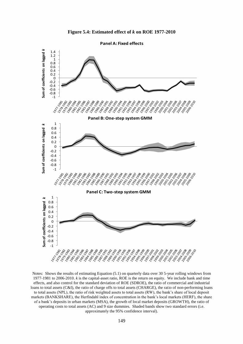
149
Figure 5.4: Estimated effect of k on ROE 1977-2010
Notes: Shows the results of estimating Equation (5.1) on quarterly data over 30 5-year rolling windows from
1977-1981 to 2006-2010. k is the capital-asset ratio, ROE is the return on equity. We include bank and time
effects, and also control for the standard deviation of ROE (SDROE), the ratio of commercial and industrial
loans to total assets (C&I), the ratio of charge offs to total assets (CHARGE), the ratio of non-performing loans
to total assets (NPL), the ratio of risk weighted assets to total assets (RW), the bank‘s share of local deposit
markets (BANKSHARE), the Herfindahl index of concentration in the bank‘s local markets (HERF), the share
of a bank‘s deposits in urban markets (MSA), the growth of local market deposits (GROWTH), the ratio of
operating costs to total assets (AC) and 9 size dummies. Shaded bands show two standard errors (i.e.
approximately the 95% confidence interval).
-1-0.8-0.6-0.4-0.2
00.20.40.60.8
11.21.4
Sum
of
coe
ffic
ien
ts o
n la
gge
d k
Panel A: Fixed effects
-1-0.8-0.6-0.4-0.2
00.20.40.60.8
1
Sum
of
coe
ffic
ien
ts o
n la
gge
d k
Panel B: One-step system GMM
-1
-0.8
-0.6
-0.4
-0.2
0
0.2
0.4
0.6
0.8
1
Sum
of
coe
ffic
ien
ts o
n la
gge
d k
Panel C: Two-step system GMM
150
5.3.3 Problems with the model based on Berger (1995)
While Berger (1995) is an important contribution in the sense of identifying the idea that
capital may have different effects on bank performance at different stages of the financial
cycle, there are a number of problems with the above model, which we discuss below. The
last two of these are partially addressed by robustness checks by Berger (1995).
Estimated relations are reduced form rather than structural
The first problem is that Equation (5.1) yields only reduced form estimates, making it
difficult to put an economic interpretation on the estimates. Interpreting 𝛽1 as the causal
effect of k on ROE requires the assumption that any association between lagged k and current
ROE reflects the effect of k on ROE. In econometric terms we treat k as predetermined,
which means that future values of ROE do not affect current values of k. This removes one
potential source of endogeneity in the short run, which is that profits provide a source of
capital. Assuming that a bank with ROE higher than expected may retain the additional
earnings as capital, higher ROE may result in higher k in the future. However, it is difficult
to see how higher ROE could affect past values of k via this particular mechanism, so
theoretically at least the equation is protected from this concern.
In the long run, it is possible that the level of profitability may affect a bank‘s optimal capital
ratio. For example, a more profitable bank may expect to have higher ROE in the future and
therefore chooses to hold a lower precautionary buffer, knowing it will be able to rely on
internal funds to ensure it meets the desired levels in future (Milne and Whalley, 2002).
Also, profitability plays an important role in the trade-off theory of capital structure, since the
tax deductibility of debt is only relevant for profitable banks which expect to be taxed on
their profits. Hence, highly profitable banks may tend to hold lower ks as a result. These
long-run effects are different from the short run effect of capital described above, but could
still be captured by controlling for lagged values of ROE which capture the bank‘s
expectation about its future ROE.
It is also possible that 𝛽1 could reflect a bank adopting an expansionary strategy in which it
seeks to increase its market share, by reducing margins in order to expand its loan book.
Since the bank has cut its margins it is likely that the bank will experience a decline in book
ROE, at least during the period of transition. However, k may also fall since the bank‘s assets
are increasing beyond its ability to retain or raise capital. This could plausibly drive
151
correlation between ROE and lagged k since the banks may raise debt in advance of
expanding its loan book, or it may take time for the lower interest rate on new loans to be
reflected in average margins across the whole portfolio. This strategy could therefore be
reflected in a positive 𝛽1.
Lack of differentiation among banks
The sample of US banks is very large, with around 15,000 banks in 1977 falling to 7000 in
2010. This includes many small banks, some of them regionally focused, as well as very
large national banks. The banking sector is highly concentrated; banks in the top third of
assets account for over 91% of total bank assets in 1977 and 96% in 2010. Those in the
bottom third are only 1-2% of total assets. This makes economic interpretation difficult. For
example, an interesting implication of the results is that under distress, banks have substantial
incentive to raise their capital ratios and we may therefore expect responses such as scaling
back of lending and increased lending margins. The impact this will have on the economy as
a whole clearly depends on whether the estimated effects above are different for small and
large banks. The effects on aggregate intermediation are likely to be very small if the results
are primarily driven by small banks.
A further reason why disaggregation is important is that that there are likely to be differences
between banks in terms of their actual and optimal capital ratios. If shocks are to some extent
correlated within a group of similar banks, then those banks are likely to be above or below
their optimal capital ratios at the same time. Banks which share key characteristics such as
size and portfolio risk are also likely to have similar optimal capital ratios. This could
complicate interpretation of the estimated coefficients, since it means that whether a
particular bank‘s k is low or high depends on that bank‘s own optimal k. This would make it
difficult to capture non-linearities as described above; for example, if banks were split into
―low capital‖ and ―high capital‖ groups using their actual ks, this would not successfully sort
them into above and below optimum k since banks have varying optimal ks. Therefore, for
estimating non-linearities, it seems to make sense to look at disaggregated sub-samples of
banks.
Non-linear effects of capital
According to the theory put forward by Berger (1995), banks which are below their optimal
capital ratio will exhibit a positive 𝛽1 since they may increase ROE by raising k, and those
152
which are above their optimal capital ratio will exhibit a negative relationship for the same
reason. However, the specification in Equation (5.1) does not allow any differentiation in the
cross-section between banks with low capital and those with high capital. Instead, the
interpretation of the coefficients relies on the assumption, based on background information
about the period in question, that banks on average were below their optimal capital ratios in
the late 1980s and above them in the early 1990s. Even if this is true on average, the
evolution of k involves a degree of randomness due to unexpected shocks in profitability or
market opportunities, we would still expect at least some banks on either side of the optimum
in any given period. In other words, while banks on average may be below their optimal k in
the late 1980s, there will be a few banks with very high ks which will exhibit a negative
relationship. Therefore, it seems sensible to allow for non-linearity in the k-ROE
relationship.
An additional reason why this might be desirable is that the existence of such non-linearities
provides stronger evidence that we are observing the effects of k on profitability, rather than
the other way around, as discussed above. The reason is that there is no clear explanation for
why the effect of ROE on k would produce such non-linearities. In the example given above,
the bank‘s expansionary business strategy leads both ROE and k to fall, but this co-movement
would be the same for low or high capital banks. In contrast, the ―expected bankruptcy
costs‖ hypothesis put forward by Berger (1995) would produce a more positive relationship
for low capital banks than for high capital banks. In this way the cross-section could be used
to increase the robustness of the analysis.
Table 7 of Berger (1995) reports estimates of the effect of k on ROE for three categories of k
and three categories of risk (defined as risk-weighted assets over total assets). Consistent
with the above discussion, the positive effect is stronger for banks with low k and high risk.
Issues with ROE as the dependent variable
While ROE is a commonly used measure of a company‘s performance, it is flawed in a
number of ways. First, it is much more important from a corporate finance viewpoint to
capture the value created by different decisions by bank managers. Consequently, the ideal
measure of performance would be the total market value of the bank (or, more precisely, the
market values of debt and equity). However, the market value of a bank‘s assets is not
readily measurable, and hence studies tend to focus on book values of equity or assets which
reflect historical accounting measures. Mehran and Thakor (2011) provide a good discussion

153
of this issue and provide analysis based on bank M&A, since during M&A there is an
estimate of the value of assets and hence the goodwill captured by the M&A. In our dataset
the market value of assets is not available but still it is not clear why it makes sense to focus
on ROE rather than return on assets (ROA). Since our aim is to see how the profit margin
generated by a given asset depends on how the asset is funded, it makes more sense to look at
the ROA. This would also be more in line with the analysis of the relationship between
capital and lending rates in Chapter 4 of this thesis.
Some preliminary results are provided in Table 3 of Berger (1995) in which the components
of earnings (revenues, interest expense and operating expense) are used in place of ROE in
equation (5.1), expressed both as a ratio of equity and of assets. These results are consistent
with the hypothesis that higher k reduces the cost of debt.
5.4 Towards an improved model of capital and profitability
In this section we present initial results from a model that attempts to deal with some of the
issues with the specification in Berger (1995) discussed above. We do this by introducing the
notion of a long-run target capital ratio for each bank in each time period, in similar fashion
to the approach used in Chapter 3 and Chapter 4. Our main hypothesis is that banks‘ optimal
capital ratios change over the cycle, and therefore banks can increase their profitability by
adjusting upwards or downwards towards the optimal capital ratio. As argued above, this is
primarily a short-run phenomenon since, once banks achieve their optimal capital ratios, there
is an approximately zero relationship between capital and profitability. In the long run, the
optimal capital ratio itself may be affected by the level of profitability. If this hypothesis is
correct, then short-run deviations of capital from the optimal capital ratio will be correlated
with profitability, after controlling for the long-run co-movement of profits and capital.
Furthermore, if the hypothesis of an optimal capital ratio is correct, negative deviations
(deficits) would be positively correlated with profitability, and positive deviations (surpluses)
would be negatively correlated with profitability. Intuitively, a bank which is below its
optimal capital ratio can improve profitability by increasing capital, whereas a bank which is
above its optimal capital ratio can improve profitability by reducing capital.

154
One important issue is that while our hypothesis above is expressed in terms of the optimal
capital ratio, in the analysis below we refer instead to the target capital ratio. The reason is
that the optimal capital ratio is unobserved, perhaps even by the bank itself. Assuming that
banks on average tend to move towards their optimal capital ratios over time (since they have
incentives to do so) the optimal capital ratio can be approximated by the long-run target
capital ratio. In our model, the long-run target capital ratio is the average capital ratio for a
particular bank in a given time window, adjusting for the bank‘s portfolio risk and the
competitive position of the markets in which it operates. However, this provides an imperfect
measure of the optimal capital ratio, for two reasons. First, there may be unobserved bank-
specific factors which we do not capture, such as changes in regulatory pressure within a
given time window. Second, our method gives equal weight to past and future data, whereas
in reality a bank with adjustment costs will tend to lag behind its optimal capital ratio. For
example, if a bank is on average below its optimal capital ratio for all or most of a time
period, our estimate of the target capital ratio will be an underestimate of the target capital
ratio.84
We address two further issues discussed above. We increase the amount of heterogeneity in
the model by estimating the whole model separately for different groups of banks defined in
terms of size and portfolio risk. This allows for more closely fitted estimates of the target
capital ratio relevant to each group of banks since it allows for non-linearities in the estimated
model over the dimensions of size and risk.85
It also allows us to see how relevant our
hypothesis is for different groups of banks; for example, it seems likely that expected
bankruptcy costs would be more relevant for banks with a higher degree of portfolio risk.
We also switch from ROE to ROA as the measure of profitability. We do not expect the
results to be very different on the two measures, since ROA=ROE*k.
84
A possible robustness check would be to alter the weightings given to different periods, so that the target
capital ratio reflects the future more than the past. Of course, the disadvantage of this is that future data will
also reflect information unavailable to the bank at time t, making it a rather noisy estimate of the target capital
ratio at t. 85
For a similar example of a panel approach exploiting cross-sectional heterogeneity (but applied to countries
instead of banks), see Brun-Aguerre et al (2011).

155
5.4.1 Specification
Our model consists of three stages. In the first stage, we rank banks in terms of their size and
portfolio risk in each year and distribute them across nine size-risk groups. Second, we
estimate a long run target capital ratio on annual data for each size-risk group 𝜅 and 5-year
windows 𝜏. Third, the target capital ratio is included in a model of return on assets, similar to
the specification in Equation (5.1). We also include in stage 3 measures of the deviation of a
bank‘s capital ratio from the target capital ratio. Since our hypothesis of interest concerns the
short-run relationship we estimate stage 3 using quarterly data.
Stage 1: Dividing banks into groups by size and risk
In the first stage, we split banks into nine groups denoted 𝜅 according to their size and level
of portfolio risk. We use the same five measures of portfolio risk used in Equation (5.1)
above, namely the ratio of commercial loans to total assets (C&I), the standard deviation of
return on equity (SDROE), the ratio on net charge-offs to total assets (CHARGE), the ratio of
non-performing loans to total loans (NPL), and the ratio of risk-weighted assets to total assets
(RW). We aggregate these variables into a single risk index, adopting the simple strategy of
assigning each measure equal weight. For each quarter, we rank banks according to each risk
measure and calculate the fraction of the total number of banks to give an index between 0
and 1. The risk indices are summed (using all those available in a particular year), and we
then rescale the resulting measure to calculate a single risk index RISK taking values between
0 and 1 in each quarter. We follow the same approach for size, ranking banks in each quarter
according to their total assets and calculating an index SIZE taking values between 0 and 1.
We use the risk and size indices to assign banks to the nine groups. Banks in the bottom 1/3
of the risk index and the bottom 1/3 of the size index are assigned to the small-low risk
group; banks in the middle 1/3 of the risk index and the bottom 1/3 of the size index are
assigned to the small-medium risk group, and so on. The number of banks and the mean
values of RISK and SIZE are shown for each group in Table 5.2, for three selected quarters at
the beginning, middle and end of our sample. The resulting groups are uneven in size due to
changes in the number of banks over time and correlation between risk and size. Big banks
are more likely to be high risk than small banks, so the big-high risk group contains more
banks than big-low risk; the opposite is true for small banks, which tend to be low risk.

156
We show details of the nine SIZE-RISK groups in Table 5.2. In the first panel we show
means of SIZE and RISK for each group for three selected time periods. In the second panel,
we verify our construction of the RISK index by showing means for each risk variable for
each of the three RISK groups (high medium and low risk). We also show t-tests (p-values)
for differences between the low and medium risk groups and between medium and high risk
groups. The results confirm the existence of differences for most of the risk variables at the
5% level or better. The only exception is CHARGE, for which the categorisation into low
risk and medium risk categories does not distinguish banks‘ risk on this measure, although
the high risk category is significantly different from the medium risk category. Finally, in the
third panel, we show tests for whether there are differences in these variables over time.
SDROE, CHARGE and NPL have increased significantly over time, while C&I has fallen.
Therefore it may be the case that the banks are on the whole more risky by the end of the
sample period than at the start.

157
Table 5.2: Descriptive statistics for size and risk groups
Stage 2: Estimating target capital ratios
In the second stage, we estimate target capital ratios for each bank and time period. We do
this separately for each group 𝜅 = 1 to 9, using annual data (using only the fourth quarter in
SIZE and RISK composition of SIZE-RISK groups
N
Risk Size Risk Size Risk Size
Small, low risk 0.16 0.15 0.15 0.16 0.15 0.15 1084
Small, medium risk 0.49 0.18 0.50 0.17 0.49 0.18 748
Small, high risk 0.83 0.19 0.83 0.18 0.82 0.20 477
Medium, low risk 0.20 0.49 0.17 0.50 0.18 0.49 694
Medium, medium risk 0.50 0.50 0.50 0.50 0.50 0.50 837
Medium, high risk 0.83 0.51 0.83 0.50 0.83 0.51 779
Big, low risk 0.15 0.84 0.19 0.81 0.19 0.82 531
Big, medium risk 0.52 0.82 0.50 0.83 0.51 0.83 725
Big, high risk 0.83 0.84 0.84 0.85 0.84 0.85 1054
All banks 0.50 0.50 0.50 0.50 0.50 0.50 6929
T-tests of difference in means of risk variables
N
Mean t-test (p) Mean t-test (p) Mean t-test (p) Mean t-test (p) Mean t-test (p)
Year = 1977, quarter = 4
Low risk 4057 0.01 0.06 0.000
Medium risk 5074 0.01 0.02 0.10 <0.001 0.001 0.13
High risk 5084 0.03 0.00 0.16 <0.001 0.004 0.01
Year = 1995, quarter = 4
Low risk 3342 0.02 0.05 0.000 0.002
Medium risk 3470 0.02 0.02 0.09 <0.001 0.001 0.19 0.005 0.04
High risk 3471 0.05 0.00 0.13 <0.001 0.003 0.05 0.012 <0.001
Year = 2010, quarter = 4
Low risk 2226 0.02 0.05 0.001 0.006 0.57
Medium risk 2310 0.03 <0.001 0.09 <0.001 0.004 0.07 0.014 <0.001 0.69 <0.001
High risk 2310 0.11 0.00 0.12 <0.001 0.012 <0.001 0.038 <0.001 0.75 <0.001
T-tests of differences in risk variables over time
N
Mean t-test (p) Mean t-test (p) Mean t-test (p) Mean t-test (p)
1995Q4 14215 0.02 0.11 0.002
1997Q4 10283 0.03 0.00 0.09 0.00 0.001 0.26 0.006
2010Q4 6846 0.05 0.00 0.09 0.19 0.006 0.00 0.019 0.00
SDROE C&I CHARGE NPL
SDROE C&I CHARGE NPL RW
1977Q1 1995Q1 2010Q4
Means of: Means of: Means of:
158
each year as above). This is done for 5-year rolling windows 𝜏 = 1 to 30 as above. Our
estimation equation for each group 𝜅 and window 𝜏 is:
𝑘𝑖𝑡 = 𝑎𝜅𝜏1 + 𝑎𝜅𝜏
2 𝑘𝑖,𝑡−1 + 𝒃𝜿𝝉′ 𝑿𝒊,𝒕−𝟏 + 𝑢𝑖 ,𝜅 ,𝜏 + 휀𝑖𝑡 (5.2)
Note that this specification takes the form of a partial adjustment model with a long-run
equation as follows:
𝑘𝑖𝑡∗ = 𝐴𝜅𝜏 + 𝑩𝜿𝝉
′ 𝑿𝒊𝒕 + 𝑈𝑖 ,𝜅 ,𝜏 (5.3)
Where 𝐵𝜅𝜏 = 𝑏𝜅𝜏/(1 − 𝑎𝜅𝜏2 ) and the time-invariant long-run effect for each bank is given by
𝐴𝜅𝜏 + 𝑈𝑖 ,𝜅 ,𝜏 = (𝑎𝜅𝜏1 + 𝑢𝑖 ,𝜅 ,𝜏)/(1 − 𝑎𝜅𝜏
2 ). The control variables in 𝑋𝑖𝑡 include the controls for
portfolio risk, market structure and operating efficiency set out in 5.3.1, namely SDROE,
CHARGE, NPL, C&I, RW, BANKSHARE, MSA, HERF, GROWTH and AC. We also
include lagged ROA to control for the long-run effect of profitability on target capital ratios.
Since we have split the sample into groups according to size, the use of size dummies is no
longer the most appropriate treatment of size, and instead we control for the effects of size
within size-risk groups 𝜅 by including the size index SIZE described above.
Due to the presence of a lagged dependent variable, we estimate (5.3) using two-stage system
GMM with corrected standard errors, as described in 5.3.1 above. Both lagged k and ROA
are treated as endogenous and instrumented using lags of themselves and the other
explanatory variables. However, we note that the performance of the GMM estimator
depends on the exogeneity of the instruments used for the endogenous variables. This is
tested using the Sargan and Hansen tests of the validity of over-identifying restrictions. Since
these tests mostly reject the null hypothesis that the instruments are exogenous, as a
robustness check we also present results based on the standard fixed effects estimator in
section 5.4.3 (b).
We calculate from (5.2) and (5.3) a long-run target capital ratio for each bank 𝑘𝜏𝑖𝑡∗ . This is
bank- and time-specific, but it also depends on which sample window 𝜏 is used. Equation
(5.3) is estimated using rolling windows which overlap with each other, and so in any given
year we have up to 5 estimates of the target capital ratio 𝑘𝜏𝑖𝑡∗ available for each bank. We
calculate our final estimate of the target capital ratio 𝑘𝑖𝑡∗ as the average of all of the estimates
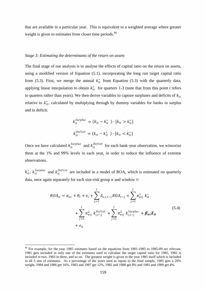
159
that are available in a particular year. This is equivalent to a weighted average where greater
weight is given to estimates from closer time periods.86
Stage 3: Estimating the determinants of the return on assets
The final stage of our analysis is to analyse the effects of capital ratio on the return on assets,
using a modified version of Equation (5.1), incorporating the long run target capital ratio
from (5.3). First, we merge the annual 𝑘𝑖𝑡∗ from Equation (5.3) with the quarterly data,
applying linear interpolation to obtain 𝑘𝑖𝑡∗ for quarters 1-3 (note that from this point t refers
to quarters rather than years). We then derive variables to capture surpluses and deficits of 𝑘𝑖𝑡
relative to 𝑘𝑖𝑡∗ , calculated by multiplying through by dummy variables for banks in surplus
and in deficit:
𝑘𝑖𝑡𝑆𝑢𝑟𝑝𝑙𝑢𝑠 = 𝑘𝑖𝑡 − 𝑘𝑖𝑡
∗ ∙ [𝑘𝑖𝑡 > 𝑘𝑖𝑡∗ ]
𝑘𝑖𝑡𝐷𝑒𝑓𝑖𝑐𝑖𝑡
= 𝑘𝑖𝑡 − 𝑘𝑖𝑡∗ ∙ [𝑘𝑖𝑡 < 𝑘𝑖𝑡
∗ ]
Once we have calculated 𝑘𝑖𝑡𝑆𝑢𝑟𝑝𝑙𝑢𝑠
and 𝑘𝑖𝑡𝐷𝑒𝑓𝑖𝑐𝑖𝑡
for each bank-year observation, we winsorize
them at the 1% and 99% levels in each year, in order to reduce the influence of extreme
observations.
𝑘𝑖𝑡∗ , 𝑘𝑖𝑡
𝑆𝑢𝑟𝑝𝑙𝑢𝑠 and 𝑘𝑖𝑡
𝐷𝑒𝑓𝑖𝑐𝑖𝑡 are included in a model of ROA, which is estimated on quarterly
data, once again separately for each size-risk group 𝜅 and window 𝜏:
𝑅𝑂𝐴𝑖𝑡 = 𝛼𝜅𝜏 + 𝜃𝑡 + 𝜐𝑖 + 𝛿𝜅 ,𝜏 ,𝑡−𝑗𝑅𝑂𝐴𝑡−𝑗
𝐽
𝑗=1
+ 𝜋𝜅𝜏𝑗1
𝐽
𝑗=1
𝑘𝑖𝑡∗
+ 𝜋𝜅𝜏𝑗2
𝐽
𝑗=1
𝑘𝑖 ,𝑡−𝑗𝐷𝑒𝑓𝑖𝑐𝑖𝑡
+ 𝜋𝜅𝜏𝑗3
𝐽
𝑗=1
𝑘𝑖 ,𝑡−𝑗𝑆𝑢𝑟𝑝𝑙𝑢𝑠 + 𝜷𝜿𝝉
′ 𝒁𝒊𝒕
+ 𝑒𝑖𝑡
(5.4)
86
For example, for the year 1985 estimates based on the equations from 1981-1985 to 1985-89 are relevant.
1981 gets included in only one of the estimates used to calculate the target capital ratio for 1985, 1982 is
included in two, 1983 in three, and so on. The greatest weight is given to the year 1985 itself which is included
in all 5 sets of estimates. As a percentage of the years used as inputs to the final sample, 1985 gets a 20%
weight, 1984 and 1986 get 16%, 1983 and 1987 get 12%, 1982 and 1988 get 8% and 1981 and 1989 get 4%.
160
In this equation 𝜋2 gives the long-run relationship, i.e. where 𝑘 = 𝑘∗, and 𝜋2 and 𝜋3 give the
short-run effects, where 𝑘∗ is fixed. If our hypothesis about the effect of capital on
profitability is correct, that banks tend to target their optimal capital ratios where profitability
is maximised, then 𝑘𝑖𝑡−1𝑆𝑢𝑟𝑝𝑙𝑢𝑠
should be negatively correlated with 𝑅𝑂𝐴𝑖𝑡 (𝜋3 < 0) and
𝑘𝑖𝑡−1𝐷𝑒𝑓𝑖𝑐𝑖𝑡
should be positively correlated with 𝑅𝑂𝐴𝑖𝑡 (𝜋2 > 0). We again estimate Equation
(5.5) using 5-year rolling windows. There are 20 time periods in each 5-year window, and 29
years in total (the first year, 1977, is lost due to the inclusion of (annual) lagged variables in
Equation (5.2). As before, equation (5.5) is estimated using two-step system GMM,
instrumenting lags of ROA. J is set to 4 to capture a full year of lags. As a robustness check,
in section 5.4.3 below we present results based on the fixed effects estimator.
5.4.2 Results
We show the detailed results from estimating our target capital ratio Equation (5.2) in Table
5.3, Table 5.4 and Table 5.5 for small banks, medium sized banks and big banks respectively,
each divided into three risk groups. Considering the large number of regression results, we
only show the long-run coefficients from Equation (5.3), and rather than showing results for
all 30 windows we only show those for selected windows spanning the whole range of our
sample period, 1977-1980, 1981-85, 1986-90, 1991-95, 1996-2000, 2001-05 and 2006-10.
Among those variables with most consistent explanatory value are ROA which is positively
correlated with k and SIZE which is negative, suggesting effects of size within the size
groups. BANKSHARE is positively correlated with k, suggesting that banks with a dominant
local market position tend to have higher capital ratios, but other market structure variables
have mixed sign and significance. Of the portfolio risk measures, CHARGE is positive and
significant for medium and high risk banks, whereas C&I, SDROE and RW are negative and
NPL is mixed in sign and significance. The latter finding may indicate that a riskier business
profile reduces the bank‘s charter value and therefore reduce incentives for holding higher
capital, or it could simply be that banks tend to target a given probability of default, so more
risk averse banks tend to have higher portfolio risk and higher capital (Jokipii and Milne
2009). Finally, AC has mixed sign and significance. The diagnostic tests produce rather
mixed results. The Arellano-Bond test for auto-correlation in differenced residuals indicate
that there is autocorrelation of order 1 but, for most samples not in order 2 which validates
161
the use of lagged levels of k and ROE as instruments. However, the Sargan and Hansen tests
generally reject the null hypothesis of exogeneity of the instrument set. This may be because
of the use of portfolio risk variables as explanatory variables, which are potentially
endogenous.
Having estimated the long-run determinants of the k, we proceed to calculate the long-run
target capital ratio using Equation (5.3).87
In Figure 5.5, we show the median k and target k
in each quarter (dashed and full lines respectively), separately for each group. Consistent
with the general rise in k shown in Figure 5.1 and Figure 5.2 above, the charts show that the k
rose substantially over our sample period across every level of portfolio risk and size. The k
and the target k are shown to move closely together over the sample period and both exhibit
the rise between the 1990s and the 2000s. We also show on the right axis the buffer used to
calculate 𝑘𝑖𝑡𝑆𝑢𝑟𝑝𝑙𝑢𝑠
and 𝑘𝑖𝑡𝐷𝑒𝑓𝑖𝑐𝑖𝑡
, in bands between the 10th
and 90th
percentiles (light gray) and
between the 25th
and 75th
percentiles (dark grey). For most groups and quarters, these lie
between +/- 2 percentage points, although they can be seen to rise and fall over time as banks
ks move around the target k over time. Most banks are below their target capital ratios in the
mid-1990s, consistent with the substantial rise in ks that was observed at that time. However,
k are not below target k in the mid- to late- 1980s, counter to the argument in Berger (1995)
that optimal ks were rising in this period; in fact for the high risk groups ks are generally
above their target levels in this period. This could reflect that the target ks are lagging
indicators of banks‘ optimal capital ratios and therefore may not capture the shift in
unobserved optimal capital ratios that took place.
87
The Im-Shin-Pesaran panel unit root test was used to test the null hypothesis that all of the panel units have
unit roots and this was rejected, consistent with the economic rationale that k should be stationary. However,
some of the regressions of equation (5.2) exhibit a high degree of autocorrelation of k, which may indicate that
the use of the partial adjustment model is invalid, since high values of aκτ2 produce implausibly large estimates
of the long-run coefficients (this can be seen, for example, in the estimates for group 1 in 1977-80 in Table 5.3
and group 7 in 1991-95 and 1996-2000 in Table 5.5). This suggests that a unit root may be relevant in some
subsamples, and I adopt the practical step of replacing the estimated target capital ratio with the 5-year moving
average of k for those windows with aκτ2 > 0.85 (approximately the value above which aκτ
2 is not significantly
different from one). This affects 19 out of 270 group-window pairs.
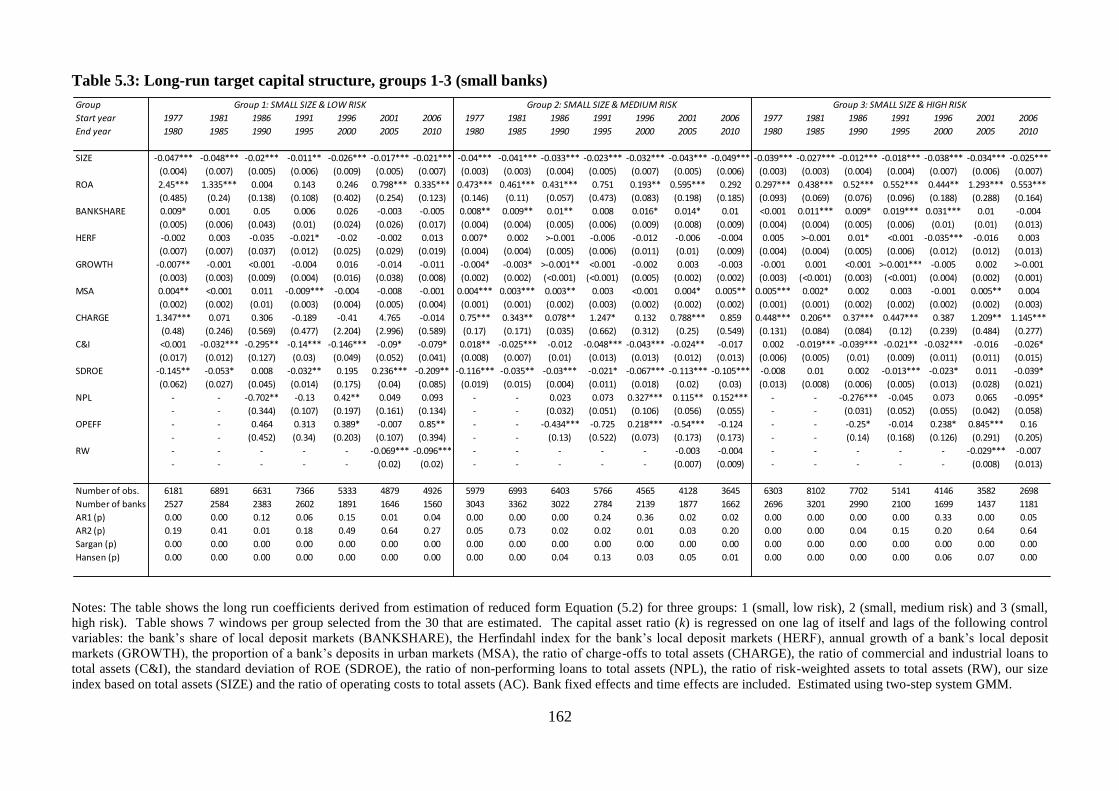
162
Table 5.3: Long-run target capital structure, groups 1-3 (small banks)
Notes: The table shows the long run coefficients derived from estimation of reduced form Equation (5.2) for three groups: 1 (small, low risk), 2 (small, medium risk) and 3 (small,
high risk). Table shows 7 windows per group selected from the 30 that are estimated. The capital asset ratio (k) is regressed on one lag of itself and lags of the following control
variables: the bank‘s share of local deposit markets (BANKSHARE), the Herfindahl index for the bank‘s local deposit markets (HERF), annual growth of a bank‘s local deposit
markets (GROWTH), the proportion of a bank‘s deposits in urban markets (MSA), the ratio of charge-offs to total assets (CHARGE), the ratio of commercial and industrial loans to
total assets (C&I), the standard deviation of ROE (SDROE), the ratio of non-performing loans to total assets (NPL), the ratio of risk-weighted assets to total assets (RW), our size
index based on total assets (SIZE) and the ratio of operating costs to total assets (AC). Bank fixed effects and time effects are included. Estimated using two-step system GMM.
Group
Start year 1977 1981 1986 1991 1996 2001 2006 1977 1981 1986 1991 1996 2001 2006 1977 1981 1986 1991 1996 2001 2006
End year 1980 1985 1990 1995 2000 2005 2010 1980 1985 1990 1995 2000 2005 2010 1980 1985 1990 1995 2000 2005 2010
SIZE -0.047*** -0.048*** -0.02*** -0.011** -0.026*** -0.017*** -0.021*** -0.04*** -0.041*** -0.033*** -0.023*** -0.032*** -0.043*** -0.049*** -0.039*** -0.027*** -0.012*** -0.018*** -0.038*** -0.034*** -0.025***
(0.004) (0.007) (0.005) (0.006) (0.009) (0.005) (0.007) (0.003) (0.003) (0.004) (0.005) (0.007) (0.005) (0.006) (0.003) (0.003) (0.004) (0.004) (0.007) (0.006) (0.007)
ROA 2.45*** 1.335*** 0.004 0.143 0.246 0.798*** 0.335*** 0.473*** 0.461*** 0.431*** 0.751 0.193** 0.595*** 0.292 0.297*** 0.438*** 0.52*** 0.552*** 0.444** 1.293*** 0.553***
(0.485) (0.24) (0.138) (0.108) (0.402) (0.254) (0.123) (0.146) (0.11) (0.057) (0.473) (0.083) (0.198) (0.185) (0.093) (0.069) (0.076) (0.096) (0.188) (0.288) (0.164)
BANKSHARE 0.009* 0.001 0.05 0.006 0.026 -0.003 -0.005 0.008** 0.009** 0.01** 0.008 0.016* 0.014* 0.01 <0.001 0.011*** 0.009* 0.019*** 0.031*** 0.01 -0.004
(0.005) (0.006) (0.043) (0.01) (0.024) (0.026) (0.017) (0.004) (0.004) (0.005) (0.006) (0.009) (0.008) (0.009) (0.004) (0.004) (0.005) (0.006) (0.01) (0.01) (0.013)
HERF -0.002 0.003 -0.035 -0.021* -0.02 -0.002 0.013 0.007* 0.002 >-0.001 -0.006 -0.012 -0.006 -0.004 0.005 >-0.001 0.01* <0.001 -0.035*** -0.016 0.003
(0.007) (0.007) (0.037) (0.012) (0.025) (0.029) (0.019) (0.004) (0.004) (0.005) (0.006) (0.011) (0.01) (0.009) (0.004) (0.004) (0.005) (0.006) (0.012) (0.012) (0.013)
GROWTH -0.007** -0.001 <0.001 -0.004 0.016 -0.014 -0.011 -0.004* -0.003* >-0.001** <0.001 -0.002 0.003 -0.003 -0.001 0.001 <0.001 >-0.001*** -0.005 0.002 >-0.001
(0.003) (0.003) (0.009) (0.004) (0.016) (0.038) (0.008) (0.002) (0.002) (<0.001) (<0.001) (0.005) (0.002) (0.002) (0.003) (<0.001) (0.003) (<0.001) (0.004) (0.002) (0.001)
MSA 0.004** <0.001 0.011 -0.009*** -0.004 -0.008 -0.001 0.004*** 0.003*** 0.003** 0.003 <0.001 0.004* 0.005** 0.005*** 0.002* 0.002 0.003 -0.001 0.005** 0.004
(0.002) (0.002) (0.01) (0.003) (0.004) (0.005) (0.004) (0.001) (0.001) (0.002) (0.003) (0.002) (0.002) (0.002) (0.001) (0.001) (0.002) (0.002) (0.002) (0.002) (0.003)
CHARGE 1.347*** 0.071 0.306 -0.189 -0.41 4.765 -0.014 0.75*** 0.343** 0.078** 1.247* 0.132 0.788*** 0.859 0.448*** 0.206** 0.37*** 0.447*** 0.387 1.209** 1.145***
(0.48) (0.246) (0.569) (0.477) (2.204) (2.996) (0.589) (0.17) (0.171) (0.035) (0.662) (0.312) (0.25) (0.549) (0.131) (0.084) (0.084) (0.12) (0.239) (0.484) (0.277)
C&I <0.001 -0.032*** -0.295** -0.14*** -0.146*** -0.09* -0.079* 0.018** -0.025*** -0.012 -0.048*** -0.043*** -0.024** -0.017 0.002 -0.019*** -0.039*** -0.021** -0.032*** -0.016 -0.026*
(0.017) (0.012) (0.127) (0.03) (0.049) (0.052) (0.041) (0.008) (0.007) (0.01) (0.013) (0.013) (0.012) (0.013) (0.006) (0.005) (0.01) (0.009) (0.011) (0.011) (0.015)
SDROE -0.145** -0.053* 0.008 -0.032** 0.195 0.236*** -0.209** -0.116*** -0.035** -0.03*** -0.021* -0.067*** -0.113*** -0.105*** -0.008 0.01 0.002 -0.013*** -0.023* 0.011 -0.039*
(0.062) (0.027) (0.045) (0.014) (0.175) (0.04) (0.085) (0.019) (0.015) (0.004) (0.011) (0.018) (0.02) (0.03) (0.013) (0.008) (0.006) (0.005) (0.013) (0.028) (0.021)
NPL - - -0.702** -0.13 0.42** 0.049 0.093 - - 0.023 0.073 0.327*** 0.115** 0.152*** - - -0.276*** -0.045 0.073 0.065 -0.095*
- - (0.344) (0.107) (0.197) (0.161) (0.134) - - (0.032) (0.051) (0.106) (0.056) (0.055) - - (0.031) (0.052) (0.055) (0.042) (0.058)
OPEFF - - 0.464 0.313 0.389* -0.007 0.85** - - -0.434*** -0.725 0.218*** -0.54*** -0.124 - - -0.25* -0.014 0.238* 0.845*** 0.16
- - (0.452) (0.34) (0.203) (0.107) (0.394) - - (0.13) (0.522) (0.073) (0.173) (0.173) - - (0.14) (0.168) (0.126) (0.291) (0.205)
RW - - - - - -0.069*** -0.096*** - - - - - -0.003 -0.004 - - - - - -0.029*** -0.007
- - - - - (0.02) (0.02) - - - - - (0.007) (0.009) - - - - - (0.008) (0.013)
Number of obs. 6181 6891 6631 7366 5333 4879 4926 5979 6993 6403 5766 4565 4128 3645 6303 8102 7702 5141 4146 3582 2698
Number of banks 2527 2584 2383 2602 1891 1646 1560 3043 3362 3022 2784 2139 1877 1662 2696 3201 2990 2100 1699 1437 1181
AR1 (p) 0.00 0.00 0.12 0.06 0.15 0.01 0.04 0.00 0.00 0.00 0.24 0.36 0.02 0.02 0.00 0.00 0.00 0.00 0.33 0.00 0.05
AR2 (p) 0.19 0.41 0.01 0.18 0.49 0.64 0.27 0.05 0.73 0.02 0.02 0.01 0.03 0.20 0.00 0.00 0.04 0.15 0.20 0.64 0.64
Sargan (p) 0.00 0.00 0.00 0.00 0.00 0.00 0.00 0.00 0.00 0.00 0.00 0.00 0.00 0.00 0.00 0.00 0.00 0.00 0.00 0.00 0.00
Hansen (p) 0.00 0.00 0.00 0.00 0.00 0.00 0.00 0.00 0.00 0.04 0.13 0.03 0.05 0.01 0.00 0.00 0.00 0.00 0.06 0.07 0.00
Group 1: SMALL SIZE & LOW RISK Group 2: SMALL SIZE & MEDIUM RISK Group 3: SMALL SIZE & HIGH RISK
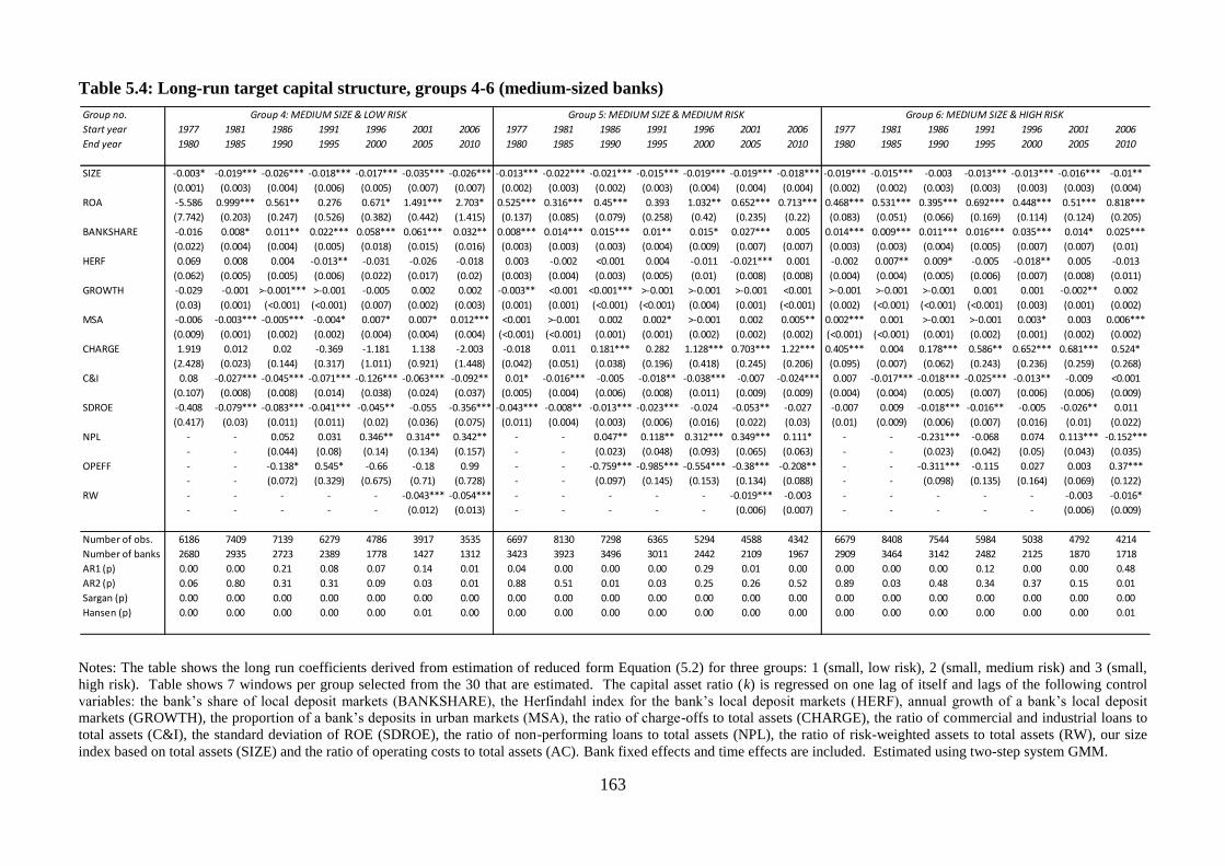
163
Table 5.4: Long-run target capital structure, groups 4-6 (medium-sized banks)
Notes: The table shows the long run coefficients derived from estimation of reduced form Equation (5.2) for three groups: 1 (small, low risk), 2 (small, medium risk) and 3 (small,
high risk). Table shows 7 windows per group selected from the 30 that are estimated. The capital asset ratio (k) is regressed on one lag of itself and lags of the following control
variables: the bank‘s share of local deposit markets (BANKSHARE), the Herfindahl index for the bank‘s local deposit markets (HERF), annual growth of a bank‘s local deposit
markets (GROWTH), the proportion of a bank‘s deposits in urban markets (MSA), the ratio of charge-offs to total assets (CHARGE), the ratio of commercial and industrial loans to
total assets (C&I), the standard deviation of ROE (SDROE), the ratio of non-performing loans to total assets (NPL), the ratio of risk-weighted assets to total assets (RW), our size
index based on total assets (SIZE) and the ratio of operating costs to total assets (AC). Bank fixed effects and time effects are included. Estimated using two-step system GMM.
Group no.
Start year 1977 1981 1986 1991 1996 2001 2006 1977 1981 1986 1991 1996 2001 2006 1977 1981 1986 1991 1996 2001 2006
End year 1980 1985 1990 1995 2000 2005 2010 1980 1985 1990 1995 2000 2005 2010 1980 1985 1990 1995 2000 2005 2010
SIZE -0.003* -0.019*** -0.026*** -0.018*** -0.017*** -0.035*** -0.026*** -0.013*** -0.022*** -0.021*** -0.015*** -0.019*** -0.019*** -0.018*** -0.019*** -0.015*** -0.003 -0.013*** -0.013*** -0.016*** -0.01**
(0.001) (0.003) (0.004) (0.006) (0.005) (0.007) (0.007) (0.002) (0.003) (0.002) (0.003) (0.004) (0.004) (0.004) (0.002) (0.002) (0.003) (0.003) (0.003) (0.003) (0.004)
ROA -5.586 0.999*** 0.561** 0.276 0.671* 1.491*** 2.703* 0.525*** 0.316*** 0.45*** 0.393 1.032** 0.652*** 0.713*** 0.468*** 0.531*** 0.395*** 0.692*** 0.448*** 0.51*** 0.818***
(7.742) (0.203) (0.247) (0.526) (0.382) (0.442) (1.415) (0.137) (0.085) (0.079) (0.258) (0.42) (0.235) (0.22) (0.083) (0.051) (0.066) (0.169) (0.114) (0.124) (0.205)
BANKSHARE -0.016 0.008* 0.011** 0.022*** 0.058*** 0.061*** 0.032** 0.008*** 0.014*** 0.015*** 0.01** 0.015* 0.027*** 0.005 0.014*** 0.009*** 0.011*** 0.016*** 0.035*** 0.014* 0.025***
(0.022) (0.004) (0.004) (0.005) (0.018) (0.015) (0.016) (0.003) (0.003) (0.003) (0.004) (0.009) (0.007) (0.007) (0.003) (0.003) (0.004) (0.005) (0.007) (0.007) (0.01)
HERF 0.069 0.008 0.004 -0.013** -0.031 -0.026 -0.018 0.003 -0.002 <0.001 0.004 -0.011 -0.021*** 0.001 -0.002 0.007** 0.009* -0.005 -0.018** 0.005 -0.013
(0.062) (0.005) (0.005) (0.006) (0.022) (0.017) (0.02) (0.003) (0.004) (0.003) (0.005) (0.01) (0.008) (0.008) (0.004) (0.004) (0.005) (0.006) (0.007) (0.008) (0.011)
GROWTH -0.029 -0.001 >-0.001*** >-0.001 -0.005 0.002 0.002 -0.003** <0.001 <0.001*** >-0.001 >-0.001 >-0.001 <0.001 >-0.001 >-0.001 >-0.001 0.001 0.001 -0.002** 0.002
(0.03) (0.001) (<0.001) (<0.001) (0.007) (0.002) (0.003) (0.001) (0.001) (<0.001) (<0.001) (0.004) (0.001) (<0.001) (0.002) (<0.001) (<0.001) (<0.001) (0.003) (0.001) (0.002)
MSA -0.006 -0.003*** -0.005*** -0.004* 0.007* 0.007* 0.012*** <0.001 >-0.001 0.002 0.002* >-0.001 0.002 0.005** 0.002*** 0.001 >-0.001 >-0.001 0.003* 0.003 0.006***
(0.009) (0.001) (0.002) (0.002) (0.004) (0.004) (0.004) (<0.001) (<0.001) (0.001) (0.001) (0.002) (0.002) (0.002) (<0.001) (<0.001) (0.001) (0.002) (0.001) (0.002) (0.002)
CHARGE 1.919 0.012 0.02 -0.369 -1.181 1.138 -2.003 -0.018 0.011 0.181*** 0.282 1.128*** 0.703*** 1.22*** 0.405*** 0.004 0.178*** 0.586** 0.652*** 0.681*** 0.524*
(2.428) (0.023) (0.144) (0.317) (1.011) (0.921) (1.448) (0.042) (0.051) (0.038) (0.196) (0.418) (0.245) (0.206) (0.095) (0.007) (0.062) (0.243) (0.236) (0.259) (0.268)
C&I 0.08 -0.027*** -0.045*** -0.071*** -0.126*** -0.063*** -0.092** 0.01* -0.016*** -0.005 -0.018** -0.038*** -0.007 -0.024*** 0.007 -0.017*** -0.018*** -0.025*** -0.013** -0.009 <0.001
(0.107) (0.008) (0.008) (0.014) (0.038) (0.024) (0.037) (0.005) (0.004) (0.006) (0.008) (0.011) (0.009) (0.009) (0.004) (0.004) (0.005) (0.007) (0.006) (0.006) (0.009)
SDROE -0.408 -0.079*** -0.083*** -0.041*** -0.045** -0.055 -0.356*** -0.043*** -0.008** -0.013*** -0.023*** -0.024 -0.053** -0.027 -0.007 0.009 -0.018*** -0.016** -0.005 -0.026** 0.011
(0.417) (0.03) (0.011) (0.011) (0.02) (0.036) (0.075) (0.011) (0.004) (0.003) (0.006) (0.016) (0.022) (0.03) (0.01) (0.009) (0.006) (0.007) (0.016) (0.01) (0.022)
NPL - - 0.052 0.031 0.346** 0.314** 0.342** - - 0.047** 0.118** 0.312*** 0.349*** 0.111* - - -0.231*** -0.068 0.074 0.113*** -0.152***
- - (0.044) (0.08) (0.14) (0.134) (0.157) - - (0.023) (0.048) (0.093) (0.065) (0.063) - - (0.023) (0.042) (0.05) (0.043) (0.035)
OPEFF - - -0.138* 0.545* -0.66 -0.18 0.99 - - -0.759*** -0.985*** -0.554*** -0.38*** -0.208** - - -0.311*** -0.115 0.027 0.003 0.37***
- - (0.072) (0.329) (0.675) (0.71) (0.728) - - (0.097) (0.145) (0.153) (0.134) (0.088) - - (0.098) (0.135) (0.164) (0.069) (0.122)
RW - - - - - -0.043*** -0.054*** - - - - - -0.019*** -0.003 - - - - - -0.003 -0.016*
- - - - - (0.012) (0.013) - - - - - (0.006) (0.007) - - - - - (0.006) (0.009)
Number of obs. 6186 7409 7139 6279 4786 3917 3535 6697 8130 7298 6365 5294 4588 4342 6679 8408 7544 5984 5038 4792 4214
Number of banks 2680 2935 2723 2389 1778 1427 1312 3423 3923 3496 3011 2442 2109 1967 2909 3464 3142 2482 2125 1870 1718
AR1 (p) 0.00 0.00 0.21 0.08 0.07 0.14 0.01 0.04 0.00 0.00 0.00 0.29 0.01 0.00 0.00 0.00 0.00 0.12 0.00 0.00 0.48
AR2 (p) 0.06 0.80 0.31 0.31 0.09 0.03 0.01 0.88 0.51 0.01 0.03 0.25 0.26 0.52 0.89 0.03 0.48 0.34 0.37 0.15 0.01
Sargan (p) 0.00 0.00 0.00 0.00 0.00 0.00 0.00 0.00 0.00 0.00 0.00 0.00 0.00 0.00 0.00 0.00 0.00 0.00 0.00 0.00 0.00
Hansen (p) 0.00 0.00 0.00 0.00 0.00 0.01 0.00 0.00 0.00 0.00 0.00 0.00 0.00 0.00 0.00 0.00 0.00 0.00 0.00 0.00 0.01
Group 4: MEDIUM SIZE & LOW RISK Group 5: MEDIUM SIZE & MEDIUM RISK Group 6: MEDIUM SIZE & HIGH RISK

164
Table 5.5: Long-run target capital structure, groups 7-9 (big banks)
Notes: The table shows the long run coefficients derived from estimation of reduced form Equation (5.2) for three groups: 1 (small, low risk), 2 (small, medium risk) and 3 (small,
high risk). Table shows 7 windows per group selected from the 30 that are estimated. The capital asset ratio (k) is regressed on one lag of itself and lags of the following control
variables: the bank‘s share of local deposit markets (BANKSHARE), the Herfindahl index for the bank‘s local deposit markets (HERF), annual growth of a bank‘s local deposit
markets (GROWTH), the proportion of a bank‘s deposits in urban markets (MSA), the ratio of charge-offs to total assets (CHARGE), the ratio of commercial and industrial loans to
total assets (C&I), the standard deviation of ROE (SDROE), the ratio of non-performing loans to total assets (NPL), the ratio of risk-weighted assets to total assets (RW), our size
index based on total assets (SIZE) and the ratio of operating costs to total assets (AC). Bank fixed effects and time effects are included. Estimated using two-step system GMM.
Group no.
Start year 1977 1981 1986 1991 1996 2001 2006 1977 1981 1986 1991 1996 2001 2006 1977 1981 1986 1991 1996 2001 2006
End year 1980 1985 1990 1995 2000 2005 2010 1980 1985 1990 1995 2000 2005 2010 1980 1985 1990 1995 2000 2005 2010
SIZE -0.006 -0.011** -0.02*** -0.016*** -0.008 -0.01** -0.016 -0.03*** -0.034*** -0.027*** -0.018*** -0.013* -0.01** -0.006 -0.038*** -0.028*** -0.018** -0.02*** -0.002 0.001 0.015***
(0.006) (0.004) (0.007) (0.006) (0.008) (0.004) (0.011) (0.007) (0.002) (0.006) (0.004) (0.007) (0.004) (0.004) (0.009) (0.005) (0.009) (0.006) (0.003) (0.003) (0.004)
ROA 35.868 4.34 2.112*** -15.422 55.798 -1.816*** 0.524 0.532* 0.714*** 0.561** 2.845* 0.938 0.21 1.749** 0.47*** 0.724*** 1.199** 0.598*** 0.23 1.131*** 0.646***
(366.913) (3.024) (0.775) (23.756) (443.565) (0.669) (0.829) (0.314) (0.123) (0.236) (1.536) (0.785) (0.298) (0.749) (0.164) (0.104) (0.592) (0.124) (0.212) (0.318) (0.202)
BANKSHARE 0.145 0.042 0.007 0.159 -0.014 0.067** 0.018 0.008* 0.011*** 0.011*** 0.025* 0.007 0.01 -0.016 0.01*** 0.005 0.004 -0.002 0.002 -0.013 -0.015
(1.488) (0.029) (0.006) (0.27) (0.36) (0.03) (0.016) (0.004) (0.003) (0.004) (0.013) (0.01) (0.011) (0.012) (0.004) (0.003) (0.006) (0.004) (0.008) (0.013) (0.009)
HERF -0.334 -0.033 0.004 -0.085 -0.249 -0.057 -0.034* <0.001 -0.004 -0.005 -0.021 <0.001 -0.002 0.008 -0.005 0.002 0.014* -0.001 0.006 0.002 0.007
(3.508) (0.032) (0.008) (0.174) (1.99) (0.041) (0.019) (0.005) (0.004) (0.005) (0.013) (0.014) (0.012) (0.01) (0.005) (0.004) (0.009) (0.005) (0.009) (0.019) (0.01)
GROWTH 0.049 0.002 <0.001 0.002 0.084 0.002 0.004 -0.002 <0.001 >-0.001 <0.001 0.009 0.003 0.005 -0.003* <0.001 -0.001* <0.001 0.001 -0.009 <0.001
(0.554) (0.003) (<0.001) (0.007) (0.719) (0.008) (0.005) (0.001) (<0.001) (<0.001) (<0.001) (0.008) (0.007) (0.014) (0.002) (0.001) (<0.001) (<0.001) (0.003) (0.017) (0.003)
MSA 0.045 0.004 >-0.001 0.027 0.11 0.003 <0.001 <0.001 -0.001 >-0.001 0.009 >-0.001 -0.001 0.002 <0.001 >-0.001 -0.002 -0.003** -0.004** -0.001 -0.002
(0.453) (0.004) (0.002) (0.055) (0.879) (0.006) (0.005) (0.001) (<0.001) (0.001) (0.005) (0.003) (0.003) (0.003) (0.001) (<0.001) (0.002) (0.001) (0.002) (0.003) (0.003)
CHARGE 6.13 0.118 0.342 -4.19 26.433 1.602 -0.804 0.569** 0.326*** 0.317** 1.76* 1.323** 0.246 2.02*** 0.022 0.022 0.461 0.364** 0.53*** 0.879*** 0.391**
(65.195) (0.54) (0.503) (6.645) (217.958) (1.612) (1.169) (0.247) (0.111) (0.145) (0.935) (0.626) (0.305) (0.478) (0.016) (0.026) (0.364) (0.143) (0.17) (0.281) (0.19)
C&I -0.408 -0.071 -0.037** -0.241 -1.247 -0.082** -0.041 -0.003 -0.006* -0.019*** -0.037** -0.026* -0.014 0.017 0.013*** -0.01** -0.009 -0.003 0.005 -0.003 0.01
(4.36) (0.049) (0.015) (0.388) (9.547) (0.038) (0.035) (0.006) (0.004) (0.005) (0.016) (0.013) (0.008) (0.012) (0.005) (0.004) (0.009) (0.006) (0.009) (0.012) (0.01)
SDROE -0.563 0.113 -0.052 -0.199 -0.144 -0.121 0.24 -0.075*** -0.069*** -0.018 -0.036** 0.023 -0.048 0.054 -0.032** 0.011 0.011 -0.015 -0.009 0.008 -0.021
(3.993) (0.21) (0.04) (0.224) (0.852) (0.241) (0.199) (0.014) (0.012) (0.011) (0.014) (0.029) (0.036) (0.082) (0.014) (0.01) (0.027) (0.009) (0.012) (0.031) (0.029)
NPL - - 0.179 -1.916 5.328 0.439 0.426* - - 0.155*** 0.31*** 0.501*** 0.192*** 0.163* - - -0.227** 0.002 0.141** 0.228*** -0.222***
- - (0.175) (3.666) (39.544) (0.374) (0.25) - - (0.037) (0.107) (0.141) (0.072) (0.088) - - (0.09) (0.035) (0.057) (0.072) (0.038)
OPEFF - - -0.477* -0.214 -14.237 2.082* 0.56 - - -0.467*** -0.565*** -0.53** -0.204 -0.225* - - -0.215** -0.152** 0.133 0.144 0.262***
- - (0.261) (1.826) (116.818) (1.168) (0.699) - - (0.098) (0.207) (0.207) (0.166) (0.135) - - (0.091) (0.077) (0.081) (0.133) (0.09)
RW - - - - - -0.077*** -0.04 - - - - - -0.005 -0.009 - - - - - 0.002 <0.001
- - - - - (0.026) (0.025) - - - - - (0.006) (0.012) - - - - - (0.01) (0.01)
Number of obs. 5041 6695 6279 4103 3980 3864 2774 6913 8986 8373 6647 5195 4528 4113 6585 7879 7219 7778 6082 5066 5385
Number of banks 2248 2641 2383 1643 1426 1295 1016 3252 3828 3576 2832 2241 1897 1823 2648 2935 2912 2744 2280 1743 1844
AR1 (p) 0.00 0.00 0.91 0.06 0.03 0.00 0.32 0.16 0.00 0.10 0.00 0.01 0.06 0.43 0.32 0.13 0.09 0.08 0.00 0.00 0.01
AR2 (p) 0.05 0.69 0.77 0.03 0.33 0.07 0.31 0.46 0.26 0.05 0.00 0.25 0.09 0.25 0.21 0.31 0.58 0.02 0.12 0.02 0.04
Sargan (p) 0.00 0.00 0.00 0.00 0.00 0.00 0.00 0.00 0.00 0.00 0.00 0.00 0.00 0.00 0.00 0.00 0.00 0.00 0.00 0.00 0.00
Hansen (p) 0.00 0.00 0.00 0.00 0.00 0.00 0.00 0.00 0.00 0.00 0.00 0.00 0.00 0.05 0.00 0.00 0.00 0.00 0.00 0.00 0.00
Group 7: BIG SIZE & LOW RISK Group 8: BIG SIZE & MEDIUM RISK Group 9: BIG SIZE & HIGH RISK

165
Figure 5.5: Charts of median k and median k* , and buffer at the 10th, 25th, 75th and 90th percentiles
Notes: Charts show the medians of the actual k and kit∗ (left axis), estimated using equations (5.2) and (5.3), full details of which are given in the notes to Table 5.3, Table 5.4 and
Table 5.5. We also show the buffer of k relative to kit∗ at the 10
th, 25
th, 75
th and 90
th percentiles (right axis).
-5%
-4%
-3%
-2%
-1%
0%
1%
2%
3%
4%
5%
4%
6%
8%
10%
12%
14%
16%
Group 1: small size, low risk
Buffer, quantiles 25-75 (left axis) Buffer, quantiles 10-90 (left axis)
k k*
-5%
-4%
-3%
-2%
-1%
0%
1%
2%
3%
4%
5%
4%
5%
6%
7%
8%
9%
10%
11%
12%
Group 2: small size, medium risk
Buffer, quantiles 25-75 (left axis) Buffer, quantiles 10-90 (left axis)
k k*
-5%
-4%
-3%
-2%
-1%
0%
1%
2%
3%
4%
5%
4%
5%
6%
7%
8%
9%
10%
11%
Group 3: small size, high risk
Buffer, quantiles 25-75 (left axis) Buffer, quantiles 10-90 (left axis)
k k*
-5%
-4%
-3%
-2%
-1%
0%
1%
2%
3%
4%
5%
4%
5%
6%
7%
8%
9%
10%
11%
12%
Group 4: medium size, low risk
Buffer, quantiles 25-75 (left axis) Buffer, quantiles 10-90 (left axis)
k k*
-5%
-4%
-3%
-2%
-1%
0%
1%
2%
3%
4%
5%
4%
5%
6%
7%
8%
9%
10%
11%
Group 4: medium size, medium risk
Buffer, quantiles 25-75 (left axis) Buffer, quantiles 10-90 (left axis)
k k*
-5%
-4%
-3%
-2%
-1%
0%
1%
2%
3%
4%
5%
4%
5%
6%
7%
8%
9%
10%
Group 6: medium size, high risk
Buffer, quantiles 25-75 (left axis) Buffer, quantiles 10-90 (left axis)
k k*
-5%
-4%
-3%
-2%
-1%
0%
1%
2%
3%
4%
5%
4%
5%
6%
7%
8%
9%
10%
11%
Group 7: big size, low risk
Buffer, quantiles 25-75 (left axis) Buffer, quantiles 10-90 (left axis)
k k*
-5%
-4%
-3%
-2%
-1%
0%
1%
2%
3%
4%
5%
4%
5%
6%
7%
8%
9%
10%
11%
Group 8: big size, medium risk
Buffer, quantiles 25-75 (left axis) Buffer, quantiles 10-90 (left axis)
k k*
-5%
-4%
-3%
-2%
-1%
0%
1%
2%
3%
4%
5%
4%
5%
6%
7%
8%
9%
10%
11%
Group 9: big size, high risk
Buffer, quantiles 25-75 (left axis) Buffer, quantiles 10-90 (left axis)
k k*

166
Next we proceed to our estimation of equation (5.5) which shows the relationship between
ROA and the three capital variables 𝒌𝒊𝒕∗ , 𝒌𝒊𝒕
𝑺𝒖𝒓𝒑𝒍𝒖𝒔 and 𝒌𝒊𝒕
𝑫𝒆𝒇𝒊𝒄𝒊𝒕, as well as the control variables
for portfolio risk and market structure. As a reminder, the target capital ratio was estimated
using equation (5.2) and has been interpolated from annual data to quarterly data in order to
estimate the ROA regression (5.5). We show the full results of estimating equation (5.5) in
Table 5.6, Table 5.7 and Table 5.8 for small, medium and large banks respectively, for
selected time windows as above. We then chart the total coefficients on the capital variables
in (5.5) in Figure 5.6. Overall, the long-run target capital ratio is positively correlated with
lagged ROA; this is not surprising since in the majority of the target capital regression the
long-run coefficient was also positive. 𝒌𝒊𝒕𝑫𝒆𝒇𝒊𝒄𝒊𝒕
is mostly positive as expected, but is also
negative for a large number of banks, whereas 𝒌𝒊𝒕𝑺𝒖𝒓𝒑𝒍𝒖𝒔
is consistently negative and strongly
significant.
We first examine the sample period 1983-89 used by Berger (1995). If the ―expected
bankruptcy costs‖ hypothesis in that paper is correct, then we would expect banks with a
deficit of capital relative to target to exhibit 𝝅𝟐 < 0. Inspection of Figure 5.6 shows that this
is observed, but only for the highest risk groups (3, 6, 9), which is consistent with the idea
that the riskiest banks would be under pressure from the market to increase their capital ratios
under stressed market conditions. For the other groups of banks, there is no evidence that
banks with low capital relative to their long-run targets are able to increase ROA by raising k
any more than other banks, which calls into question whether the ―expected bankruptcy
costs‖ hypothesis is relevant for these banks. We also find that during this period, banks with
a capital surplus relative to the long-run target are able to increase profitability by reducing
capital ratios (𝝅𝟑 < 0). This indicates that banks with relatively high capital ratios were able
to increase ROA by reducing k, at least in the short run. This validates our more
heterogeneous specification, since controlling only for k would not reveal this interesting
finding.
The next period of our analysis is the 1990s and early 2000s. As a reminder, our analysis
above showed that this is a period of rapidly rising capital ratios and strong profitability. For
small banks, a deficit of capital is generally associated with a positive k-ROA relationship
though the results are fairly weak and only observed for the low and medium risk groups. A
surplus of capital has a coefficient that is strong and consistently negative for all three groups
of small banks, suggesting that banks with high capital ratios were able to raise ROA by
167
reducing k. For both big and medium sized banks during this period there is a positive
though weak relationship (generally not significantly different from zero) for medium and
high risk banks with a capital deficit, and again a capital surplus is linked to a strongly
negative and statistically significant relationship. For all nine groups, the coefficient on the
long-run target k, 𝝅𝟏, is positive and significant. These results offer some insight into the
reasons for the increase in capital ratios during this period. While capital ratios are rising
strongly across the sample period, low capital banks do not improve their profitability by
increasing their capital ratios, at least in the short run, and this is true for low and high risk
banks. Thus the results do not support the contention of Flannery and Rangan (2008) that
weakening of implicit government guarantees increased the capital demanded by investors in
this period. The long-run co-movement of k and ROA is strongly positive, supporting the idea
that high profitability was driving higher capital ratios during this period, rather than the
other way around.
Finally, we examine the results for the recent crisis period, 2007-2010. As noted above, in
this period banks suffered substantial losses and have received unprecedented levels of
official support. Capital ratios have also come under pressure as banks seek to show their
balance sheets are solvent. However, our findings do not support the idea that banks with
low capital relative to long-run target levels were able to increase their ROA, and this was
true as much for high risk as for low risk banks (with the exception of small high risk banks
for whom the coefficient 𝝅𝟐 is significantly positive). The long-run target capital was
positively linked to capital but to nothing like the same extent that was observed in the 1980s
crisis. For most groups, it remains true in this period that banks with high capital ratios can
improve profitability by reducing their capital ratios. These results are slightly surprising
coming from a period of huge turmoil in the financial sector. One possible explanation of
these results is that official support and, indeed, injections of capital by the government
directly into troubled banks, have softened the effects of market discipline in this period.
One possible interpretation of the weak results for capital deficits, relative to capital
surpluses, is the role of regulatory capital requirements. If banks set their long-run target
capital ratio as a buffer over the capital requirements, then this implies that falling below the
target would be costly for the bank due to the risk of supervisory intervention (see Milne and
Whalley 2002 and other references cited in 5.2.1 above). If investors know and care about
these supervisory costs, then they would punish banks that have capital deficits, suggesting
lower profitability. Hence, the result is a modified version of the trade off theory where
168
regulation causes value to be upwards sloping in capital below the optimal capital ratio.
However, if investors do not price in the costs of supervisory intervention, for example
because they are unaware of supervisory activities (Berger et al 2000) or because they believe
they will be shielded from losses by government assistance, then the result (assuming capital
requirements are high enough to be binding on the bank) is that even below the long-run
target capital ratio profitability may be negatively correlated with capital, since investors see
the capital requirements as value-destroying. This may suggest why deficits of capital are
often negatively or non-correlated with capital ratios.
Finally, we summarise briefly the other control variables, shown in Table 5.6, Table 5.7 and
Table 5.8. Lagged ROA is consistently positive and highly significant, verifying the use of
the dynamic specification. Size and the measures of market power are mostly positive
although of mixed significance, suggesting that large banks with more local market power are
more profitable. As expected, the ex ante measures of risk (SDROE, C&I and RW) are
positively related to ROA, suggesting that more risky portfolios are associated with higher
profitability, whereas ex post measures of risk (NPL, CHARGE) are negatively related to
profitability, although in general the risk measures have mixed statistical significance.
Operating efficiency (AC) is of mixed sign and significance. Turning to the diagnostic tests,
although the tests for auto correlation (AR1 and AR2) show the desired results, the Sargan
and Hansen tests of over-identifying restrictions reject the null hypothesis of exogeneity of
the instruments. This suggests that the GMM method may not be an effective solution to the
lagged dependent variable bias, and in the robustness tests section below, we show results
based on the fixed effects estimator.
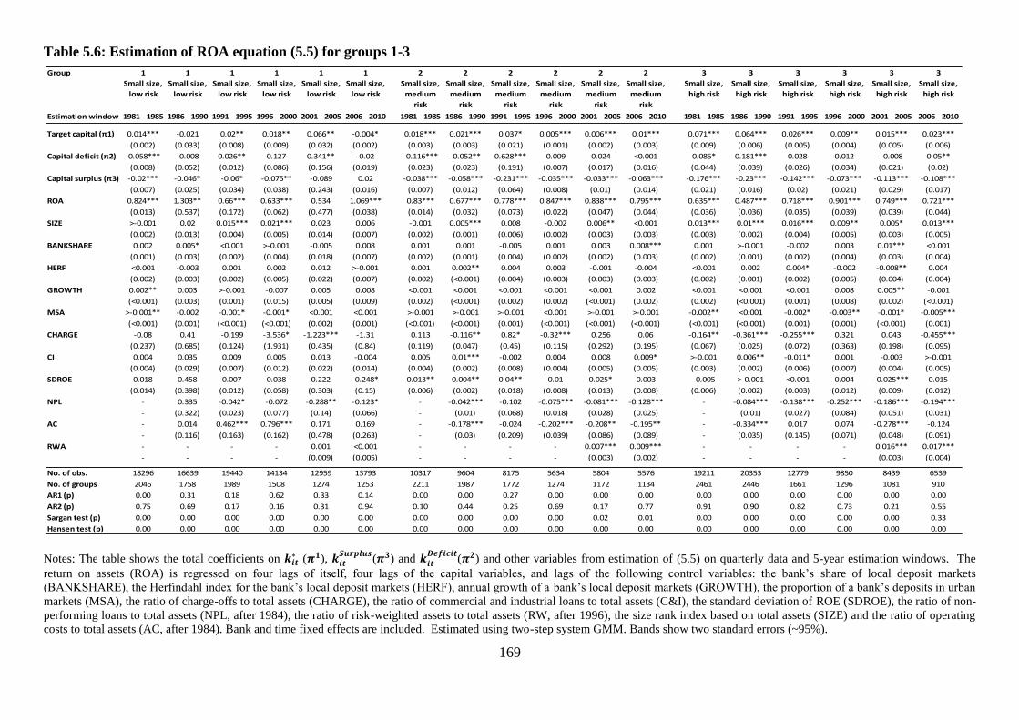
169
Table 5.6: Estimation of ROA equation (5.5) for groups 1-3
Notes: The table shows the total coefficients on 𝒌𝒊𝒕∗ (𝝅𝟏), 𝒌𝒊𝒕
𝑺𝒖𝒓𝒑𝒍𝒖𝒔(𝝅𝟑) and 𝒌𝒊𝒕
𝑫𝒆𝒇𝒊𝒄𝒊𝒕(𝝅𝟐) and other variables from estimation of (5.5) on quarterly data and 5-year estimation windows. The
return on assets (ROA) is regressed on four lags of itself, four lags of the capital variables, and lags of the following control variables: the bank‘s share of local deposit markets
(BANKSHARE), the Herfindahl index for the bank‘s local deposit markets (HERF), annual growth of a bank‘s local deposit markets (GROWTH), the proportion of a bank‘s deposits in urban
markets (MSA), the ratio of charge-offs to total assets (CHARGE), the ratio of commercial and industrial loans to total assets (C&I), the standard deviation of ROE (SDROE), the ratio of non-
performing loans to total assets (NPL, after 1984), the ratio of risk-weighted assets to total assets (RW, after 1996), the size rank index based on total assets (SIZE) and the ratio of operating
costs to total assets (AC, after 1984). Bank and time fixed effects are included. Estimated using two-step system GMM. Bands show two standard errors (~95%).
Group 1 1 1 1 1 1 2 2 2 2 2 2 3 3 3 3 3 3
Small size,
low risk
Small size,
low risk
Small size,
low risk
Small size,
low risk
Small size,
low risk
Small size,
low risk
Small size,
medium
risk
Small size,
medium
risk
Small size,
medium
risk
Small size,
medium
risk
Small size,
medium
risk
Small size,
medium
risk
Small size,
high risk
Small size,
high risk
Small size,
high risk
Small size,
high risk
Small size,
high risk
Small size,
high risk
Estimation window 1981 - 1985 1986 - 1990 1991 - 1995 1996 - 2000 2001 - 2005 2006 - 2010 1981 - 1985 1986 - 1990 1991 - 1995 1996 - 2000 2001 - 2005 2006 - 2010 1981 - 1985 1986 - 1990 1991 - 1995 1996 - 2000 2001 - 2005 2006 - 2010
Target capital (π1) 0.014*** -0.021 0.02** 0.018** 0.066** -0.004* 0.018*** 0.021*** 0.037* 0.005*** 0.006*** 0.01*** 0.071*** 0.064*** 0.026*** 0.009** 0.015*** 0.023***
(0.002) (0.033) (0.008) (0.009) (0.032) (0.002) (0.003) (0.003) (0.021) (0.001) (0.002) (0.003) (0.009) (0.006) (0.005) (0.004) (0.005) (0.006)
Capital deficit (π2) -0.058*** -0.008 0.026** 0.127 0.341** -0.02 -0.116*** -0.052** 0.628*** 0.009 0.024 <0.001 0.085* 0.181*** 0.028 0.012 -0.008 0.05**
(0.008) (0.052) (0.012) (0.086) (0.156) (0.019) (0.023) (0.023) (0.191) (0.007) (0.017) (0.016) (0.044) (0.039) (0.026) (0.034) (0.021) (0.02)
Capital surplus (π3) -0.02*** -0.046* -0.06* -0.075** -0.089 0.02 -0.038*** -0.058*** -0.231*** -0.035*** -0.033*** -0.063*** -0.176*** -0.23*** -0.142*** -0.073*** -0.113*** -0.108***
(0.007) (0.025) (0.034) (0.038) (0.243) (0.016) (0.007) (0.012) (0.064) (0.008) (0.01) (0.014) (0.021) (0.016) (0.02) (0.021) (0.029) (0.017)
ROA 0.824*** 1.303** 0.66*** 0.633*** 0.534 1.069*** 0.83*** 0.677*** 0.778*** 0.847*** 0.838*** 0.795*** 0.635*** 0.487*** 0.718*** 0.901*** 0.749*** 0.721***
(0.013) (0.537) (0.172) (0.062) (0.477) (0.038) (0.014) (0.032) (0.073) (0.022) (0.047) (0.044) (0.036) (0.036) (0.035) (0.039) (0.039) (0.044)
SIZE >-0.001 0.02 0.015*** 0.021*** 0.023 0.006 -0.001 0.005*** 0.008 -0.002 0.006** <0.001 0.013*** 0.01*** 0.016*** 0.009** 0.005* 0.013***
(0.002) (0.013) (0.004) (0.005) (0.014) (0.007) (0.002) (0.001) (0.006) (0.002) (0.003) (0.003) (0.003) (0.002) (0.004) (0.005) (0.003) (0.005)
BANKSHARE 0.002 0.005* <0.001 >-0.001 -0.005 0.008 0.001 0.001 -0.005 0.001 0.003 0.008*** 0.001 >-0.001 -0.002 0.003 0.01*** <0.001
(0.001) (0.003) (0.002) (0.004) (0.018) (0.007) (0.002) (0.001) (0.004) (0.002) (0.002) (0.003) (0.002) (0.001) (0.002) (0.004) (0.003) (0.004)
HERF <0.001 -0.003 0.001 0.002 0.012 >-0.001 0.001 0.002** 0.004 0.003 -0.001 -0.004 <0.001 0.002 0.004* -0.002 -0.008** 0.004
(0.002) (0.003) (0.002) (0.005) (0.022) (0.007) (0.002) (<0.001) (0.004) (0.003) (0.003) (0.003) (0.002) (0.001) (0.002) (0.005) (0.004) (0.004)
GROWTH 0.002** 0.003 >-0.001 -0.007 0.005 0.008 <0.001 <0.001 <0.001 <0.001 <0.001 0.002 <0.001 <0.001 <0.001 0.008 0.005** -0.001
(<0.001) (0.003) (0.001) (0.015) (0.005) (0.009) (0.002) (<0.001) (0.002) (0.002) (<0.001) (0.002) (0.002) (<0.001) (0.001) (0.008) (0.002) (<0.001)
MSA >-0.001** -0.002 -0.001* -0.001* <0.001 <0.001 >-0.001 >-0.001 >-0.001 <0.001 >-0.001 >-0.001 -0.002** <0.001 -0.002* -0.003** -0.001* -0.005***
(<0.001) (0.001) (<0.001) (<0.001) (0.002) (0.001) (<0.001) (<0.001) (0.001) (<0.001) (<0.001) (<0.001) (<0.001) (<0.001) (0.001) (0.001) (<0.001) (0.001)
CHARGE -0.08 0.41 -0.199 -3.536* -1.223*** -1.31 0.113 -0.116** 0.82* -0.32*** 0.256 0.06 -0.164** -0.361*** -0.255*** 0.321 0.043 -0.455***
(0.237) (0.685) (0.124) (1.931) (0.435) (0.84) (0.119) (0.047) (0.45) (0.115) (0.292) (0.195) (0.067) (0.025) (0.072) (0.363) (0.198) (0.095)
CI 0.004 0.035 0.009 0.005 0.013 -0.004 0.005 0.01*** -0.002 0.004 0.008 0.009* >-0.001 0.006** -0.011* 0.001 -0.003 >-0.001
(0.004) (0.029) (0.007) (0.012) (0.022) (0.014) (0.004) (0.002) (0.008) (0.004) (0.005) (0.005) (0.003) (0.002) (0.006) (0.007) (0.004) (0.005)
SDROE 0.018 0.458 0.007 0.038 0.222 -0.248* 0.013** 0.004** 0.04** 0.01 0.025* 0.003 -0.005 >-0.001 <0.001 0.004 -0.025*** 0.015
(0.014) (0.398) (0.012) (0.058) (0.303) (0.15) (0.006) (0.002) (0.018) (0.008) (0.013) (0.008) (0.006) (0.002) (0.003) (0.012) (0.009) (0.012)
NPL - 0.335 -0.042* -0.072 -0.288** -0.123* - -0.042*** -0.102 -0.075*** -0.081*** -0.128*** - -0.084*** -0.138*** -0.252*** -0.186*** -0.194***
- (0.322) (0.023) (0.077) (0.14) (0.066) - (0.01) (0.068) (0.018) (0.028) (0.025) - (0.01) (0.027) (0.084) (0.051) (0.031)
AC - 0.014 0.462*** 0.796*** 0.171 0.169 - -0.178*** -0.024 -0.202*** -0.208** -0.195** - -0.334*** 0.017 0.074 -0.278*** -0.124
- (0.116) (0.163) (0.162) (0.478) (0.263) - (0.03) (0.209) (0.039) (0.086) (0.089) - (0.035) (0.145) (0.071) (0.048) (0.091)
RWA - - - - 0.001 <0.001 - - - - 0.007*** 0.009*** - - - - 0.016*** 0.017***
- - - - (0.009) (0.005) - - - - (0.003) (0.002) - - - - (0.003) (0.004)
No. of obs. 18296 16639 19440 14134 12959 13793 10317 9604 8175 5634 5804 5576 19211 20353 12779 9850 8439 6539
No. of groups 2046 1758 1989 1508 1274 1253 2211 1987 1772 1274 1172 1134 2461 2446 1661 1296 1081 910
AR1 (p) 0.00 0.31 0.18 0.62 0.33 0.14 0.00 0.00 0.27 0.00 0.00 0.00 0.00 0.00 0.00 0.00 0.00 0.00
AR2 (p) 0.75 0.69 0.17 0.16 0.31 0.94 0.10 0.44 0.25 0.69 0.17 0.77 0.91 0.90 0.82 0.73 0.21 0.55
Sargan test (p) 0.00 0.00 0.00 0.00 0.00 0.00 0.00 0.00 0.00 0.00 0.02 0.01 0.00 0.00 0.00 0.00 0.00 0.33
Hansen test (p) 0.00 0.00 0.00 0.00 0.00 0.00 0.00 0.00 0.00 0.00 0.00 0.00 0.00 0.00 0.00 0.00 0.00 0.00
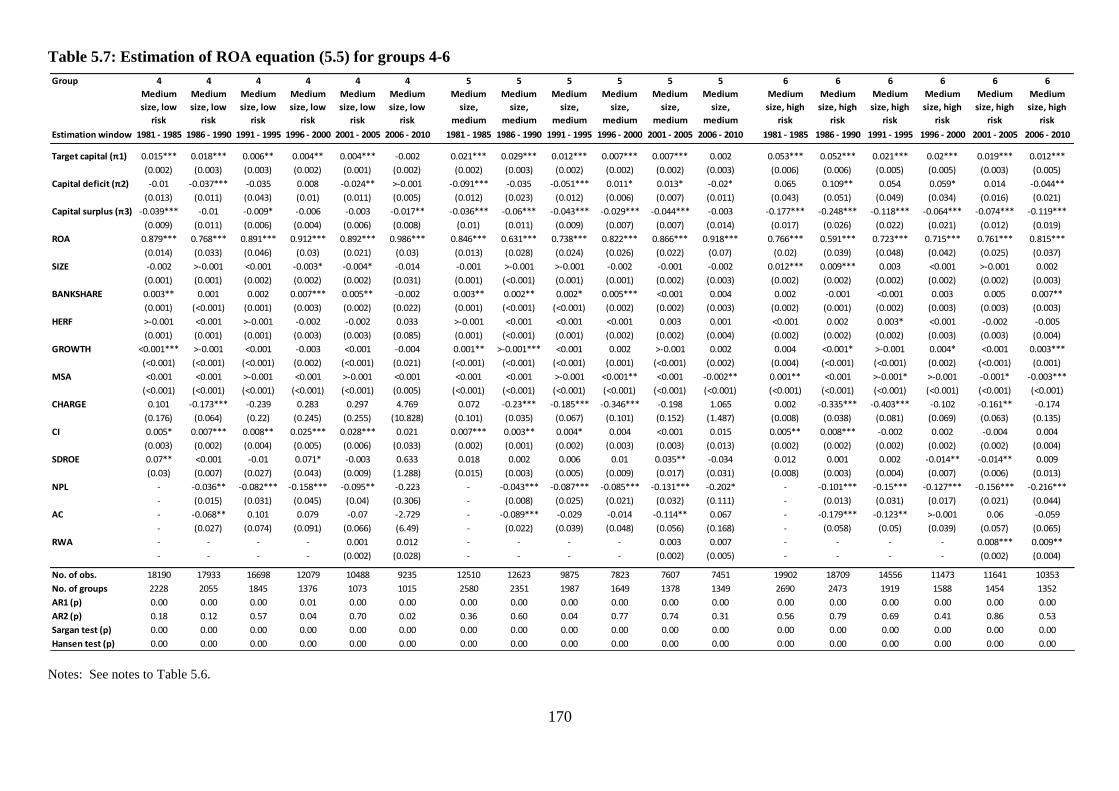
170
Table 5.7: Estimation of ROA equation (5.5) for groups 4-6
Notes: See notes to Table 5.6.
Group 4 4 4 4 4 4 5 5 5 5 5 5 6 6 6 6 6 6
Medium
size, low
risk
Medium
size, low
risk
Medium
size, low
risk
Medium
size, low
risk
Medium
size, low
risk
Medium
size, low
risk
Medium
size,
medium
risk
Medium
size,
medium
risk
Medium
size,
medium
risk
Medium
size,
medium
risk
Medium
size,
medium
risk
Medium
size,
medium
risk
Medium
size, high
risk
Medium
size, high
risk
Medium
size, high
risk
Medium
size, high
risk
Medium
size, high
risk
Medium
size, high
risk
Estimation window 1981 - 1985 1986 - 1990 1991 - 1995 1996 - 2000 2001 - 2005 2006 - 2010 1981 - 1985 1986 - 1990 1991 - 1995 1996 - 2000 2001 - 2005 2006 - 2010 1981 - 1985 1986 - 1990 1991 - 1995 1996 - 2000 2001 - 2005 2006 - 2010
Target capital (π1) 0.015*** 0.018*** 0.006** 0.004** 0.004*** -0.002 0.021*** 0.029*** 0.012*** 0.007*** 0.007*** 0.002 0.053*** 0.052*** 0.021*** 0.02*** 0.019*** 0.012***
(0.002) (0.003) (0.003) (0.002) (0.001) (0.002) (0.002) (0.003) (0.002) (0.002) (0.002) (0.003) (0.006) (0.006) (0.005) (0.005) (0.003) (0.005)
Capital deficit (π2) -0.01 -0.037*** -0.035 0.008 -0.024** >-0.001 -0.091*** -0.035 -0.051*** 0.011* 0.013* -0.02* 0.065 0.109** 0.054 0.059* 0.014 -0.044**
(0.013) (0.011) (0.043) (0.01) (0.011) (0.005) (0.012) (0.023) (0.012) (0.006) (0.007) (0.011) (0.043) (0.051) (0.049) (0.034) (0.016) (0.021)
Capital surplus (π3) -0.039*** -0.01 -0.009* -0.006 -0.003 -0.017** -0.036*** -0.06*** -0.043*** -0.029*** -0.044*** -0.003 -0.177*** -0.248*** -0.118*** -0.064*** -0.074*** -0.119***
(0.009) (0.011) (0.006) (0.004) (0.006) (0.008) (0.01) (0.011) (0.009) (0.007) (0.007) (0.014) (0.017) (0.026) (0.022) (0.021) (0.012) (0.019)
ROA 0.879*** 0.768*** 0.891*** 0.912*** 0.892*** 0.986*** 0.846*** 0.631*** 0.738*** 0.822*** 0.866*** 0.918*** 0.766*** 0.591*** 0.723*** 0.715*** 0.761*** 0.815***
(0.014) (0.033) (0.046) (0.03) (0.021) (0.03) (0.013) (0.028) (0.024) (0.026) (0.022) (0.07) (0.02) (0.039) (0.048) (0.042) (0.025) (0.037)
SIZE -0.002 >-0.001 <0.001 -0.003* -0.004* -0.014 -0.001 >-0.001 >-0.001 -0.002 -0.001 -0.002 0.012*** 0.009*** 0.003 <0.001 >-0.001 0.002
(0.001) (0.001) (0.002) (0.002) (0.002) (0.031) (0.001) (<0.001) (0.001) (0.001) (0.002) (0.003) (0.002) (0.002) (0.002) (0.002) (0.002) (0.003)
BANKSHARE 0.003** 0.001 0.002 0.007*** 0.005** -0.002 0.003** 0.002** 0.002* 0.005*** <0.001 0.004 0.002 -0.001 <0.001 0.003 0.005 0.007**
(0.001) (<0.001) (0.001) (0.003) (0.002) (0.022) (0.001) (<0.001) (<0.001) (0.002) (0.002) (0.003) (0.002) (0.001) (0.002) (0.003) (0.003) (0.003)
HERF >-0.001 <0.001 >-0.001 -0.002 -0.002 0.033 >-0.001 <0.001 <0.001 <0.001 0.003 0.001 <0.001 0.002 0.003* <0.001 -0.002 -0.005
(0.001) (0.001) (0.001) (0.003) (0.003) (0.085) (0.001) (<0.001) (0.001) (0.002) (0.002) (0.004) (0.002) (0.002) (0.002) (0.003) (0.003) (0.004)
GROWTH <0.001*** >-0.001 <0.001 -0.003 <0.001 -0.004 0.001** >-0.001*** <0.001 0.002 >-0.001 0.002 0.004 <0.001* >-0.001 0.004* <0.001 0.003***
(<0.001) (<0.001) (<0.001) (0.002) (<0.001) (0.021) (<0.001) (<0.001) (<0.001) (0.001) (<0.001) (0.002) (0.004) (<0.001) (<0.001) (0.002) (<0.001) (0.001)
MSA <0.001 <0.001 >-0.001 <0.001 >-0.001 <0.001 <0.001 <0.001 >-0.001 <0.001** <0.001 -0.002** 0.001** <0.001 >-0.001* >-0.001 -0.001* -0.003***
(<0.001) (<0.001) (<0.001) (<0.001) (<0.001) (0.005) (<0.001) (<0.001) (<0.001) (<0.001) (<0.001) (<0.001) (<0.001) (<0.001) (<0.001) (<0.001) (<0.001) (<0.001)
CHARGE 0.101 -0.173*** -0.239 0.283 0.297 4.769 0.072 -0.23*** -0.185*** -0.346*** -0.198 1.065 0.002 -0.335*** -0.403*** -0.102 -0.161** -0.174
(0.176) (0.064) (0.22) (0.245) (0.255) (10.828) (0.101) (0.035) (0.067) (0.101) (0.152) (1.487) (0.008) (0.038) (0.081) (0.069) (0.063) (0.135)
CI 0.005* 0.007*** 0.008** 0.025*** 0.028*** 0.021 0.007*** 0.003** 0.004* 0.004 <0.001 0.015 0.005** 0.008*** -0.002 0.002 -0.004 0.004
(0.003) (0.002) (0.004) (0.005) (0.006) (0.033) (0.002) (0.001) (0.002) (0.003) (0.003) (0.013) (0.002) (0.002) (0.002) (0.002) (0.002) (0.004)
SDROE 0.07** <0.001 -0.01 0.071* -0.003 0.633 0.018 0.002 0.006 0.01 0.035** -0.034 0.012 0.001 0.002 -0.014** -0.014** 0.009
(0.03) (0.007) (0.027) (0.043) (0.009) (1.288) (0.015) (0.003) (0.005) (0.009) (0.017) (0.031) (0.008) (0.003) (0.004) (0.007) (0.006) (0.013)
NPL - -0.036** -0.082*** -0.158*** -0.095** -0.223 - -0.043*** -0.087*** -0.085*** -0.131*** -0.202* - -0.101*** -0.15*** -0.127*** -0.156*** -0.216***
- (0.015) (0.031) (0.045) (0.04) (0.306) - (0.008) (0.025) (0.021) (0.032) (0.111) - (0.013) (0.031) (0.017) (0.021) (0.044)
AC - -0.068** 0.101 0.079 -0.07 -2.729 - -0.089*** -0.029 -0.014 -0.114** 0.067 - -0.179*** -0.123** >-0.001 0.06 -0.059
- (0.027) (0.074) (0.091) (0.066) (6.49) - (0.022) (0.039) (0.048) (0.056) (0.168) - (0.058) (0.05) (0.039) (0.057) (0.065)
RWA - - - - 0.001 0.012 - - - - 0.003 0.007 - - - - 0.008*** 0.009**
- - - - (0.002) (0.028) - - - - (0.002) (0.005) - - - - (0.002) (0.004)
No. of obs. 18190 17933 16698 12079 10488 9235 12510 12623 9875 7823 7607 7451 19902 18709 14556 11473 11641 10353
No. of groups 2228 2055 1845 1376 1073 1015 2580 2351 1987 1649 1378 1349 2690 2473 1919 1588 1454 1352
AR1 (p) 0.00 0.00 0.00 0.01 0.00 0.00 0.00 0.00 0.00 0.00 0.00 0.00 0.00 0.00 0.00 0.00 0.00 0.00
AR2 (p) 0.18 0.12 0.57 0.04 0.70 0.02 0.36 0.60 0.04 0.77 0.74 0.31 0.56 0.79 0.69 0.41 0.86 0.53
Sargan test (p) 0.00 0.00 0.00 0.00 0.00 0.00 0.00 0.00 0.00 0.00 0.00 0.00 0.00 0.00 0.00 0.00 0.00 0.00
Hansen test (p) 0.00 0.00 0.00 0.00 0.00 0.00 0.00 0.00 0.00 0.00 0.00 0.00 0.00 0.00 0.00 0.00 0.00 0.00

171
Table 5.8: Estimation of ROA equation (5.4) for groups 7-9
Notes: See notes to Table 5.6.
Group 7 7 7 7 7 7 8 8 8 8 8 8 9 9 9 9 9 9
Big size,
low risk
Big size,
low risk
Big size,
low risk
Big size,
low risk
Big size,
low risk
Big size,
low risk
Big size,
medium
risk
Big size,
medium
risk
Big size,
medium
risk
Big size,
medium
risk
Big size,
medium
risk
Big size,
medium
risk
Big size,
high risk
Big size,
high risk
Big size,
high risk
Big size,
high risk
Big size,
high risk
Big size,
high risk
Estimation window 1981 - 1985 1986 - 1990 1991 - 1995 1996 - 2000 2001 - 2005 2006 - 2010 1981 - 1985 1986 - 1990 1991 - 1995 1996 - 2000 2001 - 2005 2006 - 2010 1981 - 1985 1986 - 1990 1991 - 1995 1996 - 2000 2001 - 2005 2006 - 2010
Target capital (π1) 0.007*** 0.013*** 0.003*** 0.003** -0.004*** 0.001 0.007*** 0.013*** 0.01*** 0.005* 0.006*** 0.008*** 0.032*** 0.052*** 0.039*** 0.027*** 0.011*** 0.006
(0.001) (0.002) (0.001) (0.001) (0.001) (0.002) (0.001) (0.002) (0.003) (0.003) (0.001) (0.003) (0.004) (0.006) (0.006) (0.005) (0.003) (0.005)
Capital deficit (π2) -0.024*** 0.01** -0.011 0.005 -0.017*** 0.009** -0.047*** -0.008 0.023 0.009 0.015*** -0.009 0.028 0.072*** 0.018 0.016** 0.009 -0.01
(0.008) (0.004) (0.011) (0.004) (0.005) (0.005) (0.01) (0.007) (0.016) (0.008) (0.005) (0.006) (0.033) (0.026) (0.012) (0.007) (0.009) (0.011)
Capital surplus (π3) -0.04*** -0.013*** -0.016*** -0.011** -0.033*** -0.036* -0.031*** -0.035*** -0.028 -0.013*** -0.029*** -0.031*** -0.183*** -0.202*** -0.145*** -0.02 -0.009 -0.063***
(0.008) (0.003) (0.006) (0.005) (0.011) (0.021) (0.007) (0.006) (0.025) (0.004) (0.005) (0.009) (0.019) (0.019) (0.02) (0.015) (0.008) (0.016)
ROA 0.956*** 0.863*** 0.912*** 0.903*** 1.056*** 0.939*** 0.937*** 0.821*** 0.879*** 0.938*** 0.877*** 0.848*** 0.828*** 0.551*** 0.687*** 0.725*** 0.858*** 0.859***
(0.008) (0.017) (0.016) (0.023) (0.039) (0.006) (0.007) (0.022) (0.039) (0.05) (0.018) (0.02) (0.014) (0.03) (0.043) (0.026) (0.027) (0.031)
SIZE -0.018*** -0.003* -0.004 -0.003 0.006 -0.014* <0.001 <0.001 <0.001 -0.002 0.001 >-0.001 0.001 0.004** 0.004** 0.006*** <0.001 >-0.001
(0.004) (0.001) (0.003) (0.002) (0.008) (0.007) (0.002) (0.001) (0.002) (0.003) (0.002) (0.002) (0.003) (0.002) (0.002) (0.002) (0.003) (0.004)
BANKSHARE -0.001 0.002 <0.001 0.003 0.008** 0.014*** 0.002 0.002* 0.003** 0.005** 0.01*** 0.008*** 0.002 0.001 0.008*** 0.006*** 0.003 >-0.001
(0.003) (0.001) (0.002) (0.004) (0.004) (0.005) (0.002) (<0.001) (0.001) (0.002) (0.002) (0.003) (0.002) (0.001) (0.001) (0.002) (0.004) (0.006)
HERF 0.003 >-0.001 0.003 0.002 -0.008 -0.009 0.001 -0.001 -0.003 <0.001 -0.008*** <0.001 -0.004* -0.003 -0.003** >-0.001 0.009 0.004
(0.003) (0.001) (0.002) (0.004) (0.006) (0.007) (0.002) (0.001) (0.002) (0.004) (0.003) (0.003) (0.002) (0.002) (0.002) (0.003) (0.009) (0.007)
GROWTH 0.004 >-0.001*** 0.001 0.002** 0.005 -0.002 <0.001 >-0.001** >-0.001 <0.001 0.002 <0.001 <0.001 <0.001 <0.001 0.004* 0.005* 0.002
(0.003) (<0.001) (<0.001) (<0.001) (0.005) (0.003) (<0.001) (<0.001) (<0.001) (0.001) (0.001) (<0.001) (<0.001) (<0.001) (<0.001) (0.002) (0.003) (0.003)
MSA <0.001 <0.001 <0.001 >-0.001 >-0.001 <0.001 0.001*** <0.001 <0.001 <0.001* <0.001 >-0.001 0.001* >-0.001 <0.001 <0.001 <0.001 -0.003
(<0.001) (<0.001) (<0.001) (<0.001) (0.001) (0.001) (<0.001) (<0.001) (<0.001) (<0.001) (<0.001) (<0.001) (<0.001) (<0.001) (<0.001) (<0.001) (0.001) (0.002)
CHARGE 1.752*** -0.181* -0.198 0.285 -0.538 0.96** 0.473** -0.066 0.204* -0.175 0.134 -0.057 <0.001 -0.264*** -0.163** 0.041 0.222*** 0.077
(0.518) (0.098) (0.165) (0.261) (0.525) (0.437) (0.203) (0.083) (0.122) (0.314) (0.171) (0.154) (0.014) (0.036) (0.067) (0.074) (0.063) (0.103)
CI 0.04*** 0.004* 0.007 0.018*** 0.02* 0.014 0.008*** 0.004*** 0.009*** 0.01 >-0.001 0.01** 0.006*** 0.004** >-0.001 -0.003 -0.002 0.021
(0.01) (0.002) (0.004) (0.007) (0.011) (0.022) (0.003) (0.001) (0.003) (0.007) (0.003) (0.004) (0.002) (0.002) (0.002) (0.002) (0.007) (0.013)
SDROE 0.051 <0.001 -0.009 0.089*** -0.015 0.166* 0.059** -0.002 0.026** 0.081 0.061*** 0.047*** 0.023** -0.005* -0.005* -0.014*** 0.048 0.048
(0.038) (0.009) (0.027) (0.026) (0.049) (0.089) (0.024) (0.006) (0.012) (0.087) (0.021) (0.014) (0.01) (0.003) (0.003) (0.005) (0.034) (0.05)
NPL - -0.08*** -0.066* -0.002 -0.044 -0.24*** - -0.103*** -0.054** -0.135 -0.044 -0.13*** - -0.132*** -0.181*** -0.122*** -0.329*** -0.353***
- (0.025) (0.034) (0.046) (0.098) (0.089) - (0.015) (0.026) (0.108) (0.036) (0.029) - (0.012) (0.019) (0.045) (0.054) (0.106)
AC - 0.14*** 0.068* 0.091*** 0.357** -0.083 - -0.022 <0.001 0.023 0.037 0.051* - -0.024 0.057** 0.064** 0.144* 0.084*
- (0.031) (0.038) (0.024) (0.146) (0.067) - (0.029) (0.044) (0.042) (0.058) (0.03) - (0.03) (0.028) (0.029) (0.084) (0.051)
RWA - - - - -0.011* 0.011 - - - - 0.009*** 0.005** - - - - 0.01*** 0.012*
- - - - (0.005) (0.007) - - - - (0.002) (0.002) - - - - (0.004) (0.007)
No. of obs. 16067 18494 10789 10445 11421 8266 17609 17972 13607 9799 9288 8370 21488 18211 22131 16549 14507 14476
No. of groups 2070 1969 1258 1125 1025 863 2882 2805 2151 1644 1417 1398 2523 2270 2253 1965 1491 1592
AR1 (p) 0.00 0.00 0.00 0.00 0.08 0.17 0.00 0.00 0.00 0.01 0.00 0.00 0.00 0.00 0.00 0.00 0.01 0.00
AR2 (p) 0.08 0.20 0.83 0.31 0.77 0.63 0.04 0.62 0.98 0.24 0.52 0.28 0.87 0.83 0.78 0.79 0.42 0.28
Sargan test (p) 0.00 0.00 0.00 0.00 0.00 0.05 0.00 0.00 0.00 0.00 0.00 0.00 0.00 0.00 0.00 0.00 0.00 0.00
Hansen test (p) 0.00 0.00 0.00 0.00 0.00 0.00 0.00 0.00 0.00 0.00 0.00 0.00 0.00 0.00 0.00 0.00 0.00 0.00

172
Figure 5.6: Coefficients on capital variables in regression of ROA
Notes: The charts show the total coefficients on 𝑘𝑖𝑡∗ (𝜋1), 𝑘𝑖𝑡
𝑆𝑢𝑟𝑝𝑙𝑢𝑠(𝜋3) and 𝑘𝑖𝑡
𝐷𝑒𝑓𝑖𝑐𝑖𝑡(𝜋2) from estimation of (5.5) on quarterly data and 5-year estimation windows. The return on assets (ROA)
is regressed on four lags of itself, four lags of the capital variables, and lags of the following control variables: the bank‘s share of local deposit markets (BANKSHARE), the Herfindahl index
for the bank‘s local deposit markets (HERF), annual growth of a bank‘s local deposit markets (GROWTH), the proportion of a bank‘s deposits in urban markets (MSA), the ratio of charge-offs
to total assets (CHARGE), the ratio of commercial and industrial loans to total assets (C&I), the standard deviation of ROE (SDROE), the ratio of non-performing loans to total assets (NPL,
after 1984), the ratio of risk-weighted assets to total assets (RW, after 1996), the size rank index based on total assets (SIZE) and the ratio of operating costs to total assets (AC, after 1984).
Bank and time fixed effects are included. Estimated using two-step system GMM. Bands show two standard errors (~95%).
-0.1
-0.05
0
0.05
0.1
0.15
Group 1: Small size, low risk
Target capital ratio (π1)
-0.4
-0.2
0
0.2
0.4
0.6
0.8 Capital deficit (π2)
-0.02
0
0.02
0.04
0.06
0.08
0.1
Group 2: Small size, medium risk
Target capital ratio (π1)
-0.4
-0.2
0
0.2
0.4
0.6
0.8
1
1.2 Capital deficit (π2)
0
0.02
0.04
0.06
0.08
0.1
0.12
Group 3: Small size, high risk
Target capital ratio (π1)
-0.1
0
0.1
0.2
0.3
0.4 Capital deficit (π2)
-0.8
-0.6
-0.4
-0.2
0
0.2
0.4
0.6Capital surplus (π3)
-0.4
-0.35
-0.3
-0.25
-0.2
-0.15
-0.1
-0.05
0
0.05 Capital surplus (π3)
-0.3
-0.25
-0.2
-0.15
-0.1
-0.05
0Capital surplus (π3)

173
Figure 5.6: Coefficients on capital variables in regression of ROA (continued)
Notes: The charts show the total coefficients on 𝑘𝑖𝑡∗ (𝜋1), 𝑘𝑖𝑡
𝑆𝑢𝑟𝑝𝑙𝑢𝑠(𝜋3) and 𝑘𝑖𝑡
𝐷𝑒𝑓𝑖𝑐𝑖𝑡(𝜋2) from estimation of (5.5) on quarterly data and 5-year estimation windows. The return on assets (ROA)
is regressed on four lags of itself, four lags of the capital variables, and lags of the following control variables: the bank‘s share of local deposit markets (BANKSHARE), the Herfindahl index
for the bank‘s local deposit markets (HERF), annual growth of a bank‘s local deposit markets (GROWTH), the proportion of a bank‘s deposits in urban markets (MSA), the ratio of charge-offs
to total assets (CHARGE), the ratio of commercial and industrial loans to total assets (C&I), the standard deviation of ROE (SDROE), the ratio of non-performing loans to total assets (NPL,
after 1984), the ratio of risk-weighted assets to total assets (RW, after 1996), the size rank index based on total assets (SIZE) and the ratio of operating costs to total assets (AC, after 1984).
Bank and time fixed effects are included. Estimated using two-step system GMM. Bands show two standard errors (~95%).
-0.01
0
0.01
0.02
0.03
Group 4: Medium size, low risk
Target capital ratio (π1)
-0.15
-0.1
-0.05
0
0.05
0.1 Capital deficit (π2)
-0.1
-0.05
0
0.05 Capital surplus (π3)
-0.01
0
0.01
0.02
0.03
0.04
0.05
Group 5: Medium size, medium risk
Target capital ratio (π1)
-0.15
-0.1
-0.05
0
0.05 Capital deficit (π2)
-0.1
-0.05
0
0.05 Capital surplus (π3)
-0.02
0
0.02
0.04
0.06
0.08
0.1
0.12
Group 6: Medium size, high risk
Target capital ratio (π1)
-0.2
-0.1
0
0.1
0.2
0.3 Capital deficit (π2)
-0.4
-0.3
-0.2
-0.1
0Capital surplus (π3)

174
Figure 5.6: Coefficients on capital variables in regression of ROA (continued)
Notes: The charts show the total coefficients on 𝑘𝑖𝑡∗ (𝜋1), 𝑘𝑖𝑡
𝑆𝑢𝑟𝑝𝑙𝑢𝑠(𝜋3) and 𝑘𝑖𝑡
𝐷𝑒𝑓𝑖𝑐𝑖𝑡(𝜋2) from estimation of (5.5) on quarterly data and 5-year estimation windows. The return on assets (ROA)
is regressed on four lags of itself, four lags of the capital variables, and lags of the following control variables: the bank‘s share of local deposit markets (BANKSHARE), the Herfindahl index
for the bank‘s local deposit markets (HERF), annual growth of a bank‘s local deposit markets (GROWTH), the proportion of a bank‘s deposits in urban markets (MSA), the ratio of charge-offs
to total assets (CHARGE), the ratio of commercial and industrial loans to total assets (C&I), the standard deviation of ROE (SDROE), the ratio of non-performing loans to total assets (NPL,
after 1984), the ratio of risk-weighted assets to total assets (RW, after 1996), the size rank index based on total assets (SIZE) and the ratio of operating costs to total assets (AC, after 1984).
Bank and time fixed effects are included. Estimated using two-step system GMM. Bands show two standard errors (~95%).
-0.02
-0.01
0
0.01
0.02
Group 7: Big size, low risk
Target capital ratio (π1)
-0.1
-0.05
0
0.05 Capital deficit (π2)
-0.1
-0.05
0
0.05 Capital surplus (π3)
-0.005
0
0.005
0.01
0.015
0.02
0.025
Group 8: Big size, medium risk
Target capital ratio (π1)
-0.1
-0.05
0
0.05
0.1 Capital deficit (π2)
-0.15
-0.1
-0.05
0
0.05 Capital surplus (π3)
-0.02
0
0.02
0.04
0.06
0.08
0.1
Group 9: Big size, high risk
Target capital ratio (π1)
-0.1
0
0.1
0.2 Capital deficit (π2)
-0.3
-0.2
-0.1
0
0.1Capital surplus (π3)
175
5.4.3 Robustness tests
a) Multicollinearity amongst the portfolio risk variables
In the analysis above we have included a number of control variables for the level of portfolio
risk at each bank over time. These are the standard deviation of ROE (SDROE), the ratio of
commercial and industrial loans to total loans (C&I), the ratio of charge-offs to total loans
(CHARGE), the ratio of non-performing loans to total loans (NPL), and the ratio of risk-
weighted assets to total assets (RW). Our intention in including a wide variety of risk
measures is to capture as many different dimensions of the risk that a bank is exposed to from
the perspective of its investors. However, one possible criticism of this approach is that the
risk measures may overlap with each other to an unhelpful extent resulting in
multicollinearity. Multicollinearity causes problems with interpretation of the regression
results since it can result in highly unstable coefficient estimates and very large standards
errors of the coefficient estimates (see, e.g., Greene, 2008). Therefore we wish to test for the
presence of multicollinearity of our risk measures. We do this using the ―Klein rule of
thumb‖ method. In this method, a set of auxiliary models are estimated regressing each of
the risk measures on the other risk measures. If the R-squared of the auxiliary regressions is
higher than the R-squared of the main regression, then this is a sign that multicollinearity may
be a problem.
We performed this test for six selected windows in our sample, using all banks in the dataset.
For each time window τ, we first estimate our main model for the return on assets given by
equation (5.5) above. Preserving the estimation sample from estimating the main model, we
then estimate auxiliary regressions as follows:
𝐶𝐻𝐴𝑅𝐺𝐸𝑖𝑡 = 𝛼𝜏 + 𝜃𝑡 + 𝜐𝑖 + 𝛽1𝜏𝑁𝑃𝐿𝑖𝑡 + 𝛽2𝜏𝐶&𝐼𝑖𝑡 + 𝛽3𝜏𝑆𝐷𝑅𝑂𝐸𝑖𝑡 + 𝛽4𝜏𝑅𝑊𝑖𝑡 + 𝑒𝑖𝑡
𝑁𝑃𝐿𝑖𝑡 = 𝛼𝜏 + 𝜃𝑡 + 𝜐𝑖 + 𝛽5𝜏𝐶𝐻𝐴𝑅𝐺𝐸𝑖𝑡 + 𝛽6𝜏𝐶&𝐼𝑖𝑡 + 𝛽7𝜏𝑆𝐷𝑅𝑂𝐸𝑖𝑡 + 𝛽8𝜏𝑅𝑊𝑖𝑡 + 𝑒𝑖𝑡
and so on for the other three risk variables, SDROE, RW and C&I. Only those risk measures
that are available are included in the analysis for each window, as in the analysis above. The
full regression and the auxiliary regressions are estimated using fixed effects.
The results are shown in Table 5.9 below. Since the R-squared for all of the auxiliary
regressions is well below the R-squared of the full regression, we conclude that

176
multicollinearity amongst the risk variables is not a problem for the models presented in this
chapter.
Table 5.9: Klein tests for multicollinearity amongst risk variables
b) Re-estimating models using fixed effects estimator
As we noted above, using the standard fixed effects estimator for dynamic panels may result
in biased estimates due to the inclusion of a lagged dependent variable. This drove our
choice of the GMM estimator for our improved specification in section 5.4.2 above.
However, as we have shown, the diagnostic tests do not support the key assumption that the
instruments used for the endogenous variables are exogenous. Furthermore, as other studies
have shown, the lagged dependent variable bias associated with fixed effects is declining in
the number of time periods (Judson and Owen, 1999; Flannery and Hankins, 2012),
suggesting that in our ROA models where there are 20 quarterly time periods (5 years * 4
quarters), the economic significance of the bias may be relatively small, although the bias
may be more of a problem for the target capital ratio models where there are only 5 annual
time periods. Furthermore, since we are primarily interested in the change rather than the
level of the parameters of interest (i.e., the long-run coefficient of CAR in the ROA equation)
the bias may not prevent us from drawing conclusions from the fixed effects estimates.
Therefore, overall it is not clear whether the GMM estimates should be preferred to the fixed
effects estimates for inferring the economic effects of interest. A better approach may be to
draw inferences from a comparison of the GMM and fixed effects estimates.
In this section we therefore provide a complete set of results for both the target capital ratio
equation (5.2) and the ROA equation (5.5) re-estimated using the fixed effects estimator.
1980 - 1984 1985 - 1989 1990 - 1994 1995 - 1999 2000 - 2004 2000 - 2004 2005 - 2009
Full specification 0.78 0.92 0.82 0.64 0.60 0.60 0.97
Regression of risk variables
only with dependent variable:
CHARGE 0.04 0.37 0.10 0.14 0.07 0.07 0.24
C&I 0.00 0.00 0.01 0.00 0.20 0.20 0.17
SDROE 0.03 0.23 0.04 0.11 0.06 0.06 0.24
NPL 0.00 0.23 0.11 0.11 0.11 0.11 0.23
RW 0.00 0.00 0.00 0.00 0.20 0.20 0.16

177
First, we examine the results of estimating the target capital ratio equation (5.2) using fixed
effects, which are shown in Table 5.10, Table 5.11 and Table 5.12. As above, we also show
the target capital ratio and actual capital ratio, together with capital buffers at the 10th
, 25th
,
75th
and 90th
percentiles, in Figure 5.5. Note that by the nature of the lagged dependent
variable bias we expect that the coefficient on the lagged dependent variable is biased
upwards and the coefficients on the other explanatory variables are downward biased, so
overall the effects on the long-run coefficients are ambiguous in sign. In the fixed effects
models, the main explanatory variables continue to be SIZE (negative), BANKSHARE
(positive), and ROA (positive), and C&I (negative). In general, the overall R2 of these
regressions are above 0.5, indicating a relatively good model fit. Examining the actual and
target capital ratios in Figure 5.5, we see that the actual capital ratio tracks the target capital
ratio fairly closely with few persistent deviations on average (with the exception of small
size, low risk group for which the median target capital ratio is below the median actual
capital ratio throughout the 2000s) but a good range of buffers above and below the target
capital ratio.

178
Table 5.10: Estimation of target capital ratio equation (5.2), using fixed effects estimator, groups 1-3
Notes: The table shows the long run coefficients derived from estimation of reduced form Equation (5.2) for three groups: 1 (small, low risk), 2 (small, medium risk) and 3
(small, high risk). Table shows 7 windows per group selected from the 30 that are estimated. The capital asset ratio (k) is regressed on one lag of itself and lags of the
following control variables: the bank‘s share of local deposit markets (BANKSHARE), the Herfindahl index for the bank‘s local deposit markets (HERF), annual growth of a
bank‘s local deposit markets (GROWTH), the proportion of a bank‘s deposits in urban markets (MSA), the ratio of charge-offs to total assets (CHARGE), the ratio of
commercial and industrial loans to total assets (C&I), the standard deviation of ROE (SDROE), the ratio of non-performing loans to total assets (NPL), the ratio of risk-
weighted assets to total assets (RW), our size index based on total assets (SIZE) and the ratio of operating costs to total assets (AC). Bank fixed effects and time effects are
included. Estimated using fixed effects (i.e. least squares dummy variable estimator).
Group
Start year 1977 1981 1986 1991 1996 2001 2006 1977 1981 1986 1991 1996 2001 2006 1977 1981 1986 1991 1996 2001 2006
End year 1980 1985 1990 1995 2000 2005 2010 1980 1985 1990 1995 2000 2005 2010 1980 1985 1990 1995 2000 2005 2010
SIZE -0.203*** -0.155*** -0.12*** -0.144*** -0.16*** -0.158*** -0.248*** -0.165*** -0.142*** -0.107*** -0.12*** -0.101*** -0.088*** -0.133*** -0.085*** -0.063*** 0.009 -0.052*** -0.06*** -0.079*** -0.089***
(0.007) (0.008) (0.014) (0.01) (0.017) (0.016) (0.017) (0.007) (0.006) (0.006) (0.01) (0.01) (0.008) (0.013) (0.007) (0.006) (0.007) (0.007) (0.011) (0.012) (0.015)
ROA 0.847*** 0.438*** 0.029 -0.058 0.169*** 0.332*** 0.596*** 0.281*** 0.318*** 0.323*** -0.414*** 0.157* 0.561*** 0.698*** 0.244*** 0.291*** 0.368*** 0.308*** 0.147** 0.797*** 0.232***
(0.082) (0.067) (0.028) (0.039) (0.052) (0.025) (0.063) (0.048) (0.041) (0.04) (0.057) (0.091) (0.079) (0.094) (0.03) (0.025) (0.028) (0.036) (0.061) (0.074) (0.07)
BANKSHARE 0.043** 0.031** 0.048*** 0.009 0.187*** 0.112*** 0.095*** 0.034** 0.033** 0.014 0.014* 0.052* 0.031 0.199*** -0.021 -0.003 0.012 0.023* 0.022 -0.014 -0.004
(0.019) (0.012) (0.015) (0.012) (0.049) (0.041) (0.034) (0.015) (0.013) (0.01) (0.008) (0.029) (0.023) (0.033) (0.018) (0.013) (0.02) (0.012) (0.029) (0.033) (0.049)
HERF -0.009 -0.019 0.023** -0.011 -0.053 0.08*** -0.022 -0.016 -0.01 0.002 -0.018*** 0.005 -0.037** 0.06*** 0.023 >-0.001 -0.028** 0.008 -0.011 -0.052** 0.037
(0.016) (0.012) (0.011) (0.009) (0.034) (0.025) (0.028) (0.011) (0.009) (0.007) (0.007) (0.024) (0.015) (0.022) (0.015) (0.011) (0.013) (0.009) (0.025) (0.025) (0.039)
GROWTH -0.005* -0.003 >-0.001 -0.008*** 0.037*** -0.008* 0.023*** 0.003 0.002 >-0.001 0.004** 0.009 0.004* -0.015** -0.001 <0.001 >-0.001 <0.001** 0.008 -0.002 -0.002
(0.003) (0.002) (0.002) (0.003) (0.011) (0.005) (0.008) (0.002) (0.002) (<0.001) (0.002) (0.008) (0.003) (0.006) (0.003) (0.001) (0.003) (<0.001) (0.008) (0.003) (0.004)
MSA -0.005 -0.004 -0.008 0.003 -0.006 0.101*** 0.073*** <0.001 <0.001 <0.001 -0.015*** 0.012 0.021 -0.007 0.002 <0.001 -0.017* <0.001 -0.04*** -0.035*** -0.004
(0.006) (0.003) (0.011) (0.004) (0.02) (0.029) (0.025) (0.003) (0.003) (0.008) (0.003) (0.009) (0.016) (0.014) (0.005) (0.003) (0.01) (0.004) (0.011) (0.013) (0.019)
CHARGE -0.139 -0.028 -0.213 0.458** -2.25*** -0.507 0.509 -0.143 -0.071 -0.038 0.886*** -0.847*** 0.716*** 0.004 -0.091 -0.019 0.194*** 0.247*** 0.259* 0.753*** 0.417**
(0.251) (0.3) (0.163) (0.223) (0.552) (0.529) (0.58) (0.094) (0.106) (0.055) (0.118) (0.241) (0.159) (0.208) (0.064) (0.048) (0.053) (0.072) (0.146) (0.166) (0.169)
C&I -0.056*** -0.011 -0.133*** -0.058*** -0.085** 0.009 -0.059* 0.009 -0.013* 0.006 -0.034*** -0.021 -0.031** -0.045** -0.004 -0.02*** -0.009 -0.004 -0.04*** -0.041*** >-0.001
(0.017) (0.014) (0.017) (0.021) (0.036) (0.039) (0.035) (0.008) (0.007) (0.008) (0.011) (0.016) (0.013) (0.018) (0.006) (0.007) (0.009) (0.01) (0.015) (0.015) (0.019)
SDROE -0.064* -0.016 -0.011 -0.044*** 0.07*** 0.048*** -0.146*** 0.038* 0.024** -0.011*** 0.006 -0.037*** 0.021 0.056** 0.078*** 0.045*** 0.03*** 0.025*** 0.026** 0.075*** 0.032**
(0.034) (0.021) (0.01) (0.014) (0.016) (0.018) (0.034) (0.02) (0.011) (0.004) (0.004) (0.012) (0.019) (0.022) (0.008) (0.004) (0.004) (0.004) (0.011) (0.019) (0.015)
NPL - - 0.036 -0.207* 0.116 -0.112 -0.065 - - -0.013 -0.202*** -0.047 -0.209*** -0.061 - - -0.304*** -0.009 -0.083* -0.127** -0.265***
- - (0.086) (0.108) (0.16) (0.173) (0.125) - - (0.026) (0.043) (0.062) (0.057) (0.055) - - (0.024) (0.029) (0.044) (0.051) (0.043)
OPEFF - - 2.842*** -0.157*** -0.118* -0.085*** 0.875*** - - -0.408*** 0.328*** -0.194 -0.687*** -0.079 - - -0.131 -0.041 1.321*** -0.35** -0.011
- - (0.138) (0.033) (0.071) (0.015) (0.186) - - (0.101) (0.017) (0.166) (0.162) (0.085) - - (0.12) (0.086) (0.114) (0.178) (0.128)
RW - - - - - 0.02* -0.029** - - - - - -0.008 -0.018** - - - - - -0.045*** -0.016
- - - - - (0.011) (0.013) - - - - - (0.006) (0.009) - - - - - (0.01) (0.014)
Number of obs. 6181 6891 6631 7366 5333 4879 4926 5979 6993 6403 5766 4565 4128 3645 6303 8102 7702 5141 4146 3582 2698
Number of banks 2527 2584 2383 2602 1891 1646 1560 3043 3362 3022 2784 2139 1877 1662 2696 3201 2990 2100 1699 1437 1181
R2 (overall) 0.67 0.77 0.25 0.79 0.68 0.74 0.60 0.49 0.62 0.61 0.22 0.65 0.69 0.29 0.59 0.67 0.66 0.70 0.34 0.40 0.63
R2 (between) 0.65 0.77 0.25 0.80 0.63 0.72 0.59 0.52 0.65 0.63 0.21 0.62 0.68 0.32 0.64 0.72 0.73 0.75 0.39 0.43 0.61
R2 (within) 0.57 0.46 0.27 0.39 0.23 0.34 0.34 0.55 0.54 0.35 0.31 0.37 0.43 0.36 0.40 0.45 0.38 0.37 0.26 0.27 0.50
Group 1: SMALL SIZE & LOW RISK Group 2: SMALL SIZE & MEDIUM RISK Group 3: SMALL SIZE & HIGH RISK

179
Table 5.11: Estimation of target capital ratio equation (5.2), using fixed effects estimator, groups 4-6
Notes: The table shows the long run coefficients derived from estimation of reduced form Equation (5.2) for three groups: 4 (medium size, low risk), 5 (medium size,
medium risk) and 6 (medium size, high risk). Table shows 7 windows per group selected from the 30 that are estimated. The capital asset ratio (k) is regressed on one lag of
itself and lags of the following control variables: the bank‘s share of local deposit markets (BANKSHARE), the Herfindahl index for the bank‘s local deposit markets
(HERF), annual growth of a bank‘s local deposit markets (GROWTH), the proportion of a bank‘s deposits in urban markets (MSA), the ratio of charge-offs to total assets
(CHARGE), the ratio of commercial and industrial loans to total assets (C&I), the standard deviation of ROE (SDROE), the ratio of non-performing loans to total assets
(NPL), the ratio of risk-weighted assets to total assets (RW), our size index based on total assets (SIZE) and the ratio of operating costs to total assets (AC). Bank fixed
effects and time effects are included. Estimated using fixed effects (i.e. least squares dummy variable estimator).
Group no.
Start year 1977 1981 1986 1991 1996 2001 2006 1977 1981 1986 1991 1996 2001 2006 1977 1981 1986 1991 1996 2001 2006
End year 1980 1985 1990 1995 2000 2005 2010 1980 1985 1990 1995 2000 2005 2010 1980 1985 1990 1995 2000 2005 2010
SIZE -0.11*** -0.083*** -0.063*** -0.077*** -0.135*** -0.089*** -0.074*** -0.08*** -0.07*** -0.075*** -0.069*** -0.052*** -0.029*** -0.067*** -0.064*** -0.028*** 0.017*** -0.059*** -0.033*** -0.026*** -0.071***
(0.003) (0.004) (0.003) (0.004) (0.006) (0.007) (0.007) (0.003) (0.003) (0.003) (0.003) (0.005) (0.005) (0.006) (0.003) (0.003) (0.004) (0.005) (0.005) (0.004) (0.008)
ROA 0.535*** 0.51*** 0.635*** 0.557*** 0.333*** 0.576*** 0.88*** 0.421*** 0.494*** 0.427*** 0.466*** 0.162 0.523*** 0.367*** 0.461*** 0.37*** 0.275*** 0.312*** 0.161*** 0.291*** 0.847***
(0.068) (0.045) (0.061) (0.069) (0.098) (0.08) (0.125) (0.045) (0.039) (0.038) (0.05) (0.116) (0.076) (0.063) (0.03) (0.022) (0.028) (0.037) (0.045) (0.04) (0.058)
BANKSHARE 0.014** 0.006 0.021*** 0.017*** 0.048*** 0.027 0.1*** 0.023*** 0.017*** 0.014*** 0.005 0.048** -0.003 0.058*** 0.02** 0.02*** 0.002 0.012 0.039** 0.009 -0.029
(0.007) (0.005) (0.005) (0.004) (0.016) (0.018) (0.024) (0.006) (0.005) (0.004) (0.004) (0.019) (0.014) (0.015) (0.009) (0.007) (0.008) (0.008) (0.016) (0.012) (0.024)
HERF -0.008 0.003 -0.004 -0.004 0.021 0.004 -0.075*** -0.008 -0.014** -0.001 0.02*** -0.039** 0.028** -0.024* -0.014 0.004 -0.007 -0.004 0.002 0.012 0.026
(0.008) (0.005) (0.005) (0.005) (0.014) (0.015) (0.024) (0.008) (0.006) (0.005) (0.005) (0.019) (0.013) (0.015) (0.01) (0.009) (0.009) (0.007) (0.015) (0.01) (0.019)
GROWTH 0.003** -0.002** <0.001 <0.001 >-0.001 <0.001 -0.001 <0.001 0.002 >-0.001 >-0.001 0.008 >-0.001 0.002 0.003* 0.002 >-0.001 0.003* 0.005 -0.002 >-0.001
(0.001) (<0.001) (<0.001) (0.001) (0.004) (0.003) (0.003) (0.001) (0.002) (<0.001) (<0.001) (0.006) (0.002) (0.002) (0.002) (0.001) (<0.001) (0.002) (0.004) (0.002) (0.002)
MSA 0.005** 0.002 -0.001 0.006*** 0.01 0.005 0.061*** -0.002 >-0.001 0.006 0.004* 0.002 0.011 0.002 <0.001 0.003 0.003 -0.002 0.013 0.009 0.019
(0.003) (0.001) (0.003) (0.002) (0.012) (0.02) (0.022) (0.003) (0.002) (0.003) (0.002) (0.01) (0.01) (0.007) (0.004) (0.002) (0.009) (0.003) (0.008) (0.007) (0.014)
CHARGE -0.138 0.064 0.42*** 0.589*** -0.658** 0.344 -0.943*** -0.011 0.023 0.142** 0.361*** 0.564* 0.024 -0.306 0.138*** 0.003 0.069 0.302*** 0.28*** 0.269*** 0.082
(0.242) (0.067) (0.109) (0.171) (0.307) (0.372) (0.341) (0.019) (0.028) (0.057) (0.102) (0.289) (0.231) (0.204) (0.052) (0.007) (0.054) (0.07) (0.105) (0.076) (0.14)
C&I 0.014 -0.009 -0.008 <0.001 -0.009 -0.05*** -0.01 0.005 -0.007 0.004 -0.006 -0.04*** -0.008 0.011 -0.006 -0.02*** -0.009 -0.037*** -0.034*** -0.02*** -0.017
(0.009) (0.006) (0.007) (0.009) (0.014) (0.017) (0.025) (0.005) (0.005) (0.004) (0.007) (0.014) (0.011) (0.011) (0.005) (0.004) (0.007) (0.008) (0.008) (0.007) (0.012)
SDROE 0.06** <0.001 -0.005 -0.025** -0.004 -0.006 0.057 0.01 -0.003 0.007* -0.002 0.036* -0.015 0.037** 0.034*** 0.02*** 0.008** 0.013*** 0.008 0.029*** 0.051***
(0.026) (0.013) (0.013) (0.011) (0.021) (0.028) (0.042) (0.015) (0.008) (0.004) (0.006) (0.02) (0.021) (0.016) (0.006) (0.004) (0.004) (0.004) (0.007) (0.009) (0.016)
NPL - - -0.024 0.049 -0.107 0.118 -0.019 - - -0.037* -0.159*** 0.219*** 0.069 -0.095*** - - -0.267*** -0.151*** -0.025 0.079** -0.292***
- - (0.043) (0.06) (0.079) (0.099) (0.103) - - (0.021) (0.034) (0.079) (0.069) (0.037) - - (0.02) (0.023) (0.035) (0.032) (0.028)
OPEFF - - -0.825*** -0.611*** 0.753*** 0.675*** -0.218*** - - -0.79*** -0.813*** -1.835*** -1.033*** -0.337*** - - -0.312*** 0.708*** 0.117 -0.155*** 0.308***
- - (0.057) (0.07) (0.13) (0.13) (0.078) - - (0.098) (0.106) (0.222) (0.139) (0.11) - - (0.109) (0.082) (0.081) (0.053) (0.106)
RW - - - - - -0.013** -0.019* - - - - - -0.008 -0.027*** - - - - - -0.009* -0.063***
- - - - - (0.006) (0.01) - - - - - (0.006) (0.006) - - - - - (0.005) (0.009)
Number of obs. 6186 7409 7139 6279 4786 3917 3535 6697 8130 7298 6365 5294 4588 4342 6679 8408 7544 5984 5038 4792 4214
Number of banks 2680 2935 2723 2389 1778 1427 1312 3423 3923 3496 3011 2442 2109 1967 2909 3464 3142 2482 2125 1870 1718
R2 (overall) 0.48 0.58 0.72 0.57 0.39 0.43 0.73 0.52 0.64 0.61 0.59 0.65 0.67 0.52 0.50 0.67 0.68 0.50 0.70 0.64 0.52
R2 (between) 0.44 0.54 0.63 0.47 0.38 0.38 0.69 0.51 0.61 0.59 0.60 0.65 0.65 0.51 0.52 0.72 0.72 0.58 0.71 0.68 0.50
R2 (within) 0.60 0.46 0.42 0.41 0.33 0.21 0.47 0.49 0.47 0.45 0.49 0.35 0.30 0.39 0.36 0.36 0.41 0.33 0.26 0.26 0.49
Group 4: MEDIUM SIZE & LOW RISK Group 5: MEDIUM SIZE & MEDIUM RISK Group 6: MEDIUM SIZE & HIGH RISK

180
Table 5.12: Estimation of target capital ratio equation (5.2), using fixed effects estimator, groups 7-9
Notes: The table shows the long run coefficients derived from estimation of reduced form Equation (5.2) for three groups: 4 (medium size, low risk), 5 (medium size, medium
risk) and 6 (medium size, high risk). Table shows 7 windows per group selected from the 30 that are estimated. The capital asset ratio (k) is regressed on one lag of itself and
lags of the following control variables: the bank‘s share of local deposit markets (BANKSHARE), the Herfindahl index for the bank‘s local deposit markets (HERF), annual
growth of a bank‘s local deposit markets (GROWTH), the proportion of a bank‘s deposits in urban markets (MSA), the ratio of charge-offs to total assets (CHARGE), the
ratio of commercial and industrial loans to total assets (C&I), the standard deviation of ROE (SDROE), the ratio of non-performing loans to total assets (NPL), the ratio of
risk-weighted assets to total assets (RW), our size index based on total assets (SIZE) and the ratio of operating costs to total assets (AC). Bank fixed effects and time effects
are included. Estimated using fixed effects (i.e. least squares dummy variable estimator).
Group no.
Start year 1977 1981 1986 1991 1996 2001 2006 1977 1981 1986 1991 1996 2001 2006 1977 1981 1986 1991 1996 2001 2006
End year 1980 1985 1990 1995 2000 2005 2010 1980 1985 1990 1995 2000 2005 2010 1980 1985 1990 1995 2000 2005 2010
SIZE -0.147*** -0.08*** -0.087*** -0.219*** -0.119*** -0.094*** -0.301*** -0.111*** -0.083*** -0.068*** -0.105*** -0.049*** 0.004 -0.163*** -0.072*** -0.055*** -0.058*** -0.073*** -0.041*** -0.011 -0.008
(0.005) (0.006) (0.008) (0.012) (0.011) (0.014) (0.024) (0.005) (0.004) (0.005) (0.007) (0.008) (0.009) (0.015) (0.005) (0.005) (0.01) (0.007) (0.009) (0.01) (0.012)
ROA 1.006*** 0.791*** 0.21** -2.103*** -0.095 -0.302*** -0.164*** 0.46*** 0.39*** 0.29*** 0.605*** -0.071 0.456*** 0.627*** 0.456*** 0.428*** 0.608*** 0.317*** -0.363*** 0.162** 0.433***
(0.065) (0.057) (0.09) (0.132) (0.135) (0.039) (0.058) (0.076) (0.049) (0.055) (0.079) (0.117) (0.134) (0.081) (0.039) (0.022) (0.04) (0.03) (0.054) (0.083) (0.05)
BANKSHARE 0.018*** >-0.001 0.004 0.019** 0.004 -0.013 0.078*** 0.021*** 0.006 0.01** 0.023*** -0.005 -0.051** -0.015 0.014 0.004 0.002 -0.004 -0.005 0.046* 0.025
(0.006) (0.005) (0.006) (0.009) (0.024) (0.027) (0.026) (0.007) (0.004) (0.004) (0.006) (0.02) (0.022) (0.022) (0.009) (0.005) (0.01) (0.006) (0.023) (0.024) (0.026)
HERF >-0.001 -0.005 0.01 -0.003 0.028 -0.025 -0.03 -0.01 -0.007 -0.011** -0.013* 0.023 0.047** -0.046*** 0.006 <0.001 0.016 0.002 0.047 -0.101*** 0.071***
(0.009) (0.006) (0.008) (0.011) (0.018) (0.026) (0.025) (0.009) (0.006) (0.005) (0.007) (0.02) (0.021) (0.017) (0.012) (0.007) (0.012) (0.007) (0.03) (0.02) (0.022)
GROWTH 0.002 -0.004*** >-0.001 0.004* -0.001 0.006 0.008 0.002 <0.001 -0.001* <0.001 0.004 0.022*** 0.017*** 0.002 <0.001 -0.001*** >-0.001 0.022*** -0.013*** -0.002
(0.001) (0.001) (<0.001) (0.002) (0.004) (0.005) (0.006) (0.001) (0.001) (<0.001) (<0.001) (0.005) (0.006) (0.003) (0.002) (0.001) (<0.001) (<0.001) (0.007) (0.003) (0.003)
MSA -0.002 >-0.001 0.001 0.01** 0.001 0.011 0.027 0.003 -0.002 0.002 0.008*** 0.003 -0.001 >-0.001 0.006* -0.001 0.002 <0.001 -0.005 -0.016 0.01
(0.002) (0.001) (0.003) (0.004) (0.012) (0.016) (0.028) (0.002) (0.001) (0.003) (0.003) (0.01) (0.01) (0.011) (0.003) (0.002) (0.005) (0.003) (0.01) (0.012) (0.012)
CHARGE 0.108 0.934*** -0.103 -0.635 -0.392 2.36*** -1.26 0.029 0.098 0.193** 0.129 0.225 0.492 0.919*** 0.007 0.021 -0.028 0.114** 0.356** 0.637*** 0.497***
(0.159) (0.198) (0.248) (0.439) (0.481) (0.786) (0.876) (0.124) (0.106) (0.08) (0.186) (0.345) (0.366) (0.312) (0.009) (0.017) (0.071) (0.054) (0.148) (0.151) (0.105)
C&I -0.01 -0.025*** 0.013 -0.022 -0.011 -0.056** -0.028 <0.001 0.001 -0.028*** -0.016* -0.024 -0.021 -0.028 -0.002 -0.023*** 0.021*** -0.008 -0.102*** -0.046*** 0.043***
(0.007) (0.005) (0.008) (0.02) (0.02) (0.023) (0.046) (0.005) (0.004) (0.004) (0.01) (0.015) (0.014) (0.017) (0.004) (0.003) (0.008) (0.006) (0.012) (0.014) (0.015)
SDROE -0.089*** -0.022*** -0.03* 0.054* 0.005 -0.022 -0.051 -0.01 0.017** 0.018*** -0.012 -0.006 0.089*** 0.173*** 0.056*** 0.007** -0.016*** 0.024*** 0.029* 0.017 -0.041**
(0.017) (0.008) (0.018) (0.028) (0.032) (0.039) (0.035) (0.014) (0.008) (0.007) (0.01) (0.012) (0.029) (0.025) (0.007) (0.003) (0.004) (0.004) (0.015) (0.027) (0.016)
NPL - - 0.011 -0.209 -0.139 0.025 -0.373** - - 0.061** -0.064 -0.042 0.201** -0.444*** - - -0.22*** -0.096*** -0.032 0.111 -0.348***
- - (0.066) (0.143) (0.144) (0.194) (0.186) - - (0.028) (0.057) (0.109) (0.089) (0.041) - - (0.025) (0.021) (0.066) (0.089) (0.03)
OPEFF - - 1.123*** 0.045 -0.257*** -0.119 -0.072 - - -0.573*** -0.041 -0.743*** -0.739*** -0.511*** - - -0.454*** -0.065 -0.104 -0.179** -0.216**
- - (0.085) (0.109) (0.079) (0.106) (0.047) - - (0.088) (0.134) (0.209) (0.155) (0.148) - - (0.114) (0.067) (0.086) (0.078) (0.11)
RW - - - - - <0.001 -0.007 - - - - - -0.045*** -0.014* - - - - - 0.025*** -0.023***
- - - - - (0.009) (0.016) - - - - - (0.008) (0.008) - - - - - (0.008) (0.009)
Number of obs. 5041 6695 6279 4103 3980 3864 2774 6913 8986 8373 6647 5195 4528 4113 6585 7879 7219 7778 6082 5066 5385
Number of banks 2248 2641 2383 1643 1426 1295 1016 3252 3828 3576 2832 2241 1897 1823 2648 2935 2912 2744 2280 1743 1844
R2 (overall) 0.40 0.57 0.59 0.47 0.63 0.72 0.32 0.53 0.59 0.65 0.51 0.75 0.72 0.25 0.52 0.36 0.50 0.47 0.60 0.69 0.65
R2 (between) 0.38 0.56 0.54 0.44 0.64 0.71 0.28 0.52 0.60 0.66 0.46 0.73 0.73 0.23 0.46 0.37 0.55 0.49 0.62 0.60 0.69
R2 (within) 0.54 0.25 0.37 0.48 0.23 0.22 0.27 0.39 0.33 0.29 0.39 0.33 0.26 0.26 0.34 0.17 0.32 0.35 0.33 0.38 0.38
Group 7: BIG SIZE & LOW RISK Group 8: BIG SIZE & MEDIUM RISK Group 9: BIG SIZE & HIGH RISK
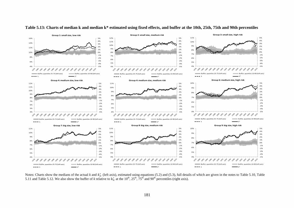
181
Table 5.13: Charts of median k and median k* estimated using fixed effects, and buffer at the 10th, 25th, 75th and 90th percentiles
Notes: Charts show the medians of the actual k and 𝑘𝑖𝑡∗ (left axis), estimated using equations (5.2) and (5.3), full details of which are given in the notes to Table 5.10, Table
5.11 and Table 5.12. We also show the buffer of k relative to kit∗ at the 10
th, 25
th, 75
th and 90
th percentiles (right axis).
-5%
-4%
-3%
-2%
-1%
0%
1%
2%
3%
4%
5%
4%
6%
8%
10%
12%
14%
16%
Group 1: small size, low risk
Buffer, quantiles 25-75 (left axis) Buffer, quantiles 10-90 (left axis)
k k*
-5%
-4%
-3%
-2%
-1%
0%
1%
2%
3%
4%
5%
4%
5%
6%
7%
8%
9%
10%
11%
12%
Group 2: small size, medium risk
Buffer, quantiles 25-75 (left axis) Buffer, quantiles 10-90 (left axis)
k k*
-5%
-4%
-3%
-2%
-1%
0%
1%
2%
3%
4%
5%
4%
5%
6%
7%
8%
9%
10%
11%
Group 3: small size, high risk
Buffer, quantiles 25-75 (left axis) Buffer, quantiles 10-90 (left axis)
k k*
-5%
-4%
-3%
-2%
-1%
0%
1%
2%
3%
4%
5%
4%
5%
6%
7%
8%
9%
10%
11%
12%
Group 4: medium size, low risk
Buffer, quantiles 25-75 (left axis) Buffer, quantiles 10-90 (left axis)
k k*
-5%
-4%
-3%
-2%
-1%
0%
1%
2%
3%
4%
5%
4%
5%
6%
7%
8%
9%
10%
11%
Group 4: medium size, medium risk
Buffer, quantiles 25-75 (left axis) Buffer, quantiles 10-90 (left axis)
k k*
-5%
-4%
-3%
-2%
-1%
0%
1%
2%
3%
4%
5%
4%
5%
6%
7%
8%
9%
10%
Group 6: medium size, high risk
Buffer, quantiles 25-75 (left axis) Buffer, quantiles 10-90 (left axis)
k k*
-5%
-4%
-3%
-2%
-1%
0%
1%
2%
3%
4%
5%
4%
5%
6%
7%
8%
9%
10%
11%
Group 7: big size, low risk
Buffer, quantiles 25-75 (left axis) Buffer, quantiles 10-90 (left axis)
k k*
-5%
-4%
-3%
-2%
-1%
0%
1%
2%
3%
4%
5%
4%
5%
6%
7%
8%
9%
10%
11%
Group 8: big size, medium risk
Buffer, quantiles 25-75 (left axis) Buffer, quantiles 10-90 (left axis)
k k*
-5%
-4%
-3%
-2%
-1%
0%
1%
2%
3%
4%
5%
4%
5%
6%
7%
8%
9%
10%
Group 9: big size, high risk
Buffer, quantiles 25-75 (left axis) Buffer, quantiles 10-90 (left axis)
k k*

182
Next, we examine the results of estimating the ROA regression (5.5) using the fixed effects
estimator. In this model, the target capital ratio and capital surplus and deficit variables are
calculated using the fixed effects estimates of the target capital ratio equation, rather than the
GMM estimates from section 5.4.2. The estimates are shown in Table 5.14, Table 5.15 and
Table 5.16 below. We compare the results to the GMM ones for three periods: the S&L
crisis period of the late 1980s, the mid-1990s and early 2000s, and the recent crisis period of
the late 2000s. Overall, we conclude that these results are consistent with the GMM results,
increasing the robustness of the economic inferences we make from the results.
First, during the late 1980s we found above that high risk banks with a capital deficit
exhibited a positive relationship between ROA and lagged k. The fixed effect findings are
consistent with this result, across small, medium and big banks. In the 1990s and early 2000s,
high risk banks with capital deficits do not exhibit a positive relationship between ROA and
lagged k, casting doubt on the idea that market discipline drove the increase in capital ratios
during this period. This finding is consistent across the GMM and fixed effect estimates.
During the crisis period, amongst banks with a capital deficit only small banks exhibited a
positive relationship between ROA and lagged k, consistent with the GMM results. Finally,
across most groups in most time periods, for banks with a capital surplus the relationship
between ROA and lagged k is negative and significant, as in the GMM results. |
The long-run coefficients on the other explanatory variables are mostly consistent with those
estimated using GMM in section 5.4.2. SIZE is positively and significantly associated with
ROA; SDROE, C&I and RW (ex ante risk measures) are positive while CHARGE and NPL
(ex post risk measures) are negative. Unlike the GMM estimates, the measures of market
power (BANKSHARE, HERF, URBAN, GROWTH) are of mixed sign and significance.
Finally, the overall R2 of the models are very high and above 0.9 in most cases, showing that
the models are a relatively good fit.
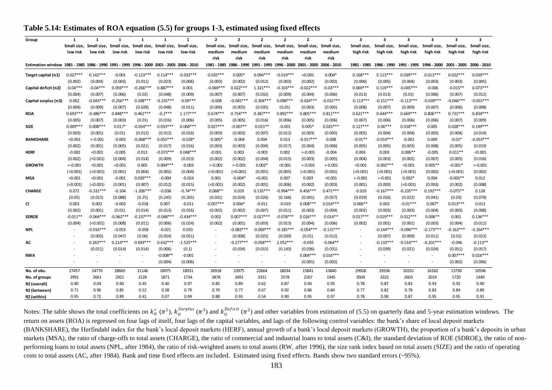
183
Table 5.14: Estimates of ROA equation (5.5) for groups 1-3, estimated using fixed effects
Notes: The table shows the total coefficients on 𝑘𝑖𝑡∗ (𝜋1), 𝑘𝑖𝑡
𝑆𝑢𝑟𝑝𝑙𝑢𝑠(𝜋3) and 𝑘𝑖𝑡
𝐷𝑒𝑓𝑖𝑐𝑖𝑡(𝜋2) and other variables from estimation of (5.5) on quarterly data and 5-year estimation windows. The
return on assets (ROA) is regressed on four lags of itself, four lags of the capital variables, and lags of the following control variables: the bank‘s share of local deposit markets
(BANKSHARE), the Herfindahl index for the bank‘s local deposit markets (HERF), annual growth of a bank‘s local deposit markets (GROWTH), the proportion of a bank‘s deposits in urban
markets (MSA), the ratio of charge-offs to total assets (CHARGE), the ratio of commercial and industrial loans to total assets (C&I), the standard deviation of ROE (SDROE), the ratio of non-
performing loans to total assets (NPL, after 1984), the ratio of risk-weighted assets to total assets (RW, after 1996), the size rank index based on total assets (SIZE) and the ratio of operating
costs to total assets (AC, after 1984). Bank and time fixed effects are included. Estimated using fixed effects. Bands show two standard errors (~95%).
Group 1 1 1 1 1 1 2 2 2 2 2 2 3 3 3 3 3 3
Small size,
low risk
Small size,
low risk
Small size,
low risk
Small size,
low risk
Small size,
low risk
Small size,
low risk
Small size,
medium
risk
Small size,
medium
risk
Small size,
medium
risk
Small size,
medium
risk
Small size,
medium
risk
Small size,
medium
risk
Small size,
high risk
Small size,
high risk
Small size,
high risk
Small size,
high risk
Small size,
high risk
Small size,
high risk
Estimation window 1981 - 1985 1986 - 1990 1991 - 1995 1996 - 2000 2001 - 2005 2006 - 2010 1981 - 1985 1986 - 1990 1991 - 1995 1996 - 2000 2001 - 2005 2006 - 2010 1981 - 1985 1986 - 1990 1991 - 1995 1996 - 2000 2001 - 2005 2006 - 2010
Target capital (π1) 0.027*** 0.142*** -0.001 -0.123*** 0.114*** -0.032*** 0.035*** 0.005* 0.094*** -0.019*** <0.001 0.004* 0.168*** 0.113*** 0.039*** 0.013*** 0.022*** 0.039***
(0.002) (0.004) (0.003) (0.011) (0.023) (0.006) (0.003) (0.002) (0.012) (0.003) (0.002) (0.002) (0.006) (0.005) (0.004) (0.003) (0.003) (0.005)
Capital deficit (π2) -0.04*** -0.04*** 0.059*** -0.266*** 0.887*** 0.001 -0.069*** 0.022*** 1.321*** -0.103*** -0.022*** -0.03*** 0.069*** 0.119*** -0.045*** -0.006 -0.015** 0.073***
(0.004) (0.007) (0.006) (0.02) (0.048) (0.009) (0.007) (0.007) (0.032) (0.009) (0.004) (0.006) (0.013) (0.013) (0.01) (0.006) (0.007) (0.012)
Capital surplus (π3) 0.002 -0.043*** -0.256*** 0.208*** -0.235*** -0.09*** -0.008 -0.045*** -0.304*** 0.098*** -0.024*** -0.031*** -0.113*** -0.151*** -0.113*** -0.039*** -0.046*** -0.055***
(0.004) (0.009) (0.007) (0.028) (0.048) (0.011) (0.006) (0.005) (0.035) (0.01) (0.003) (0.005) (0.008) (0.007) (0.009) (0.007) (0.006) (0.008)
ROA 0.693*** -0.486*** 0.848*** 0.461*** -0.2*** 1.177*** 0.674*** 0.754*** 0.387*** 0.892*** 0.805*** 0.811*** 0.621*** 0.644*** 0.669*** 0.806*** 0.731*** 0.834***
(0.005) (0.007) (0.003) (0.01) (0.016) (0.006) (0.005) (0.005) (0.016) (0.006) (0.005) (0.006) (0.007) (0.006) (0.006) (0.006) (0.007) (0.009)
SIZE 0.009*** 0.008*** 0.017* -0.054*** 0.033*** 0.068*** 0.027*** -0.007** 0.015** -0.001 0.005* 0.025*** 0.127*** 0.06*** 0.018*** 0.005 0.028*** 0.149***
(0.003) (0.001) (0.01) (0.012) (0.012) (0.016) (0.003) (0.003) (0.007) (0.012) (0.003) (0.005) (0.005) (0.004) (0.004) (0.005) (0.004) (0.014)
BANKSHARE <0.001 >-0.001 -0.003 -0.068*** 0.055*** -0.028* -0.005* -0.004 0.004 0.013 -0.017*** 0.008 -0.01** -0.014*** -0.002 0.009 -0.01* -0.053***
(0.002) (0.001) (0.005) (0.021) (0.017) (0.016) (0.003) (0.003) (0.004) (0.017) (0.004) (0.006) (0.005) (0.005) (0.003) (0.008) (0.005) (0.019)
HERF -0.002 <0.001 -0.005 0.013 -0.073*** 0.048*** -0.001 0.003 -0.003 0.002 >-0.001 -0.004 0.004 0.003 0.006** -0.005 0.011** <0.001
(0.002) (<0.001) (0.004) (0.014) (0.009) (0.013) (0.002) (0.002) (0.004) (0.015) (0.003) (0.005) (0.004) (0.003) (0.002) (0.007) (0.005) (0.016)
GROWTH >-0.001 <0.001 <0.001 0.005 0.004*** -0.003 >-0.001 >-0.001 0.002* <0.001 >-0.001 >-0.001 <0.001 -0.002*** <0.001 0.005** -0.001* >-0.001
(<0.001) (<0.001) (0.001) (0.004) (0.002) (0.004) (<0.001) (<0.001) (0.001) (0.005) (<0.001) (0.001) (<0.001) (<0.001) (<0.001) (0.002) (<0.001) (0.002)
MSA <0.001 <0.001 -0.001 0.039*** -0.004 -0.024 0.001 -0.004* <0.001 0.007 0.003 <0.001 >-0.001 >-0.001 0.002* 0.004 -0.005** 0.012
(<0.001) (<0.001) (0.001) (0.007) (0.012) (0.015) (<0.001) (0.002) (0.001) (0.006) (0.002) (0.003) (0.001) (0.003) (<0.001) (0.003) (0.002) (0.008)
CHARGE 0.072 -0.331*** -0.104 -1.206*** -0.038 -0.74*** 0.068** 0.029 0.135*** -0.994*** 0.456*** 0.471*** -0.019 -0.167*** -0.235*** 0.192*** -0.075** 0.128
(0.05) (0.015) (0.088) (0.25) (0.245) (0.265) (0.031) (0.024) (0.026) (0.166) (0.041) (0.057) (0.019) (0.016) (0.022) (0.041) (0.03) (0.079)
CI 0.003 0.002 -0.003 -0.018 0.007 -0.011 0.007*** 0.004* -0.011 -0.019 0.008*** 0.014*** 0.006** 0.003 -0.01*** 0.007* 0.013*** 0.013
(0.002) (0.001) (0.01) (0.014) (0.013) (0.016) (0.002) (0.002) (0.007) (0.011) (0.003) (0.004) (0.002) (0.003) (0.003) (0.004) (0.003) (0.008)
SDROE -0.011** -0.064*** -0.062*** -0.237*** -0.048*** -0.434*** 0.002 0.007*** 0.027*** -0.078*** 0.026*** 0.014** 0.017*** 0.019*** 0.012*** 0.006** 0.001 0.136***
(0.004) (<0.001) (0.008) (0.011) (0.006) (0.024) (0.002) (0.001) (0.003) (0.013) (0.004) (0.006) (0.002) (0.001) (0.001) (0.003) (0.004) (0.011)
NPL - -0.016*** -0.053 -0.058 -0.021 0.033 - -0.083*** -0.069*** -0.185*** -0.054*** -0.115*** - -0.144*** -0.096*** -0.173*** -0.162*** -0.264***
- (0.005) (0.047) (0.06) (0.054) (0.051) - (0.008) (0.025) (0.039) (0.01) (0.012) - (0.007) (0.009) (0.011) (0.01) (0.023)
AC - 0.263*** 0.214*** 0.693*** 0.632*** -1.525*** - -0.277*** -0.058*** 2.052*** -0.035 -0.064** - -0.133*** -0.516*** -0.201*** -0.046 -0.113**
- (0.011) (0.014) (0.014) (0.006) (0.1) - (0.034) (0.015) (0.143) (0.036) (0.031) - (0.039) (0.021) (0.024) (0.051) (0.057)
RWA - - - - -0.008** -0.001 - - - - 0.004*** 0.016*** - - - - 0.007*** 0.016***
- - - - (0.004) (0.006) - - - - (0.001) (0.002) - - - - (0.002) (0.006)
No. of obs. 27457 24776 28665 21146 18975 18931 26918 23975 22664 18034 15841 13840 29928 29336 20331 16320 13730 10596
No. of groups 2991 2661 2921 2228 1871 1734 3878 3491 3331 2578 2167 1945 3504 3325 2603 2019 1720 1449
R2 (overall) 0.90 0.04 0.90 0.45 0.40 0.97 0.85 0.89 0.62 0.87 0.94 0.95 0.78 0.87 0.83 0.93 0.92 0.90
R2 (between) 0.71 0.96 0.85 0.52 0.58 0.79 0.70 0.77 0.67 0.92 0.86 0.84 0.77 0.82 0.78 0.83 0.84 0.89
R2 (within) 0.95 0.72 0.89 0.41 0.07 0.99 0.88 0.93 0.54 0.90 0.95 0.97 0.78 0.90 0.87 0.95 0.95 0.91
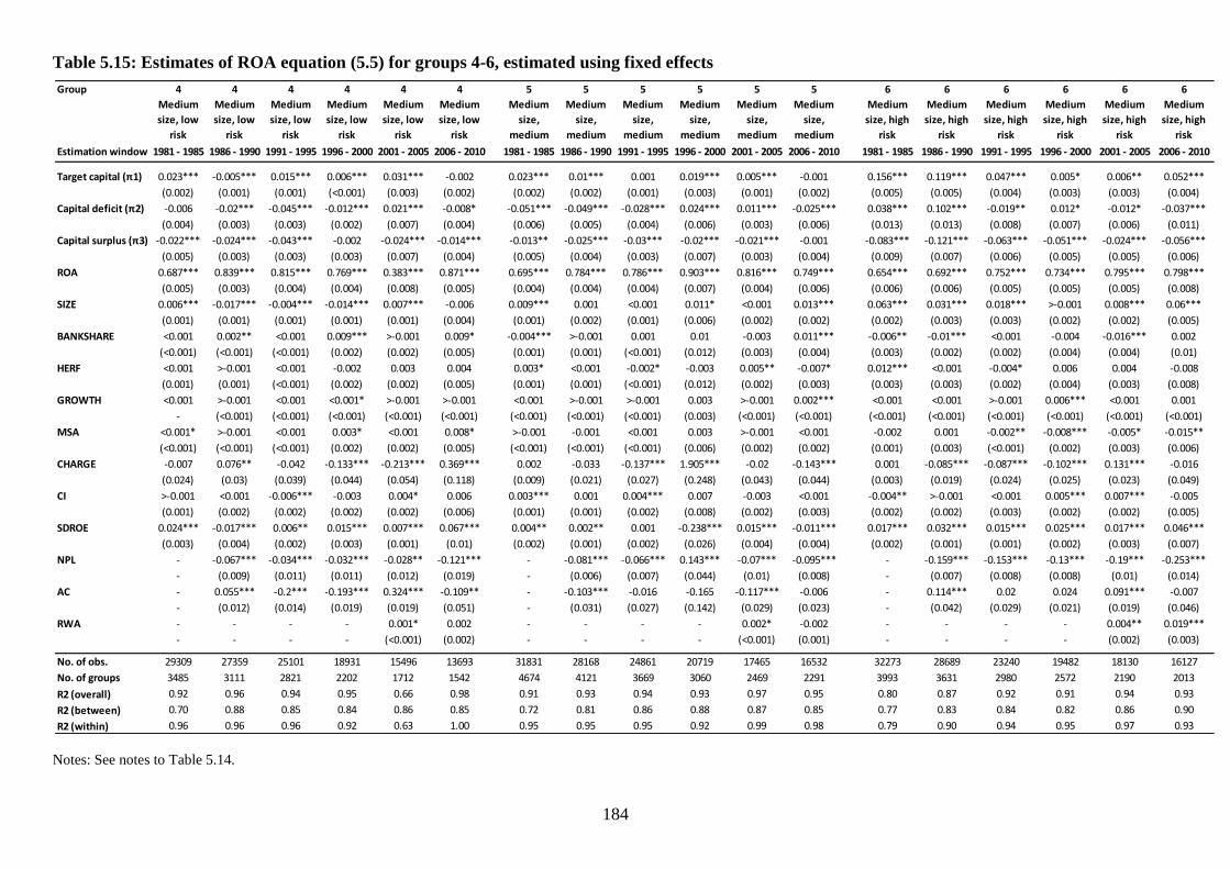
184
Table 5.15: Estimates of ROA equation (5.5) for groups 4-6, estimated using fixed effects
Notes: See notes to Table 5.14.
Group 4 4 4 4 4 4 5 5 5 5 5 5 6 6 6 6 6 6
Medium
size, low
risk
Medium
size, low
risk
Medium
size, low
risk
Medium
size, low
risk
Medium
size, low
risk
Medium
size, low
risk
Medium
size,
medium
risk
Medium
size,
medium
risk
Medium
size,
medium
risk
Medium
size,
medium
risk
Medium
size,
medium
risk
Medium
size,
medium
risk
Medium
size, high
risk
Medium
size, high
risk
Medium
size, high
risk
Medium
size, high
risk
Medium
size, high
risk
Medium
size, high
risk
Estimation window 1981 - 1985 1986 - 1990 1991 - 1995 1996 - 2000 2001 - 2005 2006 - 2010 1981 - 1985 1986 - 1990 1991 - 1995 1996 - 2000 2001 - 2005 2006 - 2010 1981 - 1985 1986 - 1990 1991 - 1995 1996 - 2000 2001 - 2005 2006 - 2010
Target capital (π1) 0.023*** -0.005*** 0.015*** 0.006*** 0.031*** -0.002 0.023*** 0.01*** 0.001 0.019*** 0.005*** -0.001 0.156*** 0.119*** 0.047*** 0.005* 0.006** 0.052***
(0.002) (0.001) (0.001) (<0.001) (0.003) (0.002) (0.002) (0.002) (0.001) (0.003) (0.001) (0.002) (0.005) (0.005) (0.004) (0.003) (0.003) (0.004)
Capital deficit (π2) -0.006 -0.02*** -0.045*** -0.012*** 0.021*** -0.008* -0.051*** -0.049*** -0.028*** 0.024*** 0.011*** -0.025*** 0.038*** 0.102*** -0.019** 0.012* -0.012* -0.037***
(0.004) (0.003) (0.003) (0.002) (0.007) (0.004) (0.006) (0.005) (0.004) (0.006) (0.003) (0.006) (0.013) (0.013) (0.008) (0.007) (0.006) (0.011)
Capital surplus (π3) -0.022*** -0.024*** -0.043*** -0.002 -0.024*** -0.014*** -0.013** -0.025*** -0.03*** -0.02*** -0.021*** -0.001 -0.083*** -0.121*** -0.063*** -0.051*** -0.024*** -0.056***
(0.005) (0.003) (0.003) (0.003) (0.007) (0.004) (0.005) (0.004) (0.003) (0.007) (0.003) (0.004) (0.009) (0.007) (0.006) (0.005) (0.005) (0.006)
ROA 0.687*** 0.839*** 0.815*** 0.769*** 0.383*** 0.871*** 0.695*** 0.784*** 0.786*** 0.903*** 0.816*** 0.749*** 0.654*** 0.692*** 0.752*** 0.734*** 0.795*** 0.798***
(0.005) (0.003) (0.004) (0.004) (0.008) (0.005) (0.004) (0.004) (0.004) (0.007) (0.004) (0.006) (0.006) (0.006) (0.005) (0.005) (0.005) (0.008)
SIZE 0.006*** -0.017*** -0.004*** -0.014*** 0.007*** -0.006 0.009*** 0.001 <0.001 0.011* <0.001 0.013*** 0.063*** 0.031*** 0.018*** >-0.001 0.008*** 0.06***
(0.001) (0.001) (0.001) (0.001) (0.001) (0.004) (0.001) (0.002) (0.001) (0.006) (0.002) (0.002) (0.002) (0.003) (0.003) (0.002) (0.002) (0.005)
BANKSHARE <0.001 0.002** <0.001 0.009*** >-0.001 0.009* -0.004*** >-0.001 0.001 0.01 -0.003 0.011*** -0.006** -0.01*** <0.001 -0.004 -0.016*** 0.002
(<0.001) (<0.001) (<0.001) (0.002) (0.002) (0.005) (0.001) (0.001) (<0.001) (0.012) (0.003) (0.004) (0.003) (0.002) (0.002) (0.004) (0.004) (0.01)
HERF <0.001 >-0.001 <0.001 -0.002 0.003 0.004 0.003* <0.001 -0.002* -0.003 0.005** -0.007* 0.012*** <0.001 -0.004* 0.006 0.004 -0.008
(0.001) (0.001) (<0.001) (0.002) (0.002) (0.005) (0.001) (0.001) (<0.001) (0.012) (0.002) (0.003) (0.003) (0.003) (0.002) (0.004) (0.003) (0.008)
GROWTH <0.001 >-0.001 <0.001 <0.001* >-0.001 >-0.001 <0.001 >-0.001 >-0.001 0.003 >-0.001 0.002*** <0.001 <0.001 >-0.001 0.006*** <0.001 0.001
- (<0.001) (<0.001) (<0.001) (<0.001) (<0.001) (<0.001) (<0.001) (<0.001) (0.003) (<0.001) (<0.001) (<0.001) (<0.001) (<0.001) (<0.001) (<0.001) (<0.001)
MSA <0.001* >-0.001 <0.001 0.003* <0.001 0.008* >-0.001 -0.001 <0.001 0.003 >-0.001 <0.001 -0.002 0.001 -0.002** -0.008*** -0.005* -0.015**
(<0.001) (<0.001) (<0.001) (0.002) (0.002) (0.005) (<0.001) (<0.001) (<0.001) (0.006) (0.002) (0.002) (0.001) (0.003) (<0.001) (0.002) (0.003) (0.006)
CHARGE -0.007 0.076** -0.042 -0.133*** -0.213*** 0.369*** 0.002 -0.033 -0.137*** 1.905*** -0.02 -0.143*** 0.001 -0.085*** -0.087*** -0.102*** 0.131*** -0.016
(0.024) (0.03) (0.039) (0.044) (0.054) (0.118) (0.009) (0.021) (0.027) (0.248) (0.043) (0.044) (0.003) (0.019) (0.024) (0.025) (0.023) (0.049)
CI >-0.001 <0.001 -0.006*** -0.003 0.004* 0.006 0.003*** 0.001 0.004*** 0.007 -0.003 <0.001 -0.004** >-0.001 <0.001 0.005*** 0.007*** -0.005
(0.001) (0.002) (0.002) (0.002) (0.002) (0.006) (0.001) (0.001) (0.002) (0.008) (0.002) (0.003) (0.002) (0.002) (0.003) (0.002) (0.002) (0.005)
SDROE 0.024*** -0.017*** 0.006** 0.015*** 0.007*** 0.067*** 0.004** 0.002** 0.001 -0.238*** 0.015*** -0.011*** 0.017*** 0.032*** 0.015*** 0.025*** 0.017*** 0.046***
(0.003) (0.004) (0.002) (0.003) (0.001) (0.01) (0.002) (0.001) (0.002) (0.026) (0.004) (0.004) (0.002) (0.001) (0.001) (0.002) (0.003) (0.007)
NPL - -0.067*** -0.034*** -0.032*** -0.028** -0.121*** - -0.081*** -0.066*** 0.143*** -0.07*** -0.095*** - -0.159*** -0.153*** -0.13*** -0.19*** -0.253***
- (0.009) (0.011) (0.011) (0.012) (0.019) - (0.006) (0.007) (0.044) (0.01) (0.008) - (0.007) (0.008) (0.008) (0.01) (0.014)
AC - 0.055*** -0.2*** -0.193*** 0.324*** -0.109** - -0.103*** -0.016 -0.165 -0.117*** -0.006 - 0.114*** 0.02 0.024 0.091*** -0.007
- (0.012) (0.014) (0.019) (0.019) (0.051) - (0.031) (0.027) (0.142) (0.029) (0.023) - (0.042) (0.029) (0.021) (0.019) (0.046)
RWA - - - - 0.001* 0.002 - - - - 0.002* -0.002 - - - - 0.004** 0.019***
- - - - (<0.001) (0.002) - - - - (<0.001) (0.001) - - - - (0.002) (0.003)
No. of obs. 29309 27359 25101 18931 15496 13693 31831 28168 24861 20719 17465 16532 32273 28689 23240 19482 18130 16127
No. of groups 3485 3111 2821 2202 1712 1542 4674 4121 3669 3060 2469 2291 3993 3631 2980 2572 2190 2013
R2 (overall) 0.92 0.96 0.94 0.95 0.66 0.98 0.91 0.93 0.94 0.93 0.97 0.95 0.80 0.87 0.92 0.91 0.94 0.93
R2 (between) 0.70 0.88 0.85 0.84 0.86 0.85 0.72 0.81 0.86 0.88 0.87 0.85 0.77 0.83 0.84 0.82 0.86 0.90
R2 (within) 0.96 0.96 0.96 0.92 0.63 1.00 0.95 0.95 0.95 0.92 0.99 0.98 0.79 0.90 0.94 0.95 0.97 0.93
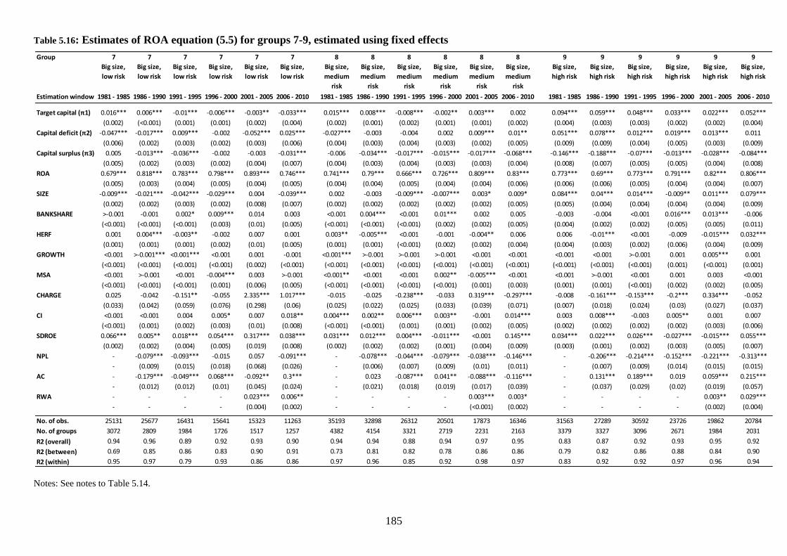
185
Table 5.16: Estimates of ROA equation (5.5) for groups 7-9, estimated using fixed effects
Notes: See notes to Table 5.14.
Group 7 7 7 7 7 7 8 8 8 8 8 8 9 9 9 9 9 9
Big size,
low risk
Big size,
low risk
Big size,
low risk
Big size,
low risk
Big size,
low risk
Big size,
low risk
Big size,
medium
risk
Big size,
medium
risk
Big size,
medium
risk
Big size,
medium
risk
Big size,
medium
risk
Big size,
medium
risk
Big size,
high risk
Big size,
high risk
Big size,
high risk
Big size,
high risk
Big size,
high risk
Big size,
high risk
Estimation window 1981 - 1985 1986 - 1990 1991 - 1995 1996 - 2000 2001 - 2005 2006 - 2010 1981 - 1985 1986 - 1990 1991 - 1995 1996 - 2000 2001 - 2005 2006 - 2010 1981 - 1985 1986 - 1990 1991 - 1995 1996 - 2000 2001 - 2005 2006 - 2010
Target capital (π1) 0.016*** 0.006*** -0.01*** -0.006*** -0.003** -0.033*** 0.015*** 0.008*** -0.008*** -0.002** 0.003*** 0.002 0.094*** 0.059*** 0.048*** 0.033*** 0.022*** 0.052***
(0.002) (<0.001) (0.001) (0.001) (0.002) (0.004) (0.002) (0.001) (0.002) (0.001) (0.001) (0.002) (0.004) (0.003) (0.003) (0.002) (0.002) (0.004)
Capital deficit (π2) -0.047*** -0.017*** 0.009*** -0.002 -0.052*** 0.025*** -0.027*** -0.003 -0.004 0.002 0.009*** 0.01** 0.051*** 0.078*** 0.012*** 0.019*** 0.013*** 0.011
(0.006) (0.002) (0.003) (0.002) (0.003) (0.006) (0.004) (0.003) (0.004) (0.003) (0.002) (0.005) (0.009) (0.009) (0.004) (0.005) (0.003) (0.009)
Capital surplus (π3) 0.005 -0.013*** -0.036*** -0.002 -0.003 -0.031*** -0.006 -0.034*** -0.017*** -0.015*** -0.017*** -0.068*** -0.146*** -0.188*** -0.07*** -0.013*** -0.028*** -0.084***
(0.005) (0.002) (0.003) (0.002) (0.004) (0.007) (0.004) (0.003) (0.004) (0.003) (0.003) (0.004) (0.008) (0.007) (0.005) (0.005) (0.004) (0.008)
ROA 0.679*** 0.818*** 0.783*** 0.798*** 0.893*** 0.746*** 0.741*** 0.79*** 0.666*** 0.726*** 0.809*** 0.83*** 0.773*** 0.69*** 0.773*** 0.791*** 0.82*** 0.806***
(0.005) (0.003) (0.004) (0.005) (0.004) (0.005) (0.004) (0.004) (0.005) (0.004) (0.004) (0.006) (0.006) (0.006) (0.005) (0.004) (0.004) (0.007)
SIZE -0.009*** -0.021*** -0.042*** -0.029*** 0.004 -0.039*** 0.002 -0.003 -0.009*** -0.007*** 0.003* 0.009* 0.084*** 0.04*** 0.014*** -0.009** 0.011*** 0.079***
(0.002) (0.002) (0.003) (0.002) (0.008) (0.007) (0.002) (0.002) (0.002) (0.002) (0.002) (0.005) (0.005) (0.004) (0.004) (0.004) (0.004) (0.009)
BANKSHARE >-0.001 -0.001 0.002* 0.009*** 0.014 0.003 <0.001 0.004*** <0.001 0.01*** 0.002 0.005 -0.003 -0.004 <0.001 0.016*** 0.013*** -0.006
(<0.001) (<0.001) (<0.001) (0.003) (0.01) (0.005) (<0.001) (<0.001) (<0.001) (0.002) (0.002) (0.005) (0.004) (0.002) (0.002) (0.005) (0.005) (0.011)
HERF 0.001 0.004*** -0.003** -0.002 0.007 0.001 0.003** -0.005*** <0.001 -0.001 -0.004** 0.006 0.006 -0.01*** <0.001 -0.009 -0.015*** 0.032***
(0.001) (0.001) (0.001) (0.002) (0.01) (0.005) (0.001) (0.001) (<0.001) (0.002) (0.002) (0.004) (0.004) (0.003) (0.002) (0.006) (0.004) (0.009)
GROWTH <0.001 >-0.001*** <0.001*** <0.001 0.001 -0.001 <0.001*** >-0.001 >-0.001 >-0.001 <0.001 <0.001 <0.001 <0.001 >-0.001 0.001 0.005*** 0.001
(<0.001) (<0.001) (<0.001) (<0.001) (0.002) (<0.001) (<0.001) (<0.001) (<0.001) (<0.001) (<0.001) (<0.001) (<0.001) (<0.001) (<0.001) (0.001) (<0.001) (0.001)
MSA <0.001 >-0.001 <0.001 -0.004*** 0.003 >-0.001 <0.001** <0.001 <0.001 0.002** -0.005*** <0.001 <0.001 >-0.001 <0.001 0.001 0.003 <0.001
(<0.001) (<0.001) (<0.001) (0.001) (0.006) (0.005) (<0.001) (<0.001) (<0.001) (<0.001) (0.001) (0.003) (0.001) (0.001) (<0.001) (0.002) (0.002) (0.005)
CHARGE 0.025 -0.042 -0.151** -0.055 2.335*** 1.017*** -0.015 -0.025 -0.238*** -0.033 0.319*** -0.297*** -0.008 -0.161*** -0.153*** -0.2*** 0.334*** -0.052
(0.033) (0.042) (0.059) (0.076) (0.298) (0.06) (0.025) (0.022) (0.025) (0.033) (0.039) (0.071) (0.007) (0.018) (0.024) (0.03) (0.027) (0.037)
CI <0.001 <0.001 0.004 0.005* 0.007 0.018** 0.004*** 0.002** 0.006*** 0.003** -0.001 0.014*** 0.003 0.008*** -0.003 0.005** 0.001 0.007
(<0.001) (0.001) (0.002) (0.003) (0.01) (0.008) (<0.001) (<0.001) (0.001) (0.001) (0.002) (0.005) (0.002) (0.002) (0.002) (0.002) (0.003) (0.006)
SDROE 0.066*** 0.005** 0.018*** 0.054*** 0.317*** 0.038*** 0.031*** 0.012*** 0.004*** -0.011*** <0.001 0.145*** 0.034*** 0.022*** 0.026*** -0.027*** -0.015*** 0.055***
(0.002) (0.002) (0.004) (0.005) (0.019) (0.008) (0.002) (0.002) (0.002) (0.001) (0.004) (0.009) (0.003) (0.001) (0.002) (0.003) (0.005) (0.007)
NPL - -0.079*** -0.093*** -0.015 0.057 -0.091*** - -0.078*** -0.044*** -0.079*** -0.038*** -0.146*** - -0.206*** -0.214*** -0.152*** -0.221*** -0.313***
- (0.009) (0.015) (0.018) (0.068) (0.026) - (0.006) (0.007) (0.009) (0.01) (0.011) - (0.007) (0.009) (0.014) (0.015) (0.015)
AC - -0.179*** -0.049*** 0.068*** -0.092** 0.3*** - 0.023 -0.087*** 0.041** -0.088*** -0.116*** - 0.131*** 0.189*** 0.019 0.059*** 0.215***
- (0.012) (0.012) (0.01) (0.045) (0.024) - (0.021) (0.018) (0.019) (0.017) (0.039) - (0.037) (0.029) (0.02) (0.019) (0.057)
RWA - - - - 0.023*** 0.006** - - - - 0.003*** 0.003* - - - - 0.003** 0.029***
- - - - (0.004) (0.002) - - - - (<0.001) (0.002) - - - - (0.002) (0.004)
No. of obs. 25131 25677 16431 15641 15323 11263 35193 32898 26312 20501 17873 16346 31563 27289 30592 23726 19862 20784
No. of groups 3072 2809 1984 1726 1517 1257 4382 4154 3321 2719 2231 2163 3379 3327 3096 2671 1984 2031
R2 (overall) 0.94 0.96 0.89 0.92 0.93 0.90 0.94 0.94 0.88 0.94 0.97 0.95 0.83 0.87 0.92 0.93 0.95 0.92
R2 (between) 0.69 0.85 0.86 0.83 0.90 0.91 0.73 0.81 0.82 0.78 0.86 0.86 0.79 0.82 0.86 0.88 0.84 0.90
R2 (within) 0.95 0.97 0.79 0.93 0.86 0.86 0.97 0.96 0.85 0.92 0.98 0.97 0.83 0.92 0.92 0.97 0.96 0.94
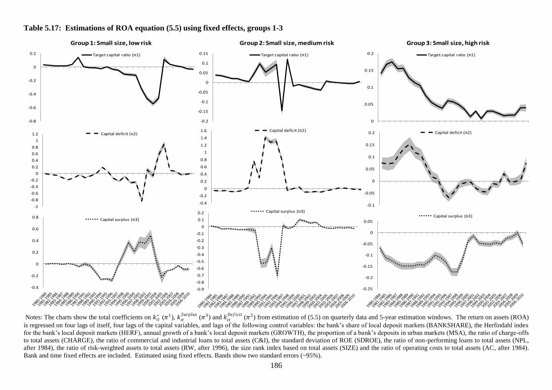
186
Table 5.17: Estimations of ROA equation (5.5) using fixed effects, groups 1-3
Notes: The charts show the total coefficients on 𝑘𝑖𝑡∗ (𝜋1), 𝑘𝑖𝑡
𝑆𝑢𝑟𝑝𝑙𝑢𝑠(𝜋3) and 𝑘𝑖𝑡
𝐷𝑒𝑓𝑖𝑐𝑖𝑡(𝜋2) from estimation of (5.5) on quarterly data and 5-year estimation windows. The return on assets (ROA)
is regressed on four lags of itself, four lags of the capital variables, and lags of the following control variables: the bank‘s share of local deposit markets (BANKSHARE), the Herfindahl index
for the bank‘s local deposit markets (HERF), annual growth of a bank‘s local deposit markets (GROWTH), the proportion of a bank‘s deposits in urban markets (MSA), the ratio of charge-offs
to total assets (CHARGE), the ratio of commercial and industrial loans to total assets (C&I), the standard deviation of ROE (SDROE), the ratio of non-performing loans to total assets (NPL,
after 1984), the ratio of risk-weighted assets to total assets (RW, after 1996), the size rank index based on total assets (SIZE) and the ratio of operating costs to total assets (AC, after 1984).
Bank and time fixed effects are included. Estimated using fixed effects. Bands show two standard errors (~95%).
-0.8
-0.6
-0.4
-0.2
0
0.2
Group 1: Small size, low risk
Target capital ratio (π1)
-1
-0.8
-0.6
-0.4
-0.2
0
0.2
0.4
0.6
0.8
1
1.2 Capital deficit (π2)
-0.2
-0.15
-0.1
-0.05
0
0.05
0.1
0.15
Group 2: Small size, medium risk
Target capital ratio (π1)
-0.4
-0.2
0
0.2
0.4
0.6
0.8
1
1.2
1.4
1.6 Capital deficit (π2)
0
0.05
0.1
0.15
0.2
Group 3: Small size, high risk
Target capital ratio (π1)
-0.1
-0.05
0
0.05
0.1
0.15
0.2 Capital deficit (π2)
-0.4
-0.2
0
0.2
0.4
0.6
0.8Capital surplus (π3)
-0.9
-0.8
-0.7
-0.6
-0.5
-0.4
-0.3
-0.2
-0.1
0
0.1
0.2 Capital surplus (π3)
-0.25
-0.2
-0.15
-0.1
-0.05
0
0.05Capital surplus (π3)

187
Table 5.18: Estimations of ROA equation (5.4) using fixed effects, groups 4-6
Notes: See notes to Table 5.17.
-0.02
-0.01
0
0.01
0.02
0.03
0.04
0.05
Group 4: Medium size, low risk
Target capital ratio (π1)
-0.1
-0.05
0
0.05
0.1 Capital deficit (π2)
-0.1
-0.05
0
0.05 Capital surplus (π3)
-0.02
-0.01
0
0.01
0.02
0.03
0.04
0.05
Group 5: Medium size, medium risk
Target capital ratio (π1)
-0.15
-0.1
-0.05
0
0.05 Capital deficit (π2)
-0.1
-0.05
0
0.05
0.1 Capital surplus (π3)
-0.05
0
0.05
0.1
0.15
0.2
Group 6: Medium size, high risk
Target capital ratio (π1)
-0.1
-0.05
0
0.05
0.1
0.15 Capital deficit (π2)
-0.2
-0.15
-0.1
-0.05
0Capital surplus (π3)
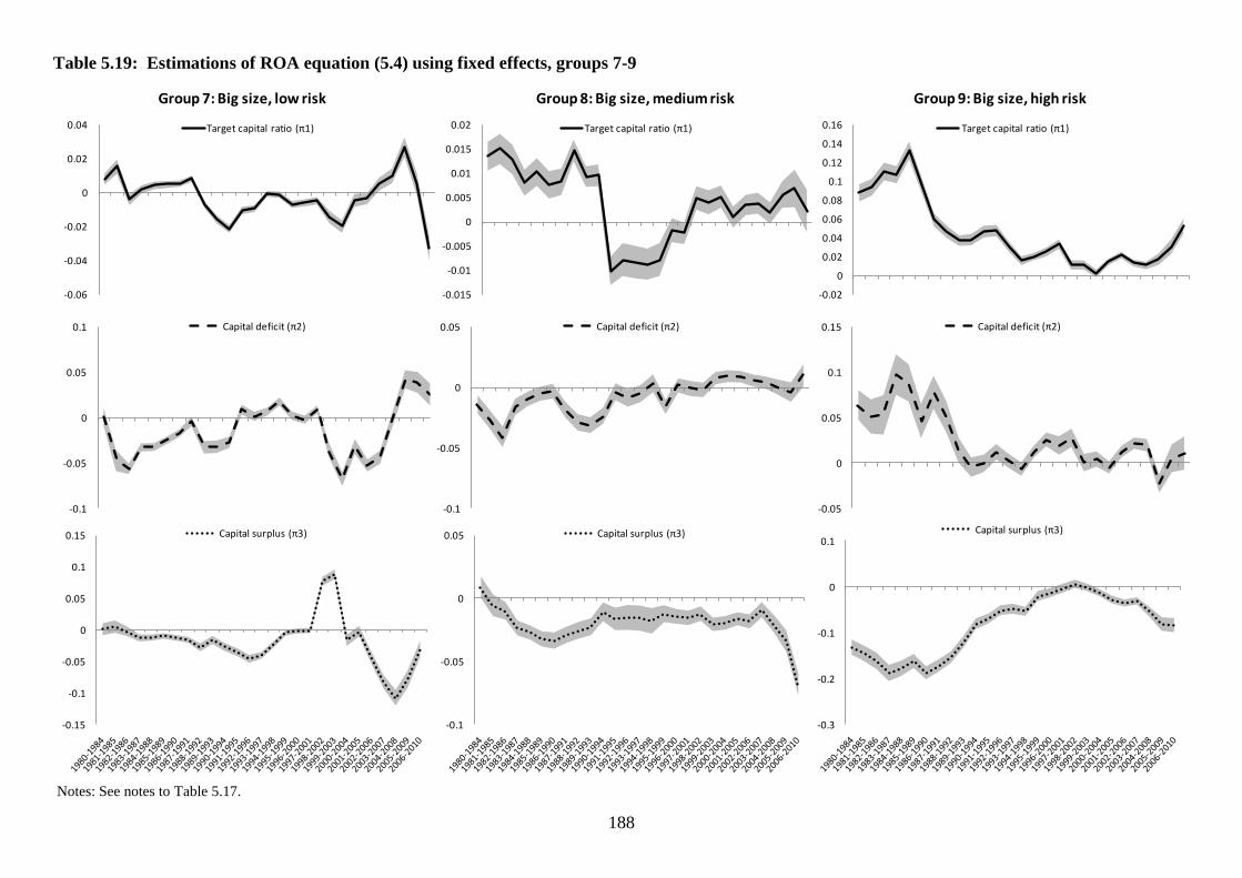
188
Table 5.19: Estimations of ROA equation (5.4) using fixed effects, groups 7-9
Notes: See notes to Table 5.17.
-0.06
-0.04
-0.02
0
0.02
0.04
Group 7: Big size, low risk
Target capital ratio (π1)
-0.1
-0.05
0
0.05
0.1 Capital deficit (π2)
-0.15
-0.1
-0.05
0
0.05
0.1
0.15 Capital surplus (π3)
-0.015
-0.01
-0.005
0
0.005
0.01
0.015
0.02
Group 8: Big size, medium risk
Target capital ratio (π1)
-0.1
-0.05
0
0.05 Capital deficit (π2)
-0.1
-0.05
0
0.05 Capital surplus (π3)
-0.02
0
0.02
0.04
0.06
0.08
0.1
0.12
0.14
0.16
Group 9: Big size, high risk
Target capital ratio (π1)
-0.05
0
0.05
0.1
0.15 Capital deficit (π2)
-0.3
-0.2
-0.1
0
0.1Capital surplus (π3)
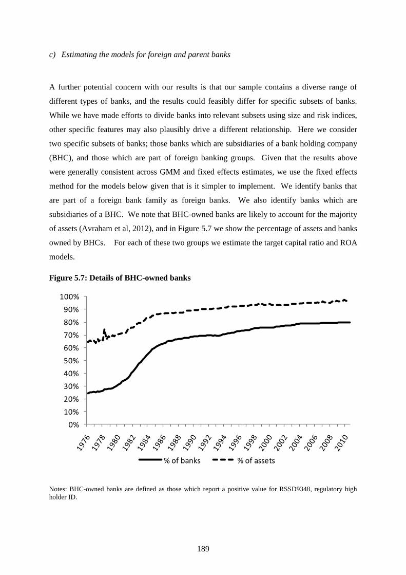
189
c) Estimating the models for foreign and parent banks
A further potential concern with our results is that our sample contains a diverse range of
different types of banks, and the results could feasibly differ for specific subsets of banks.
While we have made efforts to divide banks into relevant subsets using size and risk indices,
other specific features may also plausibly drive a different relationship. Here we consider
two specific subsets of banks; those banks which are subsidiaries of a bank holding company
(BHC), and those which are part of foreign banking groups. Given that the results above
were generally consistent across GMM and fixed effects estimates, we use the fixed effects
method for the models below given that is it simpler to implement. We identify banks that
are part of a foreign bank family as foreign banks. We also identify banks which are
subsidiaries of a BHC. We note that BHC-owned banks are likely to account for the majority
of assets (Avraham et al, 2012), and in Figure 5.7 we show the percentage of assets and banks
owned by BHCs. For each of these two groups we estimate the target capital ratio and ROA
models.
Figure 5.7: Details of BHC-owned banks
Notes: BHC-owned banks are defined as those which report a positive value for RSSD9348, regulatory high
holder ID.
0%
10%
20%
30%
40%
50%
60%
70%
80%
90%
100%
% of banks % of assets

190
For these two groups of banks, we show the target capital ratio models in Table 5.20, the
target capital ratios and capital buffers in Figure 5.8, the ROA models in Error! Reference
source not found., and the charts of the estimated effect of the capital variables on ROA in
Figure 5.9. Considering foreign banks first, the sample size is much smaller than for the
groups above (around 70-130 banks) and the models for these banks do not perform as well
as the models above. While we are able to estimate a fairly close fit for the target capital
ratio as shown in Figure 5.8, the R2 for these regressions is lower than for the regressions
above at around 0.4-0.6. Furthermore, the ROA models are inconclusive about whether
capital surpluses and deficits are important determinants of ROA, since the estimates in
Figure 5.9 are volatile and do not follow any pattern. This may indicate that the sample is too
small or that particular idiosyncratic factors drive the results for foreign banks.
Turning to the results for BHC-owned banks, we note that for much of the sample period
these banks account for the vast majority of our dataset in terms of number of banks and total
assets. Hence, this exercise is close to examining the whole sample rather than dividing them
into SIZE-RISK groups as we have done above. This may well result in a loss of valuable
information on the determinants of each bank‘s capital ratio and ROA, since it forces
homogenous specifications for the target capital ratio and ROA equations onto banks with
very different business models. Nonetheless, the results are similar to those above in some
respects. In the late 1980s, we observe a positive association between lagged capital deficits
and ROA, consistent with the results above. However, in the mid-1990s and 2000s, and in
the recent crisis period, the results are not consistent with the models above, suggesting that
our more granular division of banks by SIZE and RISK performs better in uncovering the
economic relationships of interest.
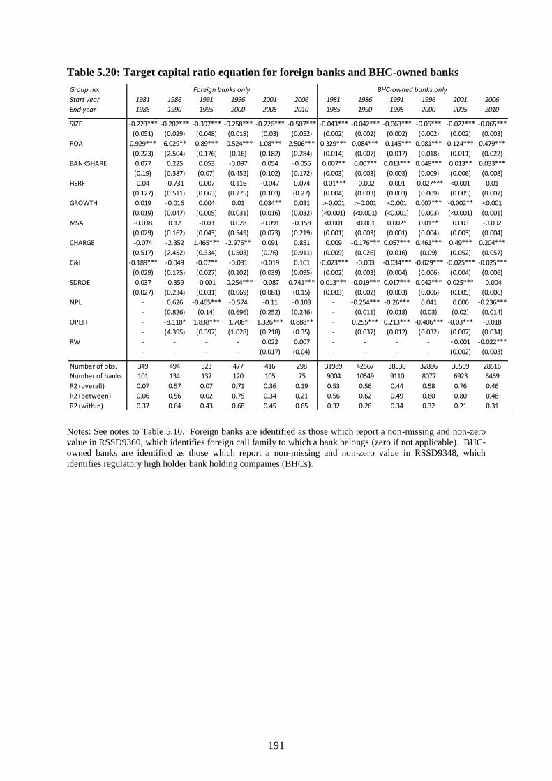
191
Table 5.20: Target capital ratio equation for foreign banks and BHC-owned banks
Notes: See notes to Table 5.10. Foreign banks are identified as those which report a non-missing and non-zero
value in RSSD9360, which identifies foreign call family to which a bank belongs (zero if not applicable). BHC-
owned banks are identified as those which report a non-missing and non-zero value in RSSD9348, which
identifies regulatory high holder bank holding companies (BHCs).
Group no.
Start year 1981 1986 1991 1996 2001 2006 1981 1986 1991 1996 2001 2006
End year 1985 1990 1995 2000 2005 2010 1985 1990 1995 2000 2005 2010
SIZE -0.223*** -0.202*** -0.397*** -0.258*** -0.226*** -0.507*** -0.043*** -0.042*** -0.063*** -0.06*** -0.022*** -0.065***
(0.051) (0.029) (0.048) (0.018) (0.03) (0.052) (0.002) (0.002) (0.002) (0.002) (0.002) (0.003)
ROA 0.929*** 6.029** 0.89*** -0.524*** 1.08*** 2.506*** 0.329*** 0.084*** -0.145*** 0.081*** 0.124*** 0.479***
(0.223) (2.504) (0.176) (0.16) (0.182) (0.284) (0.014) (0.007) (0.017) (0.018) (0.011) (0.022)
BANKSHARE 0.077 0.225 0.053 -0.097 0.054 -0.055 0.007** 0.007** 0.013*** 0.049*** 0.013** 0.033***
(0.19) (0.387) (0.07) (0.452) (0.102) (0.172) (0.003) (0.003) (0.003) (0.009) (0.006) (0.008)
HERF 0.04 -0.731 0.007 0.116 -0.047 0.074 -0.01*** -0.002 0.001 -0.027*** <0.001 0.01
(0.127) (0.511) (0.063) (0.275) (0.103) (0.27) (0.004) (0.003) (0.003) (0.009) (0.005) (0.007)
GROWTH 0.019 -0.016 0.004 0.01 0.034** 0.031 >-0.001 >-0.001 <0.001 0.007*** -0.002** <0.001
(0.019) (0.047) (0.005) (0.031) (0.016) (0.032) (<0.001) (<0.001) (<0.001) (0.003) (<0.001) (0.001)
MSA -0.038 0.12 -0.03 0.028 -0.091 -0.158 <0.001 <0.001 0.002* 0.01** 0.003 -0.002
(0.029) (0.162) (0.043) (0.549) (0.073) (0.219) (0.001) (0.003) (0.001) (0.004) (0.003) (0.004)
CHARGE -0.074 -2.352 1.465*** -2.975** 0.091 0.851 0.009 -0.176*** 0.057*** 0.461*** 0.49*** 0.204***
(0.517) (2.452) (0.334) (1.503) (0.76) (0.911) (0.009) (0.026) (0.016) (0.09) (0.052) (0.057)
C&I -0.189*** -0.049 -0.07** -0.031 -0.019 0.101 -0.023*** -0.003 -0.034*** -0.029*** -0.025*** -0.025***
(0.029) (0.175) (0.027) (0.102) (0.039) (0.095) (0.002) (0.003) (0.004) (0.006) (0.004) (0.006)
SDROE 0.037 -0.359 -0.001 -0.254*** -0.087 0.741*** 0.013*** -0.019*** 0.017*** 0.042*** 0.025*** -0.004
(0.027) (0.234) (0.031) (0.069) (0.081) (0.15) (0.003) (0.002) (0.003) (0.006) (0.005) (0.006)
NPL - 0.626 -0.465*** -0.574 -0.11 -0.103 - -0.254*** -0.26*** 0.041 0.006 -0.236***
- (0.826) (0.14) (0.696) (0.252) (0.246) - (0.011) (0.018) (0.03) (0.02) (0.014)
OPEFF - -8.118* 1.838*** 1.708* 1.326*** 0.888** - 0.255*** 0.213*** -0.406*** -0.03*** -0.018
- (4.395) (0.397) (1.028) (0.218) (0.35) - (0.037) (0.012) (0.032) (0.007) (0.034)
RW - - - - 0.022 0.007 - - - - <0.001 -0.022***
- - - - (0.017) (0.04) - - - - (0.002) (0.003)
Number of obs. 349 494 523 477 416 298 31989 42567 38530 32896 30569 28516
Number of banks 101 134 137 120 105 75 9004 10549 9110 8077 6923 6469
R2 (overall) 0.07 0.57 0.07 0.71 0.36 0.19 0.53 0.56 0.44 0.58 0.76 0.46
R2 (between) 0.06 0.56 0.02 0.75 0.34 0.21 0.56 0.62 0.49 0.60 0.80 0.48
R2 (within) 0.37 0.64 0.43 0.68 0.45 0.65 0.32 0.26 0.34 0.32 0.21 0.31
Foreign banks only BHC-owned banks only

192
Figure 5.8: Charts of median k and median k* estimated for foreign and BHC-owned
banks only using fixed effects, and buffer at the 10th, 25th, 75th and 90th percentiles
Notes: See notes to Figure 5.5 and Table 5.20.
-0.15
-0.1
-0.05
0
0.05
0.1
0.15
Foreign banks only
Target capital ratio (π1)
-0.2
-0.15
-0.1
-0.05
0
0.05
0.1
0.15 Capital deficit (π2)
-0.25
-0.2
-0.15
-0.1
-0.05
0
0.05
0.1
0.15
0.2 Capital surplus (π3)
-0.3
-0.2
-0.1
0
0.1
0.2
BHC-owned banks only
Target capital ratio (π1)
-0.4
-0.35
-0.3
-0.25
-0.2
-0.15
-0.1
-0.05
0
0.05
0.1
0.15 Capital deficit (π2)
-0.2
-0.15
-0.1
-0.05
0
0.05
0.1
0.15
0.2
0.25
0.3 Capital surplus (π3)
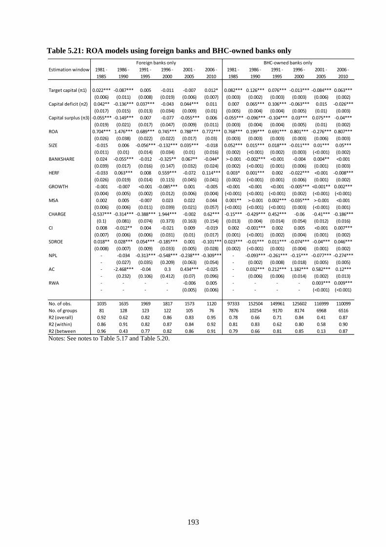
193
Table 5.21: ROA models using foreign banks and BHC-owned banks only
Notes: See notes to Table 5.17 and Table 5.20.
Estimation window 1981 -
1985
1986 -
1990
1991 -
1995
1996 -
2000
2001 -
2005
2006 -
2010
1981 -
1985
1986 -
1990
1991 -
1995
1996 -
2000
2001 -
2005
2006 -
2010
Target capital (π1) 0.022*** -0.087*** 0.005 -0.011 -0.007 0.012* 0.082*** 0.126*** 0.076*** -0.013*** -0.084*** 0.063***
(0.006) (0.011) (0.008) (0.019) (0.006) (0.007) (0.003) (0.002) (0.003) (0.003) (0.006) (0.002)
Capital deficit (π2) 0.042** -0.136*** 0.037*** -0.043 0.044*** 0.011 0.007 0.065*** 0.106*** -0.063*** 0.015 -0.026***
(0.017) (0.015) (0.013) (0.034) (0.009) (0.01) (0.005) (0.004) (0.004) (0.005) (0.01) (0.003)
Capital surplus (π3) -0.055*** -0.149*** 0.007 -0.077 -0.055*** 0.006 -0.055*** -0.096*** -0.104*** 0.03*** 0.075*** -0.04***
(0.019) (0.021) (0.017) (0.047) (0.009) (0.011) (0.003) (0.004) (0.004) (0.005) (0.01) (0.002)
ROA 0.704*** 1.476*** 0.689*** 0.745*** 0.788*** 0.772*** 0.768*** 0.199*** 0.691*** 0.801*** -0.276*** 0.807***
(0.026) (0.038) (0.022) (0.022) (0.017) (0.03) (0.003) (0.003) (0.003) (0.003) (0.006) (0.003)
SIZE -0.015 0.006 -0.056*** -0.132*** 0.035*** -0.018 0.052*** 0.015*** 0.018*** -0.011*** 0.01*** 0.05***
(0.011) (0.01) (0.014) (0.034) (0.01) (0.016) (0.002) (<0.001) (0.002) (0.003) (<0.001) (0.002)
BANKSHARE 0.024 -0.055*** -0.012 -0.325** 0.067** -0.044* >-0.001 -0.002*** <0.001 -0.004 0.004** <0.001
(0.039) (0.017) (0.016) (0.147) (0.032) (0.024) (0.002) (<0.001) (0.001) (0.006) (0.001) (0.003)
HERF -0.033 0.063*** 0.008 0.559*** -0.072 0.114*** 0.003* 0.001*** 0.002 -0.022*** <0.001 -0.008***
(0.026) (0.019) (0.014) (0.115) (0.045) (0.041) (0.002) (<0.001) (0.001) (0.006) (0.001) (0.002)
GROWTH -0.001 -0.007 <0.001 -0.085*** 0.001 -0.005 <0.001 <0.001 <0.001 -0.005*** <0.001** 0.002***
(0.004) (0.005) (0.002) (0.012) (0.006) (0.004) (<0.001) (<0.001) (<0.001) (0.002) (<0.001) (<0.001)
MSA 0.002 0.005 -0.007 0.023 0.022 0.044 0.001** >-0.001 0.002*** -0.035*** >-0.001 <0.001
(0.006) (0.006) (0.011) (0.039) (0.021) (0.057) (<0.001) (<0.001) (<0.001) (0.003) (<0.001) (0.001)
CHARGE -0.537*** -0.314*** -0.388*** 1.944*** -0.002 0.62*** -0.15*** -0.429*** 0.452*** -0.06 -0.41*** -0.186***
(0.1) (0.081) (0.074) (0.373) (0.163) (0.154) (0.013) (0.004) (0.014) (0.054) (0.012) (0.016)
CI 0.008 -0.012** 0.004 -0.021 0.009 -0.019 0.002 -0.001*** 0.002 0.005 <0.001 0.007***
(0.007) (0.006) (0.006) (0.031) (0.01) (0.017) (0.001) (<0.001) (0.002) (0.004) (0.001) (0.002)
SDROE 0.018** 0.028*** 0.054*** -0.185*** 0.001 -0.101*** 0.023*** -0.01*** 0.011*** -0.074*** -0.04*** 0.046***
(0.008) (0.007) (0.009) (0.033) (0.005) (0.028) (0.002) (<0.001) (0.001) (0.004) (0.001) (0.002)
NPL - -0.034 -0.313*** -0.548*** -0.238*** -0.309*** - -0.093*** -0.261*** -0.15*** -0.077*** -0.274***
- (0.027) (0.035) (0.209) (0.063) (0.054) - (0.002) (0.008) (0.018) (0.005) (0.005)
AC - -2.468*** -0.04 0.3 0.434*** -0.025 - 0.032*** 0.212*** 1.182*** 0.582*** 0.12***
- (0.232) (0.106) (0.412) (0.07) (0.096) - (0.006) (0.006) (0.014) (0.002) (0.013)
RWA - - - - -0.006 0.005 - - - - 0.003*** 0.009***
- - - - (0.005) (0.006) - - - - (<0.001) (<0.001)
No. of obs. 1035 1635 1969 1817 1573 1120 97333 152504 149961 125602 116999 110099
No. of groups 81 128 123 122 105 76 7876 10254 9170 8174 6968 6516
R2 (overall) 0.92 0.62 0.82 0.86 0.83 0.95 0.78 0.66 0.71 0.84 0.41 0.87
R2 (within) 0.86 0.91 0.82 0.87 0.84 0.92 0.81 0.83 0.62 0.80 0.58 0.90
R2 (between 0.96 0.43 0.77 0.82 0.86 0.91 0.79 0.66 0.81 0.85 0.13 0.87
Foreign banks only BHC-owned banks only

194
Figure 5.9: ROA models for foreign banks and BHC-owned banks
Notes: See notes to Figure 5.6 and Table 5.20. Target capital ratio is estimated for these banks only as shown in
Table 5.20.
d) Using squared capital in ROA model
Our final robustness check concerns whether our estimation of bank-specific target capital
ratios for each SIZE-RISK group is justified. An alternative and simpler way of identifying
curvature and optimality in the relationships between variables is to introduce non-linearity
by including a squared as well as a linear term in the ROA equation (5.5). Then there is no
need to estimate target capital ratio equation (5.2), and the ROA equation (5.5) becomes:
-0.15
-0.1
-0.05
0
0.05
0.1
0.15
Foreign banks only
Target capital ratio (π1)
-0.2
-0.15
-0.1
-0.05
0
0.05
0.1
0.15 Capital deficit (π2)
-0.25
-0.2
-0.15
-0.1
-0.05
0
0.05
0.1
0.15
0.2 Capital surplus (π3)
-0.3
-0.2
-0.1
0
0.1
0.2
BHC-owned banks only
Target capital ratio (π1)
-0.4
-0.35
-0.3
-0.25
-0.2
-0.15
-0.1
-0.05
0
0.05
0.1
0.15 Capital deficit (π2)
-0.2
-0.15
-0.1
-0.05
0
0.05
0.1
0.15
0.2
0.25
0.3 Capital surplus (π3)
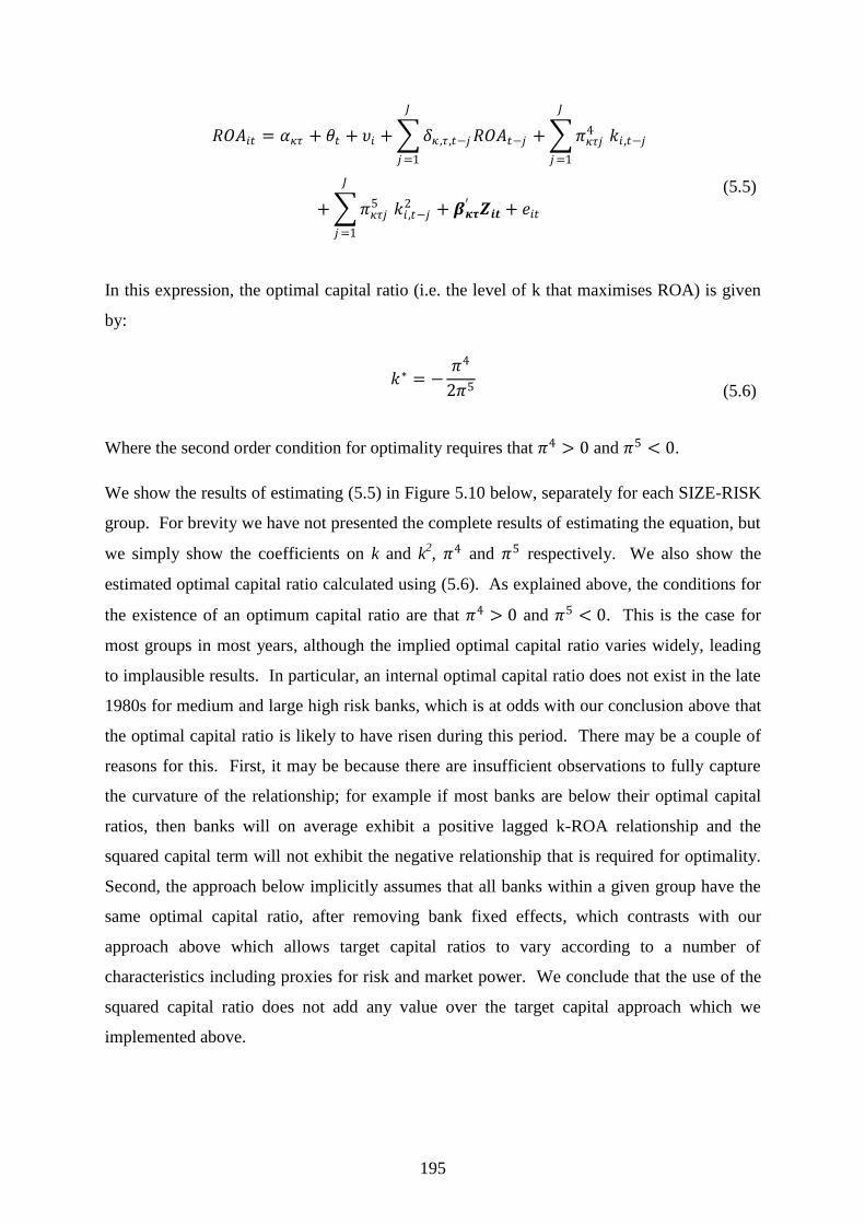
195
𝑅𝑂𝐴𝑖𝑡 = 𝛼𝜅𝜏 + 𝜃𝑡 + 𝜐𝑖 + 𝛿𝜅 ,𝜏 ,𝑡−𝑗𝑅𝑂𝐴𝑡−𝑗
𝐽
𝑗=1
+ 𝜋𝜅𝜏𝑗4
𝐽
𝑗=1
𝑘𝑖 ,𝑡−𝑗
+ 𝜋𝜅𝜏𝑗5
𝐽
𝑗=1
𝑘𝑖 ,𝑡−𝑗2 + 𝜷𝜿𝝉
′ 𝒁𝒊𝒕 + 𝑒𝑖𝑡
(5.5)
In this expression, the optimal capital ratio (i.e. the level of k that maximises ROA) is given
by:
𝑘∗ = −
𝜋4
2𝜋5
(5.6)
Where the second order condition for optimality requires that 𝜋4 > 0 and 𝜋5 < 0.
We show the results of estimating (5.5) in Figure 5.10 below, separately for each SIZE-RISK
group. For brevity we have not presented the complete results of estimating the equation, but
we simply show the coefficients on k and k2, 𝜋4 and 𝜋5 respectively. We also show the
estimated optimal capital ratio calculated using (5.6). As explained above, the conditions for
the existence of an optimum capital ratio are that 𝜋4 > 0 and 𝜋5 < 0. This is the case for
most groups in most years, although the implied optimal capital ratio varies widely, leading
to implausible results. In particular, an internal optimal capital ratio does not exist in the late
1980s for medium and large high risk banks, which is at odds with our conclusion above that
the optimal capital ratio is likely to have risen during this period. There may be a couple of
reasons for this. First, it may be because there are insufficient observations to fully capture
the curvature of the relationship; for example if most banks are below their optimal capital
ratios, then banks will on average exhibit a positive lagged k-ROA relationship and the
squared capital term will not exhibit the negative relationship that is required for optimality.
Second, the approach below implicitly assumes that all banks within a given group have the
same optimal capital ratio, after removing bank fixed effects, which contrasts with our
approach above which allows target capital ratios to vary according to a number of
characteristics including proxies for risk and market power. We conclude that the use of the
squared capital ratio does not add any value over the target capital approach which we
implemented above.
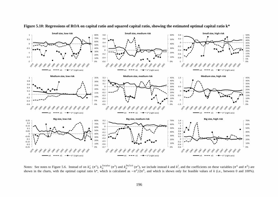
196
Figure 5.10: Regressions of ROA on capital ratio and squared capital ratio, showing the estimated optimal capital ratio k*
Notes: See notes to Figure 5.6. Instead of on 𝑘𝑖𝑡∗ (𝜋1), 𝑘𝑖𝑡
𝑆𝑢𝑟𝑝𝑙𝑢𝑠(𝜋3) and 𝑘𝑖𝑡
𝐷𝑒𝑓𝑖𝑐𝑖𝑡(𝜋2), we include instead k and k
2, and the coefficients on these variables (𝜋4 and 𝜋5) are
shown in the charts, with the optimal capital ratio k*, which is calculated as −𝜋4/2𝜋5, and which is shown only for feasible values of k (i.e., between 0 and 100%).
0%
10%
20%
30%
40%
50%
60%
70%
80%
-2
-1.5
-1
-0.5
0
0.5
1Small size, low risk
π4 π5 k* (right axis)
0%
10%
20%
30%
40%
50%
60%
-0.6
-0.4
-0.2
0
0.2
0.4
0.6
0.8Small size, medium risk
π4 π5 k* (right axis)
0%
5%
10%
15%
20%
25%
30%
35%
40%
45%
50%
-1
-0.8
-0.6
-0.4
-0.2
0
0.2
0.4Small size, high risk
π4 π5 k* (right axis)
0%
5%
10%
15%
20%
25%
30%
35%
-0.6
-0.4
-0.2
0
0.2
0.4
0.6
0.8
1Medium size, low risk
π4 π5 k* (right axis)
0%
5%
10%
15%
20%
25%
30%
35%
40%
45%
-0.6
-0.5
-0.4
-0.3
-0.2
-0.1
0
0.1
0.2
0.3Medium size, medium risk
π4 π5 k* (right axis)
0%
5%
10%
15%
20%
25%
30%
35%
40%
45%
-1.5
-1
-0.5
0
0.5
1
1.5Medium size, high risk
π4 π5 k* (right axis)
0%
10%
20%
30%
40%
50%
60%
70%
80%
-0.25
-0.2
-0.15
-0.1
-0.05
0
0.05
0.1
0.15
0.2
0.25Big size, low risk
π4 π5 k* (right axis)
0%
10%
20%
30%
40%
50%
60%
70%
-0.7
-0.6
-0.5
-0.4
-0.3
-0.2
-0.1
0
0.1
0.2Big size, medium risk
π4 π5 k* (right axis)
0%
10%
20%
30%
40%
50%
60%
70%
-0.6
-0.4
-0.2
0
0.2
0.4
0.6
0.8
1
1.2
1.4Big size, high risk
π4 π5 k* (right axis)
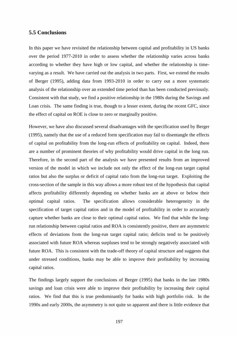
197
5.5 Conclusions
In this paper we have revisited the relationship between capital and profitability in US banks
over the period 1977-2010 in order to assess whether the relationship varies across banks
according to whether they have high or low capital, and whether the relationship is time-
varying as a result. We have carried out the analysis in two parts. First, we extend the results
of Berger (1995), adding data from 1993-2010 in order to carry out a more systematic
analysis of the relationship over an extended time period than has been conducted previously.
Consistent with that study, we find a positive relationship in the 1980s during the Savings and
Loan crisis. The same finding is true, though to a lesser extent, during the recent GFC, since
the effect of capital on ROE is close to zero or marginally positive.
However, we have also discussed several disadvantages with the specification used by Berger
(1995), namely that the use of a reduced form specification may fail to disentangle the effects
of capital on profitability from the long-run effects of profitability on capital. Indeed, there
are a number of prominent theories of why profitability would drive capital in the long run.
Therefore, in the second part of the analysis we have presented results from an improved
version of the model in which we include not only the effect of the long-run target capital
ratios but also the surplus or deficit of capital ratio from the long-run target. Exploiting the
cross-section of the sample in this way allows a more robust test of the hypothesis that capital
affects profitability differently depending on whether banks are at above or below their
optimal capital ratios. The specification allows considerable heterogeneity in the
specification of target capital ratios and in the model of profitability in order to accurately
capture whether banks are close to their optimal capital ratios. We find that while the long-
run relationship between capital ratios and ROA is consistently positive, there are asymmetric
effects of deviations from the long-run target capital ratio; deficits tend to be positively
associated with future ROA whereas surpluses tend to be strongly negatively associated with
future ROA. This is consistent with the trade-off theory of capital structure and suggests that
under stressed conditions, banks may be able to improve their profitability by increasing
capital ratios.
The findings largely support the conclusions of Berger (1995) that banks in the late 1980s
savings and loan crisis were able to improve their profitability by increasing their capital
ratios. We find that this is true predominantly for banks with high portfolio risk. In the
1990s and early 2000s, the asymmetry is not quite so apparent and there is little evidence that

198
low capital banks were able to improve profitability by raising capital ratios. This stands in
contrast to the observation that capital ratios were rising rapidly over this time period, often
well in excess of capital requirements (Flannery and Rangan 2008, Berger et al 2008). While
studies such as Flannery and Rangan (2008) have argued that increased market discipline
played a role in the rise in capital ratios, our findings suggest instead that this is not the case;
indeed market discipline seems to have supported reductions in capital requirements for those
banks with high capital relative to their long-run targets. With respect to the recent crisis
period, there is a stark contrast between the findings from the model based on Berger (1995)
and the improved model, since while the basic model finds that increasing capital drives
(Granger causes) an increase in ROA in this period, the improved model does not suggest that
low capital banks were able to improve ROA by raising capital ratios. Again we find a strong
negative relationship for banks with high capital relative to their long-run target capital ratios.
These results may reflect the role of official support in softening the effect of market
discipline.
These results have important policy implications for the operation of capital requirements.
The cost of capital requirements depends on where they are set relative to banks‘ own desired
level of capital. As we have shown, banks tend to have a desired level of capital above which
increases in capital may reduce profitability. Capital requirements, if they are binding, are
likely to have a larger effect on banks‘ costs the higher above the optimal capital ratio they
are set. Since the optimal capital ratio is likely to vary over financial cycles, the costs of
capital requirements will vary as well, which is a factor that has not been taken into account
in most assessments of the impact of capital requirements. This is particularly relevant for
macroprudential policy. This policy operates through a regime of time-varying capital
requirements, which rise during booms and fall during busts in order to smooth banks‘ credit
supply over the cycle. If optimal capital requirements rise during a crisis, it is unlikely that
banks will have incentives to reduce their capital ratios if capital requirements are cut. This
may limit the effectiveness of counter-cyclical capital requirements, since reductions in the
capital requirement will have little effect on banks whose optimal capital ratios meet or
exceed the level of the capital requirement. On the other hand, increases in capital
requirements during a boom period may raise a bank‘s capital ratio above the desired level,
consistent with the aims of the policy.
199
Chapter 6 : Conclusion
This thesis has presented the findings of three related research studies related to the role of
bank capital in banks‘ behaviour and adjustment of their balance sheets. Here we do not
repeat the detailed findings of each of those chapters here (since each chapter has its own
conclusions), but it may be useful to list what should be regarded as the key findings:
The research is strongly supportive of the existence of a long-run target capital ratio
for US and UK banks which has a strong influence of banks‘ balance sheet
management.
Whether market and regulatory targets are binding on banks is likely to vary over
banks and time periods, and we have identified that in the UK in the pre-crisis period
(1996-2007) supervisory discretionary add-ons had a significant role in the
determination of banks‘ own capital targets. In this period, banks can be observed to
vary their total capital and assets in order to maintain their desired buffer relative to
the regulatory minimum.
Theory tells us that the optimal capital ratio for each bank is likely to be cyclical,
and we find evidence consistent with this in two separate studies: one of large UK
banks‘ lending rates (Chapter 4) and one of US banks‘ profitability (Chapter 5).
These findings suggest that, in periods of banking sector distress, the relationship
between capital and bank performance may alter so that banks can reduce costs and
margins and profitability by increasing capital ratios. The benefits may be passed on
to customers in the form of lower lending rates, or to investors in the form of higher
profits.
As we have argued throughout the thesis, these findings are highly relevant to the design and
calibration of regulatory capital standards. We argue there are three separate policy
implications:
Our finding that, in the pre-crisis period, banks tended to meet capital targets by
adjusting their risk-weighted assets and altering the level of low-quality, tier 2 capital,
suggests that banks tend to take the lowest cost way to meet capital standards. These
results provide support for the proposals in the Basel III agreement to tighten the

200
definition of capital and require banks to hold sufficient quantities of high-quality,
loss absorbing capital (e.g. core tier 1).
Our results are consistent with the idea that banks‘ own optimal capital ratios tend to
be highly cyclical, which offers lessons for impact assessment of introducing higher
capital requirements such as those proposed by Basel III. Most impact assessment
exercises have assumed the relationship between capital and the cost of
intermediation to be fixed over the cycle and based on long-run estimates of the gap
between the return on equity and debt. Our findings, based on indirect inference from
lending rates and profitability of banks, suggest that these studies offer a misleading
estimate of the short-run effects of higher capital standards. The relationship in fact
moves with the cycle, meaning that in periods of banking sector distress the
incremental costs of capital requirements are much lower than they are under more
normal conditions.
These findings also have implications for counter-cyclical capital requirements, which
are intended to smooth credit cycles by stimulating lending in bad times and
constraining in good times. Our findings suggest that the impact of reductions in
capital requirements during a crisis may be muted if banks‘ own optimal capital ratios
rise during a crisis. Therefore, very substantial counter-cyclical variations in capital
requirements (i.e. large increases during booms and large reductions in a downturn)
may be necessary in order to achieve the aim of stimulating credit supply in such
conditions. The policy is more likely to be successful during boom periods, when
capital requirements tend to rise and banks‘ optimal capital ratios tend to fall.
Finally, we offer suggestions on future research which could be done to extend the findings in
the thesis:
First, in Chapter 4 we examined the long-run and short-run effects of bank capital on
lending rates, but we noted that the short-run effects were ambiguous in sign (see
section 4.3.2). Briefly, the short-run relationship may be positive if banks are raising
interest rate and raising capital ratios at the same time, but unexpected shocks to the
capital ratio could induce a negative relationship since a downward shock causes
banks to raise interest rates in response. Further examination of this issue would aid
our understanding of how banks respond to exogenous capital shocks, such as
changes in capital requirements. A possible strategy would be to estimate

201
simultaneous equations for bank capital ratios and lending rates, identifying the two
effects above by using lags. The first, positive effect, should be picked up by a
positive sign on lagged interest rates in the capital ratio equation, whereas the second,
negative, relationship should be picked up by a negative sign on lagged capital ratios
in the interest rate equation.
Second, in Chapter 5 we extended the model of Berger (1995) to address a number of
problems, but one aspect we have not covered in detail is the role of capital
requirements. Put simply, capital requirements should result in important variations
in the ―trade-off‖ story we have outlined, since banks are punished by the market
and/or regulators for falling close to or below the capital requirement. The effects we
have observed are based on banks‘ own capital targets, which are generated either by
internal incentives or by capital requirements (or, most likely, some combination of
the two). An interesting extension would be to look at how the long-run and short-run
relationships vary when the bank falls close to the regulatory capital minimum by
using interaction effects. This would require using data on bank holding companies
rather than individual banks, since the data on risk-weighted assets (on which capital
requirements are based under the Basel regimes) are only available for the former.
Third, while we have been careful to control for time-specific macroeconomic effects
in all three papers, we have not examined how the relationship between bank capital
and lending behaviour interacts with the operation of monetary policy. According to
the conventional bank lending channel, bank capital can have an important effect
exacerbating the effect of monetary policy changes, although, as we noted in Chapter
2, this view has its critics. The exceptional monetary policy employed by central
banks during the crisis may offer a useful testing ground for examining these
questions using the cross-sectional dimension of our datasets.

202
This page is intentionally left blank.
203
References
Admati, A., DeMarzo, P., Hellwig, M. and Pfleiderer, P. (2010) Fallacies, Irrelevant Facts,
and Myths in the Discussions of Capital Regulation: Why Bank Equity is Not Expensive,
Stanford Graduate School of Business Research Paper No. 2065.
Alfon, I., Argimon, I., Bascunana-Ambros, P. (2004) What determines how much capital is
held by UK banks and building societies?. FSA Occasional Paper no. 22.
Allen, B., DeYoung, R., Flannery, M., Lan, D., and Özde, Ö. (2008) How do large banking
organizations manage their capital ratios? Journal of Financial Services Research, 34, 123-
149.
Allen, F., Carletti, E. and Marquez, R. (2011) Credit market competition and capital
regulation. Review of Financial Studies, 24, 983-1018.
Altman, E. I., and Saunders, A. (2001). An analysis and critique of the BIS proposal on
capital adequacy and ratings. Journal of Banking and Finance, 25, 25-46.
Altunbaş, Y., Fazylov, O., and Molyneux, P. (2002). Evidence on the bank lending channel in
Europe. Journal of Banking and Finance, 26, 2093-2110.
Angbazo, L. (1997) Commercial bank net interest margins, default risk, interest rate risk, and
off-balance sheet banking. Journal of Banking and Finance, 21, 55-87.
Avraham, D., Selvaggi, P. and Vickery, J. I. (2012) A Structural View of U.S. Bank Holding
Companies. Federal Reserve Bank of New York Economic Policy Review, 18, 65-81.
Ayuso, J., Pérez, D., and Saurina, J. (2004). Are capital buffers pro-cyclical?: Evidence from
Spanish panel data. Journal of Financial Intermediation, 13, 249-264.
Bank of England. (2011) Instruments of Macroprudential Policy. Discussion Paper,
December.
Barajas, A., Chami, R. and Cosimano, T. (2005) Did the Basel Accord Cause a Credit
Slowdown in Latin America?, IMF Working Paper, no. 38.
Barrell, R., Davis, E. Philip, Fic, T., Holland, D., Kirby, S. and Liadze, I. (2009) Optimal
regulation of bank capital and liquidity: How to calibrate new international standards, FSA
Occasional Paper, No. 38.
204
Barrios, V. E., and Blanco, J. M. (2003). The effectiveness of bank capital adequacy
regulation: A theoretical and empirical approach. Journal of Banking and Finance, 27, 1935-
1958.
Basel Committee on Banking Supervision. (2010) Calibrating regulatory minimum capital
requirements and capital buffers: A top-down approach, October.
Berger, A. N. (1995) The relationship between capital and earnings in banking, Journal of
Money Credit and Banking 27, 432-456.
Berger, A. and Bouwman, C. (2012). Bank Capital, Survival, and Performance around
Financial Crises. Working paper, available at SSRN no. 1739089.
Berger, A., Davies, S., and Flannery, M. (2000) Comparing Market and Supervisory
Assessments of Bank Performance: Who Knows What When? Journal of Money, Credit and
Banking, 32, 641-667.
Berger, A, Demsetz, R., and Strahan, P. (1999) The consolidation of the financial services
industry: Causes, consequences, and implications for the future.
Journal of Banking and Finance, 23, 135-194.
Berger, A., DeYoung, R., Flannery, M., Lee, D. and Öztekin, Ö. (2008). How do large
banking organisations manage their capital ratios? Journal of Financial Services Research,
34, 123-149.
Berger, A. N., Herring, R. and Szegö, G. (1995) The role of capital in financial institutions,
Journal of Banking and Finance, 19, 393-430.
Berger, A. N., and Udell, G. F. (1994). Did risk-based capital allocate bank credit and cause a
credit crunch in the United States? Journal of Money, Credit and Banking, 26, 585-628.
Bernanke, B. S., and Blinder, A. S. (1988). Credit, money, and aggregate demand. The
American Economic Review, 78, 435-439.
Bernanke B., Gertler, M., Gilchrist, S. (1999) The financial accelerator in a quantitative
business cycle framework. In: Taylor, J.B., Woodford, M. (Eds.), Handbook of
Macroeconomics, Vol. 1. North-Holland: Amsterdam.
Bernanke, B. S., Lown, C. S., and Friedman, B. M. (1991). The credit crunch. Brookings
Papers on Economic Activity, 205-247.
205
Berrospide, J. and Edge, R. (2010) The effects of bank capital on lending: What do we know,
and what does it mean?, International Journal of Central Banking, December.
Best, R. and Zhang, H.. (1993) Alternative Information Sources and the Information Content
of Bank Loans, Journal of Finance, 1993, 48.
Bhattacharya, S. (1982) Aspects of monetary and banking theory and moral hazard. Journal
of Finance, 37, 371–384.
Bhattacharya, S., Plank, M., Strobl, G. and Zechner, J. (2002) Bank capital regulation with
random audits. Journal of economic dynamics and control, 26, 1301-1321.
Bhattacharya, S. and Thakor, A. (1993) Contemporary banking theory. Journal of Financial
Intermediation 3, 2–50.
Blum, J., and Hellwig, M. (1995). The macroeconomic implications of capital adequacy
requirements for banks. European Economic Review, 39, 739-749.
Blum, D. and Nakane, M. (2006), The Impact of Capital Requirements in Brazilian Banks
Loan Supply, Banco Central de Brazil, Relatürio de Economia Bancária e Crédito.
Blundell, R. and Stephen B. (1998) Initial conditions and moment restrictions in dynamic
panel data models. Journal of Econometrics, 87, 115-43.
Boot, A., Greenbaum, S. and Thakor, A., (1993) Reputation and discretion in financial
contracting, The American Economic Review, 83, pages 1165-83.
Brana, S. and Lahet, D. (2009): Capital requirement and financial crisis: the case of Japan
and the 1997 Asian crisis, Japan and the World Economy, 21, 97–104.
Brealey, R., Myers, S. and Allen, F. (2010) Principles of Corporate Finance, McGraw-
Hill/Urwin.
Brinkmann, E. J., and Horvitz, P. M. (1995). Risk-based capital standards and the credit
crunch. Journal of Money, Credit and Banking, 27, 848-863.
Brun-Aguerre, R., Fuertes, A.-M., and Phylaktis, K. (2011) Country and Time Variation in
Exchange Rate Pass-Through: What Drives It? Forthcoming in Journal of International
Money and Finance.
Brunnermeier, M. (2009) Deciphering the liquidity and credit crunch 2007-2008, Journal of
Economic Perspectives 23, 77-100.

206
Brunnermeier, M., Sannikov, Y. (2011) A macroeconomic model with a financial sector.
Working paper, Princeton.
Bruno, G. S. F. (2005) Approximating the Bias of the LSDV Estimator for Dynamic
Unbalanced Panel Data Models, Economics Letters 87, 361-366.
Bun, M. J. G. and Kiviet, J. F. (2003) On the diminishing returns of higher order terms in
asymptotic expansions of bias, Economics Letters 79, 145–152.
Buser, Stephen, Andrew Chen and Edward Kane. (1981) Federal Deposit Insurance,
Regulatory Policy, and Optimal Bank Capital. The Journal of Finance, 35, 51-60.
Button, R., Pezzini, S. and Rossiter, N. (2010) Understanding the price of new lending to
households, Bank of England Quarterly Bulletin, No. 10-03.
Carbó-Valverde, S. and Rodríguez-Fernández, F. (2007) The determinants of bank margins in
European banking, Journal of Banking and Finance, 31, 2043-2063.
Carlstrom, C. and Samolyk, K. (1995). Loan sales as a response to market-based capital
constraints. Journal of Banking and Finance, 19, 627-646.
Cornett, M., McNutt, J., Strahan, P. and Tehranian, H. (2011) Liquidity risk management and
credit supply in the financial crisis, Journal of Financial Economics, 101, 297-312.
Covitz, D., Hancock, D., and Kwast, M. (2004) A reconsideration of the risk sensitivity of
US banking organization subordinated debt spreads: A sample selection approach. Federal
Reserve Bank of New York Economic Policy Review, 10, 73–95.
Demirgüc-Kunt, A. and Huizinga, H. (1999) Determinants of commercial bank interest
margins and profitability: Some international evidence, The World Bank Economic Review
13, 379-408.
Demsetz, R., Saidenberg, M., and Strahan, P. (1996) Banks with something to lose: the
disciplinary role of franchise value. Federal Reserve Bank of New York Economic Policy
Review, 2, 1–14.
DeYoung, R. (2010) Banking in the United States. In Allen N. Berger, Philip Molyneux, and
John O. Wilson (eds.), Oxford Handbook of Banking. Oxford University Press.
DeYoung, R., Flannery, M., Lang, W. and Sorescu, S. (2001) The Information Content of
Bank Exam Ratings and Subordinated Debt Prices. Journal of Money, Credit, and Banking,
33, 900-925.
207
Diamond, D. (1984) Financial intermediation and delegated monitoring, Review of Economic
Studies, 51, 393-414.
Diamond D. W. and Dybvig P.H. (1983) Bank runs, deposit insurance, and liquidity. Journal
of Political Economy, 91, 401–419.
Diamond, D. W., and Rajan, R. G. (2000). A theory of bank capital. The Journal of Finance,
55, 2431-2465.
Disyatat, P. (2008) Monetary policy implementation: Misconceptions and their consequences,
Bank for International Settlements, working paper no. 269.
Ediz, T., Michael, I., and Perraudin, W. (1998). The impact of capital requirements on UK
bank behaviour. Economic Policy Review, 4.
Elliott, D. (2009) Quantifying the effects on lending of increased capital requirements, Pew
Financial Reform Project Briefing, No. 7.
Ellis, D. and Flannery, M. (1992) Does the debt market assess large banks‘ risk?: Time series
evidence from money center CDs, Journal of Monetary Economics, 20, 481-502.
Estrella, A. (2004) The Cyclical Behavior of Optimal Bank Capital, Journal of Banking and
Finance 28, 1469-1498.
Fama, E. F. (1978) The Effects of a Firm's Financing and Investment Decisions on the
Welfare of its Security Holders. American Economic Review, 68, 272-284.
Fama, E. F., and French, K. R. (1998) Taxes, financing decisions and firm value, The Journal
of Finance, 53, 819-843.
Fama, E. F., and French, K. R. (2002). Testing trade-off and pecking order predictions about
dividends and debt. The Review of Financial Studies, 15(1), 1-33.
Financial Services Authority (2006) Strengthening Capital Standards 2, Consultation Paper
No. 06-03.
Fischer, M., Mattes, J. and Steffen, S. (2011) Bank Capital, Competition and Loan Spreads,
unpublished working paper, ESMT European School of Management and Technology,
Berlin, available at SSRN: http://ssrn.com/abstract=1483717.
Flannery, M. (1998). Using market information in bank prudential supervision: A review of
the UK empirical evidence. Journal of Money, Credit and Banking, 30, 273-305.
208
Flannery, M.J. and Hankins, K. (2012) Estimating dynamic panel models incorporate finance.
Available at: http://papers.ssrn.com/sol3/papers.cfm?abstract_id=1108684.
Flannery, M. J. and Rangan K. P. (2006) Partial adjustment toward target capital structures,
Journal of Financial Economics, 79, 469-506.
Flannery, M. J., and Rangan, K. P. (2008). What caused the bank capital build-up of the
1990s?, Review of Finance, 12, 391.
Flannery, M. and Sorescu, S. (1996). Evidence of Bank Market Discipline in Subordinated
Debenture Yields: 1983-1991. The Journal of Finance, 51, 1347-1377
Francis, W. and Osborne, M. (2009) Bank regulation, capital and credit supply: Measuring
the impact of prudential standards, FSA Occasional Paper, no. 31.
Francis, W. and Osborne, M. (2010) On the Behavior and Determinants of Risk‐Based
Capital Ratios: Revisiting the Evidence from UK Banking Institutions. International Review
of Finance, 10, 485-518.
Francis, W. and Osborne, M. (2012) Capital requirements and bank behavior in the UK: Are
there lessons for international capital standards?, Journal of Banking and Finance, 36, 803-
816
Frank, M. and Goyal, V. (2003). Testing the pecking order theory of capital structure,
Journal of Financial Economics, 67, 217-248.
Frank, M. and Goyal, V. (2008) Trade-off and pecking order theories of debt, in: E. Eckbo
(ed.), Handbook of Corporate Finance: Empirical Corporate Finance, Vol. 2, Elsevier,
Amsterdam, pp. 135–202.
Freixas, X., and Rochet, J.-C. (2008). Microeconomics of banking, 2nd edition, The MIT
Press.
Fuertes, A.-M. and Heffernan, S. (2009) Interest rate transmission in the UK: A comparative
analysis across financial firms and products, International Journal of Finance and Economics
14, 45-63.
Fuertes, A.-M., Heffernan, S. and Kalotychou, E. (2010) How do UK banks react to changing
central bank rates?, Journal of Financial Services Research 37, 99-130.
Furfine, C. (2001) Bank portfolio allocation: The impact of capital requirements, regulatory
monitoring, and economic conditions. Journal of Financial Services Research 20, 33-56.
209
Gambacorta, L. and Mistrulli, P. E. (2004) Does bank capital affect lending behaviour?,
Journal of Financial Intermediation 13, 436-457.
Goddard, J., Molyneux, P. and Wilson, J. (2004). Dynamics of growth and profitability in
banking. Journal of Money, Credit and Banking, 36, 1069-1090.
Goodhart, C., Hofmann, B., and Segoviano, M. (2004). Bank regulation and macroeconomic
fluctuations. Oxford Review of Economic Policy, 20(4), 591.
Gordy, M., Howells, B. (2006) Procyclicality in Basel II: Can we treat the disease without
killing the patient?. Journal of Financial Intermediation 15, 395–417.
Graham, J. (2000) How big are the tax benefits of debt? The Journal of Finance, 55, 1901-
1941.
Gropp, R. and Heider, F. (2010) The Determinants of Bank Capital Structure. Review of
Finance, 14, 587–622 .
Gropp, R., Vesala, J. and Vulpes, G. (2006) Equity and bond market signals as leading
indicators of bank fragility. Journal of Money, Credit and Banking, 38, 399-428.
Hadlock, C. and James, C. (2002) Do banks provide financial slack? The Journal of Finance,
57, 1383-1419.
Hancock, D., Laing, A., Wilcox, J. (1995) Bank capital shocks: Dynamic effects on
securities, loans and capital. Journal of Banking and Finance 19, 661-677.
Hanson, S., Stein, J. and Kashyap, A. (2010) A macroprudential approach to financial
regulation, Journal of Economic Perspectives 25, 3-28.
Hancock, D., Wilcox, J. (1994) Bank capital and credit crunch: The roles of risk-weighted
and unweighted capital regulations. Journal of the American Real Estate and Urban
Economics Association 22, 59-91.
Harris, M. and Raviv, A. (1991) The theory of capital structure, The Journal of Finance, 46,
297–356.
Heffernan, S. (2002). How do UK financial institutions really price their banking products?
Journal of Banking and Finance, 26, 1997-2016.
Heffernan, S. (2006). UK bank services for small business: How competitive is the market?
Journal of Banking and Finance, 30, 3087-3110.
210
Heid, F. (2007). The cyclical effects of the Basel II capital requirements. Journal of Banking
and Finance, 31, 3885-3900.
Hellmann, T., Murdoch, K., and Stiglitz, J. (2000) Liberalization, Moral Hazard in Banking,
and Prudential Regulation: Are Capital Requirements Enough? American Economic Review,
90, 147-165.
Ho, T. S. Y., and Saunders, A. (1981). The determinants of bank interest margins: Theory
and empirical evidence. The Journal of Financial and Quantitative Analysis, 16, 581-600.
Holmstrom, B. and Tirole, J. (1997) Financial intermediation, loanable funds, and the real
sector, Quarterly Journal of Economics, 112, 663-691.
Honda, Y. (2002). The effects of the Basle accord on bank credit: The case of Japan. Applied
Economics, 34(10), 1233.
Huang, Z. (2003). Evidence of a bank lending channel in the UK. Journal of Banking and
Finance, 27, 491-510.
Hubbard, R.G., Kuttner, K. and Palia, D. (2002) Are there bank effects in borrowers‘ cost of
funds?, Journal of Business, 75, 559-581.
Institute of International Finance, (2010) Cumulative Impact on the Global Economy of
Proposed Changes in the Banking Regulatory Framework, June.
Jackson, P., Furfine, C., Groeneveld, H., Hancock, D., Jones, D., Perraudin, W. (1999)
Capital requirements and bank behaviour: The impact of the Basle accord, Basle Committee
on Banking Supervision Working Paper No. 1.
Jacques, K. and Nigro, P., (1997) Risk-based capital, portfolio risk, and bank capital: A
simultaneous equations approach, Journal of Economics and Business, 49, 533-547.
Jagtiani, J., George K., and Lemieux, C. (2002) The effect of credit risk on bank and bank
holding company bond yields: evidence from the post-FDICIA period. The Journal of
Financial Research, 25, 559–575.
James, C. (1987). Some evidence on the uniqueness of bank loans. Journal of Financial
Economics, 19, 217-235.
Jayaratne, J. and Morgan, D. (2000) Capital market frictions and deposit constraints at banks,
Journal of Money, Credit and Banking, 32, 74-92.
211
Jensen, M. (1986) Agency costs of free cash flow, corporate finance, and takeovers, The
American Economic Review, 76, 323-329
Jensen, M. C. and Meckling, W. H. (1976) Theory of the Firm: Managerial Behavior, Agency
Costs and Ownership Structure, Journal of Financial Economics, 3, 305–360.
Jokipii, T. (2009) Nonlinearity of bank capital and charter values. Swiss National Bank
working paper.
Jokipii, T. and Milne, A. (2011) Bank capital buffer and risk adjustment decisions. Journal of
Financial Stability, 7, 165-178.
Judson, R. and Owen, A. (1999) Estimating Dynamic Panel Data Models: A Practical Guide
for Macroeconomists, Economics Letters, 65, 9-15.
Kashyap, A. K., and Stein, J. C. (1995). The impact of monetary policy on bank balance
sheets. Carnegie-Rochester Conference Series on Public Policy, 42, 151-195.
Kashyap, A. K., and Stein, J. C. (2000). What do a million observations on banks say about
the transmission of monetary policy? American Economic Review, 90, 407-428.
Kashyap, A. K., and Stein, J. C. (2004) Cyclical implications of the Basel II capital standards,
Federal Reserve Bank of Chicago, Economic Perspectives, Q1
Kashyap, A. K., Stein, J. C., and Wilcox, D. W. (1993). Monetary policy and credit
conditions: Evidence from the composition of external finance. The American Economic
Review, 83, 78-98.
Kashyap, A., Stein, J. and Hanson, S. (2010) An Analysis of the Impact of ‗Substantially
Heightened‘ Capital Requirements on Large Financial Institutions, unpublished working
paper, Harvard University.
Keeley, M. (1990) Deposit insurance, risk, and market power in banking. American
Economic Review 80, 1183-1200.
Kim, D., and Santomero, A. M. (1988) Risk in banking and capital regulation. The Journal of
Finance, 43, 1219-1233.
Kishan, R. P., and Opiela, T. P. (2000) Bank size, bank capital, and the bank lending channel.
Journal of Money, Credit and Banking, 32, 121-141.
Kishan, R. P., and Opiela, T. P. (2006) Bank capital and loan asymmetry in the transmission
of monetary policy. Journal of Banking and Finance, 30, 259-285.

212
Kwan, S. and Eisenbeis, R. (1997) Bank Risk, Capitalization, and Operating Efficiency,
Journal of Financial Services Research, 12, 117-131.
Leland, H. and Pyle, H. (1977) Informational Asymmetries, Financial Structure, and
Financial Intermediation, Journal of Finance, 32, 371-387.
Lindquist, K.-G. (2003) Banks‘ buffer capital: How important is risk? Norges Bank working
paper 2003:11.
Lo, A. (2012) Reading About the Financial Crisis: A 21-Book Review, Forthcoming in
Journal of Economic Literature.
Lummer, Scott and John McConnell (1989) Further Evidence on the Bank Lending Process
and the Capital Market Response to Bank Loan Agreements, Journal of Financial
Economics, 1989, 25.
Marcus, A. (1984) Deregulation and bank financial policy, Journal of Banking and Finance
8, 557-565.
McGuire, P., Tarashev, N. (2008) Global monitoring with the BIS international banking
statistics. Bank for International Settlements Working Paper, No. 244.
Mehran, H. and Thakor, A. (2011) Bank Capital and Value in the Cross Section, Review of
Financial Studies, 24, 1019-1067.
Memmel, C. and Raupach, P. (2007), How Do Banks Adjust Their Capital Ratios? Evidence
from Germany, Discussion Paper Series 2: Banking and Financial Studies 2007:06,
Deutsche Bundesbank, Research Centre.
Merrouche, O. and Nier, E. (2011). What Caused the Global Financial Crisis?—Evidence on
the Drivers of Financial Imbalances 1999–2007. IMF Working Paper 10/ 265, December.
Merton, R., (1974) On the Pricing of Corporate Debt: the Risk Structure of Interest Rates,
The Journal of Finance 29, 449-470.
Merton, R. (1977) An analytic derivation of the cost of deposit insurance and loan guarantees
an application of modern option pricing theory. Journal of Banking and Finance, 1, 3-11.
Merton, Robert. (1978) On the cost of deposit insurance when there are surveillance costs.
The Journal of Business, 51, 439-452.
Miles, D., Yang, J. and Marcheggiano, G. (2011) Optimal Bank Capital, External Monetary
Policy Committee Unit, Bank of England Discussion Papers, No. 31.

213
Miller, M. (1977). Debt and taxes. The Journal of Finance, 32, Papers and Proceedings of the
Thirty-Fifth Annual Meeting of the American Finance Association, Atlantic City, New
Jersey, September 16-18, 1976, 261-275.
Miller, M. (1989). The Modigliani-Miller propositions after thirty years. Journal of Applied
Corporate Finance, 2, 6-18.
Miller, M. (1995) Do the MandM propositions apply to banks? Journal of Banking and
Finance, 19, 483–489.
Milne, A. (2004) The inventory perspective on bank capital, unpublished working paper,
Cass Business School City University, London, available at SSRN:
http://ssrn.com/abstract=576062.
Milne, A. (2009) Macroprudential Policy: What can it achieve? Oxford Review of Economic
Policy, 25, 608-629
Milne, A. and Onorato, M. (2010), Risk-adjusted measures of value creation in financial
institutions, European Financial Management, 18
Milne, A. and Whalley, E. (2002) Bank capital and incentives for risk-taking, unpublished
working paper, available at SSRN: http://ssrn.com/abstract =303176.
Milne, A., and Wood, G. (2009) The bank lending channel reconsidered, Bank of Finland
working paper.
Modigliani, F. and Miller, M. (1958) The Cost of Capital, Corporation Finance and the
Theory of Investment, American Economic Review 48, 261-297.
Morgan, D. and Stiroh, K. (2001) Market discipline of banks: The asset test. Journal of
Financial Services Research, 20, 195-208.
Myers, S. (1977) Determinants of Corporate Borrowing, Journal of Financial Economics, 5,
147-75.
Myers, S. (1984) The capital structure puzzle, The Journal of Finance, 39, 575-592
Myers, S. (2001) Capital structure, Journal of Economic Perspectives 15, 81-102.
Myers, S. and Majluf, N. (1984) Corporate financing and investment decisions when firms
have information that investors do not have, Journal of Financial Economics, 13, 187-221.

214
Nier, E. and Ursel B. (2006) Market discipline, disclosure and moral hazard in banking.
Journal of Financial Intermediation, 15, 332-361.
Nier, E., Zicchino, L., (2005) Bank weakness and loan supply. Bank of England Financial
Stability Review, December, 85-93.
O‘Hara, M. and Shaw, W. (1990) Deposit insurance and wealth effects: the value of being
‗too big to fail‘. The Journal of Finance, 45, 1587–1600.
Oliner, S. D., and Rudebusch, G. D. (1996a). Is there a broad credit channel for monetary
policy? Economic Review-Federal Reserve Bank of San Francisco, , 3-13.
Oliner, S. D., and Rudebusch, G. D. (1996b). Monetary policy and credit conditions:
Evidence from the composition of external finance: Comment. The American Economic
Review, 86, 300-309.
Osterberg, W. and Thomson, J. (1996) Optimal financial structure and bank capital
requirements: an empirical investigation. Journal of Financial Services Research, 10, 315–
332.
Peek, J., and Rosengren, E. (1995). The capital crunch: Neither a borrower nor a lender be.
Journal of Money, Credit and Banking, 27, 625-638.
Peek, J., and Rosengren, E. (2000) Collateral damage: Effects of the Japanese bank crisis on
real activity in the United States, American Economic Review, 95, 1144-1166.
Peura, S. and Keppo, J. (2006) Optimal bank capital with costly recapitalization, Journal of
Business, 79, 2162–2201.
Rajan, R. (1992) Insiders and outsiders: The choice between informed and arm's-length debt.
The Journal of Finance, 47, 1367-1400.
Rajan, R. and Zingales, L. (1995) What do we know about capital structure? Some evidence
from international data, The Journal of Finance, 50, 1421-1460.
Repullo, R., Saurina., J., Trucharte, C., (2010) Mitigating the pro-cyclicality of Basel II.
Economic Policy 25:64, 259-702.
Repullo, R., and Suarez, J. (2004). Loan pricing under Basel capital requirements. Journal of
Financial Intermediation, 13, 496-521.
Repullo, R., and Suarez, J. (2008). The procyclical effects of Basel II. Centre for Economic
Policy Research Discussion Paper no. 6862.
215
Rochet, J.-C. (1992) Capital requirements and the behaviour of commercial banks. European
Economic Review, 36, 1137-1178.
Roodman, D. (2009) How to do xtabond2: An introduction to difference and system GMM in
Stata. Stata Journal, 9, 86-136.
Santos, J. and Winton, A. (2010) Bank Capital, Borrower Power, and Loan Rates,
unpublished working paper, AFA 2010 Atlanta Meetings Paper, available at SSRN:
http://ssrn.com/abstract =1343897.
Saunders, A. and Schumacher, L. (2000) The determinants of bank interest rate margins: An
international study, Journal of International Money and Finance, 19, 813-832.
Sharpe, S. A. (1990) Asymmetric information, bank lending, and implicit contracts: A
stylized model of customer relationships. The Journal of Finance, 45, 1069-87.
Sharpe, S. (1995) Bank capitalization, regulation, and the credit crunch: A critical review of
the research findings. Board of Governors of the Federal Reserve System Finance and
Economics Discussion Series, No. 95:20.
Shrieves, R. E., and Dahl, D. (1995) Regulation, recession, and bank lending behavior: The
1990 credit crunch. Journal of Financial Services Research, 9, 5-30.
Shyam-Sunder, L. and Myers, S. (1999) Testing static trade-off against pecking order models
of capital structure, Journal of Financial Economics, 51, 219-244.
Sironi, A. (2003) Testing for Market Discipline in the European Banking Industry: Evidence
from Subordinated Debt Issues. Journal of Money, Credit, and Banking, 35, 443-472.
Stein, J. (1998) An adverse-selection model of bank asset and liability management with
implications for the transmission of monetary policy, RAND Journal of Economics 29, 466-
486.
Stiglitz, J. (1974) On the irrelevance of corporate financial policy. American Economic
Review, 64, 851-866.
Stolz, S. (2007) Bank Capital and Risk-taking: The Impact of Capital Regulation, Charter
Value, and the Business Cycle, Kiel Studies no. 337, Kiel Institute for the World Economy.
Swank, J. (1996) Theories of the Banking Firm: A Review of the Literature, Bulletin of
Economic Research, 48, 173-207.

216
Thakor, A. V. (1996) Capital requirements, monetary policy, and aggregate bank lending:
Theory and empirical evidence, The Journal of Finance, 51, 279-324.
Van den Heuvel, S. J. (2002) The bank capital channel of monetary policy, working paper,
The Wharton School, University of Pennsylvania
VanHoose, D. (2007) Theories of bank behaviour under capital regulation, Journal of
Banking and Finance, 31, 3680-3697.
VanHoose, D. (2008), Bank Capital Regulation, Economic Stability, and Monetary Policy:
What Does the Academic Literature Tell Us?, Atlantic Economic Journal, 36, 1-14.
Vennet, R. (2002) Cost and profit efficiency of financial conglomerates and universal banks
in Europe. Journal of Money, Credit and Banking, 34, 254-282.
Wagster, J. (1999). The Basel accord of 1988 and the international credit crunch of 1989-
1992. Journal of Financial Services Research, 15, 123-143
Wahrenburg, M. and Steffen, S. (2008) Syndicated Loans, Lending Relationships and the
Business Cycle, unpublished working paper, available at SSRN:
http://ssrn.com/abstract=1101022.
Wald, J. (1999) How firm characteristics affect capital structure: An international
comparison, The Journal of Financial Services Research, 22, 161-187.
Wall, L. and Peterson, D. (1988) Capital Changes at Large Affiliated Banks. Journal of
Financial Services Research, 1, 253-275.
Windmeijer, F. (2005) A finite sample correction for the variance of linear efficient two-step
GMM estimators. Journal of Econometrics, 126, 25-51.
Woo, D. (2003). In search of capital crunch: Supply factors behind the credit slowdown in
Japan. Journal of Money, Credit and Banking, 35, 1019-1038.
Yang, J. and Tsatsaronis, K. (2012) Bank stock returns, leverage and the business cycle, Bank
for International Settlements Quarterly Review, March 2012.