Diploma thesis

Electron Spin Resonance Spectroscopy onGraphite Intercalation Compounds

Gábor Fábián

Thesis advisor: Dr. Ferenc Simonassociate professorDepartment of PhysicsInstitute of PhysicsBME

Budapest University of Technology and EconomicsBME

2011

i

Diplomatéma-kiírás

Témavezető:

Neve: Simon Ferenc

Tanszéke: Fizika Tanszék

E-mail címe: simon@esr.phy.bme.hu

Telefonszáma: 463-3816

Azonosító: DM-2010-81

Diplomatéma címe: Elektron spin rezonancia spektroszkópia szén nanocsöveken

Melyik szakiránynak ajánlott? ”Kutatófizikus”

A jelentkezővel szemben támasztott elvárások: Jeles eredményű BSc a fizikus

szakirányon.

Leírása: Az elmúlt évtized a nanoszerkezetű anyagok és azon belül is az ún. szén nanoc-

sövek kutatásának rohamos fejlődését hozta. A szén nanocsövek a szén negyedik mó-

dosulatát képviselik a grafit, gyémánt és fullerének után. A terület megoldandó tech-

nológiai problémái mellett számos alapvető kérdés, mint pl. a szén nanocsövek alapál-

lapota és Fermi felület közeli állapotsűrűsége jelenleg is intenzíven kutatott. Az MsC

diplomamunka ezen kutatásokhoz járul hozzá szintézis és szilárdtestspektroszkópia al-

kalmazásával, e két módszer kombinálásával. A munkához fontos az elméleti ismeretek-

ben, szilárdtestfizikában való biztos jártasság, előny a jó gyakorlati érzék, önállóság és a

kísérleti munkához való affinitás.

ii

Önállósági nyilatkozat

Alulírott Fábián Gábor, a Budapesti Műszaki és Gazdaságtudományi Egyetem

Fizikus mesterszak (MSc) kutatófizikus szakirányának hallgatója kijelentem, hogy ezt a

diplomamunkát meg nem engedett segítség igénybevétele nélkül, saját magam készítet-

tem. Minden olyan szövegrészt, adatot, diagramot, ábrát, vagy bármely más elemet,

melyet szó szerint vagy azonos értelemben, de átfogalmazva más forrásából vettem,

egyértelműen megjelöltem a forrás megadásával.

Budapest, 2011. június 1. Fábián Gábor

iii

Köszönetnyilvánítás

Elsőként szüleimnek tartozom köszönettel, hogy tanulmányaim során töretlenül tá-

mogattak, és bíztak bennem.

Ezúton fejezem ki hálámat témavezetőmnek, Dr. Simon Ferencnek, aki rendkívüli

lelkesedéssel vont be a kísérleti munka minden részébe, és vezetett be a kísérleti fizika

világába. Segítsége és tanácsai nélkül jelen dolgozat és eddigi eredményeim nem valósul-

hattak volna meg. Köszönöm a dolgozat többszöri alapos átnézését, és az útmutatást a

lehető legjobb diplomamunka megírásához.

Köszönöm Prof. Mihály György tanszékvezető úrnak a méréseimhez szükséges

infrastruktúra biztosítását. A tanszék mágneses rezonancia csoportjának munkatár-

sainak: Prof. Jánossy Andrásnak, Dr. Fehér Titusznak, Antal Ágnes és Karaszi Mihály

doktorandusz-hallgatóknak köszönöm, hogy lehetőséget biztosítottak a nagyfrekveciás

ESR spektrométer használatára, és segítettek kezelésében, illetve ha bármilyen kérdéssel

is fordultam hozzájuk. A kutatásomhoz szükséges elméleti háttérért és számolásokért

Dr. Dóra Balázst illeti köszönet. Szirmai Péternek köszönöm türelmét és segítségét a

közös munkánkban.

Hálás vagyok Prof. Forró Lászlónak a nyári gyakorlatokért a lausanne-i EPF-en,

amelyek bevezettek a tudományos kutatómunka folyamatába. Prof. Thomas Pichler-

nek köszönöm a 2010-es nyári szakmai gyakorlatot a Bécsi Egyetemen, melynek ered-

ményeként megszülethetett az első saját tudományos publikációm.

Végezetül még megköszönném általános iskolai fizikatanárnőmnek, Amstadt Aranká-

nak, hogy tárgyának oktatásával rávezetett a fizika tudományának ösvényeire.

Acknowledgements

I dedicate this thesis to my parents for their ceaseless trust and encouragement on

my path so far.

I am indebted to Dr. Ferenc Simon for getting my scientific career started by keeping

a good balance of firm guidance and creative freedom, allowing me to reach my potential,

and produce results already. I thank him for his help and advice in the writing of this

thesis.

I acknowledge Prof. György Mihály for the scientfic enviroment at the Department

of Physics which he has fostered as the head of the department.

I am grateful to Prof. László Forró for the summer internships at the EPFL, which

have significantly broadened my scope of experimental solid state physics methods. I

thank Prof. Thomas Pichler for the 2010 summer internship at the University of Vienna,

which resulted in my premier first author publication.

iv

Abstract

Spintronics is a viable candidate to become a cornerstone of future computing by

exploiting the digital nature and extended coherence of the spin (as opposed to the

momentum) for an assembly of electrons. The weak spin-orbit interaction of carbon

makes it a bright prospect to take the place of silicon, on which today’s consumer

electronics are built. Its recently discovered two-dimensional allotrope, graphene, has

garnered much attention in the past years with recent papers indicating its utility for

spintronics.

This thesis is written on my Master’s project study of conduction electron spin

resonance (CESR) in potassium doped graphite, a material that was previously shown to

be a model system for the electronic structure of biased graphene. It focuses on probing

the spin relaxation time and the spin susceptibility in KC8.

I give an overview of the relevant materials, its literature, magnetic resonance, and

in particular of conduction electron spin resonance. The synthesis methods and the

implemented setup are also discussed in detail.

Successful experiments were conducted on the applicability of CESR spin suscepti-

bility determination and spin relaxation in KC8. Values of the temperature dependent

line-width and room temperature g-shift were found to be in agreement with the litera-

ture data but a much better temperature resolution is presented.

The relation between the value of the g-factor and the homogeneous, i.e. relaxation

related ESR line-width agrees with the expectations based on the so-called Elliott-Yafet

theory of spin relaxation. The result is in harmony with earlier results for metals, which

are revisited in this thesis. This result indicates that much as the band structure and the

structure of doped graphite is different from usual metals, its spin relaxation properties

fit into the more general family of metals. It is argued that the result is relevant for the

spin-relaxation mechanism in graphene.

v

Kivonat

A spintronika, ami az elektronok momentumával szemben az elektronspin dig-

itális természetét és nagy koherenciahosszát hasznosítja, a jövő számítástechnikájának

alapjául szolgálhat. A rá jellemző gyenge spin-pálya csatolás révén a szén ideális jelölt

spintronikai alkalmazásokra, és hogy a félvezetőiparban a szilícium szerepét átvegye.

A grafén, a szén 2004-ben felfedezett kétdimenziós módosulata, amelynek spintronikai

alkalmazhatóságát több csoport is kimutatta, különösen biztató alkalmazások szempon-

tjából.

Ezen diplomamunka az elmúlt másfél év önálló laboratóriumi munkájának össze-

foglalója, mely során a káliummal dópolt grafit (KC8) vezetési elektronspin-rezonanciáját

(CESR) vizsgáltam. Elméleti és kísérleti tanulmányok is megmutatták, hogy ez a tömbi

anyag az előfeszített grafén sávszerkezetének modellrendszereként működik. Munkám

a spindinamika megértésére és a spin-szuszceptibilitás mérésére koncentrált. Áttekin-

tést adok a vizsgált anyagok irodalmáról, a mágneses rezonanciáról és ezen belül a

vezetési elektronspin-rezonanciáról. Részletesen bemutatom a mintaelőkészítés folya-

matát, hőmérsekletfüggő mérések összeállítását és méréstechnikai sajátosságait.

Dolgozatom demonstrálja a spin rezonancia alkalmazhatóságát spin-szuszceptibilitás

mérésére, emellett betekintést ad a KC8 spin-dinamikájába. A g-faktor és relaxációból

származó, más néven ESR vonalszélesség arányossága a várakozásnak megfelelően a spin-

relaxáció ún. Elliott-Yafet elméletét követi. Ez az eredmény összhangban van fémekre

kapott korábbi eredményekkel, amelyeket a dolgozat áttekint. Kísérleteinknek ezáltal sik-

erült megmutatni, hogy a káliummal dópolt grafit modellezi a grafén spindinamikáját,

és egyértelműen alátámasztani a grafénon végzett spintranszport mérések hasonló ered-

ményeit.

Contents

Preamble i

Diplomatéma-kiírás . . . . . . . . . . . . . . . . . . . . . . . . . . . . . . . . . i

Önállósági nyilatkozat . . . . . . . . . . . . . . . . . . . . . . . . . . . . . . . ii

Köszönetnyilvánítás . . . . . . . . . . . . . . . . . . . . . . . . . . . . . . . . . iii

Acknowledgements . . . . . . . . . . . . . . . . . . . . . . . . . . . . . . . . . iii

Abstract . . . . . . . . . . . . . . . . . . . . . . . . . . . . . . . . . . . . . . . iv

Kivonat . . . . . . . . . . . . . . . . . . . . . . . . . . . . . . . . . . . . . . . v

1 Introduction 1

2 Graphitic compounds 3

2.1 Graphene . . . . . . . . . . . . . . . . . . . . . . . . . . . . . . . . . . . 3

2.1.1 Structure . . . . . . . . . . . . . . . . . . . . . . . . . . . . . . . 4

2.1.2 Electronic properties, band structure . . . . . . . . . . . . . . . . 4

2.2 Graphite . . . . . . . . . . . . . . . . . . . . . . . . . . . . . . . . . . . . 6

2.3 Graphite intercalation compounds . . . . . . . . . . . . . . . . . . . . . . 7

2.4 Potassium graphite . . . . . . . . . . . . . . . . . . . . . . . . . . . . . . 7

3 Theory of electron spin resonance 9

3.1 Basics of magnetic resonance . . . . . . . . . . . . . . . . . . . . . . . . . 9

3.1.1 The Zeeman effect . . . . . . . . . . . . . . . . . . . . . . . . . . 9

3.1.2 The Bloch equations . . . . . . . . . . . . . . . . . . . . . . . . . 11

3.2 Spin susceptibilities . . . . . . . . . . . . . . . . . . . . . . . . . . . . . . 13

3.3 Conduction electron spin resonance . . . . . . . . . . . . . . . . . . . . . 14

3.3.1 The skin effect . . . . . . . . . . . . . . . . . . . . . . . . . . . . 15

3.3.2 The Dysonian line shape . . . . . . . . . . . . . . . . . . . . . . . 16

3.4 The Elliott-Yafet theory . . . . . . . . . . . . . . . . . . . . . . . . . . . 18

4 Sample preparation and experimental setup 21

4.1 Sample preparation . . . . . . . . . . . . . . . . . . . . . . . . . . . . . . 21

4.2 ESR spectrometer setup . . . . . . . . . . . . . . . . . . . . . . . . . . . 23

4.2.1 X-band ESR . . . . . . . . . . . . . . . . . . . . . . . . . . . . . . 23

4.2.2 High frequency ESR . . . . . . . . . . . . . . . . . . . . . . . . . 27

5 Results and discussion 29

5.1 The CESR signal of doped graphite . . . . . . . . . . . . . . . . . . . . . 29

5.2 CESR measurement of spin susceptibility and density of states . . . . . . 31

5.3 Testing the Elliott-Yafet mechanism in KC8 . . . . . . . . . . . . . . . . 33

6 Summary 39

References 40

Chapter 1

Introduction

Electronics and digital technology have become a fundamental part of everday life

and have in a sense defined the modern lifestyle of the 21st century. Digital electronics

has developed exponentially [1] since its inception in practice some 70 years ago. The

technology was revolutionized by the invention of the transistor and the realization of

semiconductor integrated circuits, paving the way for microelectronics. As integrated

circuits of the present day have already reached the nanometer scale, new and inno-

vative technologies are required to keep up with this trend, especially as the quantum

limits of conventional silicon-based electronics are fast approaching. Carbon—residing

just above silicon in the periodic table of elements—nanostructures have been suggested

[2] to replace silicon as the material of future nanoelectronics and for other promising

alternative technologies, just as silicon replaced germanium by the end of the 1960’s.

Carbon is one of the most abundant and versatile elements in the universe. Although

carbon has been studied for centuries it has not ceased to give scientist new problems

and challenges to conquer. The recent discovery of graphene [3], the two-dimensional

allotrope of carbon has garnered enormous interest from the scientific community. The

attention stemming from its unique properties, exotic behavior and a wide array of

possible innovative applications culminated in the 2010 Nobel Prize in Physics being

awarded for its discovery. One of these future applications which could revolutionize is

spin electronics, or simply called spintronics1.

Spintronics [4] is an emerging technology which aims to exploit the inherently digital

nature and extended coherence length of the electron spin as opposed to the simple

charge transport of conventional electronics. A major advantage of the utilization of spin

systems is the prolonged conservation of spin information as the spin relaxation time

(T1) usually dominates the electron momentum relaxation time (τ) by several orders of

magnitude. The weak spin-orbit interaction of carbon makes graphene a viable candidate

for future spintronics applications, as demonstrated in non-local spin valve experiments

[5, 6]. However, the underlying spin relaxation mechanisms are yet to be understood.

1The term was coined by S. A. Wolf in 1996, as a name for a DARPA initiative for novel magneticmaterials and devices.

2

The investigation of spin transport relies on the study of phenomena where an im-

balance in spin state can be achieved, such as spin polarized transport measurements or

electron spin resonance (ESR) measurements. In this work, I focus on the latter, where

we gather spin relaxation information from conduction electron spin resonance curves.

One way of changing the electronic properties of graphene is to tune its Fermi en-

ergy, which can be accomplished by gate voltage or chemical doping. ESR spectroscopy

reqiures bulk samples, thus electrostatic biasing is not applicable and only chemical

doping is feasible. Although graphite, a three-dimensional allotrope of carbon composed

of stacked graphene layers, has been studied for decades [7], studies suggesting chem-

ically doped compounds as model systems [8] resulted in renewed interest. Through

intercalation, intercalant layers are wedged between the loosely bound graphene layers.

Thus the separation of graphene layers is increased and the Fermi energy of the host

material is shifted by the charge transfer from the adatoms resulting in effectively decou-

pled graphene layers. This bulk model system is ideal for ESR experiments as a doped

graphene monolayer would not provide an adequate amount of spins for meaningful

studies [9].

In this thesis, I review the theoretical background and results of my work on the in-

vestigation of electron spin resonance in graphite intercalation compounds. In Chapter 2,

the materials are introduced: graphene and its bulk model systems: graphite intercala-

tion compounds. Chapter 3 gives an overview of the theory and standard problems of

conduction electron spin resonance. Details of the sample preparation and experimen-

tal setup are provided in Chapter 4. Measurement data and discussion are presented

in Chapter 5. The thesis concludes with a short summary of the achieved results in

Chapter 6.

Chapter 2

Graphitic compounds

The present chapter reviews the materials of interest. My research was focused on

graphite intercalation compounds, a family of bulk model systems for biased graphene. I

hoped to gain insight into the spin dynamics of graphene through this material as it was

applicable for the experimental technique of ESR, unlike pristine graphene. Particular

emphasis is placed on stage I potassium doped graphite which is thoroughly studied

herein.

2.1 Graphene

Graphene is the two-dimensional monolayer allotrope of carbon. Although predicted

by the celebrated Mermin-Wagner theorem [10] and ab initio calculations to be instable1,

it was successfully synthesized for the first time in 2004 [3] by Russian physicists Kon-

stantin Novoselov and Andre Geim at the University of Manchester by micromechanical

exfoliation of graphite2.

Since its discovery, it has been shown to be a host to exotic phenomena such as

e.g. Berry’s phase and the quantum Hall effect [11, 12], even at room temperature [13].

Although the motion of its charge particles is non-relativistic, it exhibits electronic prop-

erties distinctive of a 2D gas of particles which obey the Dirac equation [12] rather than

the expected Schrödinger equation. The striking properties of graphene are not limited

to the demonstration of relativistic quantum mechanical phenomena in a solid but it has

various possible commercial applications like solar cells, heat conductors, displays, and

sensors which all retain the mechanical advantages of the monolayer: flexibility, elasticity

and durability.

1This does not take account of the slight three-dimensionality caused by ripples.2Colloquially known as the “scotch tape method”.

2.1. Graphene 4

2.1.1 Structure

Graphene is an atomic sheet of carbon atoms arranged in a honeycomb structure with

a distance of aC - C = 1.42 Å for nearest-neighbor atoms. This hexagonal configuration

can be described as a triangular lattice with a basis of two equivalent atoms per unit

cell with the following lattice vectors [14]:

a1 =

(√3

2a,

12

a

), a2 =

(√3

2a, −1

2a

), (2.1)

where a = |a1| = |a2| =√

3aC - C = 2.46 Å is the lattice constant. The corresponding

reciprocal-lattice vectors are:

b1 =

(2π√3a

,2π

a

), b2 =

(2π√3a

, −2π

a

). (2.2)

Figure 2.1 illustrates the structure described in (2.1) and (2.2): the honeycomb lattice

and the hexagonal Brillouin zone and its high symmetry points. The K and K ′ or Dirac

points are distinguished points of the Brillouin zone, due to the unique quasiparticle

dispersion in their vicinity.

Figure 2.1: Graphene structure in real (left) and reciprocal space (right) (from [14]). Latticevectors and the corresponding reciprocal-lattice vectors are denoted as a and b, while δ refersto nearest neighbor vectors.

2.1.2 Electronic properties, band structure

The two-dimensionality of graphene is reflected in the atomic bonds as well. The sp2

hybridization of the in-plane px and py orbitals with the s orbitals form three covalent

σ bonds, responsible for the strong planar structure, described in the preceding section.

The covalent bonding of neighboring out-of-plane 2pz orbitals forms the half filled π

bands, responsible for most solid state electronic properties [14].

Although calculations for the band structure of graphene have been present for half a

century [15], tight-binding models combined with first principle methods yielding more

2.1. Graphene 5

Figure 2.2: Tight-binding graphene band structure close to the Fermi level (from [18]). Lineardispersion around the Dirac point is magnified (from [14]).

accurate results are still of great importance [16, 17]. The tight-binding model serves as

a good approximation of the band structure shape, with its parameters fitted to experi-

mental data from angle-resolved photoemission spectroscopy and theoretical predictions

from ab initio calculations [17]. The tight-binding approximation of the π bands [18] is

given by:

E±(k) =ε2p ∓ tw(k)1 ∓ sw(k)

, (2.3)

where E±(k) refers to the energy dispersion of the bonding π band (−) and anti-bonding

π* bands (+)3. ε2p, t and s0 are the tight-binding parameters. ε2p is the 2p orbital energy,

t < 0 is the hopping integral for nearest-neighbor atoms, and s0 is the overlap integral

for nearest-neighbor atoms. The w(k) function is defined as:

w(k) =

√

3 + 4 cos

√3kxa

2cos

kya

2+ 4 cos2

kya

2, (2.4)

where a = 2.46 Å is the lattice constant and kx and ky are the components of the k

wave vector. This tight-binding band dispersion is plotted in Fig. 2.2.

The Fermi level is regarded as the zero point of the energy scale, so ε2p is set to 0

eV, while the typical values of the TB parameters are −2.5 eV> t > −3 eV for t and

s0 < 0.1. The small value of s0 is responsible for the electron-hole asymmetry of the two

bands.

The π and π∗ bands touch at the K and K ′ points. The degeneracy of the two bands

and the resulting absence of a band gap is due to the fact that both A and B sites are

occupied by carbon atoms. The Dirac points are of particular importance, as they are

the apices of the conical dispersion close to the Fermi level, usually referred to as Dirac

cones (magnified in Fig. 2.2). This linear dispersion is characteristic of particles following

the Dirac equation with zero mass and the quasiparticles are thus called massless Dirac

fermions.3These are also referred to as valence and conduction bands.

2.2. Graphite 6

2.2 Graphite

Graphite is a three-dimensional allotrope of carbon composed of stacked graphene

layers bound by the van der Waals force. The most commonplace application where this

weak interlammellar interaction is exploited is the pencil, for which it has been used

since the 16th century. It has also been employed as a lubricant, a battery electrode and

a carbon raiser for steelmaking. Despite extensive research in the middle of the previous

century, the physics of graphite remains not yet fully understood. The breakthrough of

graphene lead to renewed scientific interest in graphite and its compounds.

Layers in graphite are separated by a distance of 3.35 Å. The properties of graphite

strongly depend on the stacking order of these layers. For example, if layers are arranged

in the so-called AA stacking, so that carbon atoms are above each other, the properties

of the bulk graphite are similar to that of the monolayer [19]. The standard arrangement

is the AB stacking of layers, usually referred to as Bernal-stacking, shown in Fig. 2.3. In

this geometry, graphene layers are shifted so that every second atom of a layer is above

a carbon atom or in the center of a hexagon of the other layer.

Figure 2.3: Side (from [7]) and top (from [20]) view of the standard AB Bernal-stacking ofgraphite. Black circles denote overlapping atoms, while blue and red circles denote the non-overlapping points of the top and bottom layers.

Graphite can be produced with various crystal sizes and impurity levels, both syn-

thetically or from mined natural graphite. Our research employed high purity powder

and highly ordered pyrolitic graphite as host materials. Graphite powder is an ensemble

of random orientation graphite microcrystallites.

HOPG is a synthetic form of graphite, produced by the decomposition of a hy-

drocarbon at high temperature and subsequent heat treatment, often in a pressurized

environment. The resulting material is of a lamellar structure, highly oriented along the

c-axis (mosaic angles less than 1). Its layer planes are a random collection of crystallites

with ∼1 mm average diameter and impurity levels on the order of 10 ppm ash or better.

2.3. Graphite intercalation compounds 7

2.3 Graphite intercalation compounds

Graphite intercalation compounds (GICs) [7] are crystalline salts of graphite. Inter-

calation is a chemical doping procedure where atomic layers of donors or acceptors4,

known as intercalants are wedged between the graphene layers that compose graphite.

The resulting compounds possess a similar electronic structure as that of mono- or mul-

tilayer graphene with the bands of the doping material mixed in. However the Fermi

level is shifted, due to the charge transfer between the carbon atom and the intercalant.

This also increases the number of charge carriers, leading to a change in the plasma

frequency and consequently a change in the color of the material. E.g. in potassium

graphite prepared from HOPG, the metallic gray color of HOPG changes to gold, steel

blue or dark blue for stages 1, 2, and 3, respectively [7].

The most important property of GICs is that they form periodic arrays of layers

that are thermodynamically stable. This characteristic ordering is known as the staging

phenomenon. GICs are thus classified into stages, according to the number of graphene

layers between two intercalant layers. Fig. 2.4 depicts various stages for a GIC species.

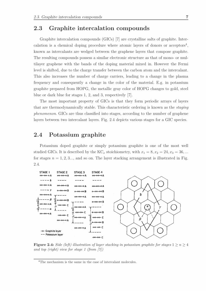
2.4 Potassium graphite

Potassium doped graphite or simply potassium graphite is one of the most well

studied GICs. It is described by the KCx stoichiometry, with x1 = 8, x2 = 24, x3 = 36, ...

for stages n = 1, 2, 3..., and so on. The layer stacking arrangement is illustrated in Fig.

2.4.

Figure 2.4: Side (left) illustration of layer stacking in potassium graphite for stages 1 ≥ n ≥ 4and top (right) view for stage 1 (from [7])

4The mechanism is the same in the case of intercalant molecules.

2.4. Potassium graphite 8

The period of potassium layers can be written as:

Ic = ds + (n − 1)c0, (2.5)

where n is the stage index, c0 = 3.35 Å is the separation of graphene layers, and ds = 5.35

Å is the separation of boundary graphene layers.

In the following, I narrow my scope to the stage 1 compound (KC8) on which my

research was focused on. In this compound, graphene layers are stacked in the AA order

with the position of the potassium atoms varying from layer to layer (see Top view in Fig.

2.4). Its conductivity is highly anisotropic with σab

σc= 56. This material was intensively

studied after it was shown to be superconductor at sub-Kelvin temperatures [21] which

is not observable in neither graphite nor potassium. However this interest has gradually

diminished by the end of the 1980’s.

Nowadays, its study is motivated by the enormous interest in graphene, which re-

quires earlier works to be revisited with emphasis on present expectations. Recent studies

have shown that it is a model system of biased graphene [8] and that both graphene-

derived electrons and graphene-derived phonons are crucial for its superconductivity

[22].

Chapter 3

Theory of electron spin resonance

Electron spin resonance (ESR)1 has become a widespread contact free characteriza-

tion method since its discovery in the 1940’s [23], used in various branches of science

from medicine through chemistry to physics. In physics, it is mainly utilized to examine

the magnetic interactions or spin-dynamics of unpaired electrons, for which it was used

in my research.

In the present chapter, I discuss the theoretical background of this method from

the fundamentals to the specifics regarding conductive samples. In order to properly

deal with the specifics of conduction electron spin resonance (CESR), we first need to

understand the fundamentals of magnetic resonance.

3.1 Basics of magnetic resonance

Magnetic resonance refers to the phenomenon of a resonant transition which arises

in the presence of a magnetic field. It is based on the Zeeman effect, the splitting of

degenerate energy levels when an external magnetic field is applied, which is discussed

in Section 3.1.1. As for a classical oscillator, the amplitude of the transition is only sig-

nificant when the frequency of the excitation matches or is close to that of the resonance.

The width of the resonance is governed by the relaxation rate of the excited electrons,

which is analogous to the damping of a classical oscillator. The resonance dynamics can

be accurately described by empirical equations of motion as it is shown in Section 3.1.2.

3.1.1 The Zeeman effect

Classical electrodynamics states that the magnetic and angular moment of a charged

particle are proportional. The same relation holds true for the equivalent quantum me-

chanical operators:

m = γ~L, (3.1)

1Sometimes referred to as electron paramagnetic resonance

3.1. Basics of magnetic resonance 10

where the proportionality is governed by the γ = q2m

gyromagnetic ratio. Consequently,

the quantized nature of L is conserved in the eigenvalues of m. Here, dimensionless L = L

~

angular momentum operators are used, keeping with the notation of magnetic resonance

literature [24]. For a particle of elementary charge, the µB = e~2me

= 9.274(0) · 10−24 JT

coefficient is the quantum value of the magnetic moment, the Bohr-magneton:

mz = µBlz, (3.2)

The Stern-Gerlach experiment [25] revealed that the electron also possesses an intrin-

sic quantum number which is coupled to its magnetic moment. As it could be interpreted

as the angular moment stemming from an electron spinning around its own axis, the

new quantum number was named. However this classical treatment proved inadequate,

the origin of the spin was explained by the Dirac equation [26], which became the cor-

nerstone of relativistic quantum mechanics. It showed that for spins, the analog of eq.

(3.1) has to be amended by a coefficient of ge = 2, known as the g-factor:

m = γeS = −geµBS (3.3)

Here, S is the dimensionless spin operator and the free electron gyromagnetic ratio (γe)

is defined as

γe = ge

q

2me

= ge

−e

2me

= −geµB, (3.4)

where ge is the free electron g-factor, me is the electron mass, and e is the elementary

charge. The value of the electron g-factor was later refined by quantum electrodynamics,

giving ge = 2.00231(9). Thus the γe

2π≈ 28GHz

Tis obtained.

The energy levels of a system possess a two-fold spin degeneracy in the absence of

a magnetic field energy. This degeneracy is lifted upon the application of a non-zero

magnetic field, as it designates two inequivalent orientations of the spin with different

energies. This is known as the Zeeman effect.

Figure 3.1: Zeeman splitting of an electron (S = 12) induced by an external magnetic field.

It can be formulated by introducing the magnetic energy of the m magnetic moment

associated with the S spin in the Hamiltonian of the system:

HZeeman = −mB = geµBBS = geµBBzsz. (3.5)

3.1. Basics of magnetic resonance 11

The result is a lower energy parallel (mB > 0) and a higher energy antiparallel

(mB < 0) configuration, as shown in Fig. 3.1. By substituting the sz = ±12

eigenvalues

for the two spin orientations of half-spin electrons we get:

∆E = ~ω = geµBBz, (3.6)

the level splitting and transition frequency of this two-level system.

3.1.2 The Bloch equations

The phenomenological description of magnetic resonance was introduced by Felix

Bloch [27] in 1944 by formulating the macroscopic behavior of the M magnetization by

the means of classical electrodynamics. The equations describe the ωL = γeB0 angular

frequency Larmor precession of M around a z-axis magnetic field with M asymptotically

converging into the equilibrium position of M0 ‖ z on a time scale characteristic of the

exponential z-axis relaxation.

dMz(t)dt

= γe[M × B]z +M0 − Mz(t)

T1

(3.7)

Analogously the x, y components will vanish (Mx,y = 0) on a timescale representing the

in-plane loss of the magnetization.

dMx(t)dt

= γe[M × B]x − Mx(t)T2

(3.8)

dMy(t)dt

= γe[M × B]y − My(t)T2

(3.9)

Equations (3.7), (3.8), and (3.9) are the so-called Bloch equations. Generally, the T1

(spin-lattice or longitudinal) and T2 (spin decoherence or transversal) relaxation times

are not equal. However in metals they are equal (T1 = T2) [4].

By solving these equations for a B field composed of a B0 static external field and

small B1(ω) alternating excitation field [24], the magnetization is obtained. The steady

state solution for the x and y magnetization is given in a reference frame rotating at ω.

M ′x =

1µ0

χ0ω0T2(ω0 − ω)T2

1 + (ω0 − ω)2T 22

B1 (3.10)

M ′y =

1µ0

χ0ω0T21

1 + (ω0 − ω)2T 22

B1 (3.11)

Here, the rotating frame is denoted as ′, ω0 = γeB0 is the transition frequency, and the

equilibrium magnetization is formulated as M0 = χ0B0

µ0, as a function of the χ0 static

spin susceptibility.

3.1. Basics of magnetic resonance 12

The solution in the standing reference frame of the laboratory is

Mx(t) = M ′x cos(ωt) + M ′

y sin(ωt) = (χ′ cos(ωt) + χ′′ sin(ωt))Bx0= χBx(t), (3.12)

where the time dependent response is simplified by the introduction of a complex χ

susceptibility:

χ = χ′ − iχ′′, (3.13)

The transition is caused by a circularly polarized field [24, 27], which is only one

component of the applied Bx linearly polarized field, hence Bx0= 2B1. Thus, the real

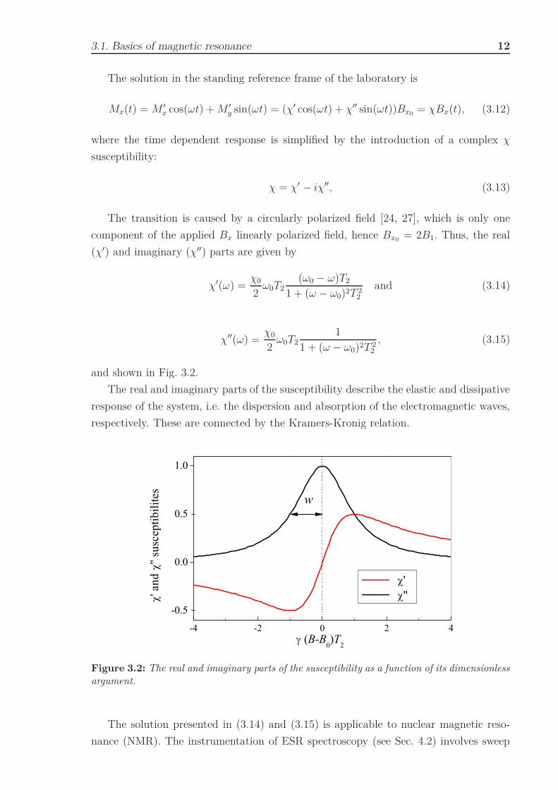
(χ′) and imaginary (χ′′) parts are given by

χ′(ω) =χ0

2ω0T2

(ω0 − ω)T2

1 + (ω − ω0)2T 22

and (3.14)

χ′′(ω) =χ0

2ω0T2

11 + (ω − ω0)2T 2

2

, (3.15)

and shown in Fig. 3.2.

The real and imaginary parts of the susceptibility describe the elastic and dissipative

response of the system, i.e. the dispersion and absorption of the electromagnetic waves,

respectively. These are connected by the Kramers-Kronig relation.

-4 -2 0 2 4

-0.5

0.0

0.5

1.0

' and

'' s

usce

ptib

ilite

s

(B-B0)T

2

' ''

w

Figure 3.2: The real and imaginary parts of the susceptibility as a function of its dimensionlessargument.

The solution presented in (3.14) and (3.15) is applicable to nuclear magnetic reso-

nance (NMR). The instrumentation of ESR spectroscopy (see Sec. 4.2) involves sweep

3.2. Spin susceptibilities 13

of the magnetic field, while keeping the excitation frequency constant and it employs a

detection scheme that measures the derivative of the absorption. Therefore resonances

manifest as derivative Lorentzian curves as a function of the external field:

f(B) = I · dL(B)dB

= I1π

−2w

(w2 + (B − B0)2)2 , (3.16)

where I is the intensity of the normalized L(x)(

∞∫-∞

L(x)dx = 1)

Lorentzian function

with w line-width.

The parameters of the resonance curve can be obtained by comparing (3.15) and

(3.16). The static spin susceptibility appears in the I intensity parameter, the second

integral of the curve2:

I =π

2B0χ0 (3.17)

The w line-width is inversely proportional to the T2 xy-plane spin dephasing time:

w =1

γT2(3.18)

The third important parameter of the curve is the resonance field, from which the

g-factor can be calculated. The magnetic field acting on unpaired electron of the sample

is a local Bloc field, the B0 external field supplemented by the field of the electrons and

nuclei of the sample. This is detected as an apparent resonance field, different from what

we would expect for free electrons, and treated as a g = geξ departure from ge = 2.0023:

~ω = ∆E = geµBBloc = geµB(B0ξ) = (geξ)µBB0 = gµBB0 (3.19)

3.2 Spin susceptibilities

The ESR signal is proportional to the susceptibility of the measured sample. This

section summarizes the relevant static spin susceptibilities [28] in the materials studied

herein.

Materials composed of non-interacting unpaired electrons will act as an ensemble of

independent magnetic moments. The magnetization of such materials can be formulated

by the means of statistical physics. This yields a magnetization of:

〈M〉 =N

VgJµBJBJ

(gJµBB0J

kBT

)(3.20)

where gJ is the Landé g-factor, J is the total angular momentum quantum number, and

BJ(x) is the so-called Brillouin-function:

2This is the area under the Lorentzian curve of the resonance

3.3. Conduction electron spin resonance 14

BJ(x) =2J + 1

2Jcoth

(2J + 12J

x)

− 12J

coth( 1

2Jx)

(3.21)

We operate far from the saturation of the magnetization, so we shall consider the

case of B0 → 0 external field. We arrive at the expression of

χCurie0 = µ0 lim

B0→0

M0

B0= µ0

S(S + 1)g2µ2B

3kBT

1VC

, (3.22)

which is known as the Curie susceptibility. Eq. (3.22) is inversely proportional to the

VC = VN

unit cell volume, and the temperature, T . Note that J has been replaced

by S as the L orbital momentum will be quenched [24] for studied materials of Curie

susceptibility.

Our research was focused on conductive samples. The paramagnetism of the unbound

electrons is qualitatively different from that of the localized spins. Electrons obey the

Fermi-Dirac distribution:

f(ε) =1

eβ(ε−µc) + 1. (3.23)

When a magnetic field is applied, the Fermi level of the spin-up and spin-down con-

figurations will be shifted by equal values but in the opposite direction. It results in a

small surplus of one spin species. This paramagnetic moment is generated by the elec-

trons close to the Fermi energy, thus the susceptibility will be proportional to the Fermi

energy density of states:

χPauli0 =

14

g2eµ0µ

2Bg(EF)

1VC

(3.24)

where g(EF) is the atomic density of states at the Fermi energy. Eq. (3.24) is referred

to as the Pauli susceptibility and is usually two orders of magnitude smaller than the

Curie susceptibility.

3.3 Conduction electron spin resonance

The experimental and theoretical investigation of electron spin resonance in metals

was pioneered in the early half of the 1950’s by the group of Arthur Kip and Charles

Kittel [29] at Berkeley with theorists working alongside them such as Freeman Dyson

and Yako Yafet. After preliminary calculations for the g-factor shift of sodium [30], the

group successfully observed the spin resonance of the conduction in metallic sodium [31].

This result was only the forerunner of later results wchich provided theories explaining

the underlying physics. Dyson explained the anomalous absorption curve [32, 33], while

Elliott’s consideration of the spin orbit shed light on the spin relaxation mechanism of

metals and semiconductors [34], the results of both will be reviewed in Sections 3.3.2 and

3.4, respectively. These treatises paved the way for spin resonance studies in conductive

samples, broadly termed as conduction electron spin resonance (CESR).

3.3. Conduction electron spin resonance 15

3.3.1 The skin effect

In order to understand the response of conduction electrons, the penetration of mi-

crowaves in a conductive sample has to be considered.

According to Ohm’s law the free current density is proportional to the electric field:

jf = σE (3.25)

with a coefficient of σ, the conductivity.

To look for a steady state solution without any accumulated surface charge density,

we fix ρf = 0. This is in accordance with ∇jf = −∂ρf

∂t, the continuity equation of the

free charge density.

With these conditions, Maxwell’s equations take the following form:

∇ · E = 0 (3.26)

∇ · B = 0 (3.27)

∇ × E = −∂B

∂t(3.28)

∇ × B = µE + µε∂E

∂t(3.29)

Applying curl to (3.28) and (3.29), we arrive at a modified wave equation for the

conductive medium:

∇2B = µ0ǫ0∂2B

∂t2+ µσ

∂B

∂t. (3.30)

We shall solve this with a plane wave ansatz of

B(z, t) = B0ei(kz−ωt) (3.31)

which yields an unmodified ω and a complex wave vector of

k =√

µεω2 + iµσω = k + iκ, (3.32)

which can be written as the sum of a real (k) and an imaginary part (κ), which are

defined as

k =2π

λ=ω

√εµ

2

√

1 +(

σ

ωε

)2

+ 1

12

, and (3.33)

κ =1δ

=ω

√εµ

2

√

1 +(

σ

ωε

)2

− 1

12

. (3.34)

The result is an attenuated wave,

B(z, t) = B0e− z

δ ei(kz−ωt), (3.35)

3.3. Conduction electron spin resonance 16

with its amplitude decreasing exponentially as a function of z. The δ length scale of the

attenuation—defined in (3.34)—is known as the skin depth.

This behavior is depicted in Fig. 3.3. For a highly conductive medium, the wavelength

of the incident microwave is several orders of magnitude greater than in the medium,

where λ ≈ 2πδ.

-3 -2 -1 0 1 2 3 4 5

0

1 MetalB||(0)

B||(z)

e-z/

z/

Vacuum

Figure 3.3: Illustration of the skin effect. The magnitude of the alternating magnetic fielddecreases exponentially on a length scale of δ. Note the severe decrease in wavelength for theconductive medium.

The complex wave vector will also result in a φ phase difference for the penetrating

electric and magnetic fields.

φ = tan−1 κ

k(3.36)

3.3.2 The Dysonian line shape

The previous section showed that for conductive samples, the alternating microwave

field will penetrate only skin depth. This leads to an anomalous absorption derivative

ESR signal [32]. The line shape of conductive samples was formulated by Dyson [33],

hence they are referred to as Dysonian lines.

Dyson considered that although electrons are only excited within the penetration

depth, their diffusion is not limited to it. Electrons can diffuse in and out of the skin

depth, resulting in a rather complex response of the material. Correspondingly, the line

shape will be described as a function of the usual parameters of the g-factor, the static

spin susceptibility (χ), spin relaxation time (T2) and the newly included parameters of

R and λ. These parameters are defined as

R =

√TD

T2, (3.37)

the square root of the ratio of the electron diffusion time across the skin depth (TD) and

3.3. Conduction electron spin resonance 17

the spin relaxation time (T2), and

λ =d

δ, (3.38)

the ratio of the sample size (d) and the skin depth (δ).

The detected signal is the frequency derivative3 of the real part of a rather elaborate

complex formula, and can be written as [35]:

dP

dω= N

Re(F 2) Re

[dG(ω − ω0)

dω

]−[Im(F 2) Im

dG(ω − ω0)dω

](3.39)

where F is a function of u, which are defined as

F = −u tan(u) (3.40)

u =λ

2(1 + i). (3.41)

The G(ω − ω0) is defined as4

G(ω − ω0) =i

(w2 − u2)

[2u2 cot(w)

w+ (w2 − 3u2)

cot(u)u

+ (w2 − u2)cosec2(u)

], (3.42)

where

w =λR

2(ξ + iη) (3.43)

is a function of

ξ = [sgn(x)][(1 + x2)12 − 1]

12 , and (3.44)

η =[(1 + x2)12 + 1]

12 , (3.45)

which bear an argument of

x = (ω − ω0)T2. (3.46)

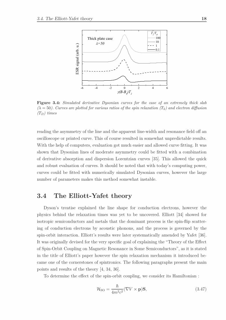
Simulated Dysonian curves are plotted in Fig. 3.4 for different R ratios. Note that

as the the ratio increases, so does the asymmetry of the derivative line, resulting in

an extreme case where the signal resembles a Lorentzian curve instead of a derivative

Lorentzian.

This formula is rather hard to comprehend or even try to give it a simple inter-

pretative picture. Before computer assisted data analysis, such lines were evaluated by

3As for the Bloch equations, the response is formulated as a function of the ω excitation and ω0

resonance frequencies.4This function differs in a factor of i in Refs. [33] and [35], here we adopt the function in Dyson’s

original paper [33].

3.4. The Elliott-Yafet theory 18

-6 -4 -2 0 2 4 6

ESR

sign

al (a

rb. u

.)

(B-B0)T2

T2/TD

100 10 1 0.1

Thick plate case=50

Figure 3.4: Simulated derivative Dysonian curves for the case of an extremely thick slab(λ = 50). Curves are plotted for various ratios of the spin relaxation (T2) and electron diffusion(TD) times

reading the asymmetry of the line and the apparent line-width and resonance field off an

oscilloscope or printed curve. This of course resulted in somewhat unpredictable results.

With the help of computers, evaluation got much easier and allowed curve fitting. It was

shown that Dysonian lines of moderate asymmetry could be fitted with a combination

of derivative absorption and dispersion Lorentzian curves [35]. This allowed the quick

and robust evaluation of curves. It should be noted that with today’s computing power,

curves could be fitted with numerically simulated Dysonian curves, however the large

number of parameters makes this method somewhat instable.

3.4 The Elliott-Yafet theory

Dyson’s treatise explained the line shape for conduction electrons, however the

physics behind the relaxation times was yet to be uncovered. Elliott [34] showed for

isotropic semiconductors and metals that the dominant process is the spin-flip scatter-

ing of conduction electrons by acoustic phonons, and the process is governed by the

spin-orbit interaction. Elliott’s results were later systematically amended by Yafet [36].

It was originally devised for the very specific goal of explaining the “Theory of the Effect

of Spin-Orbit Coupling on Magnetic Resonance in Some Semiconductors”, as it is stated

in the title of Elliott’s paper however the spin relaxation mechanism it introduced be-

came one of the cornerstones of spintronics. The following paragraphs present the main

points and results of the theory [4, 34, 36].

To determine the effect of the spin-orbit coupling, we consider its Hamiltonian :

HSO =~

4m2c2(∇V × p)S, (3.47)

3.4. The Elliott-Yafet theory 19

where m is the free electron mass, V is the scalar potential with no spin dependent

terms, p is the linear momentum operator and S is the spin operator. Bloch states of a

single spin configuration will not be eigenstates of the spin operator. Treating the HSO

term as a perturbation, we attain an admixture of spin-up and spin-down Bloch states

with k lattice momentum.

Ψk,↑(r) = (ak(r) |↑〉 + bk(r) |↓〉) eikr (3.48)

Ψk,↓(r) =(a∗

−k(r) |↓〉 + b∗

−k(r) |↑〉

)eikr (3.49)

where ak and bk lattice-periodic coefficients which reflect the symmetry properties of the

solid, like the uk function of Bloch states. HSO couples electron states of opposite spins,

same k, but different bands. The perturbation treatment yields ak, bk coefficient of:

|a| ≈ 1, and |b| ≈ λ

∆E(3.50)

where λ is the matrix element of the spin-orbit term5 for the conduction and a near-lying

band of the same k, and ∆E is the energy separation of the aforementioned bands. The

admixture ratio is dependent of the spin-orbit interaction strength which scales as Z4

(Z is the atomic number) and the shape of the Fermi surface.

Elliott estimated the g-factor shift to be in the order of magnitude of the admixture.

∆g = g − ge = α1|bk||ak| = α1

λ

∆E, (3.51)

where ge = 2.00231(9) is the free electron g-factor, α1 = 1..10 is a constant over unity,

determined by the band structure.

The spin-orbit alone does not induce spin flipping and spin relaxation, it is only

responsible for inducing the mixed spin-state. The spin-flip scattering stems from the

same interaction Hamiltonian as for momentum scattering with no spin-flip. Impurities

produce a constant, temperature independent term in 1τ, it is responsible for the residual

resistivity. The contribution of phonons is given by the so called Bloch-Grüneisen curve,

which is linear for high temperatures and follows a T 5 dependence well below the Debye

temperature.

Using Fermi’s golden rule for the mixed spin-state Bloch-type wave functions we

defined in (3.48) and (3.49), the momentum relaxation time, characteristic of scattering

is given by1τ

∝∣∣∣∣∫

a∗k′Hintakei(k−k′)rdt

∣∣∣∣2

, (3.52)

while the spin relaxation time, characteristic of spin-flipping is given by

1T1

∝∣∣∣∣∫

(a−k′Hintbk − b−k′Hintak)ei(k−k′)rdt∣∣∣∣2

. (3.53)

5This should not be confused with the spin-orbit constant

3.4. The Elliott-Yafet theory 20

This yields the following relation between the relaxation times:

1T1

= α2|bk||ak| = α2

(λ

∆E

)2 1τ

(3.54)

where α2 is a band structure dependent constant in the order of unity.

Although the proportionality to the resistivity the ESR line-width:

w ∝ 1T1

∝ ρ, because ρ ∝ 1τ

(3.55)

might seem straightforward, it is not trivial for the whole of the temperature dependence.

The connection between the temperature dependence of 1T1

an that of the resistivity was

unambiguously proven by Yafet [36], thus

1T1

(T ) ∝ 〈b〉2 ρ(T ), (3.56)

is known as the Yafet relation.

Figure 3.5: Schematics of the Elliott-Yafet spin relaxation mechanism. Left (A): The evolutionof the electron spin during transport (from [37]). Right (B): The spin scattering process. Thespin-orbit interaction induces an admixture of spin-up and spin-down states, which occasionallyleads to a spin flip (from [38]).

The attained spin relaxation mechanism is illustrated in Fig. 3.5. Inset A illustrates

the propagation of the spin, with spin flips occurring only if momentum scattering oc-

curs. Inset B shows that the SO coupling forms a mixed spin state, which allows the

momentum scattering interaction term to induce spin flipping with a small probability.

This theory [34, 36] explained the CESR for most pure metals [39, 40]. Its validity

was shown in a generalized form for one-dimensional metals [41]. Consideration of the

shape of the Fermi surface in polyvalent metals resulted in the “spin hot spot model”

[42, 43]. A generalized approach explained the CESR behavior of strongly correlated

metals such as MgB2 [44], K3C60, and Rb3C60 [45], where the ~

τscattering rate is in the

order of the ∆E band separation.

Chapter 4

Sample preparation and

experimental setup

This chapter discusses the technical details of graphite intercalation, sample handling,

as well as the experimental setup used for temperature dependent conduction electron

spin resonance spectroscopy.

4.1 Sample preparation

Alkali doped graphite samples were prepared from 3 mm diameter disks of grade I

HOPG (SPI Supplies) and high purity fine powder graphite (Fisher Scientific).

The powder samples, although finely ground, formed larger granules upon doping.

The formation of macroscopic metallic clusters was unfavorable as microwave penetration

was limited to the skin depth as in the HOPG samples. To counter the conglomeration of

the powder samples and allow efficient microwave penetration, the graphite was mixed

together with an equal mass of a dilute (1.5 ppm) mixture of manganese and magnesium-

oxide (Mn:MgO) prior to doping. The ESR-silent and doping insensitive MgO performed

the separation of the graphite crystallites, while Mn2+ had the added benefit of being a

g-factor and susceptibility standard.

Prior to intercalation, the graphite samples were vacuum annealed at 500 C in a

quartz tube. Afterwards samples were handled in an argon filled glove box (Fig. 4.1E) to

avoid exposure to oxygen and water. Alkali metals were heated to temperatures above

their melting point (typically 120C < T < 150C), upon melting they were soaked into

small glass capillaries in which they solidified after cooling. The sample and the capillary

of alkali metal were vacuum sealed quartz doping ampoule (Fig. 4.1A & 4.1B). Doping

was achieved through two-zone vapor transport intercalation [7], which is explained in

the following. Abundant amounts of alkali were used to ensure saturation doping. The

resulting compounds (e.g. Fig. 4.1C & 4.1D) were transferred from the doping vessel to

a clean quartz tube in the inert atmosphere of the glove box and sealed under helium

for the measurements with a pressure of 20 mbar. As described in Section 2.3, doping

4.1. Sample preparation 22

modifies color of the HOPG samples, attesting its success. In the case of stage 1 and

stage 2 potassium graphite, to gold (Fig. 4.1C) and blue (Fig. 4.1D), respectively. In

some cases for the stage 1 species, the brief exposure to Ar induces a slight surface

dedoping, which is seen from the change in the color of the samples from gold to red,

however this does not modify our results significantly, as the bulk of the material remains

unchanged.

Figure 4.1: Key elements of sample preparation: illustration (A) and photograph (B) of quartzsample holder for doping, which is narrowed to separate the two materials; synthesized stage 1KC8 (C) and 2 KC24 (D) potassium doped HOPG compunds after transfer, with distinctive goldand metallic blue colors; MBRAUN Unilab inert gas glove box (E) operated with Ar atmosphere.

The two-zone vapor method requires the temperature of the graphite host and the

intercalant to be independently adjusted, this relies on the spatial separation of the two

materials. The intercalant is heated to higher Ti temperatures thus allowing the alkaline

vapor to condense in the somewhat colder (Tg) graphite and form a crystalline salt. By

increasing the temperature gradient between the sample and the dopant, higher stages

become thermodynamically more stable thus the staging phenomenon can be controlled.

The temperature gradients for alkali metals are well documented in Ref. [7] and served

as the basis of our synthesis as well. Their typical values for the studied K, Rb and Cs

intercalants are given in Table 4.1.

Table 4.1: Temperature gradients for alkaline two-zone vapor doping (stages 1 < n < 3)

K Rb CsTi = 250 C Ti = 208 C Ti = 194 C

Stage Tg(C)

1 225-320 215-330 200-4252 350-400 375-430 475-5303 450-480 450-480 550

4.2. ESR spectrometer setup 23

Figure 4.2: Schematic diagram of the implemented two-zone intercalation setup and its tem-perature profile, illustrated in the top plot.

Fig. 4.2. shows the two-zone doping setup assembled as part of the thesis project and

used for sample synthesis. In our setup, the separation of the two materials was achieved

with the use of inexpensive, home-made doping ampoules: long quartz diameter tubes(ø4

mm) with a middle section narrowed with the use of an oxyacetylene blow torch. The

setup is based on the local heating of the alkali intercalant. A ø10 mm quartz tube is

placed in a tube furnace which sets the Tg temperature. The surplus heating, needed for a

higher Ti is achieved with a Joule heating coil, powered by a controllable voltage source.

The resistive heater wire is wrapped around a narrowed section of the tube which ensures

the proper placement of the sample. The coil is surrounded by an insulating ceramic tube

to prevent significant radiative heat loss. The Ti and Tg temperatures at the two ends

of the ampoule are measured with two thermocouples. Thermal insulation fabric was

added to the openings of the furnace ensuring thermal stability.

4.2 ESR spectrometer setup

In this section, I present the operating principles of a standard X-band ESR spec-

trometer, which was the instruments of choice for my research. Afterwards the specifics

of the measurements will be discussed. The schematics of the high field ESR is discussed,

where some of the experiments were performed.

4.2.1 X-band ESR

Experiments at 9 GHz were carried out using two X-band ESR spectrometers. Tem-

perature dependent measurements in the 100-600 K range were performed on a modified

JEOL spectrometer optimized for highly conductive samples, while the low temperature

range of 4-250 K was covered with a commercial Bruker Elexsys E500 in the laboratory

of Prof. László Forró at the EPFL.

4.2. ESR spectrometer setup 24

Figure 4.3: Schematic diagram of the ESR spectrometer

Figure 4.3. depicts the layout of an X-band ESR spectrometer. This reflection ge-

ometry measures the power reflected from the microwave cavity containing the sample,

indirectly gathering information from the absorption process.

First, the elements of the microwave bridge are discussed. A tunable frequency mi-

crowave source provides the electromagnetic excitation. Its output is split into 3 paths,

one connected to the cavity, a second as a reference arm for the detector and a minis-

cule portion of the waves is coupled into a microwave frequency counter. The first arm

is connected to a microwave cavity via waveguides. The power of the incident waves

can be adjusted using a tunable attenuator. Microwaves going to and coming form the

cavity are separated with a circulator, a non-reciprocal three-port terminal in which the

reflected wave is transmitted to a different port than the incident wave, thus directing

only the reflected radiation to the detector.

Figure 4.4: Details of the cavity: Cavity geometry [46] (A), cavity resonance [47] (B), iris forcavity impedance adjustment [47] (C).

The cylindrical cavity determines a TE011 standing wave mode for the alternating

field inside. As it is shown in Fig. 4.4A, this arrangement gives a linearly polarized

magnetic field for excitation and also separates the electric and magnetic components in

4.2. ESR spectrometer setup 25

space. The cavity resonator acts as an amplifier for the phenomenon we wish to observe,

for maximum effect the frequency of the excitation has to match that of the resonance1.

At resonance, the power absorbed by the cavity and the alternating field inside are maxi-

mal (Fig. 4.4B). As slight variation of this condition ruins the experiment, it is critical to

remain in resonance. This is achieved with a automatic frequency control (AFC) circuit

in the microwave bridge. The efficiency of this negative feedback is determined by the

quality factor of the resonator, which has the following two equivalent definitions:

Q = 2πEenergy stored

Eenergy dissipated in one period=

ω0

∆ω(4.1)

The amount of photons reflected from and entering the cavity can be adjusted with

the so-called iris element of the cavity which tunes the impedance of the waveguide and

resonator. For optimal operation there is no reflection at resonance, this is the so-called

critical coupling [48].

The microwave of the reference arm is additively mixed with the microwave reflected

from the cavity by a magic tee coupler. The phase of the reference arm is adjusted to

reach maximum constructive interference. The reference signal does not affect the signal

of the cavity, it only adds a constant (DC) term to the incident power on the detector.

This acts as a bias to set the semiconductor diode detector to its operating point to

ensure optimal sensitivity.

A water-cooled external electromagnet is used to induce Zeeman splitting. As shown

previously, electron spin resonance occurs when the energy of the excitation photons

matches that of the induced level splitting. This causes a resonant absorption of the

microwave which is accompanied by a slight increase in the signal reflected from the

cavity. Contrary to optical or transport measurements, electron spin resonance is probed

by varying the B0 external field and keeping the excitation frequency stable. This stems

from the technical difficulty of producing stable broadband microwave equipment.

The identification of the minuscule ESR signal from the noisy detector signal requires

a technique called phase sensitive or lock-in detection. This scheme allows the weak

response of a probed phenomenon to be distinguished from the noisy environment by

modulating a weak signal at a high frequency and detecting at the same frequency. In

ESR spectrometers the linear sweep external B0 magnetic field is modulated by the

built-in “modulation coils” of the cavity. It operates with the amplified AC reference

signal of the lock-in detector and produces a Bmod(fmod) ‖ B0 field and alternates at

high frequencies.

The effect of the modulation can be calculated from the detector output induced by

the response of the cavity at resonance. The power emitted by the cavity at resonant

absorption is given by the following formula [24]:

1The cavity resonance should not be mistaken for the resonant absorption due to the electron spinflip.

4.2. ESR spectrometer setup 26

P =1

πµ0|B1|2 ωχ′′(ω)V (4.2)

where µ0 is the vacuum permeability, B1 is the alternating excitation field of the cavity.

The detector voltage difference at resonant absorption is proportional to the macro-

scopic magnetic moment of the studied sample [46, 48]:

∆Udet ∝ m ∝ χ′′V B1 (4.3)

By taking the series expansion of χ′′ and neglecting higher order terms, the lock-in

scheme averages out the constant term and preserve the first derivative of the suscepti-

bility:

χ′′ ≈ χ′′B0

+dχ′′

dB B0

∆B. (4.4)

As a result, the output of the lock-in amplifier will be proportonal to the following

quantities:

ULock-in ∝ dχ′′

dB0V B1Bmod ∝ dχ′′

dB0V√

PMWBmod, (4.5)

where PMW ∝ |B1|2 was taken into account.

As the magnitude of the processed signal is proportional to dχ′′

dB0, resonances arise as

derivative Lorentzian curves in the ESR spectra (as depicted in Fig. 4.5.).

-4 -2 0 2 4

0.0

0.5

1.0

-4 -2 0 2 4

-0.5

0.0

0.5

(B0-Bres

0)T

2

w

B0+B

modcos(

modt)

Lore

ntzi

an c

urve

(B

0-Bres

0)T

2

Derivative Lorentzian curve

Figure 4.5: Effect of the lock-in method on the Lorentzian lineshape.

As opposed to commercial solutions (e.g. Bruker), the modified JEOL setup has a few

unique properties, which are highlighted here. The determination of the magnetic field

was originally calculated from the current of the electromagnet. To ensure precise scale

calibration, a Hall effect sensor was added. The JEOL spectrometer setup was optimized

4.2. ESR spectrometer setup 27

for experiments on high loss, metallic samples, by utilizing a low Q cavity (Q ≈ 1000).

The extreme high conductance of some samples significantly lowered the quality factor

of the cavity and in several instances, critical coupling could not be achieved. The same

was true for low conductance samples, as critical coupling was out of the range of iris

operation.

In the case of both spectrometers, communication with the instruments and data

acquisition is handled by computer software.

Both setups can accommodate temperature dependent experiments. The Bruker sys-

tem is operated with a commercial liquid helium cryostat, covering the 3.5-250 K range.

The temperature is adjusted with built in PID controlled heater. Temperature control

in the JEOL system io realized with a home-made nitrogen gas circulation system. Op-

eration is possible up to ∼ 700 K and down to a few degrees above the boiling point of

liquid nitrogen (77 K).

4.2.2 High frequency ESR

High field measurements were performed on a home built quasi-optical continuous

wave ESR spectrometer [49] at 111 GHz (∼ 4 T resonance field) in the laboratory of

Prof. András Jánossy.

Figure 4.6: Schematics of the high frequency ESR setup. The microwave radiation is emittedfrom the (1) microwave source, passes through the (2) isolator (45 Faraday rotator), (3) beamsplitter, (4) phase shifter, (5) attenuator and enters the (7) probe head through the (6) gridfor “polarization coding”. The reference signal is directed towards the (8) 90 Faraday rotator,and then joins the signal with orthogonal polarization at grid (9). Finally the signal and thereference, added at the (10) rotating grid, enter the (12) detector isolated from the bridge bythe (11) 45 Faraday rotator (from [49])

4.2. ESR spectrometer setup 28

Waveguides and cavity resonators are not applicable for microwaves of such small

wavelengths, hence the microwave bridge is replaced by an elaborate system of quasi-

optical elements (Fig. 4.6) and more sensitive detectors. The resonance field associated

with these higher frequencies requires the use of superconducting magnets. The higher

resonance field significantly increases the resolution of the measurements, however this

advantage also inhibits most CESR experiments. The skin effect is significantly magni-

fied, penetration depth is 3.5 times smaller for 111 GHz than for the 9 GHz studies. The

liquid helium cryostat limited the studied temperature range to below 270 K.

Chapter 5

Results and discussion

The present chapter exhibits the results of my studies, their evaluation and the

conclusions. I focus on stage 1 potassium graphite (KC8), synthesized with different

starting graphite materials. The results are discussed in the theoretical framework of

electron spin relaxation.

5.1 The CESR signal of doped graphite

The first step in the investigation of CESR in potassium graphite was a preliminary

study of the effect of doping in graphite. The effect of the doping time was studied

on a graphite powder sample mixed with Mn:MgO. Intercalation was done at 300C in

intervals with an extremely narrowed doping ampoule, to allow sufficient control over

the intercalation process. The CESR spectrum was acquired after each step.

310 320 330 340 350 360

Bab0

ESR

sig

nal (

arb.

u.)

Magnetic field (mT)

Bc0

Figure 5.1: CESR spectrum of pristine graphite powder mixed with Mn:MgO (black curve)and the corresponding powder average fit (red curve), and the powder average simulated fornarrower lines (blue curve). The sextet line arises from the hyperfine splitting of the Mn2+

ions.

5.1. The CESR signal of doped graphite 30

The 2 + 1 dimensional structure of pristine graphite is reflected in its electronic

properties. The g-factor and line-width are anisotropic, especially at low temperatures

[50, 51]. For a powder sample, the anisotropy is expected to produce a curious shape as

the measured signal is a powder average of the g-factor and line-width over the possible

orientations of the graphite microcrystallites. As Fig. 5.1 shows, the measured spectra

and the simulated powder average fits are in a good agreement.

330 335 340 345 350 0 5 10 150

20

40

60Doping time (in hours)

0.5 1 1.5 2 2.5 4 5 10

ESR

sign

al(a

rb. u

.)

Magnetic field (mT)

Norm

. ESR intensity(arb.u.)

Doping time (h)

Figure 5.2: Doping time dependence of the CESR spectrum (left) and CESR intensity (right).

The doping time dependence of the ESR spectra is presented in Fig. 5.2. A symmetric

line emerges beside the anisotropic signal of pristine graphite for low doping. As the

doping time increases, the line dominates over the other signal. The onset of the doping

is slow, however once it occurs, the signal intensity steadily increases without a significant

change in the line-width. The unchanged line-width indicates stable conditions and the

formation of the same stage configuration for short and long doping times. The signal

intensity did not change after 25 hours of doping which indicated the saturation of the

doping. For normal doping vessels this time was considerably shorter.

The doping dependence of the ESR signals was followed by the investigation of sat-

uration doped compounds from both HOPG and graphite powder hosts prepared as

described in Sec. 4.1. The X-band spectra of the stage I potassium doped graphite com-

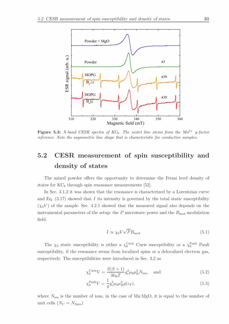
pounds are shown in Fig. 5.3. Dysonian line shapes [32, 33] are observed, characteristic of

conducting samples, where only the surface conduction electrons within the skin depth

are affected by the microwave excitation. As we move from the HOPG slab to the well

dispersed powder the asymmetry is less profound and is accompanied by stronger signals.

This is due to the decrease in the ratio of the grain size and skin depth, which results

in a better microwave penetration for separated crystallites. In all cases, asymmetry is

moderate enough to fit the spectra with a combination of absorption and dispersion

Lorentzian lines [35]. Intensity, resonance field, and line-width are acquired from these.

5.2. CESR measurement of spin susceptibility and density of states 31

310 320 330 340 350 360

B0 c

B0||cHOPG

Magnetic field (mT)

x30

Powder + MgO

ESR

sign

al (a

rb. u

.)Powder

HOPG x30

x3

Figure 5.3: X-band CESR spectra of KC8. The sextet line stems from the Mn2+ g-factorreference. Note the asymmetric line shape that is characteristic for conductive samples.

5.2 CESR measurement of spin susceptibility and

density of states

The mixed powder offers the opportunity to determine the Fermi level density of

states for KC8 through spin resonance measurements [52].

In Sec. 3.1.2 it was shown that the resonance is characterized by a Lorentzian curve

and Eq. (3.17) showed that I its intensity is governed by the total static susceptibility

(χ0V ) of the sample. Sec. 4.2.1 showed that the measured signal also depends on the

instrumental parameters of the setup: the P microwave power and the Bmod modulation

field.

I ∝ χ0V√

PBmod (5.1)

The χ0 static susceptibility is either a χCurie0 Curie susceptibility or a χPauli

0 Pauli

susceptibility, if the resonance stems from localized spins or a delocalized electron gas,

respectively. The susceptibilities were introduced in Sec. 3.2 as

χCurie0 V =

S(S + 1)3kBT

g2eµ0µ

2BNion, and (5.2)

χPauli0 V =

14

g2eµ0µ2

Bg(εF), (5.3)

where Nion is the number of ions, in the case of Mn:MgO, it is equal to the number of

unit cells (NC = NSpin)

5.2. CESR measurement of spin susceptibility and density of states 32

For Mn2+ ions, a spin of SMn2+ = 52

yields S(S + 1)Mn2+ = 354

, however only the∣∣∣−12

⟩⇔∣∣∣1

2

⟩transitions of these ions are detectable in ESR. This means that S(S + 1) is

replaced by an effective value of 〈S(S + 1)〉Mn2+ = 94, which is derived from the matrix

element of mentioned spin flip transition.

The cMn2+ = 1.5 ppm concentration of Mn2+ ions in MgO was determined through

signal intensity comparison with a known amount of CuSO4 · 5H2O with SCu2+ = 12

and

S(S + 1)Cu2+ = 34. Thus we acquire the molar susceptibility of the Mn:MgO mixture (in

CGS units): χCurie0,mol(Mn:MgO) = 5.641 · 10−9 emu

mol.

With this susceptibility reference, the ratio of the intensities yields the susceptibility

of the sample:

ISample

IMn:MgO

=χ0,mol(Sample)

χ0,mol(Mn:MgO)nSample

nMn:MgO

(5.4)

χ0,mol(Sample) = χ0,mol(Mn:MgO)ISample

IMn:MgO

nMn:MgO

nSample

(5.5)

Similarly, the density of states of a Pauli susceptibility sample is given by the ratio

of intensities with a reference

IPauli

ICurie=

1S(S + 1)

34

kBTg(εF)NPauli

NCurie(5.6)

g(εF) =IPauli

ICurieS(S + 1)

43

Nion1

kBT(5.7)

where g(EF) is the density of states at the Fermi level, measured in units stateseV·C atom

.

These susceptibility measurements require high reproducibility, this demands the use

of the same instrumental parameters and place the sample in the same position every

time. Through mixing with an equal mass of Mn:MgO two problems due to the skin effect

were circumvented. Firstly, the separation of the graphite crystals increased microwave

penetration and thus the S/N ratio. Secondly, the reduction of the studied volume does

not impede the calculation of the density of states as only the relative intensities are

required for the homogeneous powder. A modulation field of Bmod = 10−4 mT enhance

the signal, but did not lead to a distorted resonance line. Microwave power was set to

P = 10 mW as Mn2+ lines were not distinguishable at lower powers. This is undesirable

as it leads to microwave saturation for the manganese. Thus such measurements, where

the reference manganese signal is reduced due to saturation, produce lower intensities

than expected and seemingly increase the susceptibility and density of states values.

Despite this, it is still applicable with an error well within an order of magnitude.

Table 5.1 gathers density of states and spin susceptibility measurements. The data

are in agreement with values from literature [53–55].

5.3. Testing the Elliott-Yafet mechanism in KC8 33

Table 5.1: Density of states and spin susceptibilities in KC8.

χ0 g(EF)(10−6 emu/g) (states/eV·C atom)

CESR 0.92(3)-0.95(6) 0.33(5)-0.34(7)specific heat [53, 54] - 0.327,0.35susceptibility measurement [55] 0.62 -

5.3 Testing the Elliott-Yafet mechanism in KC8

The validity of Elliott-Yafet theory is tested in KC8 measurement of the shift in the

g-factor and comparison of the temperature dependence of the line-width with resistivity

data from literature.

CESR spectra of both HOPG and powder morphologies were acquired for the tem-

perature range of 4-500 K with a typical microwave power of 10 mW and modulation of

0.1-0.2 mT. The high conductance of the samples significantly lowered the quality fac-

tor of the cavity and in several instances critical cavity coupling could not be achieved.

HOPG samples are measured for both c-axis and in-plane (ab) B0 external fields, the

orientation of the fields and the sample are shown in Fig. 5.4.

Figure 5.4: Orientation of B0 and B1 with regard to the disk shaped HOPG sample.

Fig. 5.5. shows the temperature dependence of the ESR line-width—proportional to

the inverse spin relaxation time (∆B = 1γT2

)—for different compounds. Doped HOPG

samples were only studied up to 450 K, above this temperature the potassium on the

surface of the graphite slab begins to evaporate and simultaneously diffuse into the inside

of the disk, effectively dedoping the sample surface (which is otherwise sensed by ESR).

The helium cryostat of the high field spectrometer limits the studied temperature range

of such measurements to below 270 K.

The HOPG and powder samples show the same trends in line-width temperature

dependence for both frequencies. The curves differ mainly in a constant line-width term

and only slightly in the line-width term from homogeneous broadening. The data for

the HOPG sample are in agreement with data obtained by Lauginie et al. in [56] with

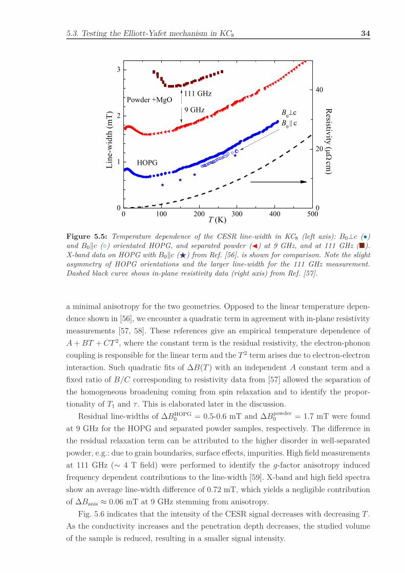
5.3. Testing the Elliott-Yafet mechanism in KC8 34

0 100 200 300 400 5000

1

2

3

B0

cB

0c9 GHz

111 GHz

HOPGLine

-wid

th (m

T)

T (K)

Powder +MgO

0

20

40

Resistivity (

cm)

Figure 5.5: Temperature dependence of the CESR line-width in KC8 (left axis): B0⊥c (•)and B0‖c () orientated HOPG, and separated powder () at 9 GHz, and at 111 GHz ().X-band data on HOPG with B0‖c (⋆) from Ref. [56]. is shown for comparison. Note the slightasymmetry of HOPG orientations and the larger line-width for the 111 GHz measurement.Dashed black curve shows in-plane resistivity data (right axis) from Ref. [57].

a minimal anisotropy for the two geometries. Opposed to the linear temperature depen-

dence shown in [56], we encounter a quadratic term in agreement with in-plane resistivity

measurements [57, 58]. These references give an empirical temperature dependence of

A + BT + CT 2, where the constant term is the residual resistivity, the electron-phonon

coupling is responsible for the linear term and the T 2 term arises due to electron-electron

interaction. Such quadratic fits of ∆B(T ) with an independent A constant term and a

fixed ratio of B/C corresponding to resistivity data from [57] allowed the separation of

the homogeneous broadening coming from spin relaxation and to identify the propor-

tionality of T1 and τ . This is elaborated later in the discussion.

Residual line-widths of ∆BHOPG0 = 0.5-0.6 mT and ∆Bpowder

0 = 1.7 mT were found

at 9 GHz for the HOPG and separated powder samples, respectively. The difference in

the residual relaxation term can be attributed to the higher disorder in well-separated

powder, e.g.: due to grain boundaries, surface effects, impurities. High field measurements

at 111 GHz (∼ 4 T field) were performed to identify the g-factor anisotropy induced

frequency dependent contributions to the line-width [59]. X-band and high field spectra

show an average line-width difference of 0.72 mT, which yields a negligible contribution

of ∆Banis ≈ 0.06 mT at 9 GHz stemming from anisotropy.

Fig. 5.6 indicates that the intensity of the CESR signal decreases with decreasing T .

As the conductivity increases and the penetration depth decreases, the studied volume

of the sample is reduced, resulting in a smaller signal intensity.

5.3. Testing the Elliott-Yafet mechanism in KC8 35

0 50 100 150 200 250 300 350 4000.0

0.2

0.4

0.6

0.8

1.0

1.2

Nor

mal

ized

ESR

inte

nsity

(arb

. u.)

T (K)

Figure 5.6: Temperature dependence of the ESR signal intensity for a KC8 sample preparedfrom HOPG.

The increase in the line-width at low temperatures (T < 50 K) can be attributed to

localized paramagnetic impurities. In the so-called bottleneck regime [60] the impurities

and the conduction electrons have a common resonance and the line-width will be a

combination of the two relaxation rates, weighted by their susceptibilities. Thus at low

temperatures the impurities are dominant due to the nature of the Curie susceptibility.

This is further proven by the observed low temperature increase in the intensity.

The validity of the Elliott-Yafet theory for monovalent and noble metals was orig-

inally shown by Beuneu and Monod [39, 40]. Their works identified the connection

between the ratio of the phonon contribution for the line-width and resistivity to the

g-factor shift, as predicted by the theory. In the following, I follow the validating pro-

cedure introduced by Beuneu and Monod to identify whether the Elliott-Yafet behavior

is observed in KC8.

As previously shown, spin relaxation rates and resistivity of KC8 exhibit the same

temperature dependence and their homogeneous terms are proportional, as predicted

by the Elliott-Yafet theory. However, this proportionality has to be in accordance with

(∆g)2.

Room temperature g-factors are acquired by comparison to a manganese reference

(gMn2+ = 2.0014) [61] where second order hyperfine interaction was taken into account.

Results are summarized in Table 5.2 along with data from previous studies [56], error bars

are calculated from the variance of the data for different samples. While measurements

produced values with the same difference as in the literature, their values are lower by

0.0003 in both orientations. This result is further confirmed by powder measurements

5.3. Testing the Elliott-Yafet mechanism in KC8 36

where g-factors close to g0 are in agreement with powder averages from HOPG data.

The higher values in the data probably are a result of empirical analysis of the Dysonian

lines, as before computer assisted data evaluation was available, the Dysonian resonance

field was acquired from the intersection of the resonance curve and baseline. This value

is systematically higher than the true resonance field, which can be acquired from curve

fitting.

Table 5.2: g-factor data and its shift with respect to ge for the different KC8 samples.

Host compound Orientation g ∆g × 10−4

HOPG (Ref. [56].) B0 ‖ c 2.0016 −7HOPG (Ref. [56].) B0 ⊥ c 2.0030 7HOPG (measured) B0 ‖ c 2.0027 4.03 ± 0.61HOPG (measured) B0 ⊥ c 2.0013 −9.84 ± 0.95HOPG (corrected) B0 ‖ c 2.0033 10.31 ± 0.61HOPG (corrected) B0 ⊥ c 2.0036 13.03 ± 0.95powder 2.0024 1.54 ± 0.51powder+MgO 2.0024 0.99 ± 0.52

To identify the intrinsic g-shift of the material the coupling of the electrons to the

macroscopic magnetic susceptibility [60] was taken into account:

gmeas = gintr

(1 + λχ0

)= gintr + ∆g(χ0) (5.8)

where ∆g(χ0) is the macroscopic magnetic susceptibility dependent g-shift and λ is the

coupling coefficient.

2.0010 2.0015 2.0020 2.0025 2.0030 2.0035 2.0040

2.0023

2.00302.00162.00272.0013

2.0033 2.0036

g-factor

g(corrected)||

g(corrected)

g(measured)||

g(from Ref.)||

g(from Ref.)g(measured)

g0

Figure 5.7: Illustration of g-factors for KC8: the g0 = 2.0023 free electron g-factor (©),data from Ref. [56] ( and ), current measurements ( and ), and current measurementscorrected by coupling to macroscopic susceptibility (⊳ and ⊲).

The strength and sign of the coupling for graphite is derived from the diamag-

netic χgraphitec susceptibilities [55] and positive ∆g values [62]. Assuming that λ does

not vary between graphite and KC8, the KC8 macroscopic susceptibilities [55] yield

∆g⊥ = −0.000628 and ∆g‖ = −0.00229. Using these values, intrinsic g-factors are ob-

tained for both orientations independently (see Table 5.2.). The corrected ∆g values

5.3. Testing the Elliott-Yafet mechanism in KC8 37

both bare positive signs and a much lower anisotropy than the non-corrected values.

The significant points for the HOPG sample are depicted in Fig. 5.7.

The slight anisotropy of both the derived intrinsic g-shifts and the HOPG line-widths

for the B0 ⊥ c and B0 ‖ c setups contradicts simple theoretical 2D models, which

predict no shift of the g-factor for an in-plane field and no relaxation for a perpendicular

external magnetic field. However the lack of extreme anisotropy is not specific to the

model system, as it was observed in graphene spin transport measurements [63] as well.

Furthermore, the magnitude and sign of 10-15 % line-width anisotropy is in agreement

with ∼ 20 % values observed by Tombros et al. in [63]. This supports the assumption

that a weakly anisotropic Elliott-Yafet mechanism is responsible for the spin relaxation1.

10-7 10-6 10-5 10-4 10-3 10-2 10-1105

106

107

108

109

1010

1011

1012

10-7 10-6 10-5 10-4 10-3 10-2 10-110-7

10-6

10-5

10-4

10-3

10-2

10-1

100ab

cab corrc corr

abcab corr

c corr

B/

G/

cm)

KC8

Mg

Au

CuAgCs

AlRb

KNa

( g)2 ( g)2

B/

02 p

KC8

Mg

Au

CuAg

Cs

Al

Rb

K

Na

Figure 5.8: Original (left) and corrected (right) Beuneu-Monod plot showing the ratio of theline-width and resistivity (∆B

ρ, left plot) and the dimensionless reduced line-width (γ∆B/ρε0ω2

p,

right plot) as a function of (∆g)2 and for pure metals [39]() and the KC8 compound for ⊥() and ‖ ().

In the original study of pure metals, the ∆Bρ

ratio was found to be linearly propor-

tional to (∆g)2 with a constant coefficient of 1011 GΩcm

, neglecting the variation of ω2p from

metal to metal. To properly compare other data for KC8, plasma frequencies [64, 65] are

taken into account:

∆B

ρ=

ne2

γm∗

τ

T1=

ε0ω2p

γ

τ

T1=

ε0ω2p

γ

α1

α22

(∆g)2 (5.9)

With the variation of α1,2 = 1..10 from material to material, points in the log-log plot

should fall within the solid and dashed lines corresponding to the cases of τT1

= 10(∆g)2

and τT1

= (∆g)2, respectively.

1As the Elliott-Yafet theory was formulated for metals it is based on an isotropic model.

5.3. Testing the Elliott-Yafet mechanism in KC8 38

This correction yields KC8 values that fit well with τT1

= 10(∆g)2 curve, in agreement

with the findings on metals. However, the correction weakens the agreement for most

alkali metals (Na, Rb, Cs). It is beyond the scope of these experiments to explain this

curious result.

Chapter 6

Summary

In my thesis, I presented an epitome of my research project involving sample synthe-

sis, characterization measurements, and data evaluation.

It consists of a summary of the literature relevant for the materials of interest, an

introduction to magnetic resonance and the specifics of conduction electron resonance,

details of instrumentation and sample preparation, and my results with conclusions.

I described the setup of the two zone vapor method synthesis which was implemented

as a part of my project. I gave details on the temperature setup needed to achieve various

stages for different intercalants.

The presented measurements were aimed at the stage I compound of potassium

with different grapite morphologies. The technique of choice to characterize the material

properties, which are relevant for spintronics, was CESR. First, I demonstrated the

applicability of CESR for DOS and spin susceptibility measurements. The main point

of my work was to test spin relaxation in KC8.

I found the Elliott-Yafet theory to be valid for KC8 compounds, with the propor-

tionality of the homogeneous line width and in-plane resistivity in agreement with the

g-factor shift as for metals. Band calculations, ARPES measurements, and the similarly

weak anisotropy observed for graphene suggest that the spin relaxation of graphene is

governed by the same mechanism.

My work on this project during my BSc [52] and MSc produced one published [66]

and one submitted paper [67]. A third manuscript has been prepared from the results

of this thesis and awaits submission to a peer-reviewed scientific journal [68].

Although not part of this thesis, I participated in the development of a modern

Raman spectrometer at the University of Vienna. The result was published in the Review

of Scientific Instruments [69]. It also produced a poster presentation at IWEPNM 2011,

Kirchberg and a submitted conference proceedings [70].

References

[1] G. E. Moore. Cramming More Components onto Integrated Circuits. Electronics,

38(8):114–117, Apr. 1965.

[2] P. L. McEuen. Nanotechnology - Carbon-based electronics. Nature, 393(6680):15–

17, May 1998.

[3] K. S. Novoselov, A. K. Geim, S. V. Morozov, D. Jiang, Y. Zhang, S. V. Dubonos,

I. V. Grigorieva, and A. A. Firsov. Electric field effect in atomically thin carbon

films. Science, 306:666–669, 2004.

[4] I. Žutić, J. Fabian, and S. D. Sarma. Spintronics: Fundamentals and applications.

Rev. Mod. Phys., 76:323–410, 2004.

[5] N. Tombros, C. Jozsa, M. Popinciuc, H. T. Jonkman, and B. J. van Wees. Electronic

spin transport and spin precession in single graphene layers at room temperature.

Nature, 448:571–574, Aug 2007.

[6] S. Cho, Y.-F. Chen, and M. S. Fuhrer. Gate-tunable graphene spin valve. Applied

Physics Letters, 91(12):123105, 2007.

[7] M. S. Dresselhaus and G. Dresselhaus. Intercalation compounds of graphite. Ad-

vances in Physics, 51(1):1–186, Jan 2002.

[8] A. Grüneis, C. Attaccalite, A. Rubio, D. V. Vyalikh, S. L. Molodtsov, J. Fink, R. Fol-

lath, W. Eberhardt, B. Büchner, and T. Pichler. Electronic structure and electron-

phonon coupling of doped graphene layers in kc8. Phys. Rev. B, 79(20):205106, May

2009.

[9] B. Dóra, F. Murányi, and F. Simon. Electron spin dynamics and electron spin

resonance in graphene. EPL, 92:17002, 2010.

[10] N. D. Mermin and H. Wagner. Absence of ferromagnetism or antiferromagnetism in

one- or two-dimensional isotropic heisenberg models. Phys. Rev. Lett., 17(22):1133–

1136, Nov 1966.

[11] Y. Zhang, Y.-W. Tan, H. L. Stormer, and P. Kim. Effect of 13C isotopic substitution

on the Raman spectrum of C60. Nature, 438:201, 2005.

[12] K. S. Novoselov, A. K. Geim, S. V. Morozov, D. Jiang, M. I. Katsnelson, I. V.

Grigorieva, S. V. Dubonos, and A. A. Firsov. Two-dimensional gas of massless

Dirac fermions in graphene. Nature, 438:197–200, 2005.

41

[13] K. S. Novoselov, Z. Jiang, Y. Zhang, S. V. Morozov, H. L. Stormer, U. Zeitler, J. C.

Maan, G. S. Boebinger, P. Kim, and A. K. Geim. Room-temperature quantum hall

effect in graphene. Science, 315(5817):1379, 2007.

[14] A. H. Castro Neto, F. Guinea, N. M. R. Peres, K. S. Novoselov, and A. K. Geim.

The electronic properties of graphene. Rev. Mod. Phys., 81(1):109–162, Jan 2009.

[15] P. R. Wallace. The Band Theory of Graphite. Physical Review, 71:622–634, May

1947.

[16] S. Reich, J. Maultzsch, C. Thomsen, and P. Ordejón. Tight-binding description of

graphene. Phys. Rev. B, 66(3):035412, Jul 2002.

[17] A. Grüneis, C. Attaccalite, L. Wirtz, H. Shiozawa, R. Saito, T. Pichler, and A. Ru-

bio. Tight-binding description of the quasiparticle dispersion of graphite and few-

layer graphene. Phys. Rev. B, 78(20):205425, Nov 2008.

[18] R. Saito, G. Dresselhaus, and M. Dresselhaus. Physical Properties of Carbon Nan-

otubes. Imperial College Press, 1998.

[19] A. Grüneis, C. Attaccalite, T. Pichler, V. Zabolotnyy, H. Shiozawa, S. L. Molodtsov,

D. Inosov, A. Koitzsch, M. Knupfer, J. Schiessling, R. Follath, R. Weber, P. Rudolf,

L. Wirtz, and A. Rubio. Electron-electron correlation in graphite: A combined angle-

resolved photoemission and first-principles study. Phys. Rev. Lett., 100(3):037601,

Jan 2008.

[20] H. Schomerus. Helical scattering and valleytronics in bilayer graphene. Phys. Rev.

B, 82(16):165409, Oct 2010.

[21] N. B. Hannay, T. H. Geballe, B. T. Matthias, K. Andres, P. Schmidt, and D. Mac-

Nair. Superconductivity in graphitic compounds. Phys. Rev. Lett., 14(7):225–226,

Feb 1965.

[22] Z.-H. Pan, J. Camacho, M. H. Upton, A. V. Fedorov, C. A. Howard, M. Ellerby, and

T. Valla. Electronic Structure of Superconducting KC8 and Nonsuperconducting

LiC6 Graphite Intercalation Compounds: Evidence for a Graphene-Sheet-Driven

Superconducting State. Phys. Rev. Lett., 106(18):187002, May 2011.

[23] Y. K. Zavoisky. Paramagnetic Absorption in Perpendicular and Parallel Fields for

Salts, Solutions and Metals. PhD thesis, Kazan State University, 1944.

[24] C. P. Slichter. Principles of Magnetic Resonance. Spinger-Verlag, New York, 3rd

ed. 1996 edition, 1989.

42

[25] W. Gerlach and O. Stern. Das magnetische Moment des Silberatoms. Zeitschrift

fur Physik, 9:353–355, Dec. 1922.

[26] P. A. M. Dirac. The quantum theory of the electron. Proceedings of the Royal

Society of London. Series A, 117(778):610–624, 1928.

[27] F. Bloch. Nuclear induction. Phys. Rev., 70(7-8):460–474, Oct 1946.

[28] N. W. Ashcroft and N. D. Mermin. Solid State Physics. Saunders College Publish-

ing, Philadelphia, 1976.

[29] G. R. Eaton, S. S. Eaton, and K. M. Salikhov, editors. Foundations of Modern

EPR. World Scientific, Singapore, 1998.

[30] Y. Yafet. Calculation of the g factor of metallic sodium. Phys. Rev., 85(3):478, Feb

1952.

[31] T. W. Griswold, A. F. Kip, and C. Kittel. Microwave spin resonance absorption by

conduction electrons in metallic sodium. Phys. Rev., 88(4):951–952, Nov 1952.

[32] G. Feher and A. F. Kip. Electron Spin Resonance Absorption in Metals. I. Exper-

imental. Physical Review, 98:337, 1955.

[33] F. J. Dyson. Electron Spin Resonance Absorption in Metals. II. Theory of Electron

Diffusion and the Skin Effect. Physical Review, 98:349, 1955.

[34] R. J. Elliott. Theory of the Effect of Spin-Orbit Coupling on Magnetic Resonance

in Some Semiconductors. Phys. Rev., 96(2):266–279, Oct 1954.

[35] L. Walmsley. Translating conduction-electron spin-resonance lines into lorentzian

lines. Journal of Magnetic Resonance, Series A, 122(2):209 – 213, 1996.

[36] Y. Yafet. g factors and spin-lattice relaxation of conduction electrons. In F. Seitz

and D. Turnbull, editors, Advances in Research and Applications, volume 14 of Solid

State Physics, pages 1 – 98. Academic Press, 1963.

[37] J. Fabian and S. D. Sarma. Spin relaxation of conduction electrons. J. Vac. Sci.

Technol. B, 17(4):1708–1715, 1999.

[38] M. G. Munzenberg. Magnetization dynamics: Ferromagnets stirred up. Nature

Materials, 9:184–185, 2010.

[39] F. Beuneu and P. Monod. The elliott relation in pure metals. Phys. Rev. B,

18(6):2422–2425, Sep 1978.

43

[40] P. Monod and F. Beuneu. Conduction-electron spin flip by phonons in metals:

Analysis of experimental data. Phys. Rev. B, 19(2):911–916, Jan 1979.

[41] L. Forró and F. Beuneu. ESR study of weakly irradiated organic conductors:

TMTSF-DMTCNQ and (TMTSF)2PF6. Solid State Communications, 44(5):623

– 626, 1982.

[42] J. Fabian and S. Das Sarma. Spin relaxation of conduction electrons in polyvalent

metals: Theory and a realistic calculation. Phys. Rev. Lett., 81(25):5624–5627, Dec

1998.

[43] J. Fabian and S. Das Sarma. Phonon-induced spin relaxation of conduction electrons

in aluminum. Phys. Rev. Lett., 83(6):1211–1214, Aug 1999.

[44] F. Simon, B. Dóra, F. Murányi, A. Jánossy, S. Garaj, L. Forró, S. Bud’ko, C. Petro-

vic, and P. C. Canfield. Generalized Elliott-Yafet Theory of Electron Spin Relax-

ation in Metals: Origin of the Anomalous Electron Spin Lifetime in MgB2. Phys.

Rev. Lett., 101(17):177003, Oct 2008.

[45] B. Dóra and F. Simon. Electron-spin dynamics in strongly correlated metals. Phys.

Rev. Lett., 102(13):137001, Apr 2009.

[46] T. Sándor. Electron spin resonance study of the N@C60 encapsulated inside single-

walled carbon nanotubes. Master’s thesis, BME, 2008.

[47] Bruker BioSpin Corporation

http://www.bruker-biospin.com/cwpractice.html.

[48] C. P. Poole. Electron Spin Resonance. John Wiley & Sons, New York, 1983 edition,

1983.

[49] K. Nagy, D. Quintavalle, T. Fehér, and A. Jánossy. Multipurpose high-frequency esr

spectrometer for condensed matter research. Applied Magnetic Resonance, 40:47–

63, 2011.

[50] M. S. Sercheli, Y. Kopelevich, R. R. da Silva, J. H. S. Torres, and C. Rettori.

Evidence for internal field in graphite: a conduction electron spin-resonance study.

Solid State Communications, 121(9-10):579 – 583, 2002.

[51] D. L. Huber, R. R. Urbano, M. S. Sercheli, and C. Rettori. Fluctuating field model

for conduction electron spin resonance in graphite. Phys. Rev. B, 70(12):125417,

Sep 2004.

[52] G. Fábián. Electron Spin Resonance in Carbon Nanotubes. Bachelor’s Thesis,

44

BME, June 2009.

[53] U. Mizutani, T. Kondow, and T. B. Massalski. Low-temperature specific heats

of graphite intercalation compounds with potassium and cesium. Phys. Rev. B,

17(8):3165–3173, Apr 1978.

[54] M. G. Alexander, D. P. Goshorn, and D. G. Onn. Low-temperature specific heat

of the graphite intercalation compounds kc8, csc8, rbc8, and their parent highly

oriented pyrolytic graphite. Phys. Rev. B, 22(10):4535–4542, Nov 1980.

[55] F. J. DiSalvo, S. A. Safran, R. C. Haddon, J. V. Waszczak, and J. E. Fischer. Large

anisotropy and stage dependence of the magnetic susceptibility of alkali-graphite

intercalation compounds. Phys. Rev. B, 20(12):4883–4888, Dec 1979.

[56] P. Lauginie, H. Estrade, J. Conard, D. Guérard, P. Lagrange, and M. E. Makrini.

Graphite lamellar compounds epr studies. Physica B, 99(1-4):514 – 520, 1980.

[57] M. Potter, W. Johnson, and J. Fischer. Transport properties of alkali metal-graphite

intercalation compounds. Solid State Communications, 37(9):713 – 718, 1981.

[58] H. Suematsu, K. Higuchi, and S. Tanuma. Electronic properties of graphite-

potassium intercalation compounds. ii. resistivity, hall effect and magnetoresistance.

Journal of the Physical Society of Japan, 48(5):1541–1549, 1980.

[59] A. Jánossy, N. M. Nemes, T. Fehér, G. Oszlányi, G. Baumgartner, and L. Forró.

Antiferromagnetic Resonance in the Linear Chain Conducting Polymers RbC60 and

CsC60 . Phys. Rev. Lett., 79:2718 – 2721, 1997.

[60] S. E. Barnes. Theory of electron spin resonance of magnetic ions in metals. Adv.

Phys., 30:801–938, 1981.

[61] A. Abragam and B. Bleaney. Electron Paramagnetic Resonance of Transition Ions.

Oxford University Press, Oxford, England, 1970.

[62] G. Wagoner. Spin resonance of charge carriers in graphite. Phys. Rev., 118(3):647–

653, May 1960.

[63] N. Tombros, S. Tanabe, A. Veligura, C. Jozsa, M. Popinciuc, H. T. Jonkman,

and B. J. van Wees. Anisotropic spin relaxation in graphene. Phys. Rev. Lett.,

101(4):046601, Jul 2008.

[64] J. E. Fischer, J. M. Bloch, C. C. Shieh, M. E. Preil, and K. Jelley. Reflectivity

spectra and dielectric function of stage-1 donor intercalation compounds of graphite.

Phys. Rev. B, 31(8):4773–4783, Apr 1985.

45

[65] M. Fox. Optical Properties of Solids. Oxford University Press, Oxford, England,

2010.

[66] M. Galambos, G. Fábián, F. Simon, L. Ćirić, L. Forró, L. Korecz, A. Rockenbauer,

J. Koltai, V. Zólyomi, A. Rusznyák, J. Kürti, N. M. Nemes, B. Dóra, H. Peterlik,

R. Pfeiffer, H. Kuzmany, and T. Pichler. Identifying the electron spin resonance

of conduction electrons in alkali doped SWCNTs. physica status solidi (b), 246(11-

12):2760–2763, 2009.

[67] P. Szirmai, G. Fábián, B. Dóra, J. Koltai, V. Zólyomi, J. Kürti, N. M. Nemes,

L. Forró, and F. Simon. Density of states deduced from ESR measurements on low-

dimensional nanostructures; benchmarks to identify the ESR signals of graphene

and SWCNTs. Submitted to Phys. Status Solidi B, May 2011.

[68] G. Fábián, B. Dóra, A. Antal, T. Fehér, J. Koltai, L. Forró, and F. Simon. Elliott-

Yafet spin relaxation in KC8: a model system of graphene. To be submitted to

Phys. Rev. B, Jun 2011.

[69] G. Fábián, C. Kramberger, A. Friedrich, F. Simon, and T. Pichler. A broadband

and high throughput single-monochromator raman spectrometer: Application for

single-wall carbon nanotubes. Review of Scientific Instruments, 82(2):023905, 2011.

[70] G. Fábián, C. Kramberger, A. Friedrich, F. Simon, and T. Pichler. Adaptation

of a commercial Raman spectrometer for multiline and broadband laser operation.

Submitted to Phys. Status Solidi B, May 2011.