cl 2 porosity

Chapter 2

Section 3

Porosity Logs

D G Bowen 78 April, 2004

STUDY GUIDE QUESTIONS ON THE ACOUSTIC LOGS

1. What two types of waves are generated by the acoustic tool?

2. Which wave is used in porosity calculation?

3. Does it matter what is filling the borehole, i.e., gas or water-base mud?

4. What is cycle skipping? Where can it happen?

5. How far in does the tool read? What is the spacing between the transmitter and the

receiver in a typical BHC mode?

6. How does velocity relate to transit time?

7. What is the equation for porosity?

8. How do gas and oil affect the calculated porosity?

9. How important is the transit time of the matrix?

10. Does the tool detect secondary porosity, i.e., vugs and fractures?

11. Does the tool work well in both consolidated and unconsolidated sands?

12. Generally how does shale (clay) affect the porosity calculated?

13. The main purpose of the acoustic log is to calculate porosity. What is another?


SONIC TOOLS

The BHC Sonic Tool vs. The Array Sonic Tool


ACOUSTIC LOGS

INTRODUCTION

The passing of acoustic waves through the subsurface has been used for a long time to

help detect subsurface structures. This idea was then applied to reading acoustic velocities

versus depth in a borehole. The acoustic readings were extended to include calculation of

primary and secondary porosity as well as lithology determination.

BASIC ACOUSTIC TOOL PRINCIPLES

Two waves are set off when an acoustic wave is generated. These are a compressional

(P-wave) and the shear (S-wave). The P-wave runs parallel to the direction of

propagation and travels faster than any other wave type. This compressional wave is

referred to as a first arrival wave. The shear-wave moves perpendicular to the direction of

propagation. Shear waves can be transmitted through solids, but not liquids or gases. A

transducer in the downhole tool, produces acoustic wave pulses at a rate of 10 to 20 times

per second. The pulses travel through the borehole fluid, and are reflected and transmitted

into the formation at the borehole formation interface. They travel along the formation

parallel to the borehole, creating secondary waves, Stoneley Waves, which emit energy

back into the borehole. A receiver spaced some distance (i.e. 1-3 feet) below the

transmitter detects the waves being reflected back into the borehole.

The time the P-wave takes to travel through the formation can be calculated by subtracting,

from the total travel time, the time it takes the compressional wave to get from the

transmitter to the formation plus the time from the formation to the receiver.

All acoustic logs must be run in a liquid-filled hole. Problems arise, however, due to

differing mud and filtrate travel times, washed-out zones, or tool tilting. Consequently, tools

have been developed to compensate for these borehole problems. The borehole

compensated tools (BHC) use two transmitters and two receivers (or two pairs of receivers).

These pulse alternately and the two sets of travel times are then averaged at the surface.

Sometimes a P wave signal reaches the first receiver, but is not strong enough to trigger

the second receiver. The second receiver may be triggered by a later wave arrival and

therefore the transit time measured is too long. This is known as “cycle skipping” and can

occur in an unconsolidated formation, formations with gas saturation, fractured formations,

or rugose boreholes.


The Array Sonic was developed in the mid 1980s, when new piezo-electric transponders

made it possible to detect both P waves and the shear (S) waves. The Array tool has a

number of modes in which it can acquire data. The entire acoustic wave-form can be

captured. In a fast formation the toll can detect P, S and Stoneley waves. In a slow

formation the Stoneley waves can help derive the equivalent S wave velocity.

The Array can be run as a short spaced, 3 - 5 foot and a long-spaced 5 - 7, 8 - 10 & 10 - 12

foot depth-derived borehole compensated sonic log in open hole, and as a 3 foot CBL and

5 foot VDL in cased hole. The log is capable of providing 6 inch vertical resolution of thin

bed transit times. It automatically compensates for cycle skipping and deletes all skipped

values.

From the wave-train analysis, using slowness-time coherence and a semblance algorithm,

arrivals that are coherent across all 8 detectors provide the basis of transit times for each

waveform, P, S, and Stoneley. This data can be used in rock mechanical evaluations of

the borehole stress regime and to create synthetic seismograms.


Wave-train Propagation in A Hard Formation and Typical Waveforms


THE DIPOLE SONIC IMAGER

The DSI tool represents an improvement on some of the qualities of the Array Sonic.

Introduced in 1995. In using dipole and monopole measurements the tool is capable of

resolving shearwave velocity in slow, soft formations. The tool generates a Flexural wave

in the borehole which displaces up and down the wellbore. The leading edge of the flexural

wave is coincident with the shear body wave.

DSI Tool Array


THE LONG SPACED SONIC (LSS)

A deeper investigating device which is designed to generate a BHC velocity profile by

deriving data at the same depth point. Depth Derived compensation was developed to

allow for shorter tools than would be necessary in the traditional BHC device array. Data

are stored at a depth and matching pairs of data acquired when the tool has moved up to

this depth. The Array Sonic can be run in this mode but the LSS is a special device with

two lower transmitters and two upper receivers 8 - 10 feet and 10 -12 feet apart. Depth of

investigation is considered to be beyond the zone of borehole damage and anelastic strain

relaxation.


LSS Versus Conventional BHC Sonic Modes of Operation

THE ACOUSTIC LOG

The acoustic logs are presented on the far right-hand tracks on a linear scale. The scale

represents specific acoustic time measured in micro-seconds per foot (t); this is known

as transit time and is a measure of slowness. To convert velocity (ft/sec) into transit time,

the following equation is used:

t =

1 x 106

V(1) t = Transit time, sec/ft

V = Velocity, ft/sec

CALCULATING POROSITY

The time it takes a pulse to get from the transmitter to the receiver is the time it takes to

travel through the matrix of the formation plus the fluid in the formation. Wyllie in 1956

represented this relationship through a “time-average” equation:

t = tf + tm (1-) (2)

t = Total transit time (slowness), sec/ft

tf = Transit time of the fluid, sec/ft

tm = Transit time of the matrix, sec/ft

(1-) = Matrix

This equation, which is not mathematically rigorous, can be re-written to express porosity in

terms of transit time:


= t - tmtf - tm

(3)

The log reads t; to properly calculate porosity, the transit time, or slowness, of the

formation’s matrix (tm) and of the fluid (tf) must be known.

THE EFFECT OF FLUID TRANSIT TIME

To calculate a correct porosity, the fluid’s transit time must be known. The log reads only

an inch or two into the formation; so it reads only in the flushed zone. The fluid to be

concerned with would then be filtrate plus any residual hydrocarbon that is present. A

typical average value used for tf is 189 sec/ft. This, however, varies with salinity as can

be seen in Table 1. Consequently, the porosity value calculated will be dependent upon

the tf used.

In the flushed zones containing residual oil, porosity that is too high will be calculated as

the tf of oil is higher than that of water. The error is even greater in gas zones for gas

does not transmit sonic waves very well. Average correction factors to reduce the high

porosities calculated in these zones are:

for oil T = A 0.9 A = Original acoustic porosity

for gas T = A 0.7 T = Corrected porosity


EFFECT OF MATRIX TRANSIT TIME

The type of matrix which the sonic wave travels through is very important. Sandstones,

limestones, and dolomites all have different matrix transit times (tm). Average tm values

are available in logging company manuals to be used in Wyllie’s “time-average” equation,

however, it is rare a formation is composed of one mineral or rock type. Often impurities

such as calcite in sandstone, anhydrite in dolomite, etc. are found; these alter the matrix

transit time. If the actual lithology is known, perhaps a transit time could be estimated.

However, the best way to determine the formation’s matrix travel time is to measure tm in

a laboratory on a representative core sample. Remember, the average times in the logging

manuals are just that, averages. They do not take into account the variability introduced by

changes in pore geometry, cementation, compaction, or complex lithologies.

EFFECT OF VUGS AND FRACTURES

When a sonic P wave is transmitted, it will take the quickest path to the receiver. It

therefore never sees secondary isolated vuggy or fracture porosity. The acoustic logs

generally do not detect secondary porosity. As a rule of thumb, the amount of secondary

porosity can be estimated by subtracting the sonic porosity from a total porosity (neutron or

density).

EFFECTS OF SHALE

Sands containing appreciable amounts of shale or clay will have longer transit times,

because of the differences in the velocities of the clay particles and the matrix.

Consequently, the calculated porosity in shaly sands is too high. A correction must be

introduced to give a more reasonable value. There is no set correction because the transit

time of shale (tsh) can vary greatly. Logging companies have different equations to take

into account the effect of shale and whether the formation is compacted or uncompacted.

Shale corrections include a Vsh percentage (shale volume) which can be determined from

the gamma, SP, or neutron log. Often the correction for shale is not used, especially in

some areas of the world, where, for financial reasons they like to see the optimistically high

porosities.

ACOUSTIC LOGS AS A LITHOLOGY TOOL

Several cross-plots of t versus bulk density or neutron log porosity are available.

Corrections for the effects of hydrocarbons can also be incorporated. The cross-plots

effectively average the two logs’ responses; a percentage of the two rock types present (if


the matrix pair known, i.e., limestone, sandstone) plus porosity can be read. Some types

of formation or lithologies can be identified by the magnitude of the t reading. For

example,

an acoustic log being run through salt or anhydrite will show high transit times. This can be

a tip-off that these minerals are present. Because of the varied effects of lithologies on the

acoustic log, another empirical porosity equation has been proposed.

EMPIRICAL RAYMER-HUNT-GARDNER EQUATION

Because of the non-rigorous nature of the Wyllie time average equation and errors

introduced by the selection of improper matrix, or fluid, velocities, this empirical equation

has gained favour,

sonic C

tlog tma tlog

,

where the empirical constant, C, has a range from 0.624 to 0.7. Currently the value 0.67

has the highest appropriateness. When gas is encountered the value of C should be 0.6.

The equation has the most applicability in fairly good porosity sandstones

EFFECTS OF UNCONSOLIDATED SANDS

Unconsolidated sands cause the signal to take a longer time to reach the detector.

Consequently, the log reads higher transit times (t) and greater than true porosities are

calculated. Unconsolidated sands are found in many areas including Oman, SE Asia,

California, Canada, and the US Gulf Coast.

A rule of thumb exists that if the adjacent shale beds exhibit transit times greater than 100

sec/ft, a compaction correction is needed. The empirical equation for an unconsolidated

sand is:

=

t - tmtf - tm

1

Cp(4) Cp = Compaction correction factor

Cp =

tsh c100

(5) tsh = adjacent shale bed’s transit

time, sec/ft

c = Shale compaction coefficient

100 = transit time in compacted shale, sec/ft


The compaction coefficient varies from a value of 0.8 which is used for Mesozoic shales to

a high of 1.2 in the US Gulf Coast and SE Asia. If c or Cp is unknown, Cp can be

determined using Shlumberger chart Por-3 via cross-plots of density and acoustic logs in

adjacent clean, water sands or with a neutron-acoustic log cross-plot in shaly water sands.

SHEAR-WAVE INTERPRETATION

The entire forgoing discussion deals with P , or compressional waves. The new tools allow

for the recording and interpretation of shear-waves. Strange as it may seem, the time

average equation seams to work relatively well with shear-waves. The analogy is that

although the shear waves do not travel in fluid filled porosity, they do have to travel round

it. The higher the porosity the more tortuous this path, the slower the transit time. Of

course the values of matrix and fluid velocity must be different from those used with P

waves.

Sandstone tma 86 s/ft

Limestone tma 90 s/ft

Dolomite tma 76 s/ft

Anhydrite tma 100 s/ft

Water tma 350 s/ft

It should be noted that there is only a small difference between shear slowness in these

lithologies. These values however, are only approximate and should be treated carefully.

Obviously a value for water is purely imaginary, as water does not support shear wave

propagation.


SUMMARY SHEET OF THE ACOUSTIC LOG

The three waves of importance produced downhole are the compressional (P-wave)

which arrives first, the Shear (S-wave) and the Stoneley Wave .

The acoustic log records the first arrival wave, P-wave as the porosity signal.

For the tools to work, there must be a liquid in the borehole. This transmits the wave

from the tool to the formation.

Cycle skip occurs in the BHC when the second receiver does not receive the initial

wave and is tripped by arrival of a later wave. Consequently, an erroneously long

transit time is measured. This can occur in gas saturated formations, fractured

formations, unconsolidated formations or rugose boreholes.

The tool “sees” into the formation only an inch or two and the spacings are between

one and 12 feet.

Transit time (t) =

1 x 106

Velocity

Porosity () = t - tma

t f tma

Oil and especially gas have higher transit times. Often this is not taken into account

and porosities that are too high are calculated. Quickie corrections for gas and oil

zones are:

for oil T = A 0.9

for gas T = A 0.7


SUMMARY SHEET (continued)

Since lithologies and mineralogy vary from formation to formation (and even well to well), so

will the matrix transit time (tm). Logging companies have published average values for

sandstone, limestone and dolomite; but to calculate a more correct porosity, the tm should

be determined in the laboratory.

Since the sonic P-wave takes the quickest route, it will by pass fractures and vugs.

Consequently the tool does not ‘see’ secondary porosity.

Wyllie’s “time-average” equation was developed on consolidated, clean sands. In

unconsolidated sands the equation needs a compaction factor, Cp. to decide whether

to apply it or not, the surrounding shale bed t should be read. If it is greater than

100 sec/ft, apply the correction.

T = A

1Cp

In shaly sands, a porosity that is too high is calculated unless a shale correction factor

is applied.

Using cross plots of the sonic and other porosity logs, estimates of the formation

lithology can be made.


STUDY GUIDE QUESTIONS ON THE DENSITY LOG

1) What does the density log measure?

2) Is it a pad device?

3) What is the equation for porosity using the density log?

4) If a grain density too high is used, will a porosity that is too high, or too low be

calculated?

5) If the fluid density is not corrected in a gas zone, will a porosity too high or too low be calculated?

6) What are the “quickie” corrections for porosity in oil and in gas zones?

7) How can shale affect the porosity calculated from the density log?

8) What is the “q factor”?

9) How does pressure affect the bulk density?


THE DENSITY LOG

THEORY


A section of formation is subjected to a stream of medium energy gamma rays from a

source mounted on sidewall skid. The energy levels are between 2 and 72 keV in the FDC

tool. As the gamma rays enter the formation, some are absorbed, some pass through and

others are slowed down and scattered. The last type of collision is known as Compton

Scattering and is the basic signal mode of the density tools. Two detectors at fixed

distances on the skid record the intensity of the scattered gamma ray. The scattered

gamma radiation occurs because of collisions with electrons of the atoms making up the

bulk formation. The signal is therefore proportional to the electron density of the formation.

Since the number of electrons is balanced by a similar number of protons (the Atomic

Number, Z) and the number of protons can be related to the Atomic Weight, A, by

Avogadro’s Number (6.02 x 1023) the electron density is in turn, proportional to the bulk

density of the formation. Where Ne is the number of electrons, we can express this as,

N e N Z

A b ,

b being the bulk density of the formation in g/cm3.

Solving for e, or electron density gives,

e 2 Ne

N and Ne N b

Z

A

This follows from the definitions for e,

e b

2Z

A.

It turns out that the ratio 2Z/A is close to 1 for most minerals found in wellbores. Hence, the

tool gives a close approximation of the true bulk density, RHOB.


More recently the energy level of density tools

has been raised to take advantage of another nuclear phenomenon, the photoelectric

effect. The photoelectric effect is described by absorbtion of the incident photon of gamma

energy and the emission of a photoelectron. This is the principle behind the detector on

the passive gamma ray tool. The photoelectric effect (Pe) is a low energy effect and the

raising of the tool output was made to differentiate this energy spectrum from the higher

zone of Compton Scattering. In the Lithodensity Log (LDL) the gamma-rays are emitted at

662 keV.

For a single atom Pe Z 3.6

10

,

In a mixture of atoms making up a molecule, then, Pe Ai , Z i PiAi , Zi

,

Obviously, each mineral, as a mix of molecules will have its own Pe value.

The Pe values for some minerals are;

Mineral Pe

Anhydrite 5.055

Barite 266.800

Calcite 5.084

Dolomite 3.142

Quartz 1.806

Magnetite 22.080


A Sample

FDC, Density Log

DENSITY TOOLS

A pad forces the tool against the borehole wall. A source of gamma rays (Caesium 137 in

the FDC, chemical in later tools) is centrally located in the tool. There are two detectors;

Baker Atlas has one six inches from the source, the other 11.5 inches away. The detectors

read about six inches into the formation.

Compensation for mudcake effects and irregularities in the borehole are automatically done

by a surface computer in the logging unit. The instrument is calibrated at the wellsite using

calibration blocks of known low, medium, and high bulk density.


THE DENSITY LOG

The bulk density is reported on the far right-hand grid on a linear scale. If the grain density

and fluid density are known, porosity can be plotted. The corrections made for mudcake

and borehole effects are also printed along side the density log, but use a different scale.

When a LDL tool is used there is and additional Pe curve on the log (PEF). This is

calibrated in Pe units , or Barns/ electron and is usually on scale of 1 - 10.

CALCULATING POROSITY

Bulk density is a function of the amount of matrix and the amount of fluid in the formation,

as well as their respective densities.

b = () (f) + (1-) (ma) b = Formation’s Bulk Density

f = Fluid Density

= Porosity

(1-) = Matrix

ma = Grain (Matrix) Density

Rewriting equation (1), porosity can be solved for as follows:

= ma - b .

ma . - f .(2)

The density log reads the bulk density fairly well. Errors in calculated porosity appear,

however, because the grain density and fluid density are often not measured and

erroneous values of their magnitude are assumed.

EFFECT OF GRAIN DENSITY

Logging manuals report average grain density values for sandstone, limestone, dolomite,

etc. However, many formation grain densities are not equal to the average. For example, if

one has a dolomitised limestone with matrix density of 2.77 gm/cm3 and does not realise it,

a grain density of 2.71 gm/cm3 may be erroneously used. A porosity that is to low will be

calculated.


MATERIAL FORMULAACTUALDENSITYg/cm3

Quartz SiO2 2.65Calcite CaCo3 2.71Dolomite CaCo3 . MgCo3 2.87Anhydrite CaSO4 2.96Gypsum CaSO4 . 2H2O 2.32Halite NaCl 2.165Sylvite KCl 1.98Anthracitic Coal 1.40 - 1.80Bituminous Coal 1.20 - 1.50Lignite 0.70 - 1.50Water H2O 1.00Saltwater (100,000 PPM) 1.07Saltwater (200,000 PPM) 1.146Oil Cn (CH2) 0.80Gas Cn H2n + 2 0.20

TABLE 1. Densities of Typical Minerals and Fluids.

(g/cm3)

Chlorite 2.60 - 2.96 Low water absorptive properties

Halloysite 2.55 - 2.56 Completely evacuated

2.76 - 3.00 Muscovite

2.70 - 3.10 Biotite

2.642 - 2.688

No absorbed water

Kaolinite 2.609 Theoretical density

2.60 - 2.68 Extensive literature

2.63 Most frequently quoted

Palygorskite 2.29 - 2.36 Limited data

Sepiolite 2.08 Limited data

Smectite 2.20 - 2.70 Nontronite essentially

2.24 - 2.30 Saponite dehydrated

2.348

2.20 - 2.70 Montmorillonite

2.53 Low-iron smectite

2.74 3.6% iron content

TABLE 2. Densities of Clay Minerals


In shaly sands, the type, amount, and hydration of clay present is important so that one

knows whether to use a higher or lower grain density than 2.65 (Table 2). Also, other

secondary minerals like gypsum (2.32 gm/cm3) or anhydrite (2.96 gm/cm3) can alter the

average grain density. The best procedure is not to guess, but to measure the grain

density. These measurements can be made on cuttings, sidewall plugs or whole core

samples.

EFFECT OF FLUID DENSITY

In equation (2), fluid density is often assumed. Many wells are still drilled using fresh water

mud systems. The filtrate, therefore, is fresh water with a fluid density of 1.0 gm/cm3. The

tool reads only six inches into the formation so it will read the flushed zone containing the

filtrate. Consequently, 1.0 gm/cm3 is the assumed average fluid density.

Errors arise when oil based or salty muds are used, or when hydrocarbon bearing zones

are contacted. Highly saline muds can have fluid densities as high as 1.15 gm/cm3. Since

oil typically has a lower fluid density than water (i.e. 0.80 gm/cm3), its presence as a

residual saturation with the very salty filtrate in the flushed zone will usually result in an

average fluid density close to 1.0 gm/cm3. However, in zones containing no hydrocarbons,

a porosity that is too low will be calculated if 1.0 gm/cm3 is used instead of the correct value

for the very salty mud.

Errors arise in hydrocarbon bearing zones flushed to residual amounts by a fresh water

filtrate. In flushed oil zones, the effect is minor compared to that in flushed gas or very light

oil. In the latter case, if the proper fluid density is not used, a porosity too high is

calculated. Somewhat elaborate calculations are available to correct the calculated

porosity both in oil and gas zones. Quickie corrections, if specific fluid densities are

unavailable, are:

for oil T = 0.9 D T = true or corrected

for gas T = 0.7 D D = calculated originally from density log


If the neutron porosity is available, Baker Atlas presents the following equation to get a true

porosity in a gas zone:

=

GD - BD+ GD

N

EFFECT OF SHALE

The presence of shale can affect the calculated porosity. The density of shale can vary

from a low of 2.20 gm/cm3 to as high as 2.85 gm/cm3. However, when the density of the

shale is close to 2.65 gm/cm3, the tool works well. Consequently, in that case, porosity

calculated in shaly sands would be reliable. Quite often, though, the shale densities are

lower-especially at shallower depths. If this is not accounted for, a porosity that is too high

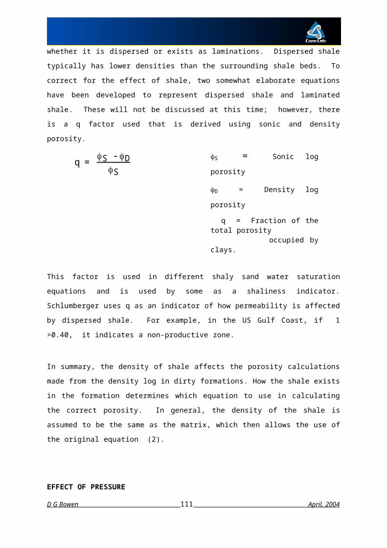
will be calculated. The effect of the shale also depends on whether it is dispersed or exists

as laminations. Dispersed shale typically has lower densities than the surrounding shale

beds. To correct for the effect of shale, two somewhat elaborate equations have been

developed to represent dispersed shale and laminated shale. These will not be discussed

at this time; however, there is a q factor used that is derived using sonic and density

porosity.

q =

S - DS

S = Sonic log porosity

D = Density log porosity

q = Fraction of the total porosity occupied by clays.

This factor is used in different shaly sand water saturation equations and is used by some

as a shaliness indicator. Schlumberger uses q as an indicator of how permeability is

affected by dispersed shale. For example, in the US Gulf Coast, if 1 >0.40, it indicates a

non-productive zone.

In summary, the density of shale affects the porosity calculations made from the density log

in dirty formations. How the shale exists in the formation determines which equation to use

in calculating the correct porosity. In general, the density of the shale is assumed to be the

same as the matrix, which then allows the use of the original equation (2).


EFFECT OF PRESSURE

Increase in depth usually means increase in compaction which causes increase in the bulk

density of shales. This trend, however, is reversed in overpressured zones.

Abnormally high formation pressures are sometimes created due to a sealing off of the

formation and excess water is prevented from escaping. This results in high fluid pressure

which can exceed normal formation pressure. Shales in contact with over pressured

formations contain excess water, are under-compacted, and their bulk densities are lower

than normal. Consequently, the density log can be helpful in predicting the approach to

overpressured zones.

Supplementary Notes


SUMMARY SHEET OF THE DENSITY LOG

A source centrally located on the tool emits gamma rays into the formation. As the

gamma rays enter, they are slowed down and scattered or absorbed. The intensity of

the gamma rays near the detector is recorded.

As porosity decreases, which means the denser the formation, an increase in gamma

rays scattering and absorption occurs; therefore fewer gamma rays are detected. So

the amount of scattering or absorption relates to the formation density which relates to

porosity.

The tool is pressed up against the formation by a pad.

= ma - b

ma - f

The rule of thumb is: If a grain density that is too high is used, a porosity that is too

high will be calculated.

Another rule of thumb is: If a fluid density that is too high is assumed, as in a gas zone

(1.0 gm/cm3 instead of perhaps 0.70 gm/cm3), a porosity that is too high will be

calculate.

Quickie corrections of oil and gas zones are:

for oil T = 0.9D

for gas T = 0.7D

When using the density log in shaly sands, the shale is assumed to have a matrix

density close to 2.65 gm/cm3 and that there is no error. How the shale or clay exists

in the formation, however, does make a difference. Also the type, amount and

hydration of the clay affects the average grain density of the formation.

In a sand containing sodium montmorillonite the average grain density probably should

be lowered. Otherwise, a porosity that is too high will be calculated.


The q factor is used in different shaly sand water saturation equations and also is used

as a permeability indicator:

q =

S - DS

Typically as depth increases so will bulk density. In the overpressured zones, however,

the bulk density of the shales are much lower than expected due to excess water

trapped in the minute pores. This reversal in the trend, if recorded and noticed earlier

enough, can be used to predict abnormally high pressured zones.


STUDY GUIDE QUESTIONS ON THE NEUTRON LOGS

1. Generally, how does the neutron log sense porosity?

2. Name the three basic types of neutron logs?

3. Which logs require liquid? Which logs can be run in cased holes?

4. How are the neutron tools calibrated?

5. How are the neutron logs presented?

6. How do hydrocarbons affect the log response? How can gas be detected?

7. How do clays and other hydrous minerals affect the log response?

8. What elements are resolved by neutron activated geochemical logging?


NEUTRON LOG

INTRODUCTION

Neutrons emitted from a radioactive source are categorised into three general groups

according to their energy:

1. High energy neutrons, which are fast neutrons

2. Medium energy neutrons, which are epithermal neutrons

3. Low energy neutrons, which are thermal neutrons

The logging industry has different tools which respond to different types of these neutrons.

PRINCIPLE

Neutrons are continuously emitted from a source mounted on a down hole tool or device,

often known as a ‘sonde’. These neutrons collide in the formation and lose energy. They

lose the most energy when a nucleus of equal mass is struck. Neutrons have almost equal

mass to protons and only one nucleus consists of a single proton, hydrogen.

Consequently, the amount of neutrons slowed down depends mostly upon the amount of

hydrogen present. This is referred to as the Hydrogen Index (HI) of the formation

Within microseconds of being emitted, the neutrons are slowed down to thermal velocity.

As the neutrons are captured, gamma rays are emitted. Some detectors sense the amount

of gamma rays emitted while others record the density of neutrons in the vicinity of the tool.

If the hydrogen concentration is low in the material surrounding the tool, then the neutron

count rate at the detector will be high; likewise, the opposite is also true. The neutron

count, therefore, reflects the amount of liquid-filled porosity in a clean formation whose

pores are filled with oil and/or water.

TYPES OF TOOLS

The old Conventional Neutron Log (GNT) emitted neutrons from a source in the sonde and

senses the gamma ray intensity around a detector which was spaced 15.5 or 19.5 inches

away. This intensity is roughly proportional to the thermal neutron density and can be

related to porosity. Many factors including the borehole fluid and the tool itself can affect

the reading. Generally, the more gamma rays detected, the less thermal neutrons present;


therefore, more hydrogen is present meaning a higher porosity. This tool is not used

anymore.

The Sidewall Neutron (SNP) is a pad device which detects epithermal neutrons. It has a

detector 16 inches from the source on a pad, which is pressed up against the borehole

wall. The tool can be run in liquid or air-filled uncased holes. The SNP takes the API count

rates, automatically corrects for any borehole irregularities, and then prints the reading in

limestone porosity units. The log senses more than one foot into the formation (depending

upon the hydrogen content) and vertically averages about every 11/2 feet. This tool works

well in complex lithologies. The advantages of the SNP over the GNT are: 1) borehole

effects are minimised, 2) most corrections required are automatically performed, 3)

sensing epithermal neutrons avoids effects of strong thermal neutron absorbers, such as

chlorine and Boron. However, this tool is only rarely used these days.

The Compensated Neutron Log (CNL) has a strong (16 Curie) neutron source and will

detect the amount of thermal neutrons not yet captured by the formation. Two detectors

sufficiently spaced apart (1-2 feet) sense the thermal neutron concentration. The readings

are ratioed, corrections automatically applied, and a compensated porosity curve is derived.

The CNL reads at least 12 inches into the formation. The depth of investigation will vary

according to lithology, porosity, and hydrogen content. This log gives better resolution in

low porosity zones than does the SNP. This tool can be run in either cased or non-cased

liquid-filled holes. The two detectors compensate for borehole irregularities but will not

work well in washed-out zones. The CNL reads deeper than the SNP so it is good for

detecting gas beyond the flushed zone. The CNL is often run in combination with a density

porosity tool.

Modern tools include the DNL, which includes two epi-thermal neutron detectors as well as

the two thermal ones, and the MWD tool, the CDN, which combines a density device within

it. The DNL addresses some of the problems associated with thermal neutron detectors.

The presence of shales and borehole problems may be quantified.

CALIBRATION

The Sidewall and Compensated Neutron Logs are directly calibrated in limestone porosity

units. A test pit standard at the University of Houston is used where the reading from a

19% porosity, water-filled, six feet thick limestone is given as 1000 API units. There are


two other six feet limestone standards of higher (26%) and lower (1.9%) porosities. An

empirical sandstone calibration is available.

The API Calibration Pit For Neutron Porosity

If the matrix is not a limestone, a correction must be made either by built in software, or by

using a porosity correction chart. The correction is developed by using comparisons of


responses in a non-limestone test pit to that in the limestone test pit. This is necessary

because of the different neutron slowing properties of the constitute elements in

sandstones and dolomites. This conversion is now done automatically by the logging unit

and presented with the proper lithology units. However, in mixed lithologies, the calibration

can only be for one component.

Mudcake can affect the sidewall neutron response so corrections are sometimes required.

The compensated neutron log often needs corrections for borehole size, mud weight,

salinity, and temperature-pressure effects. The logging companies, of course, have charts

for these corrections.

THE LOG PRESENTATION

The GNT thermal neutron count rates are plotted on a linear scale typically in tracks three

and four. The SNP computes a porosity and records it directly onto a linearly scaled log,

the CNL is also recorded in linear porosity units. When the CNL is run with another

porosity log, such as the FDC, or LDL, both porosity curves are recorded using the same

scale. This is used to help find gas productive intervals and give a qualitative interpretation

of lithology and porosity. Both the CNL and SNP porosities are presented in limestone

porosity units.


A Neutron Density Log Example

INTERPRETATION

The neutron log is used to identify porous formations and determine their porosity,

distinguish gas from oil or water zones, and when used with other logs, help identify the

lithology. The log works well in carbonates because the clay content is usually low and it

has very good resolution in the lower rang of porosities typically encountered in a

carbonate.

Effects of Hydrocarbons

The tool response depends upon how much hydrogen is present; this is known as the

hydrogen index. The hydrogen index of fresh water is 1.0. Most oils have a hydrogen

index close to one, except light oils and gas; they have lower values due to a lower

hydrogen content. Consequently, the log estimates too low of a porosity in zones

containing gas or light oil. As will be mentioned next, this can be masked by the presence

of adsorbed water in clays.

If the porosity of a zone is fairly constant, a gas liquid contact can be picked using the

neutron log. Gas zones are more easily picked when the neutron and density porosities


are plotted on the same scale. The computed density porosity will read high in gas zones

(a fluid density assumption that is too high would be used) and the neutron log will read

low, therefore, a cross-over will occur. In other words, the density porosity will track to the

left and the neutron porosity will shift to the right. Where they reverse this trend and return

to a more normal response in a porous permeable zone, is an indication of the gas-liquid

contact.

Effect of Shale and Other Hydrous Minerals

It must be remembered that neutron logs sense all of the hydrogen in the formation. That

includes the hydrogen in the oil, the gas, the water, and the crystalline water. This means it

will sense the 48 percent water of crystalinity bound in gypsum crystals and, thus, will

calculate out a porosity too high. This is also true for other hydrous minerals such as opal,

shale or clays in general.

Because gas is not very dense, it has a low hydrogen count which yields too low of a

porosity. In clay-bearing gas productive zones, however, the presence of crystalline water

causes porosities too high and will mask the presence of the gas. How high a neutron

porosity calculates depends upon how much clay is present (and actually what type too).

This concept can be represented mathematically by the equation:


N = T + VSH. NSH N = Observed neutron porosity in a shaly formation

T = True formation porosity

VSH = Volume of the shale

NSH = Neutron porosity of a nearby shale

If a VSH can be determined (the logging manuals cover several ways to estimate it), the

“true” formation porosity without the effect of bound water can be determined. Cross-plots

(i.e., neutron-density) are often used which have the VSH factor incorporated.

Supplementary Notes


GEOCHEMICAL LOGS

GEOCHEMICAL TOOLS, (GLT)

By combining Neutron sources of different energy and the spectral gamma response, it has

become possible to derive the elemental contribution to the activated gamma ray energy

emitted from the formation. At present 12 elements can be derived from their spectra,

these are; aluminium, calcium, chlorine, gadolinium, hydrogen, iron, potassium, silicon,

sulphur, thorium , titanium ,and uranium.

A chemical ‘cook-book’ is applied, assuming that the elements are present as their oxides

and that the oxides concentrations in weight percent sum to unity. Aluminium is derived

from delayed neutron activation analysis, using a californium - 252 source, potassium ,

thorium and uranium are inferred from the relative abundance of their radio-isotopes,

detected by the passive NGS/NGT. The other elements are spectrally derived from the

gamma decay after a burst of 14 MeV neutrons. Magnesium concentrations can be

inferred from the measured Pe, when compared to a derived Pe from the elemental analysis.

Carbon concentrations can also be derived from the carbon-oxygen ratios measured by

gamma-ray spectroscopy by inelastic collisions, utilising the RST, reservoir saturation tool.

Nuclear logging represents a fantastic opportunity to derive a great deal of fundamental

information on the formations of interest. However, there are draw-backs. For accurate

reconstitution of the spectra, it is necessary to develop a training set of mineral responses

within any particular formation. This is usually done by geochemical assay of the

constituent elements making up the rock and requires core samples. These are analysed

by X-ray diffraction, FTIR and mass spectrometry. Once established the mineral set

precision of the approach is very good.

A further draw-back is in the environmental aspects of having portable energetic neutron

sources in a working environment. Tools have to be transported and stored under stringent

regulations. The very latest devices use a new source, which is only activated when under

power.


SUMMARY ON THE NEUTRON LOG

The neutron tool emits neutrons which are slowed down and captured. Different tools

sense wither the amount of neutrons present or the gamma rays emitted after

collision. The quantity detected is dependent upon the amount of hydrogen present.

The amount of hydrogen is dependent upon how much liquid-filled porosity is in the

formation.

The four main tools are:

GNT - The old conventional neutron log which senses thermal neutrons

SNP - The Sidewall Neutron Log, which is a pad device, can be run in

either liquid or air-filled holes, but it can only be run in uncased

holes.

CNL - The Compensated Neutron Log has two detectors that average

the responses which corrects for borehole irregularities. It has a deep

investigation capability and is often run with the density tool to help

detect gas zones. It must be run in liquid-filled holes; however, it

works in cased or uncased holes.

GLT The geo-chemical logging tool has two emitters and three

detectors. It is designed to obtain excitation spectra from

individual elements. One detector is a passive NGS device, the

others look at the gamma-rays from the decay of high energy

neutrons.

These tools are calibrated in the University of Houston’s API test pit which contains

carbonates of known porosities. The porosities are given in limestone porosity units.

If the matrix is not limestone, empirical corrections are made to correlate the porosity

to the proper lithology.

The GNT log presents the API Neutron count rates on a linear scale. Using different

methods of calculation, a porosity can be determined. The SNP and CNL have the

equivalent porosity calculated in the logging unit’s computer and then plotted on a

linear scale.


SUMMARY ON THE NEUTRON LOG (continued)

The neutron log senses porosity fairly well in totally liquid-filled (i.e., not gas or light oil)

formations. Due to less hydrogen present in gas zones, the neutron logs read low.

This anomalous behaviour can be easily detected when a density-neutron log tool is run

and the data is plotted on the same scale. The neutron log will skirt to the right and

the density log will skirt to the left. When they meet again marks the gas-liquid

contact.

There are different methods, to obtain a porosity corrected for the gas effect. Two

popular methods are:

corr = D2 + N

22

corr = ma - b + N

ma

(N as a fraction)

Since the neutron log senses hydrogen, it will also detect the water bound in clay and

other hydratable minerals. Consequently, porosities too high are calculated in

formations containing these types of minerals.


NUCLEAR MAGNETIC RESONANCE, NMR

NMR, or Nuclear Magnetic Resonance was first investigated as a petrophysics tool by

‘Turk’ Timur, at Chevron research, in 1954. However, despite good bench-top apparatus,

which enclosed the sample in a magnetic field, the inverse problem of the field being

enclosed by the sample proved much more difficult to deal with. The earliest down-hole

tools were introduced in 1960 and were not really a success, being phased out of service in

the 1980’s. However, recent advances in the quality of signal generators and detectors

and the use pulse sequences have resulted in a new generation of tools that are, in the

1990s, the most popular in the business.

The NMR Principle

Many nuclei of atoms

have a magnetic moment and they behave like miniature

spinning magnets in the earth’s magnetic field. Hydrogen,

with simply one proton as a nucleus has a relatively large

magnetic moment when compared to the other elemental

nuclei. Fortunately, hydrogen is abundant in water and

hydrocarbon, both fluids. This is important because the

atoms in fluids are free to move in comparison with those


bonded in solid substances. So, we have these spinning protons all aligned in the earth’s

magnetic field. We then create a magnetic field, which is not coincident with that of the

earth. The frequency of this signal is the same as the resonant frequency of hydrogen,

maximising the response. This field is called Bo and is perpendicular to the borehole axis.

A signal is then applied to tilt the nuclei by 90˚ into the B1 direction. The nuclei then precess

in this field, acting like gyroscopes in a gravitational field. This is the basis of the NMR

measurement as this magnetic moment is detected by the tool antennae. Due to small

instabilities in the field, the precessing nuclei begin to dephase, i.e. precess at slightly

different frequencies. As they lose their synchronisation the signal generated decays. The

decay time is called T2 and is petrophysically very important

The decay time T2 actually is dependent on the molecular interactions taking place in the

fluid. The precessing protons have a random flight path and, as they move about, they

collide with other protons and the grain surfaces within the rock. Individual mineral

surfaces have different relaxation properties, but in essence two reactions may occur.

Either the spin energy is lost in the collision and the proton realigns with B0, contributing to

the T1 signal, or the proton is dephased, contributing to the transverse relaxation, T2 signal.

For our work, grain surface relaxation is the primary source of the NMR signal T1 and T2.

Signal Amplitude Processed to Give the T2 Distribution


Grain Surface Relaxation and Pore Size Distribution


As a clear relationship exists between the T2 distribution and the pore-size distribution

there are some corollaries with other petrophysical properties.

NMR Permeability

The relationship between pore size distributions and permeability was investigated by

Burdine in 1953. Following from his work Purcell and others also related capillary held

water saturation to permeability. Kenyon (1988) and Prammer (1994) have proposed

models. The latter of these is called the Timur/Coates formula. The formulae are;

k a 4 (,log

T 2 )2, (Kenyon),

where k is the permeability in millidarcies, is the fractional porosity, a is a formation

dependent constant, typically 4 mD/(ms)2 for Sandstone and 0.4 mD/(ms)2 for carbonates,

and

k a 4 FFI

BFV

2

, (Timur/Coates’)

where FFI is the free fluid index, or moveable fluid volume, and BFV is the bound fluid

volume. The term a’ is a formation dependent constant about 1 x 104 mD for sandstone.

The ‘constants’ above need to be validated by laboratory measurement. However, once

established they can be used within a particular formation with high degrees of confidence.


A Comparison of Core and Log Derived Bound Water T2 Spectra

An Example NMR Log (Schlumberger) Showing High Sw, Mostly

Bound-water

Logging Services

Both Baker Atlas and Schlumberger have NMR tools. With the acquisition of Numar by

Haliburton, HLS now also offer the Numar tools. The Numar - Baker Atlas logs are known

as MRIL and the Schlumberger the CMR. MRIL looks out to 18 inches or so, with a vertical

resolution of 24 inches. The CMR resolves down to 6 inch beds, but depth of investigation

is only about 1 inch.

Precautions

• In order to be absolutely confident in the response another porosity log must be run.

• Medium to high viscosity oil appears as bound fluid.

• Wait-times must be increased in fine, poorly-sorted and tight rocks.

• Low Density shales, coals and tar-mats cause erroneously high free-fluid and

permeability.


cl 2 porosity

Documents