CLAS12 Software

Version 1.3

Editors: D.P. Weygand, V. Ziegler

May 30, 2012

1

Contents

1 The CLAS12 Detector and its Science Program at the Jefferson LabUpgrade 41.1 Introduction . . . . . . . . . . . . . . . . . . . . . . . . . . . . . . . . . . . . 41.2 Science Summary . . . . . . . . . . . . . . . . . . . . . . . . . . . . . . . . . 41.3 From CLAS to CLAS12 . . . . . . . . . . . . . . . . . . . . . . . . . . . . . 51.4 The CLAS12 Detector . . . . . . . . . . . . . . . . . . . . . . . . . . . . . . 6

1.4.1 The Forward Detector . . . . . . . . . . . . . . . . . . . . . . . . . . 71.4.2 The Central Detector . . . . . . . . . . . . . . . . . . . . . . . . . . 8

1.5 Data Acquisition and Trigger . . . . . . . . . . . . . . . . . . . . . . . . . . 91.6 Calibration and Commissioning of CLAS12 . . . . . . . . . . . . . . . . . . 11

2 The CLAS12 Offline Software 142.1 Introduction . . . . . . . . . . . . . . . . . . . . . . . . . . . . . . . . . . . . 142.2 Ways to Increase Productivity . . . . . . . . . . . . . . . . . . . . . . . . . . 152.3 Choice of Computing Model and Architecture . . . . . . . . . . . . . . . . . 152.4 ClaRA: CLAS12 Reconstruction and Analysis Framework . . . . . . . . . . 16

2.4.1 The Attributes of ClaRA Services . . . . . . . . . . . . . . . . . . . 162.4.2 A New Programming Approach . . . . . . . . . . . . . . . . . . . . . 172.4.3 The ClaRA Design Architecture . . . . . . . . . . . . . . . . . . . . 182.4.4 The ClaRA Distribution Environment . . . . . . . . . . . . . . . . . 192.4.5 Performance . . . . . . . . . . . . . . . . . . . . . . . . . . . . . . . 19

2.5 Services . . . . . . . . . . . . . . . . . . . . . . . . . . . . . . . . . . . . . . 222.5.1 Detector Geometry . . . . . . . . . . . . . . . . . . . . . . . . . . . . 222.5.2 Event Display . . . . . . . . . . . . . . . . . . . . . . . . . . . . . . . 222.5.3 Data and Algorithm Services . . . . . . . . . . . . . . . . . . . . . . 242.5.4 Calibration Services . . . . . . . . . . . . . . . . . . . . . . . . . . . 242.5.5 The Magnetic Field Service . . . . . . . . . . . . . . . . . . . . . . . 28

2.6 The CLAS12 Calibration Constants Database . . . . . . . . . . . . . . . . . 29

3 Simulation 303.1 Introduction . . . . . . . . . . . . . . . . . . . . . . . . . . . . . . . . . . . . 30

3.1.1 Parametric Monte Carlo . . . . . . . . . . . . . . . . . . . . . . . . . 303.1.2 CLAS Software with CLAS12 Geometry . . . . . . . . . . . . . . . . . 30

3.2 GEANT4 Monte Carlo: GEMC . . . . . . . . . . . . . . . . . . . . . . . 313.2.1 Main GEMC Features . . . . . . . . . . . . . . . . . . . . . . . . . . 313.2.2 GEMC Detector Geometry . . . . . . . . . . . . . . . . . . . . . . . 313.2.3 CLAS12 Geometry Implementation . . . . . . . . . . . . . . . . . . . 333.2.4 Primary Generator . . . . . . . . . . . . . . . . . . . . . . . . . . . . 363.2.5 Beam(s) Generator . . . . . . . . . . . . . . . . . . . . . . . . . . . . 36

2

3.2.6 Hit Definition . . . . . . . . . . . . . . . . . . . . . . . . . . . . . . . 373.2.7 Hit Process Factory . . . . . . . . . . . . . . . . . . . . . . . . . . . 383.2.8 Elements Identity . . . . . . . . . . . . . . . . . . . . . . . . . . . . . 403.2.9 Output . . . . . . . . . . . . . . . . . . . . . . . . . . . . . . . . . . 413.2.10 Magnetic Fields . . . . . . . . . . . . . . . . . . . . . . . . . . . . . . 413.2.11 Parameters Factory . . . . . . . . . . . . . . . . . . . . . . . . . . . 423.2.12 Material Factory . . . . . . . . . . . . . . . . . . . . . . . . . . . . . 423.2.13 Geometry Factory . . . . . . . . . . . . . . . . . . . . . . . . . . . . 423.2.14 Results . . . . . . . . . . . . . . . . . . . . . . . . . . . . . . . . . . 433.2.15 Documentation . . . . . . . . . . . . . . . . . . . . . . . . . . . . . . 453.2.16 Bug Report . . . . . . . . . . . . . . . . . . . . . . . . . . . . . . . . 453.2.17 Project Management, Code Distribution and Validation . . . . . . . 473.2.18 Project Timeline . . . . . . . . . . . . . . . . . . . . . . . . . . . . . 47

4 Event Reconstruction 484.1 Tracking . . . . . . . . . . . . . . . . . . . . . . . . . . . . . . . . . . . . . . 484.2 Time-of-Flight . . . . . . . . . . . . . . . . . . . . . . . . . . . . . . . . . . 504.3 Cerenkov Counters . . . . . . . . . . . . . . . . . . . . . . . . . . . . . . . . 50

4.3.1 HTCC . . . . . . . . . . . . . . . . . . . . . . . . . . . . . . . . . . . 514.3.2 LTCC . . . . . . . . . . . . . . . . . . . . . . . . . . . . . . . . . . . 52

4.4 Calorimeters . . . . . . . . . . . . . . . . . . . . . . . . . . . . . . . . . . . 544.5 PID for CLAS12 . . . . . . . . . . . . . . . . . . . . . . . . . . . . . . . . . 56

4.5.1 Probability Analysis . . . . . . . . . . . . . . . . . . . . . . . . . . . 56

5 Software Tools 61

6 Post-Reconstruction Data Access 63

7 Online Software 64

8 Code Development and Distribution 658.1 Code Management . . . . . . . . . . . . . . . . . . . . . . . . . . . . . . . . 658.2 Code Release . . . . . . . . . . . . . . . . . . . . . . . . . . . . . . . . . . . 658.3 Software Tracking . . . . . . . . . . . . . . . . . . . . . . . . . . . . . . . . 65

9 Quality Assurance 67

10 Computing Requirements 68

11 Computing Requirements 7411.1 JLab Responsibilities and Institution Responsibilities . . . . . . . . . . . . . 80

3

1 The CLAS12 Detector and its Science Program at theJefferson Lab Upgrade

1.1 Introduction

A brief overview of the CLAS12 detector is presented and a brief synopsis of the initialphysics program after the energy-doubling of the Jefferson Lab electron accelerator. Con-struction of the 12 GeV upgrade project started in October 2008. A broad program hasbeen developed to map the nucleon’s 3-dimensional spin and flavor content through themeasurement of deeply exclusive and semi-inclusive processes. Other programs includemeasurements of the forward distribution function to large xB ≤ 0.85 and the quark andgluon polarized distribution functions, and nucleon ground state and transition form fac-tors at high Q2. The 12 GeV electron beam and the large acceptance of CLAS12 are alsowell suited to explore hadronization properties using the nucleus as a laboratory.

1.2 Science Summary

The challenge of understanding nucleon electromagnetic structure still continues after morethan five decades of experimental scrutiny. From the initial measurements of elastic formfactors to the accurate determination of parton distributions through deep inelastic scat-tering (DIS), the experiments have increased in statistical and systematic accuracy. It wasrealized in recent years that the parton distribution functions represent special cases of amore general and much more powerful way of characterizing the structure of the nucleon,the generalized parton distributions (GPDs).

The GPDs describe the simultaneous distribution of particles with respect to bothposition and momentum. In addition to providing information about the spatial density(form factors) and momentum density (parton distributions), these functions reveal thecorrelation of the spatial and momentum distributions, i.e. how the spatial shape of thenucleon changes when probing quarks of different wavelengths.

The concept of GPDs has led to completely new methods of “spatial imaging” of thenucleon, either in the form of two-dimensional tomographic images, or in the form ofgenuine three-dimensional images. GPDs also allow us to quantify how the orbital motionof quarks in the nucleon contributes to the nucleon spin – a question of crucial importancefor our understanding of the “mechanics” underlying nucleon structure. The spatial viewof the nucleon enabled by the GPDs provides us with new ways to test dynamical modelsof nucleon structure.

The mapping of the nucleon GPDs, and a detailed understanding of the spatial quarkand gluon structure of the nucleon, have been widely recognized as the key objectives ofnuclear physics of the next decade. This requires a comprehensive program, combiningresults of measurements of a variety of processes in electron–nucleon scattering with struc-tural information obtained from theoretical studies, as well as with expected results from

4

future lattice QCD simulations.While GPDs, and also the more recently introduced transverse momentum-dependent

distribution functions (TMDs), open up new avenues of research, the traditional means ofstudying nucleon structure through electromagnetic elastic and transition form factors, andthrough flavor- and spin-dependent parton distributions, must also be employed with highprecision to extract physics on the nucleon structure in the transition from the regime ofquark confinement to the domain of asymptotic freedom. These avenues of research can beexplored using the 12 GeV cw beam of the JLab upgrade with much higher precision thanhas been achieved before, and can help reveal some of the remaining secrets of QCD. Also,the high luminosity available will allow researchers to explore the regime of extreme quarkmomentum, where a single quark carries 80% or more of the proton’s total momentum.This domain of QCD has been hardly explored and provides challenges to the detectionsystems in term of kinematic coverage and high luminosity operation.

A large portion of the science program is dedicated to the measurement of exclusiveprocesses, such as deeply virtual Compton scattering ep → epγ or deeply virtual mesonproduction, e.g. ep→ epρ0 or ep→ eπ+n, which require the detection of 3 or 4 particles inthe final state. Another part of the program is based on the measurement of semi-inclusiveprocesses, e.g. ep → eπ+X or ep → eπ0X, where a high momentum charged or neutralpion must be detected in addition to the scattered electron.

Other programs require measurement of the full cm angular distribution of a morecomplex final state such as ep → epπ+π− to be able to identify the spin-parity of anintermediate baryon resonance.

The CLAS12 science program currently covers GDPs, hard-exclusive processes, semi-inclusive deep inelastic processes, single-spin asymmetry measurements, deep inelasticstructure functions of the nucleon, experiments using the nucleus as a laboratory andhadron spectroscopy. It includes a broad program using polarized beams, longitudinallyand transversely polarized targets, and measurements of outgoing recoil baryon polariza-tion.

1.3 From CLAS to CLAS12

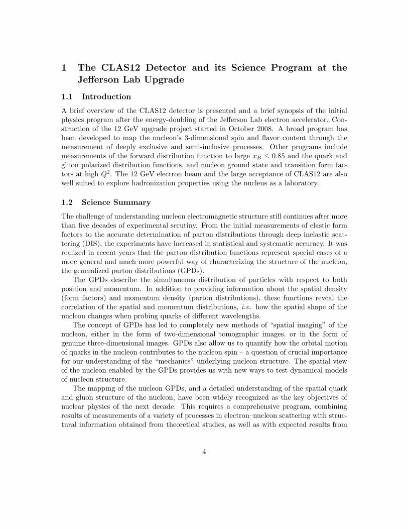
The CLAS detector was designed and built in the 1990s and became fully operational in1998. It has been in operation since. CLAS has been operated with electron and photonbeams with luminosities up to L = 1034 sec−1cm−2. The driving motivation for CLASwas the nucleon resonance program, with emphasis on the study of resonance transitionform factors and the search for missing resonances. Figure 1 shows two schematic viewsof CLAS. At the core of CLAS is a toroidal magnet consisting of six superconductingcoils symmetrically arranged around the beam line. Each of the sectors is instrumentedas an independent spectrometer with 34 layers of tracking chambers, allowing for the fullreconstruction of the charged particle 3-momentum vectors. Charged hadron identificationis accomplished by combining momentum and time-of-flight with the measured path length

5

from the target to the scintillation counters which surround the tracking detectors. Theforward angular range from 10◦ to 50◦ is instrumented with gas Cerenkov counters for theidentification of electrons.

The CLAS data acquisition system was designed to read out 35,000 drift chamber sensewires and over 2,500 channels of photomultiplier tubes.

Drift ChambersRegion 1Region 2Region 3

TOF Counters Cerenkov Counters

Large-angle CalorimeterElectromagnetic Calorimeter

1 m

Drift ChambersRegion 1Region 2Region 3

TOF Counters

Main Torus Coils

Mini-torus Coils1 m

Figure 1: Two views of the CLAS detector system. Left panel: Longitudinal cut alongthe beam line showing the three different regions of drift chambers, the Cerenkov countersat forward angles, the time-of-flight (TOF) system, and the electromagnetic calorimeters.The simulated event shows an electron (upper) and a positively charged hadron. Rightpanel: Transverse cut through CLAS. The six superconducting coils provide a six sectorstructure with independent detectors.

1.4 The CLAS12 Detector

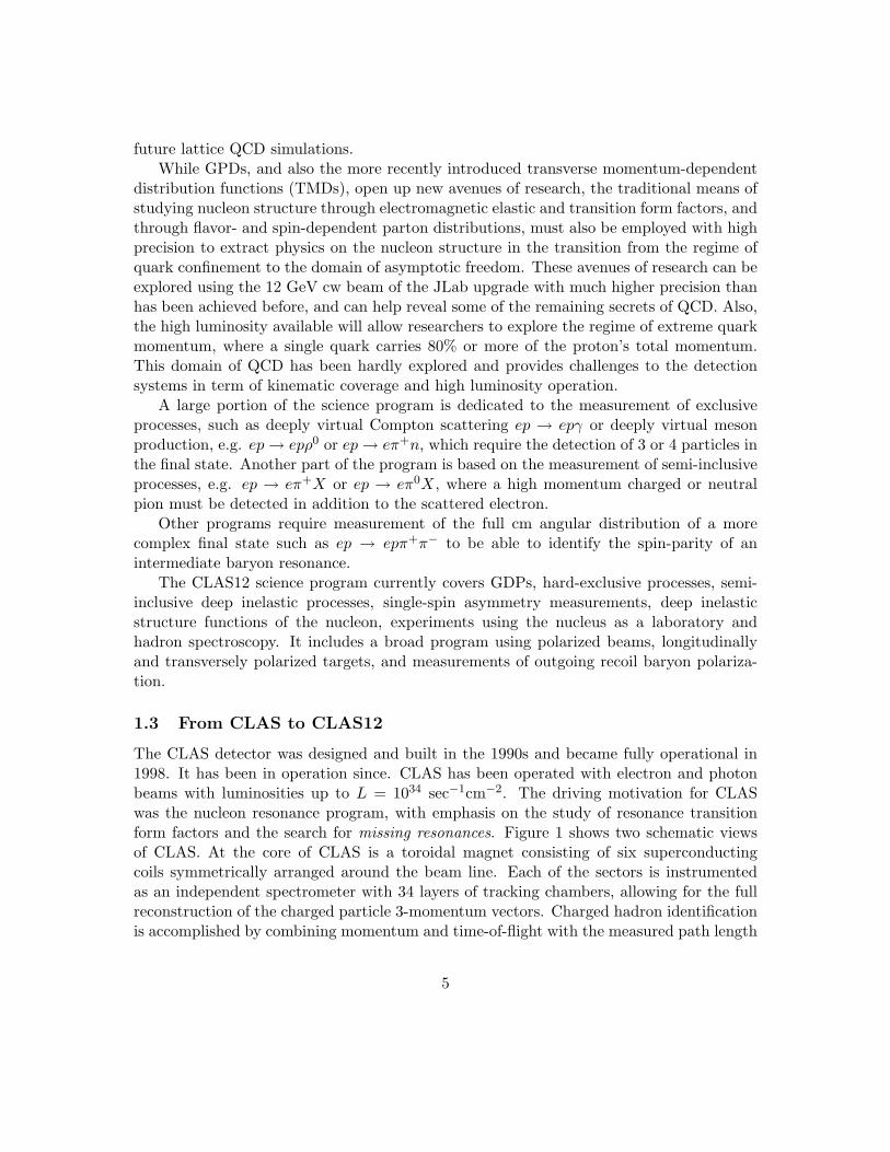
To meet the requirements of high statistics measurements for exclusive processes, the equip-ment at JLab will undergo major upgrades. In particular it will include the CLAS12 LargeAcceptance Spectrometer [1]. A 3-dimensional rendition is shown in Fig. 2. CLAS12 hastwo major parts with different functions, the Forward Detector (FD) and the Central De-tector (CD). The FD retains the 6-sector symmetric design of CLAS, which is based ona toroidal magnet with six superconducting coils that are symmetrically arranged aroundthe beam axis. The main new features of CLAS12 include operation with a luminosityof 1035 cm−2sec−1, an order of magnitude increase over CLAS [2], and improved accep-tance and particle detection capabilities at forward angles. In this section we present short

6

descriptions of the detector system.

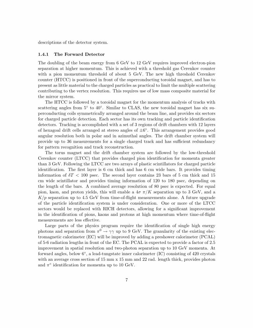
1.4.1 The Forward Detector

The doubling of the beam energy from 6 GeV to 12 GeV requires improved electron-pionseparation at higher momentum. This is achieved with a threshold gas Cerenkov counterwith a pion momentum threshold of about 5 GeV. The new high threshold Cerenkovcounter (HTCC) is positioned in front of the superconducting toroidal magnet, and has topresent as little material to the charged particles as practical to limit the multiple scatteringcontributing to the vertex resolution. This requires use of low mass composite material forthe mirror system.

The HTCC is followed by a toroidal magnet for the momentum analysis of tracks withscattering angles from 5◦ to 40◦. Similar to CLAS, the new toroidal magnet has six su-perconducting coils symmetrically arranged around the beam line, and provides six sectorsfor charged particle detection. Each sector has its own tracking and particle identificationdetectors. Tracking is accomplished with a set of 3 regions of drift chambers with 12 layersof hexagoal drift cells arranged at stereo angles of ±6◦. This arrangement provides goodangular resolution both in polar and in azimuthal angles. The drift chamber system willprovide up to 36 measurements for a single charged track and has sufficient redundancyfor pattern recognition and track reconstruction.

The torus magnet and the drift chamber system are followed by the low-thresholdCerenkov counter (LTCC) that provides charged pion identification for momenta greaterthan 3 GeV. Following the LTCC are two arrays of plastic scintillators for charged particleidentification. The first layer is 6 cm thick and has 6 cm wide bars. It provides timinginformation of δT < 100 psec. The second layer contains 23 bars of 5 cm thick and 15cm wide scintillator and provides timing information of 120 to 180 psec, depending onthe length of the bars. A combined average resolution of 80 psec is expected. For equalpion, kaon, and proton yields, this will enable a 4σ π/K separation up to 3 GeV, and aK/p separation up to 4.5 GeV from time-of-flight measurements alone. A future upgradeof the particle identification system is under consideration. One or more of the LTCCsectors would be replaced with RICH detectors, allowing for a significant improvementin the identification of pions, kaons and protons at high momentum where time-of-flightmeasurements are less effective.

Large parts of the physics program require the identification of single high energyphotons and separation from π0 → γγ up to 9 GeV. The granularity of the existing elec-tromagnetic calorimeter (EC) will be improved by adding a preshower calorimeter (PCAL)of 5-6 radiation lengths in front of the EC. The PCAL is expected to provide a factor of 2.5improvement in spatial resolution and two-photon separation up to 10 GeV momenta. Atforward angles, below 6◦, a lead-tungstate inner calorimeter (IC) consisting of 420 crystalswith an average cross section of 15 mm x 15 mm and 22 rad. length thick, provides photonand π◦ identification for momenta up to 10 GeV.

7

A quasi-real photon forward tagging system (FT) will measure electrons at scatter-ing angles from 2◦ - 4◦ using the IC for energy measurements, a segmented scintillatorhodoscope for triggering, and micromegas tracking chambers.

1.4.2 The Central Detector

The Central Detector (CD) is based on a compact solenoid magnet with maximum centralmagnetic field of 5 Tesla. The solenoid magnet provides momentum analysis for polarangles greater than 35◦, protection of the tracking detectors from background electrons, andacts as a polarizing field for dynamically polarized solid state targets. All three functionsrequire high magnetic field. The overall size of the solenoid is restricted to 2000 mm indiameter, which allows a maximum warm bore for the placement of detectors of 780 mm.To obtain sufficient momentum resolution in the limited space available requires high fieldand excellent position resolution of the tracking detectors. The central field in the targetregion must also be very uniform at ∆B/B < 10−4 to allow the operation of a dynamicallypolarized target. To achieve a sustained high polarization for polarized ammonia targetsrequires magnetic fields in excess of 3 T. Magnetic fields of 5 T have been most recently usedfor such targets with polarization of 80% - 90% for hydrogen. In addition, the solenoidalfield provides the ideal guiding field for keeping the copiously produced Moller electronsaway from the sensitive detectors and guide them to downstream locations where they canbe passively absorbed in high-Z material. The production target is centered in the solenoidmagnet. A forward micromegas tracker (FMT) consisting of 6 stereo layers is located justdownstream of the production target and in front of the HTCC. The FMT aids the trackreconstruction in the FD and covers the polar angle range of 5◦ to 35◦ and improves vertexand momentum resolution of high momentum tracks.

Tracking in the CD is provided by a silicon vertex tracker (SVT) and a barrel mi-cromegas tracker (BMT). Each of the two detectors provide 3 space points for the tracksin the angle range of the CD. The combined SVT and BMT cover polar angles from 35◦

to 125◦.The central time-of-flight scintillator barrel (CTOF) consists of 48 bars of fast plastic

scintillator equipped with 96 photomultiplier tubes that provide 2-sided light read-out.The scintillator light is brought to an area of reduced magnetic field where fast PMTswith dynamical shielding arrangement can be employed. A timing resolution of less than60 psec has been achieved for this system in prototype tests. The very short flight pathavailable in the CD allows for particle identification in a restricted momentum range of upto 1.2 GeV and 0.65 GeV for pion-proton and pion-kaon separation, respectively.

Also under development by a French-Italian collaboration is an additional detector thatwill add neutral particle detection capabilities. This detector will fill the gap between theCTOF and the solenoid cryostat.

With these upgrades CLAS12, will be the workhorse for exclusive and semi-inclusiveelectro-production experiments in the deep inelastic kinematics.

8

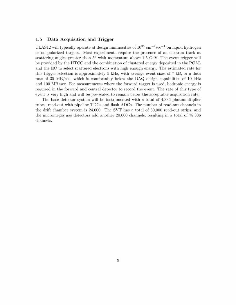
1.5 Data Acquisition and Trigger

CLAS12 will typically operate at design luminosities of 1035 cm−2sec−1 on liquid hydrogenor on polarized targets. Most experiments require the presence of an electron track atscattering angles greater than 5◦ with momentum above 1.5 GeV. The event trigger willbe provided by the HTCC and the combination of clustered energy deposited in the PCALand the EC to select scattered electrons with high enough energy. The estimated rate forthis trigger selection is approximately 5 kHz, with average event sizes of 7 kB, or a datarate of 35 MB/sec, which is comfortably below the DAQ design capabilities of 10 kHzand 100 MB/sec. For measurements where the forward tagger is used, hadronic energy isrequired in the forward and central detector to record the event. The rate of this type ofevent is very high and will be pre-scaled to remain below the acceptable acquisition rate.

The base detector system will be instrumented with a total of 4,336 photomultipliertubes, read-out with pipeline TDCs and flash ADCs. The number of read-out channels inthe drift chamber system is 24,000. The SVT has a total of 30,000 read-out strips, andthe micromegas gas detectors add another 20,000 channels, resulting in a total of 78,336channels.

9

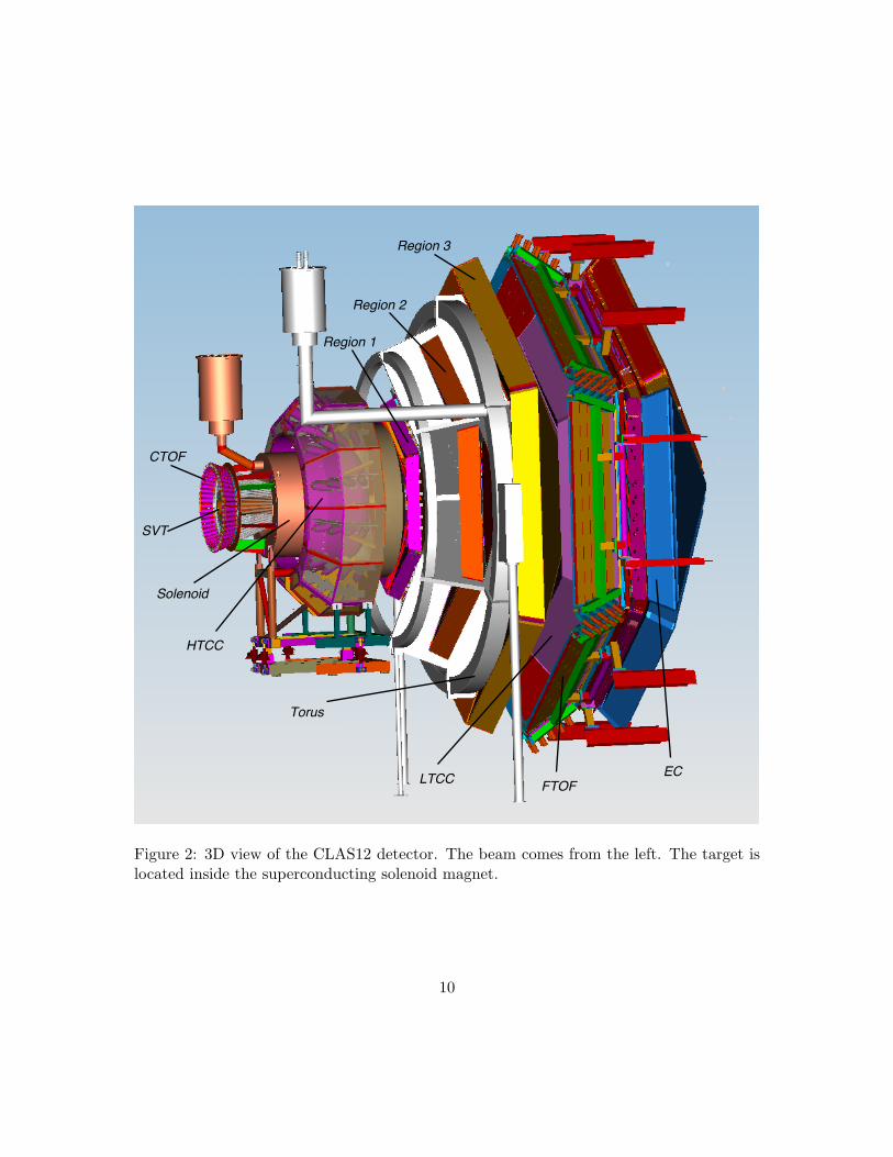
CTOF

SVT

FTOF

HTCC

Solenoid

LTCC

Torus

EC

Region 1

Region 2

Region 3

Figure 2: 3D view of the CLAS12 detector. The beam comes from the left. The target islocated inside the superconducting solenoid magnet.

10

1.6 Calibration and Commissioning of CLAS12

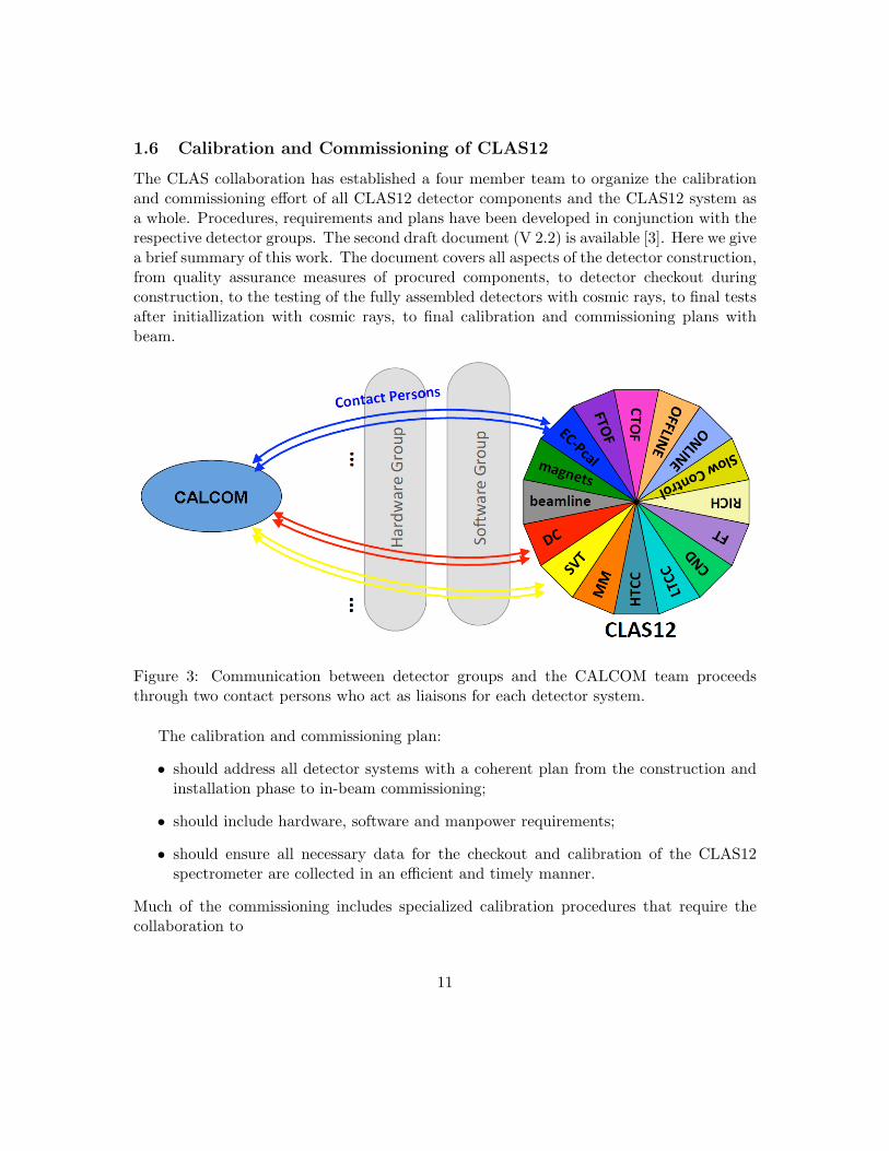
The CLAS collaboration has established a four member team to organize the calibrationand commissioning effort of all CLAS12 detector components and the CLAS12 system asa whole. Procedures, requirements and plans have been developed in conjunction with therespective detector groups. The second draft document (V 2.2) is available [3]. Here we givea brief summary of this work. The document covers all aspects of the detector construction,from quality assurance measures of procured components, to detector checkout duringconstruction, to the testing of the fully assembled detectors with cosmic rays, to final testsafter initiallization with cosmic rays, to final calibration and commissioning plans withbeam.

Figure 3: Communication between detector groups and the CALCOM team proceedsthrough two contact persons who act as liaisons for each detector system.

The calibration and commissioning plan:

• should address all detector systems with a coherent plan from the construction andinstallation phase to in-beam commissioning;

• should include hardware, software and manpower requirements;

• should ensure all necessary data for the checkout and calibration of the CLAS12spectrometer are collected in an efficient and timely manner.

Much of the commissioning includes specialized calibration procedures that require thecollaboration to

11

• develop and test procedures for each detector system;

• define input data (data type and statistics) for the calibration algorithms;

• develop and test the necessary software tools;

• evaluate manpower and computing resource needs;

• provide all relevant parameters to perform full reconstruction and to evaluate thedetector performance.

An important mechanism in this process is the CLAS12 Service Work Committee to whichall collaborating institutions provide manpower resources: graduate student, postdocs, andsenior researchers who pledge to devote part of their time in general support of the collab-oration’s goals through software or hardware contributions. The CALCOM group receivesrequests from the detector groups via two liaison persons for support with calibration, com-missioning, and maintenance activities. The CALCOM group can then request resourcesfrom the Service Work Committee to assign the necessary resources to support a specificdetector group. Figure 3 illustrates schematically the relationship between the detectorgroups and the CALCOM committee. The detector groups develop their own softwareneeded for the calibration and commissioning tasks, much of which will be re-used afterthe detector installation in CLAS12, including during beam operation. Representativefigures of the PCAL calibration procedure during cosmic ray testing are shown in Fig. 4.

12

PCAL  Checkout  and  Calibra4on  Full  checkout/calibra0on  of  first  sector  module  with  cosmic  rays  •  PMT  gain  matching  •  Light  a>enua0on  •  Light  Yield  (in  progress)  Full  detector  calibra0on  

Figure 4: Calibration procedures during the cosmic ray testing of one of the six pre-showercalorimeter modules. The PMT signals are analyzed with the online software to determinethe attenuation length of each scintillator stack and for gain matching. The ADC spectrashow the fully calibrated and gain-matched detector response.

13

2 The CLAS12 Offline Software

2.1 Introduction

Modern high energy and nuclear physics experiments require significant computing powerto keep up with large experimental data volumes. To achieve quality physics data anal-ysis, intellectual input from diverse groups within a large collaboration must be broughttogether.

Experimental physics data analysis in a collaborative environment has historically in-volved a computing model based on self-contained, monolithic software applications run-ning in batch-processing mode. This model, if not organized properly, can result in inef-ficiencies in terms of deployment, maintenance, response to program errors, update prop-agation, scalability and fault-tolerance. We have experienced such problems during thefifteen years of operation of the CLAS on- and off-line software. Even though these chal-lenges are common to all physics data processing (PDP) applications, the small size of theCLAS offline group magnified their effect. Experimental configurations have become morecomplex and compute capacity has expanded at a rate consistent with Moore’s Law. As aconsequence, these compute applications have become much more complex, with significantinteraction between diverse program components. This has led to computing systems socomplex and intertwined that the programs have become difficult to maintain and extend.

In large experimental physics collaborations it is difficult to enforce policies on computerhardware. For example, some groups might use whatever computing resources they haveat their home institutions. In turn, these resources evolve as new hardware is added.Additional software and organizational effort must often be put in place to provide themaintenance needed to update and rebuild software applications for proper functionalityin specific hardware or OS environments.

In order to improve productivity, it is essential to provide location-independent ac-cess to data, as well as flexibility of the design, operation, maintenance and extension ofphysics data processing applications. Physics data processing applications have a verylong lifetime, and the ability to upgrade technologies is therefore essential. Thus, softwareapplications must be organized in a way that easily permits the discarding of aged com-ponents and the inclusion of new ones without having to redesign entire software packagesat each change. The addition of new modules and removal of unsatisfactory ones is anatural process of the evolution of applications over time. Experience shows that softwareevolution and diversification is important, and results in more efficient and robust applica-tions. New generations of young physicists doing data analysis may or may not have theprogramming skills required for extending/modifying applications that were written usingolder technologies. For example, JAVA is the main educational programming language inmany universities today, but most of the data production software applications are writtenin C++ and some even in FORTRAN.

The offline software of the CLAS12 project aims at providing tools to the collaboration

14

that allow design, simulation, and data analysis to proceed in an efficient, repeatable,and understandable way. The process should be designed to minimize errors and to allowcross-checks of results. As much as possible, software-engineering-related details should behidden from collaborators, allowing them to concentrate on the physics.

2.2 Ways to Increase Productivity

There are well-known practices leading to improved software productivity and quality.These include software modularity, minimized coupling and dependencies between mod-ules, simplicity and operational specialization of modules, technology abstraction (includinghigh level programming languages), and most importantly, rapid prototyping, deploymentand testing cycles. It is also important to take into account the qualifications of soft-ware contributors: the physicist best understands the physics process and algorithms, andthe computer scientist/programmer has advanced skills in software programming. An en-vironment that encourages collaboration, with code development responsibilities clearlyseparated and established, can increase the quality and number of physics data analysiscontributions. The CLAS12 software group has studied different PDP frameworks and hassearched for contemporary approaches and computing architectures best suited to achievethese goals. The CLAS12 framework design was inspired to a great extent by the GAUDIframework [4] which was adopted by the LHCb experiment. The CLAS12 frameworkincludes design concepts based on the GAUDI framework’s data centricity, its clear sep-aration between data and algorithms, and its data classifications. However, the GAUDIframework is based on an Object Oriented Architecture (OOA), requiring compilation ina self-contained, monolithic application that can only be scaled in batch or grid systems.This approach usually requires that a relatively large software group be involved in thedevelopment, maintenance and system operation.

2.3 Choice of Computing Model and Architecture

We have researched among the most advanced emerging computing trends and our at-tention was caught by the cloud-computing model. This model promises to address ourcomputing challenges. It has reached its maturity level and many scientific organizations,including CERN, are moving in its direction. The cloud computing model is based on aService Oriented Architecture (SOA). SOA is a way of designing, developing, deploying andmanaging software systems characterized by coarse-grained services that represent reusablefunctionality. In SOA, service consumers compose applications or systems using the func-tionality provided by these services through a standard interface. SOA is not a technologyand is more like a blueprint for designing and developing computational environments. Ser-vices usually are loosely coupled, depending on each other minimally. Services encapsulateand hide technologies, as well as the functional contexts used inside a service.

15

2.4 ClaRA: CLAS12 Reconstruction and Analysis Framework

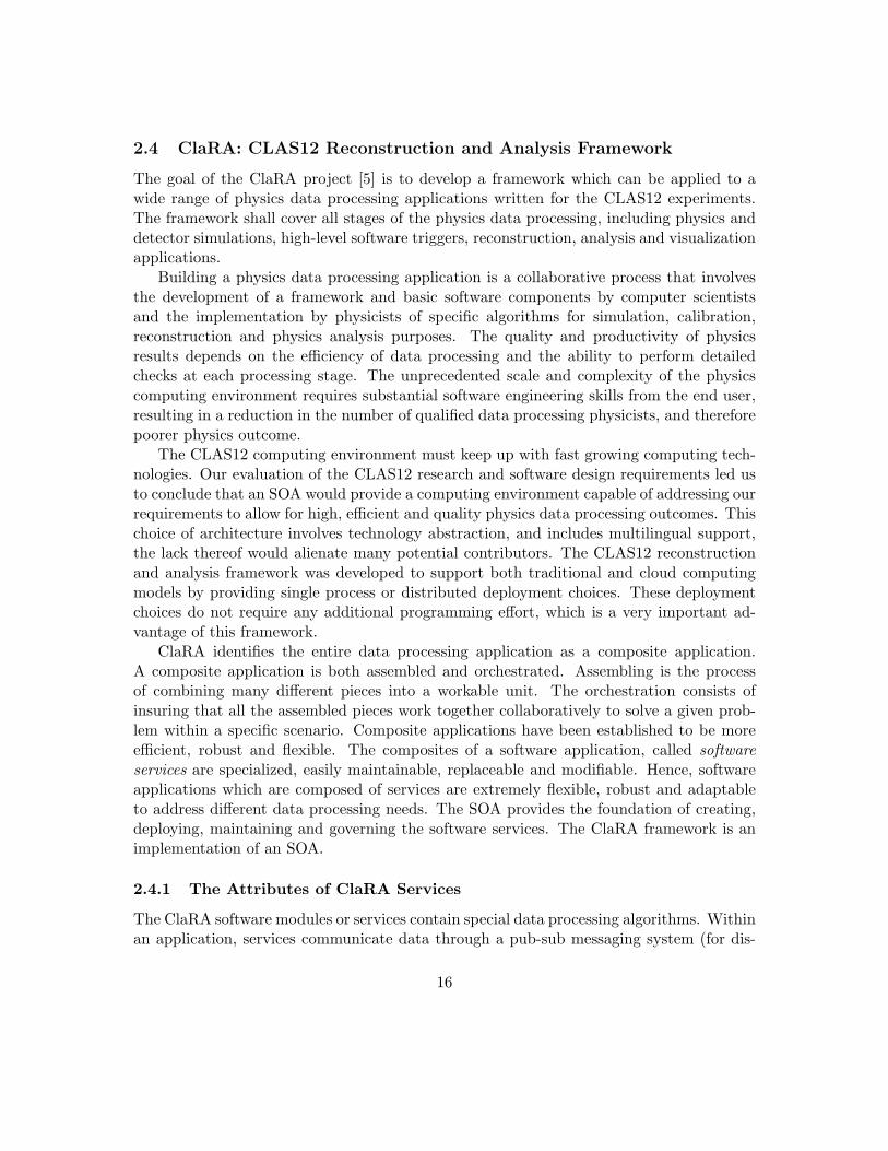
The goal of the ClaRA project [5] is to develop a framework which can be applied to awide range of physics data processing applications written for the CLAS12 experiments.The framework shall cover all stages of the physics data processing, including physics anddetector simulations, high-level software triggers, reconstruction, analysis and visualizationapplications.

Building a physics data processing application is a collaborative process that involvesthe development of a framework and basic software components by computer scientistsand the implementation by physicists of specific algorithms for simulation, calibration,reconstruction and physics analysis purposes. The quality and productivity of physicsresults depends on the efficiency of data processing and the ability to perform detailedchecks at each processing stage. The unprecedented scale and complexity of the physicscomputing environment requires substantial software engineering skills from the end user,resulting in a reduction in the number of qualified data processing physicists, and thereforepoorer physics outcome.

The CLAS12 computing environment must keep up with fast growing computing tech-nologies. Our evaluation of the CLAS12 research and software design requirements led usto conclude that an SOA would provide a computing environment capable of addressing ourrequirements to allow for high, efficient and quality physics data processing outcomes. Thischoice of architecture involves technology abstraction, and includes multilingual support,the lack thereof would alienate many potential contributors. The CLAS12 reconstructionand analysis framework was developed to support both traditional and cloud computingmodels by providing single process or distributed deployment choices. These deploymentchoices do not require any additional programming effort, which is a very important ad-vantage of this framework.

ClaRA identifies the entire data processing application as a composite application.A composite application is both assembled and orchestrated. Assembling is the processof combining many different pieces into a workable unit. The orchestration consists ofinsuring that all the assembled pieces work together collaboratively to solve a given prob-lem within a specific scenario. Composite applications have been established to be moreefficient, robust and flexible. The composites of a software application, called softwareservices are specialized, easily maintainable, replaceable and modifiable. Hence, softwareapplications which are composed of services are extremely flexible, robust and adaptableto address different data processing needs. The SOA provides the foundation of creating,deploying, maintaining and governing the software services. The ClaRA framework is animplementation of an SOA.

2.4.1 The Attributes of ClaRA Services

The ClaRA software modules or services contain special data processing algorithms. Withinan application, services communicate data through a pub-sub messaging system (for dis-

16

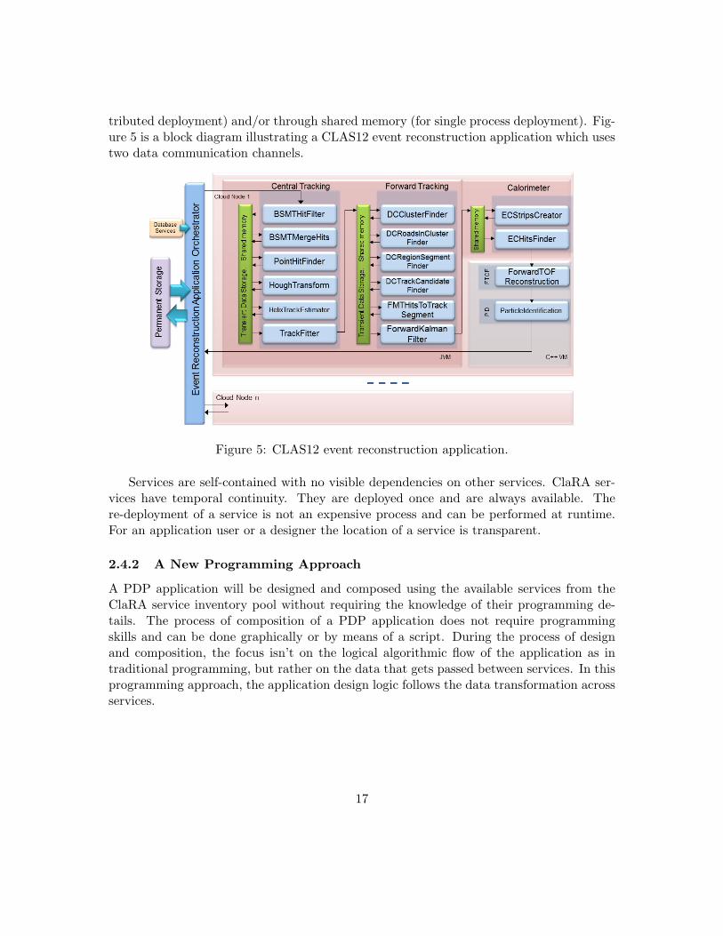
tributed deployment) and/or through shared memory (for single process deployment). Fig-ure 5 is a block diagram illustrating a CLAS12 event reconstruction application which usestwo data communication channels.

Figure 5: CLAS12 event reconstruction application.

Services are self-contained with no visible dependencies on other services. ClaRA ser-vices have temporal continuity. They are deployed once and are always available. There-deployment of a service is not an expensive process and can be performed at runtime.For an application user or a designer the location of a service is transparent.

2.4.2 A New Programming Approach

A PDP application will be designed and composed using the available services from theClaRA service inventory pool without requiring the knowledge of their programming de-tails. The process of composition of a PDP application does not require programmingskills and can be done graphically or by means of a script. During the process of designand composition, the focus isn’t on the logical algorithmic flow of the application as intraditional programming, but rather on the data that gets passed between services. In thisprogramming approach, the application design logic follows the data transformation acrossservices.

17

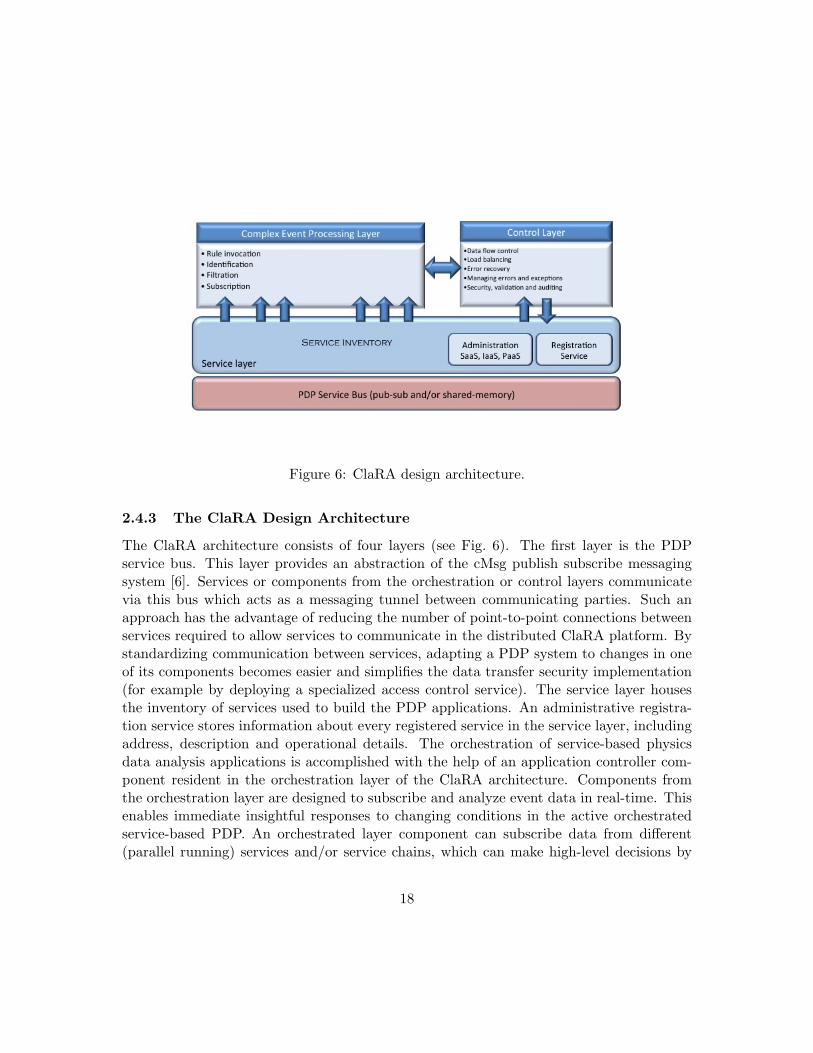
Figure 6: ClaRA design architecture.

2.4.3 The ClaRA Design Architecture

The ClaRA architecture consists of four layers (see Fig. 6). The first layer is the PDPservice bus. This layer provides an abstraction of the cMsg publish subscribe messagingsystem [6]. Services or components from the orchestration or control layers communicatevia this bus which acts as a messaging tunnel between communicating parties. Such anapproach has the advantage of reducing the number of point-to-point connections betweenservices required to allow services to communicate in the distributed ClaRA platform. Bystandardizing communication between services, adapting a PDP system to changes in oneof its components becomes easier and simplifies the data transfer security implementation(for example by deploying a specialized access control service). The service layer housesthe inventory of services used to build the PDP applications. An administrative registra-tion service stores information about every registered service in the service layer, includingaddress, description and operational details. The orchestration of service-based physicsdata analysis applications is accomplished with the help of an application controller com-ponent resident in the orchestration layer of the ClaRA architecture. Components fromthe orchestration layer are designed to subscribe and analyze event data in real-time. Thisenables immediate insightful responses to changing conditions in the active orchestratedservice-based PDP. An orchestrated layer component can subscribe data from different(parallel running) services and/or service chains, which can make high-level decisions by

18

correlating multiple events (for example particle identification, triggers, etc.).

2.4.4 The ClaRA Distribution Environment

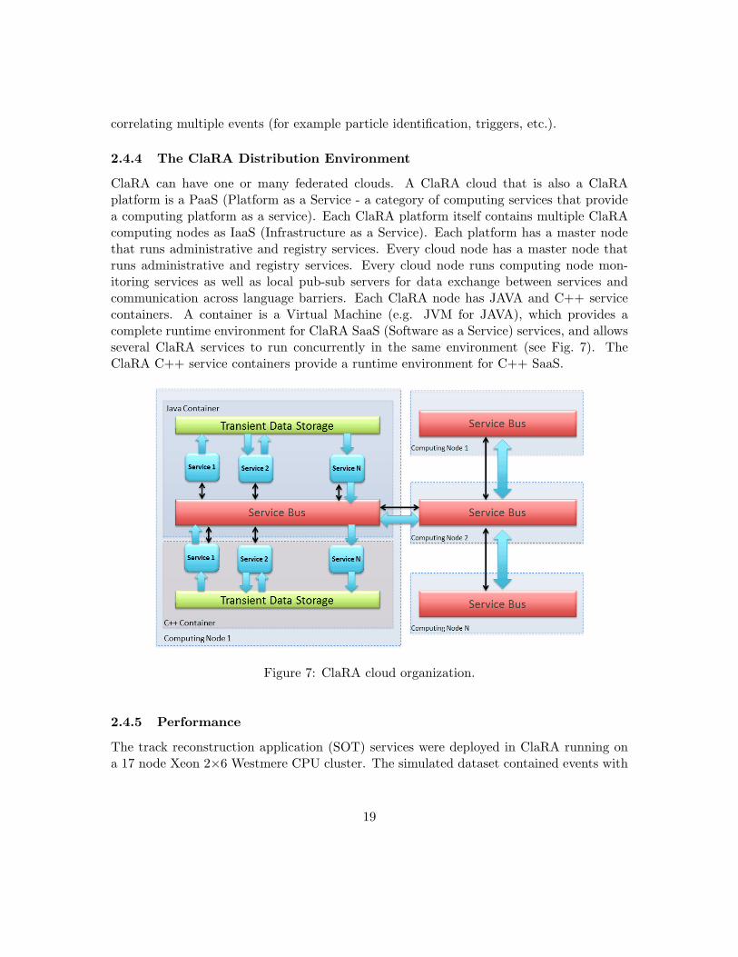
ClaRA can have one or many federated clouds. A ClaRA cloud that is also a ClaRAplatform is a PaaS (Platform as a Service - a category of computing services that providea computing platform as a service). Each ClaRA platform itself contains multiple ClaRAcomputing nodes as IaaS (Infrastructure as a Service). Each platform has a master nodethat runs administrative and registry services. Every cloud node has a master node thatruns administrative and registry services. Every cloud node runs computing node mon-itoring services as well as local pub-sub servers for data exchange between services andcommunication across language barriers. Each ClaRA node has JAVA and C++ servicecontainers. A container is a Virtual Machine (e.g. JVM for JAVA), which provides acomplete runtime environment for ClaRA SaaS (Software as a Service) services, and allowsseveral ClaRA services to run concurrently in the same environment (see Fig. 7). TheClaRA C++ service containers provide a runtime environment for C++ SaaS.

Figure 7: ClaRA cloud organization.

2.4.5 Performance

The track reconstruction application (SOT) services were deployed in ClaRA running ona 17 node Xeon 2×6 Westmere CPU cluster. The simulated dataset contained events with

19

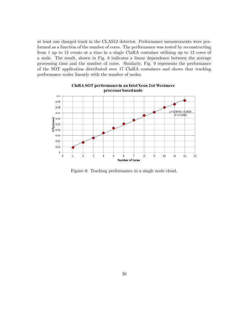
at least one charged track in the CLAS12 detector. Performance measurements were per-formed as a function of the number of cores. The performance was tested by reconstructingfrom 1 up to 12 events at a time in a single ClaRA container utilizing up to 12 cores ofa node. The result, shown in Fig. 8 indicates a linear dependence between the averageprocessing time and the number of cores. Similarly, Fig. 9 represents the performanceof the SOT application distributed over 17 ClaRA containers and shows that trackingperformance scales linearly with the number of nodes.

Figure 8: Tracking performance in a single node cloud.

20

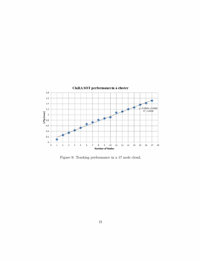
Figure 9: Tracking performance in a 17 node cloud.

21

2.5 Services

This section details the various services of the ClaRA framwork.

2.5.1 Detector Geometry

The Geometry service is an example of a detector data service. This is the front-end of theCLAS12 geometry data, encapsulating data access and data management details from theservice consumers. All the ClaRA algorithm services, including simulation, reconstruction,alignment, and calibration will access the geometry service using standard service commu-nication protocols, provided by the framework. Currently geometry information is storedin a mySQL database and will be part of the calibration database.

2.5.2 Event Display

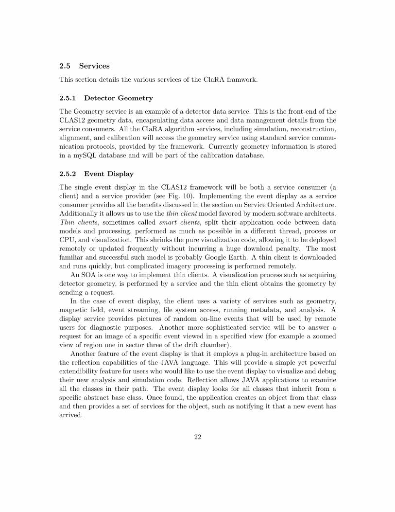
The single event display in the CLAS12 framework will be both a service consumer (aclient) and a service provider (see Fig. 10). Implementing the event display as a serviceconsumer provides all the benefits discussed in the section on Service Oriented Architecture.Additionally it allows us to use the thin client model favored by modern software architects.Thin clients, sometimes called smart clients, split their application code between datamodels and processing, performed as much as possible in a different thread, process orCPU, and visualization. This shrinks the pure visualization code, allowing it to be deployedremotely or updated frequently without incurring a huge download penalty. The mostfamiliar and successful such model is probably Google Earth. A thin client is downloadedand runs quickly, but complicated imagery processing is performed remotely.

An SOA is one way to implement thin clients. A visualization process such as acquiringdetector geometry, is performed by a service and the thin client obtains the geometry bysending a request.

In the case of event display, the client uses a variety of services such as geometry,magnetic field, event streaming, file system access, running metadata, and analysis. Adisplay service provides pictures of random on-line events that will be used by remoteusers for diagnostic purposes. Another more sophisticated service will be to answer arequest for an image of a specific event viewed in a specified view (for example a zoomedview of region one in sector three of the drift chamber).

Another feature of the event display is that it employs a plug-in architecture based onthe reflection capabilities of the JAVA language. This will provide a simple yet powerfulextendibility feature for users who would like to use the event display to visualize and debugtheir new analysis and simulation code. Reflection allows JAVA applications to examineall the classes in their path. The event display looks for all classes that inherit from aspecific abstract base class. Once found, the application creates an object from that classand then provides a set of services for the object, such as notifying it that a new event hasarrived.

22

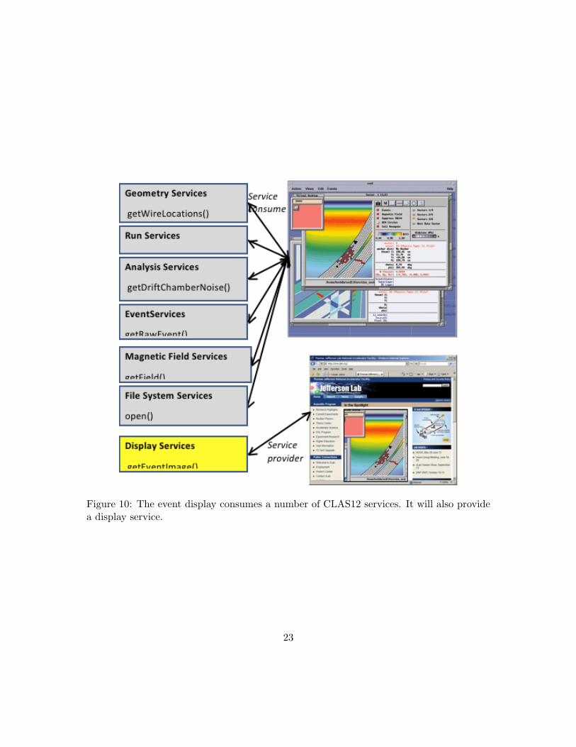
Figure 10: The event display consumes a number of CLAS12 services. It will also providea display service.

23

In this scheme, no recompilation or restart of the event display is required. The devel-oper extending the event display creates the class, drops it into the path, and the class willbe automatically plugged into the application. If a particular plug-in proves of general use,it can be placed in the path of the shared event display (e.g., a run in the counting house)so that all users can access it. On the other hand a class file that posseses undersirable orbuggy features can simply be deleted. Adding and removing features will occur with nochange to the code or recompilation of the base event display.

2.5.3 Data and Algorithm Services

The CLAS12 software design separates data and algorithm services. An algorithm service,in general, will accept and process an output data object from a data service and will thenproduce a new data object.

Data objects are resident on the disk, whereas data services manipulate the data objectsin memory. The algorithm services should be independent of the technology used for dataobject persistency. This will allow the future replacement of persistency technology withoutaffecting the user-produced algorithm services. The separation of persistent and transientdata services is aimed at achieving a higher level of optimization by targeting inherentlydifferent optimization criteria for persistent and transient data storages. For example, theoptimization should target I/O performance, data size, avoid multiple I/O requests, etc.,for data objects on the disk, and execution performance, API and usage simplicity, etc.,for transient data in memory.

We foresee three major categories of data objects:

• Event data, such as raw, simulated, or reconstructed data.

• Detector data, describing a detector apparatus needed to interpret the event data.Examples of detector data are geometry, calibration, alignment, and slow controldata.

• Statistical data, such as histograms, and n-tuples.

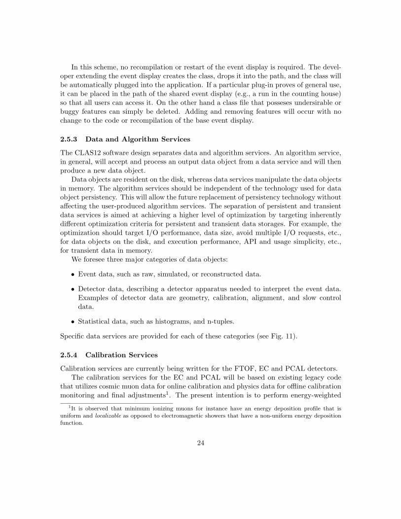
Specific data services are provided for each of these categories (see Fig. 11).

2.5.4 Calibration Services

Calibration services are currently being written for the FTOF, EC and PCAL detectors.The calibration services for the EC and PCAL will be based on existing legacy code

that utilizes cosmic muon data for online calibration and physics data for offline calibrationmonitoring and final adjustments1. The present intention is to perform energy-weighted

1It is observed that minimum ionizing muons for instance have an energy deposition profile that isuniform and localizable as opposed to electromagnetic showers that have a non-uniform energy depositionfunction.

24

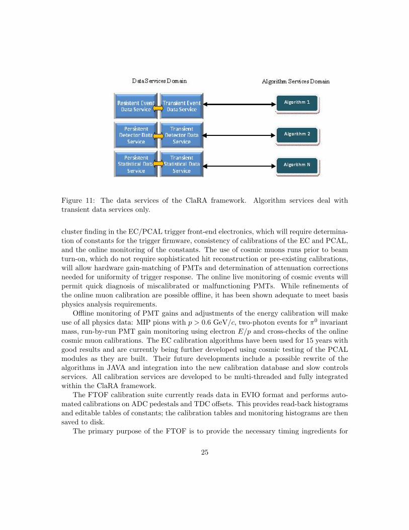
Figure 11: The data services of the ClaRA framework. Algorithm services deal withtransient data services only.

cluster finding in the EC/PCAL trigger front-end electronics, which will require determina-tion of constants for the trigger firmware, consistency of calibrations of the EC and PCAL,and the online monitoring of the constants. The use of cosmic muons runs prior to beamturn-on, which do not require sophisticated hit reconstruction or pre-existing calibrations,will allow hardware gain-matching of PMTs and determination of attenuation correctionsneeded for uniformity of trigger response. The online live monitoring of cosmic events willpermit quick diagnosis of miscalibrated or malfunctioning PMTs. While refinements ofthe online muon calibration are possible offline, it has been shown adequate to meet basisphysics analysis requirements.

Offline monitoring of PMT gains and adjustments of the energy calibration will makeuse of all physics data: MIP pions with p > 0.6 GeV/c, two-photon events for π0 invariantmass, run-by-run PMT gain monitoring using electron E/p and cross-checks of the onlinecosmic muon calibrations. The EC calibration algorithms have been used for 15 years withgood results and are currently being further developed using cosmic testing of the PCALmodules as they are built. Their future developments include a possible rewrite of thealgorithms in JAVA and integration into the new calibration database and slow controlsservices. All calibration services are developed to be multi-threaded and fully integratedwithin the ClaRA framework.

The FTOF calibration suite currently reads data in EVIO format and performs auto-mated calibrations on ADC pedestals and TDC offsets. This provides read-back histogramsand editable tables of constants; the calibration tables and monitoring histograms are thensaved to disk.

The primary purpose of the FTOF is to provide the necessary timing ingredients for

25

particle identification in the forward detector. The raw output data provided by the FTOFwill be recorded as channels from ADC and TDC for PMTs attached to the scintillatorbars. This means that before basic particle identification can be achieved, an intermediatebank of timing information must be combined with tracking information and this timingbank must provide the time of particle interaction at the paddle along with the paddleID/sector. The time of particle interaction at the paddle is calculated simply by takingthe average of the times at the PMTs, adjusted for signal propagation time through thescintillator material. The coupling of a scintillator paddle hit and the corresponding trackthat produced the hit is achieved by “swimming” the track (through a tracking service)to an FTOF scintillator bar identified through the CLAS12 geometry database. Thisintermediate FTOF timing bank is already defined and in use in the Service OrientedTracking (SOT) package as well as the simulation package GEMC.

The secondary purpose of the FTOF is to provide energy deposition information cal-culated from FTOF ADC signals. This particular conversion has yet to be written forCLAS12 specifically, but will follow the standard procedure that was used in CLAS. (Infact, the panel-1a scintillator bars will be salvaged directly from the CLAS TOF detector).It should be noted that the expected energy deposition for a track interacting with anFTOF scintillator bar is currently simulated in GEMC.

The CLAS12 calibration suite is a JAVA-based calibration program that is being writtenas a platform for calibrating the many sub-systems of CLAS12. The design goals are toproduce an agile and modular software system that is fully ClaRA integrated and bothuser and programmer friendly. These goals reflect the clear advantages to future users byhaving a single unified and well maintained program for calibration of all sub-systems, asopposed to the common and unfortunate practice of many different subsystem calibrationprograms being written by a variety of authors in different software languages and thenoften being left unmaintained with the software source hard to find. The program structurehas been kept as simple and lightweight as possible: An orchestrator service acts as a bridgebetween the main GUI and the calibration parent-containers. The parent-containers aremodular groups of calibration services that can be written and plugged directly into theorchestrator with relative ease and minimal changes to the orchestrator or GUI code.

The Calibration Suite accepts EVIO input through the JEvio reader service. Thesuite can be run “offline”, analyzing a predetermined data set, or it can be run “online”continuously accepting data and analyzing it when the user requests. The GUI provides ahistogram readout specific for each calibration type which allows the user to see the qualityof the performed calibrations. To display histograms, our program uses the histogramlibraries from AIDA’s freeHEP project, a JAVA-based and open sourced high energy physicstoolset maintained at SLAC. The output from the calibration routines is also displayed inan in-GUI table which allows the user to inspect and alter the calibration results. The usercan then push the results to disk in an ASCII format file, or send the results directly to acalibration database through the CLAS12 database service.

The first set of calibration algorithms has been implemented for the FTOF, allowing

26

the Calibration Suite to be bug-tested successfully using real CLAS data. The currentgoal for the Calibration Suite is to have complete integration into the ClaRA softwareframework. Version 1.0 (non-ClaRA) is now frozen while the ClaRA-ready Version 2.0 isdeveloped. A set of tools is also being developed to help assist the user in flagging andmanaging problematic calibration results.

27

2.5.5 The Magnetic Field Service

The magnetic field service is implemented in C++. It makes extensive use of the standardlibrary’s map construct. The entire field map is divided into individual maps correspondingto CLAS12 magnets, which comprise the solenoid and main torus. Each of these mapsinherit all capabilities of std::map. In addition, it has methods to get the magnetic fieldat a certain point, check for consistency within the map, and interpolate values inside thedefined grid spacing.

Each map is tailored to the field it holds. For instance, the main torus is defined incylindrical coordinates, with φ ∈ [0, π6 ]. The class holding the main torus map has analgorithm to calculate the field at any point φ ∈ [0, 2π]. However, this is only good forideal fields. For measured fields, the class can be easily extended to handle a case where thefield is known precisely in the entire region. Furthermore, the dimensions and coordinatesof the map’s position and field need not be same. Inside the solenoid field for instance, theposition is stored in (r, φ) while the magnetic field is stored in (x, y, z).

A separate mother class is responsible for loading in and storing the maps from adatabase or file. This class is aware of the volumes of the individual maps and sums thefields where appropriate.

The final layer on this system is the magnetic field service. This is where the motherclass is initialized and held in memory. Several mother classes can be held; i.e. one for theideal fields, one for the measured fields, and one mix of these two. The service registersitself with the ClaRA system and can provide the various field maps in several formatsdepending on the consumer’s preference. As an example, the service can be polled for anentire map or for an individual position.

28

2.6 The CLAS12 Calibration Constants Database

The normal operating procedure for CLAS12 experiments will be a series of short “runs”which will contain data where the configuration is reasonably constant throughout. Forreconstruction and simulation purposes, there will be several sets of constants kept ona run-by-run basis including the geometry and calibration parameters. To this end, adatabase design was created for the GlueX experiment in Hall D (called “CCDB”) and aversion was implemented for CLAS12. This database is intended to store all constants forgeometry and calibration, and possibly the magnetic field maps as well.

Each set of constants is identified by the combination of run number, variation andtime. The variation is a string name or tag to allow several versions of the same constantsto exists for the same run. The time in this case is the time the constants were added tothe database. A running history of changes made to the database is kept and nothing isever deleted. Also, one could substitute the time the data was taken for run number.

Within the ClaRA framework, the CCDB software comes with an interface in C++,JAVA and Python. Constants are obtained by contacting the appropriate service, ei-ther geometry or calibration. The geometry service provides the sets of parameters thatare needed by the simulation (GEMC), track reconstruction (SOT) or other calibrationservices. These parameters are all derived from a unique set of detector-specific “core”numbers. The calibration service is similar, though generally no intermediate calculationsare needed and it acts as a simple interface to the numbers in the database.

29

3 Simulation

3.1 Introduction

A parametric Monte Carlo and a GEANT3-based model of CLAS12, described below, weredeveloped in order to validate design decisions for the upgraded detector. At the same timewe started to build a modern simulation package able to support the engineering projectand meant to be used for the whole lifetime of the CLAS12 program. The result of thiseffort is an entirely new object-oriented design C++ framework called GEMC.

3.1.1 Parametric Monte Carlo

One of the fundamental algorithmic challenges in the design of CLAS12 is the problem oftrack reconstruction in a non-uniform magnetic field. Not only does the torus producean inhomogeneous field in the tracking volume, but charged particles emerging from thesolenoid must be tracked as they traverse the fringe field of that magnet. Since no analyticform for the particle trajectories exist, they must be calculated by ”swimming” the particlesnumerically through a map of the magnetic field. Track fitting then becomes very expensivein terms of CPU time. One way to finesse the problem is to linearize it by parameterizingthe trajectory as small deviations from a reference trajectory. The reference trajectory mustcome from a “swim”, but subsequent “trial” trajectories, with different starting parameters(momentum, direction), can be computed by a simple matrix inversion. Position resolutionis put in at a set of idealized detector planes. It is also possible to incorporate multipleCoulomb scattering in this model. This technique has already been used to estimatemomentum resolution for CLAS12. Results appear in other sections of this document. Themethod cannot give information on some things, such as the effect of accidentals, trackreconstruction efficiency or confusion due to overlapping tracks.

3.1.2 CLAS Software with CLAS12 Geometry

The current CLAS system consists of over a half a million lines of FORTRAN, C and C++code contained in about 2,500 source code files. It represents a large investment by theCLAS collaboration over many years. CLAS, with its toroidal magnetic field also presentsthe difficulty of tracking in a non-homogeneous field and that problem has been solvedin this body of code. Recently, the geometry of crucial detector elements was changedto reflect the CLAS12 design, both in simulation and in reconstruction. The resultingsystem can now do a full GEANT3-based simulation and reconstruction of CLAS12 events,in particular charged particle tracking in the forward drift chambers. Studies using thissystem have been carried out to verify momentum resolution results from the parametricMonte Carlo and to estimate the effect of accidental Møller scattering background on trackreconstruction. More of the details of the detector subsystems and beam line components

30

of the upgraded configuration are being added to extend the range of these and similarstudies.

3.2 GEANT4 Monte Carlo: GEMC

GEMC is a software framework that interfaces with the GEANT4 libraries. It is driven bytwo design principles:

1. Use object oriented design that includes the C++ Standard Template Library. TheGEANT4 solid, logical physical volumes, magnetic fields, sensitivities, etc., are ab-stracted into general classes that can be built from the database of user choice. Forexample, one can use MySQL, GDML or ClaRA to define the geometry.

2. All simulation parameters must be stored in a database external to the code. In otherwords, there are no hardcoded numbers in GEMC. In fact GEMC is agnostic on thedetector: choosing what configuration to use is a matter of choosing what databaseto use, a choice that can be done trivially at run time.

3.2.1 Main GEMC Features

• The users do not need to know the C++ programming language or the GEANT4interface to build detectors. A simple API takes care of the database I/O. This allowsusers to concentrate on making the geometry as realistic as possible.

• Upon database upload (which is an instantaneous MySQL table upload) the geometryis available to all GEMC users - literally across the globe - without having to recompilethe code or even download files.

• Many additional parameters are selectable at run time: displacements, step size,magnetic field scaling, physics list, beam luminosity etc. This is done by eithercommand-line options or a configuration file called “gcard.”

• Rigorous object oriented implementation allows code flexibility and painless, simpledebugging.

3.2.2 GEMC Detector Geometry

The GEANT4 volumes are defined as follows:

• Shapes, dimensions, boolean operations of shapes.

• Material, magnetic field, visual attributes, identity, sensitivity and hit process.

• Placement(s) in space: position, rotation, copy number.

31

These parameters are stored in MySQL tables, one table per detector (i.e. HTCC, EC,DC, etc). Below is an example of the API that loads the parameters into the database:

for(my $n=1; $n<=$NUM_BARS; $n++)

{

# element name, mother, description

$detector{"name"} = "CTOF_Paddle_$pnumber";

$detector{"mother"} = "CTOF" ;

$detector{"description"} = "Central TOF Scintillator $n";

# positioning, rotation, color

$detector{"pos"} = "$x*cm $y*cm $z*cm";

$detector{"rotation"} = "90*deg $theta2*deg 0*deg";

$detector{"color"} = "66bbff";

# Solid type, dimension, materials, style

$detector{"type"} = "Trd";

$detector{"dimensions"} = "$dx1*cm $dx2*cm $dy*cm $dy*cm $dz*cm";

$detector{"material"} = "Scintillator";

$detector{"style"} = 1;

# Magnetic Field

$detector{"mfield"} = "clas12-solenoid";

# Sensitivity: This will associate the volume to the Sensitive Detector

$detector{"sensitivity"} = "CTOF";

# Hit Process: This will associate the volume to the Hit Process routine

$detector{"hit_type"} = "CTOF";

}

At run time, GEMC reads the gcard, an XML file that specifies which detector toinclude in the simulation, including possible tilts and displacements from the original po-sitions. An example of gcard syntax is given below:

<sqltable name="LH2target"/> Includes the Liquid Hidrogen Target

<sqltable name="BST"/> Includes the Barrel Silicon Vertex Tracker

<sqltable name="FST"/> Includes the Forward Silicon Vertex Tracker

<sqltable name="CTOF"/> Includes the Central TOF

<sqltable name="beamline"/> Includes the beamline

<sqltable name="DC"/> Includes the Drift Chambers

<detector name="BST">

<position x="0*cm" y="0.1*cm" z="0*cm" /> Displaces the BST by 1 mm in the Y axis

<rotation x="1*deg" y="0*deg" z="0*deg"/> Tilts the BST by 1 degree around the X axis

</detector>

32

3.2.3 CLAS12 Geometry Implementation

Particular attention is paid in implementing the geometry details of each detector withadequate accuracy. In Fig. 12 the SVT GEMC representation is shown, while in Fig. 13 isshown the GEMC implementation of the various central detectors. A multiple track eventin the central and forward part of CLAS12 can be seen in Fig. 14.

Figure 12: The Silicon Vertex Tracker in GEANT4. Upper left: the GEMC BST. Upperright: the CAD model. Lower Left: the complete GEMC implementation of the BST+FST.Lower right: an FST module. All components (including supports, wirebonds and chips)and dimensions in GEMC reproduce exactly the design.

33

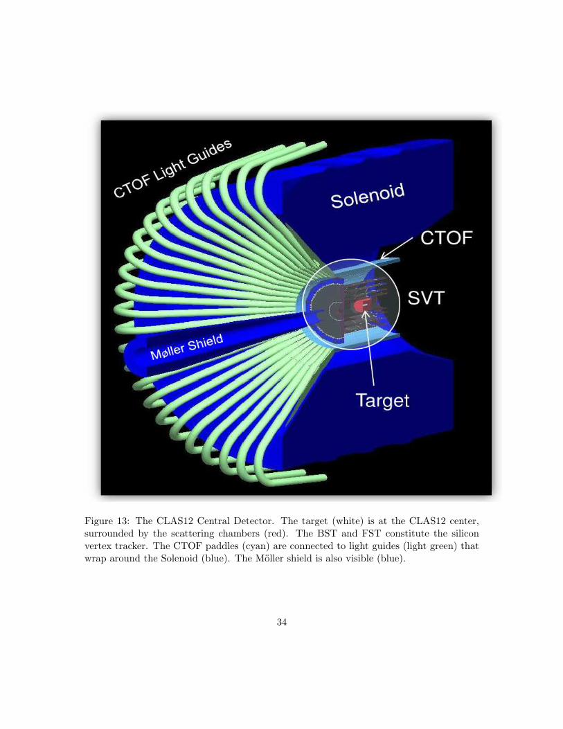
Figure 13: The CLAS12 Central Detector. The target (white) is at the CLAS12 center,surrounded by the scattering chambers (red). The BST and FST constitute the siliconvertex tracker. The CTOF paddles (cyan) are connected to light guides (light green) thatwrap around the Solenoid (blue). The Moller shield is also visible (blue).

34

DC  

LTCC  

FTOF  PCAL  

EC  

HTCC  Central  Detector  BST,  BMT,  FMT,    CTOF,  CND  

Figure 14: The CLAS12 central and forward detectors. In the forward part: the HTCC,3 regions of drift chambers (DC), the LTCC, three panels of time-of-flight and the twoelectro-magnetic calorimeters PCAL and EC. Two simulated tracks produced hits (in red)in the various detector. Photons are the blue straight tracks.

35

3.2.4 Primary Generator

In GEMC there are two ways to define the primary event.

1. GEMC internal generator (command line or gcard): with this method the userdefines the primary particle type, momentum range, vertex range. Example:

BEAM_P="proton, 0.8*GeV, 80*deg, 10*deg" (particle type, momentum, theta and phi)

SPREAD_P="0.2*GeV, 40*deg, 40*deg" (momentum, theta, phi ranges)

BEAM_V="(0.0, 0.0, -10.0)cm" (x,y,z) of the primary vertex

SPREAD_V="(0.1, 2.5)cm" (z, radius ranges) i=for the primary vertex

results in:

Primary Particle: Proton

momentum: 800 +- 200 MeV

theta: 80 +- 40 deg

Phi: 10 +- 40 deg

Vertex: ( +- 1 mm , +- 1mm +- 2.5cm)

2. external input file: with this method the user defines (command line or gcard)the format of the input file and the file name. Example:

INPUT_GEN_FILE="LUND, dvcs.dat" (LUND file format, filename: dvcs.dat)

The various file formats are registered in GEMC by a factory method that allows theuser to derive new formats from the GEMC C++ pure virtual methods defined for theinput and to choose the desired format at run-time.

3.2.5 Beam(s) Generator

In addition to the primary particles, two additional luminosity beams can be defined to addrealistic background to the simulation in the form of N beam particles per event. The userdefines (command line or gcard) the beam particle type, the number of beam particles perevent and the time structure of the beam. Example:

LUMI_P="e-, 11*GeV, 0, 0" Beam Particles: 11 GeV e- along z-axis

LUMI_V="(0, 0, -10)cm" Beam vertex is at z=-10 cm

LUMI_EVENT="60000, 124*ns, 2*ns" 60,000 particles per event, spread in 124 ns, 2ns per bunch

36

3.2.6 Hit Definition

The GEMC hit definition is illustrated in Fig. 15. A Time Window (TW) is associated witheach sensitive detector. In the same detector element, track signals within the TW formone hit, while tracks separated in time by more than the TW will result in multiple hits.

An energy sharing mechanism is in place as well. For each sensitive detector elementusers can decide how much of the energy deposited will be detected in that element. Userscan also decide whether a sensitive element triggers other sensitive elements even if theyare not directly touched by a track, and how much energy is shared between the elements.A good example of this is the charge sharing mechanism in strips in a silicon detector.

Figure 15: Hit definition illustration: In the picture two different detector elements areshown in different colors (red and yellos). All tracks within the same TW and the samecell constitute one hit for that cell. If any track has enough time separation from an existinghit, it will form another, separate hit.

37

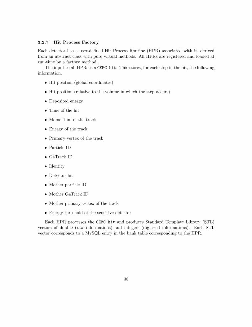
3.2.7 Hit Process Factory

Each detector has a user-defined Hit Process Routine (HPR) associated with it, derivedfrom an abstract class with pure virtual methods. All HPRs are registered and loaded atrun-time by a factory method.

The input to all HPRs is a GEMC hit. This stores, for each step in the hit, the followinginformation:

• Hit position (global coordinates)

• Hit position (relative to the volume in which the step occurs)

• Deposited energy

• Time of the hit

• Momentum of the track

• Energy of the track

• Primary vertex of the track

• Particle ID

• G4Track ID

• Identity

• Detector hit

• Mother particle ID

• Mother G4Track ID

• Mother primary vertex of the track

• Energy threshold of the sensitive detector

Each HPR processes the GEMC hit and produces Standard Template Library (STL)vectors of double (raw informations) and integers (digitized informations). Each STLvector corresponds to a MySQL entry in the bank table corresponding to the HPR.

38

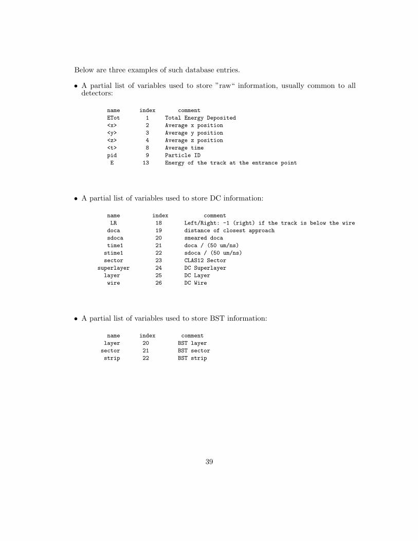
Below are three examples of such database entries.

• A partial list of variables used to store ”raw“ information, usually common to alldetectors:

name index comment

ETot 1 Total Energy Deposited

<x> 2 Average x position

<y> 3 Average y position

<z> 4 Average z position

<t> 8 Average time

pid 9 Particle ID

E 13 Energy of the track at the entrance point

• A partial list of variables used to store DC information:

name index comment

LR 18 Left/Right: -1 (right) if the track is below the wire

doca 19 distance of closest approach

sdoca 20 smeared doca

time1 21 doca / (50 um/ns)

stime1 22 sdoca / (50 um/ns)

sector 23 CLAS12 Sector

superlayer 24 DC Superlayer

layer 25 DC Layer

wire 26 DC Wire

• A partial list of variables used to store BST information:

name index comment

layer 20 BST layer

sector 21 BST sector

strip 22 BST strip

39

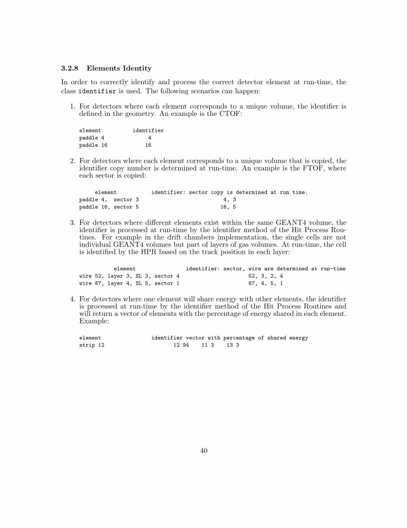
3.2.8 Elements Identity

In order to correctly identify and process the correct detector element at run-time, theclass identifier is used. The following scenarios can happen:

1. For detectors where each element corresponds to a unique volume, the identifier isdefined in the geometry. An example is the CTOF:

element identifier

paddle 4 4

paddle 16 16

2. For detectors where each element corresponds to a unique volume that is copied, theidentifier copy number is determined at run-time. An example is the FTOF, whereeach sector is copied:

element identifier: sector copy is determined at run time.

paddle 4, sector 3 4, 3

paddle 16, sector 5 16, 5

3. For detectors where different elements exist within the same GEANT4 volume, theidentifier is processed at run-time by the identifier method of the Hit Process Rou-tines. For example in the drift chambers implementation, the single cells are notindividual GEANT4 volumes but part of layers of gas volumes. At run-time, the cellis identified by the HPR based on the track position in each layer:

element identifier: sector, wire are determined at run-time

wire 52, layer 3, SL 2, sector 4 52, 3, 2, 4

wire 87, layer 4, SL 5, sector 1 87, 4, 5, 1

4. For detectors where one element will share energy with other elements, the identifieris processed at run-time by the identifier method of the Hit Process Routines andwill return a vector of elements with the percentage of energy shared in each element.Example:

element identifier vector with percentage of shared energy

strip 12 12 94 11 3 13 3

40

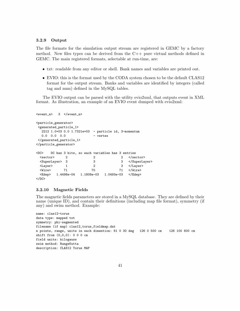
3.2.9 Output

The file formats for the simulation output stream are registered in GEMC by a factorymethod. New files types can be derived from the C++ pure virtual methods defined inGEMC. The main registered formats, selectable at run-time, are:

• txt: readable from any editor or shell. Bank names and variables are printed out.

• EVIO: this is the format used by the CODA system chosen to be the default CLAS12format for the output stream. Banks and variables are identified by integers (calledtag and num) defined in the MySQL tables.

The EVIO output can be parsed with the utility evio2xml, that outputs event in XMLformat. As illustration, an example of an EVIO event dumped with evio2xml:

<event_n> 3 </event_n>

<particle_generator>

<generated_particle_1>

2212 1.0+03 0.0 1.7321e+03 - particle id, 3-momentum

0.0 0.0 0.0 - vertex

</generated_particle_1>

</particle_generator>

<DC> DC has 3 hits, so each variables has 3 entries

<sector> 2 2 2 </sector>

<SuperLayer> 3 3 3 </SuperLayer>

<Layer> 1 2 3 </Layer>

<Wire> 71 70 71 </Wire>

<Edep> 1.4498e-04 1.1808e-03 1.0493e-03 </Edep>

</DC>

3.2.10 Magnetic Fields

The magnetic fields parameters are stored in a MySQL database. They are defined by theirname (unique ID), and contain their definitions (including map file format), symmetry (ifany) and swim method. Example:

name: clas12-torus

data type: mapped txt

symmetry: phi-segmented

filename (if map) clas12_torus_fieldmap.dat

n points, range, units in each dimention: 61 0 30 deg 126 0 500 cm 126 100 600 cm

shift from (0,0,0): 0 0 0 cm

field units: kilogauss

swim method: RungeKutta

description: CLAS12 Torus MAP

41

3.2.11 Parameters Factory

In order to avoid hardcoded numbers in the various software components (simulation,reconstruction, event display, analysis, etc) some “mother numbers” parameters are storedin a MySQL database. These parameters can be accessed by the GEMC geometry API tobuild the GEANT4 volumes via hash map “parameters”:

my $NUM_BARS = $parameters{"ctof_number_of_bars"};

They can also be accessed by the hit-process routines to determine the identifiers and toperform the digitization via an STL map <string, double> “gpars”:

double ec_tdc_time_to_channel = gpars["EC/ec_tdc_time_to_channel"];

3.2.12 Material Factory

The GEANT4 materials definitions, including optical properties, have been abstracted toa material factory. At the command line users can decide to load the materials definitionsfrom the traditional GEANT4 C++ implementation or from a MySQL database. A thirdoption will allow for GDML definitions. Example of MySQL definition:

BusCable | 1200 | 2 | G4_Cu 24 G4_POLYETHYLENE 76

defines the material BusCable with density 1.2 g/cm3, composed of 2 materials: copper(24%) and polyethylene (76%).

3.2.13 Geometry Factory

The current implementation of GEMC builds the GEANT4 solids, logical and physicalvolumes, and sensitive detectors from a MySQL database. The “detector” class will beabstracted to a factory to expand its input to:

• Traditional C++ GEANT4 detector construction

• MySQL DB (current implementation)

• ClaRA: a service will provide detector constructions

• GDML Format: a GEANT4 standard XML syntax, extended for sensitivity andoutput format.

• HDDS Format: XML syntax, extended for sensitivity and output format.

42

3.2.14 Results

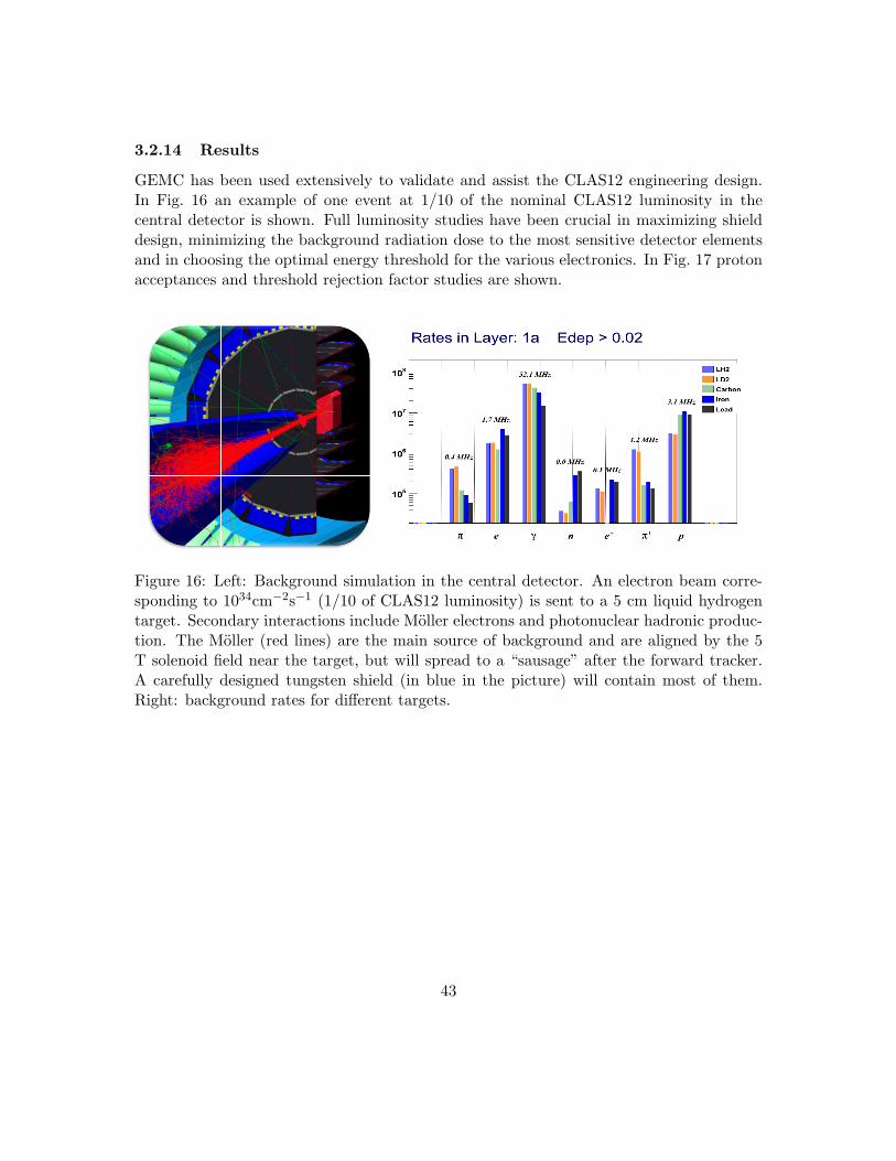
GEMC has been used extensively to validate and assist the CLAS12 engineering design.In Fig. 16 an example of one event at 1/10 of the nominal CLAS12 luminosity in thecentral detector is shown. Full luminosity studies have been crucial in maximizing shielddesign, minimizing the background radiation dose to the most sensitive detector elementsand in choosing the optimal energy threshold for the various electronics. In Fig. 17 protonacceptances and threshold rejection factor studies are shown.

Figure 16: Left: Background simulation in the central detector. An electron beam corre-sponding to 1034cm−2s−1 (1/10 of CLAS12 luminosity) is sent to a 5 cm liquid hydrogentarget. Secondary interactions include Moller electrons and photonuclear hadronic produc-tion. The Moller (red lines) are the main source of background and are aligned by the 5T solenoid field near the target, but will spread to a “sausage” after the forward tracker.A carefully designed tungsten shield (in blue in the picture) will contain most of them.Right: background rates for different targets.

43

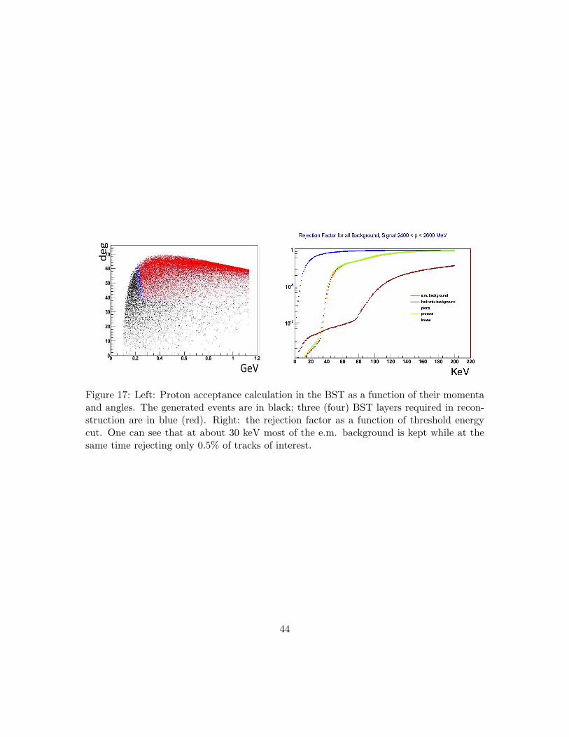
deg  

GeV  

Figure 17: Left: Proton acceptance calculation in the BST as a function of their momentaand angles. The generated events are in black; three (four) BST layers required in recon-struction are in blue (red). Right: the rejection factor as a function of threshold energycut. One can see that at about 30 keV most of the e.m. background is kept while at thesame time rejecting only 0.5% of tracks of interest.

44

3.2.15 Documentation

The main portal to the GEMC documentation is the JLab website:

http://gemc.jlab.org

Various how-tos, tutorials, quick guides, and step by step installation guides can be foundon the website.

The C++ code is documented with doxygen. Classes and methods are defined withinline comments and described in detail. The doxygen documentation is generated nightly.The documentation can be found at:

http://clasweb.jlab.org/clas12/gemc_doxygen

A mailing list

gemc_software@jlab.org

is used as the main channel for news and communication.

3.2.16 Bug Report

GEMC uses Mantis [7], a web-based bug-tracking system. Mantis is written in the PHPscripting language and works with MySQL. Mantis can be browsed from most computersand phones. Bugs are tracked, solutions and debugging are logged, and all the conversationis automatically sent by email to the interested parties. The JLab GEMC Mantis BugReport system can be found at:

https://clasweb.jlab.org/mantisbt

Two screenshots of the website can been seen in Fig. 18.

45

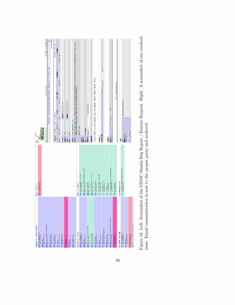
Fig

ure

18:

Lef

t:Sc

reen

shot

ofth

eG

EM

CM

anti

sB

ugR

epor

t/

Feat

ure

Req

uest

.R

ight

:A

scre

ensh

otof

one

reso

lved

issu

e.E

mai

lco

mm

unic

atio

nis

sent

toth

epr

oper

part

yan

dar

chiv

ed.

46

3.2.17 Project Management, Code Distribution and Validation

The software is released on the subversion repository, and it is maintained and tested acrossseveral platforms:

• Darwin macosx 10.7 i386 gcc 4.2.1

• Darwin macosx 10.6 x86 64 gcc 4.2.1

• Darwin macosx 10.7 x86 64 gcc 4.2.1

• Linux CentOS 5.3 i686 gcc 4.1.2

• Linux CentOS 5.3 x86 64 gcc 4.1.2

• Linux RHEL5 i686 gcc 4.1.2

• Linux RHEL6 i686 gcc 4.4.6

• Linux Fedora15 x86 64-gcc4.6

At JLab, GEMC and its dependencies (CLHEP, XERCESC, QT, GEANT4, MySQL) areinstalled and available on the CUE machines (RHEL 5 and 6, CentOS 5) and on the JLabfarm (CeontOS 5). JLab users have been using these distributions since 2008.

M. Ungaro, the author of the code, supervises all aspects of development and has inplace code validation and testing. Cron jobs runs periodically (from as often as 15 minutesto daily) to check the geometry, parameters and material databases, code compilation, etc.For example, if a change is introduced that will cause compilation errors for a particularplatform, his pager will alarm. This system will be expanded in the summer of 2012.

Physics events labelled by the GEMC revision are kept on JLab disks. Scripts that testsignificant quantities (number of particles and hits on specific detectors) will run nightlyas a code quality check.

3.2.18 Project Timeline

The project timeline uses the Omniplan software. Resources are allocated and projects areassigned with duration time. The timeline can be found on the GEMC webpage as a PDFgant chart or a HTML web page:

https://gemc.jlab.org/work/GEMC_Timeline (HTML)

https://gemc.jlab.org/work/GEMC_Timeline.pdf (PDF)

The timeline includes resources management.

47

4 Event Reconstruction

The event reconstruction software has been designed and developed within the ClaRAframework. The reconstruction program must reconstruct, on an event-by-event basis, theraw data coming from either simulation or the detectors to provide physics analysis outputsuch as track parameters and particle identification.

4.1 Tracking

Charged particle tracking is separated into the reconstruction of tracks in the central(“Barrel” Silicon and Micromegas Trackers) and forward (Forward Micromegas Trackerand Drift Chambers) detectors. The forward region covers the angular range from 5◦ to40◦, while the central detector covers approximately 40◦ to 135◦. In the central region a5 T solenoidal magnetic field bends charged tracks into helices, while forward-going tracksare bent by a ∼ 2 T toroidal magnetic field.

For both systems, the reconstruction includes hit recognition, pattern recognition andtrack fitting algorithms. Hit objects, corresponding to the passage of a particle througha particular detector component, involve a combination of an electronic signal and thedetector sub-system geometry. These objects are then manipulated to form the input tothe pattern recognition algorithms. Hit recognition involves clustering of hits and the de-termination of the spatial coordinates and corresponding uncertainties for hits and clustersof hits. At the pattern recognition stage, hits that are consistent with belonging to a tra-jectory (i.e. track) are identified. This set of hits is then fit to the expected trajectory withtheir uncertainties, incorporating the knowledge of the detector material and the detailedfield map.

For central tracking, hit recognition first consists of the determination of the intersectionof clusters of strips in a double layer of the tracker, when projected into the bottom-mostlayer. This is defined as a 3-dimentional point with uncertainty estimated from the clustererror matrix. Since the layers in a double layer are not on the same plane, the locationof this point is trajectory-dependent (it depends upon the crossing angle of the particlewith the BST tile). Hence an iterative algorithm involving the estimate of the tangentto the track at the intersection plane is implemented in order to improve the hit positionaccuracy. The set of central tracker hits is the input to a Hough Transform algorithm.

The Hough Transform is a powerful pattern recognition tool to select groups of hits andis a proven technique to separate real tracks from background. Groups of points belongingto the same trajectory, such as a helix, correspond to the intersection of the continuousdistributions (e.g. lines) in Hough space that the discrete points in the original space mapinto. The algorithm makes use of an array, called an accumulator, with dimensions equalto the number of parameters in Hough space. The bin sizes in the array are finite intervalsin Hough parameters, which are called accumulator cells. The cell with the highest countcorresponds to the intersection of the lines. The output of the Hough Transform algorithm

48

is a track seed that is the input to a fit.A cylindrical coordinate system is a natural choice for the central tracker, with the z

coordinate along the detector axis. The fit is done to state vectors in the (z, φ, px, py, pz)coordinate system, where z is the coordinate in the direction of the beam axis, φ, is theazimuthal angle (from the origin of the laboratory frame), and px, py, pz are the momentumcomponents in the laboratory frame. Two track fitting algorithms have been developed tofit the set of hits that had been identified as a track candidate at the pattern recognitionstep. A simple helical track fit method based on a least square regression approach isemployed in the current version of SOT. A Kalman Filter has also been implemented.The filter starts from the last available measurement (outermost hit) moving towards thetarget and stopping at the distance of closest approach to the beam axis. The algorithmwas validated from a comparison of its results with estimates analytically derived from theFast Monte Carlo program. Very good agreement was found. The fitting code was alsostudied in high background scenarios and the reconstruction involved a small instance offake tracks. The inclusion of the CTOF in the reconstruction chain is aimed at furtherreducing fake tracks.

Hit recognition for forward tracking is detector-dependent. The Forward Micromegasstrip intersection determination is similar to that used in the central region. The DriftChamber (DC) wire hit information is given by the wire geometrical location and the drifttime to the wire. Track-dependent corrections to the hit, such as left-right ambiguity andtime-walk are performed.

Pattern recognition in the DC involves three consecutive steps. First contiguous hitsin the same superlayer and sector are grouped into a cluster. Clusters consistent with aline are linked into segments. This allows the removal of outliers and yields a solutionto the left-right ambiguity of the corresponding hits. The pruning of hits from a clusterrequires an iterative procedure. At each step of the procedure a fit with a straight line isperformed on the set of hits composing a cluster. The hits on the outer edges of the clusterare removed and the hits for which the left-right ambiguity is solved are kept. At this time,four such iterations are required. As for central tracking, the resulting set of hits are sentto a Kalman filter. In the forward geometry, the measurements are approximately constantin z, which makes a natural choice of parameters: x and y, the coordinates transverse tothe beam axis, tanθx and tanθy, the track slope in the xz and yz planes, respectively, andQ/p, the inverse particle momentum. The components of the state vector in this coordinatesystem are initialized to the last plane of Region 3 and from an estimate of the track anglesjust before and just after the toroidal field. The Kalman filter is run up to the distance ofclosest approach to the beam axis, as for central tracking.

In addtion to track fitting in the DC, track matching with the Forward MicromegasTracker (FMT) is performed. Track finding in the FMT is done by selecting combinations ofstrips producing three almost aligned points in space pointing towards the beam axis. Thetrack candidates from the FMT are then matched with those from the DC by extrapolatingthe output of the Kalman filter on DC candidates to the FMT region and looking for a

49

close FMT candidate. We find that requiring that the distance from the extrapolationto the FMT track be within a 1 cm circle allows for a 98% matching efficiency withoutbackground.

The last task of the tracking program will be a vertex fitting algorithm, thus providingfull event reconstruction. Different outputs (not only the structure, but also the contents)will be produced, depending on the incoming request.

4.2 Time-of-Flight

The Time-of-Flight reconstruction service implemented in SOT extrapolates the DC trackstoward the Forward Time-of-Flight (FTOF) detector and attempts to associate each DCtrack with a hit on the FTOF.

The FTOF is designed to measure the time-of-flight of charged particles emerging in theforward direction. Its design parameters were chosen to allow pions and kaons separationup to 3 GeV, with the most energetic particles produced at small angles. The FTOFsystem is comprised of three sets of TOF counters referred to as panels, in each of the sixsectors. Each panel is composed of an array of scintillators with a PMT on each end. Panel1a and 1b are located at forward angles in the range 5 - 36◦ and panel 2 is at larger anglesfrom 35 to 45◦. A charged particle exiting the DC when passing through the scintillatorionizes the material, thereby producing scintillation light which is subsequently detectedby the PMTs. The resulting electronic outputs give ADC and TDC readouts used in thereconstruction.

The current reconstruction algorithm first searches for FTOF hits associated with eachDC track and calculates the distance from the FTOF to the DC. It finds the distance fromthe scintillator to the reference point in the tangent line to the track (assumed to be at theend of the DC) and associates FTOF hits with such distance less than 2 cm.

The timing information from the associated FTOF hits is used in conjunction with thepath-length and reconstruction momentum from the forward Kalman filter to calculateparticle masses for particle identification.

4.3 Cerenkov Counters

In CLAS12, two sets of threshold, non-imaging Cerenkov counters are used in the for-ward region to aid in charged-particle identification. The low-threshold Cerenkov Counter(LTCC), located between the drift chambers and the time-of-flight scintillators, uses theheavy gas C4F10 (n ∼ 1.0015), with a pion threshold of ∼ 2.5 GeV and a kaon thresholdof ∼ 9 GeV, primarily to reject kaons from pion candidates for momenta above the limitfor time-of-flight based π/K separation. The high-threshold Cerenkov Counter (HTCC),located between the exit of the central solenoid and the drift chambers, uses CO2 gas(n ∼ 1.00045) with a pion threshold of 4.9 GeV, primarily to reject negative pions fromelectron candidates in both the online trigger system and the offline analysis.

50

Number of PMTs hit, 100,000 electrons0 2 4 6

0

20000

40000

nhit

Figure 19: Number of HTCC hits per event in GEANT4 for 100,000 electrons with uni-formly distributed momentum (1 ≤ p (GeV) ≤ 11), polar angle (5 ≤ θ(◦) ≤ 35) andazimuthal angle φ (−π ≤ φ ≤ π).

4.3.1 HTCC

In the HTCC, the Cerenkov emission angle for electrons with β ≈ 1 is 1.7◦. The HTCCoptics design consists of 48 individual mirror segments, arranged in four rings subtendingapproximately equal θ-intervals for 5◦ ≤ θ ≤ 35◦, and 12 half-sectors, each subtending a30◦ interval in φ. The ellipsoidal mirror geometry focuses all the light collected onto asingle PMT, resulting in a one-to-one mapping between a given PMT and the range of θand φ covered by its associated mirror segment. The electron path length in CO2 rangesfrom 1.3-1.8 m depending on θ.

Owing to the small size of the Cerenkov emission cone in the HTCC, resulting from thelow index of refraction of CO2, the most probable electron signal in the HTCC is a singlePMT hit. Figure 19 shows the distribution of the number of PMT hits in the HTCC for100,000 generated electrons with flat distributions in momentum from 1-11 GeV, θ from5-35◦, and φ in 2π. Approximately 55% of electrons cause a single hit in the HTCC, whileanother ∼ 40% of events in which electrons pass near the boundary between two mirrorscause two PMTs to fire. The remaining ∼ 5% of events near the intersection point betweenfour mirrors cause 3 or 4 PMTs to fire.

Reconstruction of electron hits in the HTCC involves grouping hits from adjacent mir-rors into clusters to be associated with a single particle track. The simple clusteringalgorithm consists of the following procedure:

1. Populate a list of hits in the event that are not yet part of a cluster.

2. Within this “unused hits” list, find the hit with the largest amplitude; i.e., the greatest

51

number of photoelectrons, and remove it from the “unused hits” list.

3. Search for nearest-neighbor hits of the maximum in the “unused hits” list. For eachnearest-neighbor hit found, add it to the cluster and remove it from the “unused hits”list.

4. Repeat step 3 for all hits in the current cluster, allowing the cluster to grow in anydirection, until no more unused nearest-neighbor hits exist to be added to the cluster.At this point, all hits directly connected to the maximum will have been added tothe cluster seeded by the maximum.

5. Repeat steps 1-4, always starting with the maximum-amplitude unused hit, until nomore hits can be found with which to seed clusters.

The behavior of the clustering algorithm is controlled by a series of three thresholds anda timing cut. The thresholds specify the minimum number of photoelectrons in a clus-ter, the minimum number of photoelectrons in a hit to be considered a valid maximumaround which to build a cluster, and the minimum number of photoelectrons in a hit to beconsidered a valid hit to add to the cluster. The timing cut specifies the maximum timedifference between hits in a cluster. Time offsets for each of the four θ segments are usedto correct for optical photon path length differences between the different mirrors. Thecentral θ and φ values for each ring/half-sector combination are also specified for roughscattering angle reconstruction, neglecting the effect of the solenoid field on the forwardelectron trajectories.

Figure 20 shows the results of the HTCC clustering algorithm for the same 100,000simulated electrons shown in Fig. 19. Exactly one cluster is found in virtually all events,and the number of hits in the cluster equals the number of hits in the event in the over-whelming majority of events. This indicates that the HTCC reconstruction code worksas intended. Figure 21 shows the number of photoelectrons per cluster in the GEANT4simulation of HTCC and the efficiency for electrons as a function of threshold assumingsingle-photoelectron resolution, showing an efficiency exceeding 99% for thresholds up to16 photoelectrons.

4.3.2 LTCC

Each of the six LTCC sectors is spanned in θ by 18 segments, and in φ by 2 modules.The optics of each θ module was designed to focus the light onto the PMT associated withthat module and located in the region obscured by the torus coils. The trajectory of thelight produced by a typical electron passing through the Cerenkov detector is illustratedin Fig. 22. Since the distance between coils increases approximately linearly with θ, eachof the 18 modules has unique optical design parameters.

In the LTCC reconstruction routines clusters of hits are formed. A LTCC clusteris defined as a set of contiguous hits that are time-consistent and contain a threshold

52

nclust

0 1 2 3 40

50

100

310×nclust

nhit

0 2 4 6

nhitc

lust

0

1

2

3

4

5nhitclust:nhit

Figure 20: Left: number of clusters found per event for the same simulated electron sampleshown in Fig. 19. Right: correlation between the number of hits per cluster and the numberof hits per event. A small fraction of events have more hits per event than hits per cluster,reflecting the small additional backgrounds from δ-rays and optical photons reflected bythe PMT windows (∼ 4% probability) onto the mirrors and back into a different PMT(these “echo” hits are less common and separated in time from the primary electron hitsby an interval much larger than the timing resolution of the PMTs).

Number of photoelectrons in cluster0 50 100

0

2000

4000

6000npeclust[0] {npeclust[0]<=100.}

threshold in p. e. (single-p.e. resolution)0 5 10 15 20

elec

tron

eff

icie

ncy

0.97

0.98

0.99

1.00

Figure 21: Left: Number of photoelectrons per cluster in the HTCC GEANT4 simulation.Right: Efficiency for electrons as a function of threshold in photoelectrons, assuming single-photoelectron resolution, averaged over all p, θ and φ.

53

number of photo-electrons (to be determined based on the PMT quantum efficiency andsimulation studies). Once clusters are determined, a matching algorithm will couple themwith existing tracks, if within certain distance and time parameters. An example is givenin Fig. 22 (right), where the signals in the PMTs are associated with the (electron) trackthat generated the Cerenkov light.

Figure 22: Left: Optical arrangement of one of the 216 optical modules of the CLAS Cerenkov detector showingthe optical and light collection components. Note that the Cerenkov PMTs lie in the region obscured by the magnetcoils. Right: Simulation of electron Cerenkov light and its reflections on the LTCC mirrors.

4.4 Calorimeters

The CLAS12 calorimeters will consist of a pre-shower (PCAL) detector which will be builtand installed in front of the current electromagnetic calorimeter (EC). Simulations indi-cated that the EC alone would not be able to absorb the full energy of the electromagneticshowers produced by electrons and photons with momenta above 5 GeV/c. The PCALwas designed with a fine enough granularity in order to allow the reconstruction of high-energy showering particles and to separate high-energy π0’s from photons. Both the ECand PCAL will have similar geometries with three stereo read-out planes composed ofscintillator layers segmented into strips and sandwiched between lead sheets.

The calorimeter reconstruction package contains classes to represent the structure ofthe calorimeter detectors with sector, layer, view and strip components. At this point theEC reconstruction is fully functional and integrated into the ClaRA framework as a service.

In the EC detector, each sector has four layers, each layer has three views, and each viewhas a list with the strips that were stored in the input file. The EC reconstruction containsseveral packages. The event package contains the classes to store the information generatedby the reconstruction algorithm for the event being reconstructed. The reconstruction

54

package contains the algorithms to find peaks in each view, then hits in each layer, tocorrect the timing and energy of the peaks, and finally to find matches of hits betweenlayers.

The EC reconstruction algorithm is split into three services. The first service fills theinformation of strips using the TDC and ADC data obtained from the input file and thecalibration data. The second service is the main one. It iterates over the layers of thesector to get the peaks from the strips and then the hits from the peaks. The third servicematches the hits between the layers in the sector. Finally, when all the six sectors havebeen evaluated, the orchestrator fill the output file with the calculated values.

In addtion, the EC software contains calibration services which at present get thecalibration constants from the CLAS database.

55

4.5 PID for CLAS12

Particle identification (PID) is the procedure of selecting signal events while rejectingbackground events, and is a key step in the data analysis for essentially all particle physicsexperiments. HEP experiments include various approaches from the Bayesian statisticaland log-likelihood technique [8, 9] to more sophisticated Boosted Decision Trees (BDT)[10] and Artificial Neural Networks (ANN) [11].

The identification of the scattered lepton is crucial in electroproduction experiments.The comprehensive research program of CLAS12 comprises both physics with semi-inclusiveand hard exclusive processes, where identification of hadronic particles is also required. Theidentification of electrons and hadrons at CLAS12 is based on the detector responses ofthe forward (EC) and preshower (PCAL) calorimeters, and the High Threshold CherenkovCounter (HTCC). Hadron identification includes the Low Threshold Cerenkov Counter(LTCC), central (CTOF) and forward (FTOF) time-of-flight counters. Particle identifica-tion at CLAS12 will be accomplished combining the reconstructed vertex, momentum andangles from tracking detector (FST, BST, DC) information with responses of the relevantdetector components (HTCC, LTCC, TOF, PCAL, EC). One possible PID scheme forCLAS12 could be a probability-based procedure, where for each particle type a probabilitythat the measured detector signal was caused by that particle is calculated by comparingthe signal with parent distributions which are the typical responses of the different particletypes in the detector.

4.5.1 Probability Analysis

The probability analysis is based on the extraction of probabilities that a measured detectorresponse E was caused by particles of a certain type, Ai. This conditional probabilityP (Ai|E) is related through Bayes’s theorem to the conditional probability P (E|Ai) that aparticle of a given type Ai causes a detector response E:

P (Ai|E) =P (Ai) · P (E|Ai)∑nk=1 P (Ak) · P (E|Ak)

, (1)

where the sum runs over all particle types Ak and P (Ai) is the probability that the particleof type Ai is present in the detector.

The conditional probability P (E|Ai) for a given detector D is equivalent to the par-ent distribution LiD that depends on the particle type, the detector response E, and themomentum p of the particle:

LiD ≡ LiD(E, p, θ). (2)

The parent distributions are an intrinsic property of a PID detector that can be cal-culated through normalizing the appropriate particle counts as a function of the detectorresponse. Eventually the parent distributions will be extracted from the data collected

56

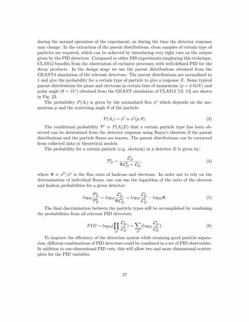
during the normal operation of the experiment, as during the time the detector responsemay change. In the extraction of the parent distributions, clean samples of certain type ofparticles are required, which can be achieved by introducing very tight cuts on the outputgiven by the PID detectors. Compared to other DIS experiments employing this technique,CLAS12 benefits from the observation of exclusive processes with well-defined PID for thedecay products. In the design stage we use the parent distributions obtained from theGEANT4 simulation of the relevant detectors. The parent distributions are normalized to1 and give the probability for a certain type of particle to give a response E. Some typicalparent distributions for pions and electrons in certain bins of momentum (p = 4 GeV) andpolar angle (θ = 15◦) obtained from the GEANT simulation of CLAS12 [12, 13] are shownin Fig. 23.

The probability P (Ai) is given by the normalized flux φi which depends on the mo-mentum p and the scattering angle θ of the particle:

P (Ai) = φi ≡ φi(p, θ). (3)

The conditional probability P i ≡ P (Ai|E) that a certain particle type has been ob-served can be determined from the detector response using Bayes’s theorem if the parentdistributions and the particle fluxes are known. The parent distributions can be extractedfrom collected data or theoretical models.

The probability for a certain particle (e.g. electron) in a detector D is given by:

PeD =LeD

ΦLhD + LeD, (4)

where Φ ≡ φh/φe is the flux ratio of hadrons and electrons. In order not to rely on thedetermination of individual fluxes, one can use the logarithm of the ratio of the electronand hadron probabilities for a given detector:

log10PeDPhD

= log10LeD

ΦLhD= log10

LeDLhD− log10Φ. (5)

The final discrimination between the particle types will be accomplished by combiningthe probabilities from all relevant PID detectors:

PID = log10(∏D

LeDLhD

) =∑D

(log10LeDLhD

). (6)

To improve the efficiency of the detection system while retaining good particle separa-tion, different combinations of PID detectors could be combined in a set of PID observables.In addition to one-dimensional PID cuts, this will allow two and more dimensional scatter-plots for the PID variables.

57

A similar procedure could be used for hadron identification involving the low thresholdCherenkov counter (LTCC) and forward TOF for forward tracks and central TOF for largeangle track identification.

Figure 24 shows (on the left-hand side) the distribution of β as a function of themomentum in the laboratory frame for reconstructed pions, kaons and protons candidates.These events were generated using the GEMC simulation program and reconstructed withSOT with the EC and PID services included in the service chain. Clear bands allowingfor particle identification are visible. On the right-hand side of the figure the invariantmass distributions for the three types of particles reconstructed are shown. The upper plotindicates the clear separation between e− and π− candidates obtained from the EC.

58

10-6

10-5

10-4

10-3

10-2

10-1

0 5 10 15 20 25 30 35 40Nphe

π-

e- π-

e-

EPCAL/P

10-4

10-3

10-2

10-1

1

0 0.2 0.4 0.6 0.8 1 1.2

π-

e-

EEC+PCAL/P

0

0.05

0.1

0.15

0.2

0.25

0 0.2 0.4 0.6 0.8 1 1.2

Figure 23: Parent distributions for π− and electrons for the high threshold Cherenkovcounter (HTCC), the preshower (PCAL) and the sum of the responses of the preshower andthe forward calorimeter (PCAL+EC). The distributions for electrons (pions) correspondto histograms with solid (dashed) lines. In the upper left plot, the dotted-line histogramcorresponds to the distribution of 2 GeV pions.

59

Figure 24: [left] The distribution of β as a function of the momentum in the laboratoryframe for reconstructed pions, kaons and protons candidates. [right] The invariant massdistributions for the three types of particles reconstructed.

60

5 Software Tools

Various object-oriented programs and libraries developed for particle physics data analysisare currently in existence and freely available. ROOT, the C++ program library developedby CERN includes packages for histogramming, curve fitting, matrix algebra, multivari-ate analysis, four-vector operation and various statistical tools used in data analysis. ForPython developement, SciPy [16] is the scientific data analysis system based on NumPy [17]classes. Numpy contains a powerful N -dimensional array object, sophisticated (broadcast-ing) functions, tools for integrating C/C++ and Fortran code, as well as useful linearalgebra, Fourier transform, and random number capabilities. The SciPy library is builtto work with NumPy objects, and provides efficient numerical routines such as numericalintegration and optimization. Together, they run on all popular operating systems, areeasy to install, and are free of charge.

Java-based data analysis systems include JAS (Java Analysis Studio) [18], which iscompliant with AIDA (Abstract Interface for Data Analysis) [19], and jHepWork, whoseframework is based on FreeHep. FreeHEP is an open source Java library designed to makeprogramming applications easier and to encourage the sharing and reuse of Java code inHigh Energy Physics. FreeHEP provides utilities for event display (WIRED), fast detectorsimulation (Lelaps) and HEP software. It also provides an implementation for AIDA. TheColt project is another Open Source set of libraries in Java. This is a partial Java portof CLHEP. CLHEP (Class Library for High Energy Physics) [20] is a C++ library thatprovides utility classes for general numerical programming, vector arithmetic, geometry,pseudorandom number generation, and linear algebra, specifically targeted for high energyphysics simulation and analysis software.

The toolkits listed above are recognized in the High Energy Physics community asexcellent standards which the CLAS12 software group will support. The CLAS12 softwaregroup also maintains a set of general software tools both in Java and C++, and it isanticipated that a set of specific tools will also be developed in the future in Python.The Java package is the so-called jMath package, and includes a wide variety of softwareutilities, ranging from graphic and animation tools, relativistic kinematics, matrix algebra,partial wave analysis, numerical methods, and others. In some cases, similar tools are alsoavailable in C++. In the future, it is anticipated that useful packages in Maple [21] and/orMathematica [22] will become a standard part of the CLAS12 software suite.

The CLAS12 simulation package, GEMC, is based on GEANT4, a toolkit for the sim-ulation of the passage of particles through matter. Geant4 is now a standard not only inthe High Energy community, but wider scientific and industral applications as well.

The CLAS12 collaboration has adopted the Calibration and Conditions database origi-nally developed for the GlueX collaboration at JLab (see section 2.6). The database needsof both CLAS12 and GlueX are so similar, it did not seem prudent to develop an entirelyseparate and independent system. Excellent collaboration between the two experimentshas guaranteed a good product meeting the specific needs of both groups.

61

While a final ’post-processed’ data format has not yet been adopted, there are severalcandidates. EVIO is a data format designed by and maintained by the Jefferson Labo-ratory Data Acquisition Group, and is the data format of the raw data. It may also beutilized as the post-processed data format. In addition, we are evaluating HDF5, originallydeveloped by the HDF Group at the National Center for Supercomputing Applications atthe University of Illinois, which has developed this data format over the past twenty years.The HDF5 serial and parallel I/O library is the result of the collaboration of NCSA withthree DOE laboratories: Lawrence Livermore National Laboratory (LLNL), Sandia Na-tional Laboratory (SNL) and Los Alamos National Laboratory (LANL). HDF5 is a datamodel, library, and file format for storing and managing data. It supports an unlimitedvariety of datatypes, and is designed for flexible and efficient I/O and for high volumeand complex data. HDF5 is portable and is extensible, allowing the evolution of the dataformat. The HDF5 suite includes a versatile data model that can represent very complexdata objects and a wide variety of metadata. It is a portable file format with no limit onthe number or size of data objects in the collection, and also includes a software librarythat runs on a wide range of computational platforms, and implements a high-level APIwith C, C++, Fortran 90, and JAVA interfaces. Integrated performance features allow foraccess time and storage space optimizations.

62

6 Post-Reconstruction Data Access

Due to the distributed nature of the CLAS12 software, a new approach (format) was neededto store physics data. The data formats used by CLAS collaboration lack some key featureswhich we need for distributed multi-process cloud computing.

A new data format based on HDF5 was developed, where the data is stored in anindexed tree for random access, and also the structure of the data is stored in a form of adictionary.

Each data segment that is read from the file comes with a dictionary defining the datastructure. This flexibility allows the services (that process user data) to have no predefineddata structures, but rather to receive the data structure through run-time dictionaries.With this approach several users can simultaneously use services with data sets that havedifferent structures. This format was developed by the Data Mining group at Old DominionUniversity2. The Data Mining group created a framework around HDF5 library thatallows flexible dictionary driven data structures to be effectively exchanged between theservices and the storage.

The Data Mining project makes use of the ClaRA framework. The distributed cloudcomputing environement of ClaRa is well-suited for data mining as well as for CLAS12post-reconstruction data access goals.

The data from the CLAS experiment on nuclear targets is stored on ODU NAS disks.The data is converted from the standard CLAS data format into HDF5 format, and itis indexed by experiment and run conditions. The user can access specific sets of dataspecifying what beam energy, target and beam intensity are required. The ODU computercluster is running several services that provide information on what data is available andwhich services are available to analyze the data. The newly developed framework allowsmultiple processors to cooperate to handle each job, making the data transfer from thedisk the ultimate bottleneck. In the future we plan to distribute the data to several serversat participating universities, which will significantly increase the data analysis.

2The Data Mining project aims to collect the data from multi-hadron runs from the CLAS detector andto develop tools for easy access and analysis for participating universities. This framework could also beextended to include other data sets from Jefferson Lab, which will allow users to analyze the existing datawhile the JLab accelerator is shut down for the upgrade.

63

7 Online Software

During the actual data-taking periods of CLAS12, it is of course expected that therewill be full reconstruction of a significant fraction of the acquired data. Online eventreconstruction allows data quality monitoring and assessment. It also allows the detailedmonitoring of the individual detectors beyond the information given by hardware readoutsby providing various reconstruction outputs such as wire profiles, ADC spectra, etc. Thecapability to study the performance of the CLAS12 detector by examining specific eventsand extracting their physics parameters will require full event reconstruction. In addition,online reconstruction can also act as a Level 3 trigger to filter unwanted events from thedata stream, thus minimizing storage, bandwidth, and other precious resources.

The entire suite of services will be available to the online and data acquisition systems,either directly as network available resources, or as shared code. It is anticipated that amodest cluster of multi-processor, multi-core nodes, of the order of 20 nodes, will be ableto keep up with the data rate, based on current timing studies of SOT (SOT was used toobtain a conservative estimate as the track-reconstruction time dominates the processingtime of an event).

64

8 Code Development and Distribution

8.1 Code Management

For CLAS12, we have elected to use the widely adopted and free (Open Source) “sub-version” revision control system. Subversion is the Open Source software community’sreplacement for cvs. It has many of the same features and employs the same no-lockoutparadigm3 In addition, subversion plugins are available for the popular integrated develop-ment environments, such as the widely used Eclipse [23]. This allows one to check in, checkout, track changes, and merge differences with mouse-clicks in a development environmentrather than through a command line.

In CLAS12, we have decided to implement a three-tiered code distribution system.The first level will give access to the subversion repository. Only developers will accesscode in this manner. The second level will be for code releases, in the form of archives,and intelligent build scripts that do not rely on environment variables. In the CLAS12environment the user will go to a web page and download a specific, tested release. Athird tier of release for limited systems (JLab-supported Linux systems) will be for thedistribution of binaries.

8.2 Code Release

The CLAS12 software release process will be based on the “agile programming ” approach.Part of agile programming is a rapid release schedule. The exact frequency has not yetbeen determined, but the canonical duration is of the order of one month: two weeks ofdevelopment and two weeks of testing and bug fixing. So about every month a new versionof all software will be released, typically with modest changes from the previous release.Functionality is advanced incrementally as opposed to infrequent but massively differentupdates.

8.3 Software Tracking

Complicated software development is aided by requirements, tasks, and bug-tracking. Man-tis [7] is been utilized for bug-tracking. Project management is implemented via Ganttcharts. No release schedule is currently available as there isn’t yet an official release of areconstruction suite.

Ultimately, time development will match the code release cycles. For each cycle, the newtasks and necessary bug fixes will be entered into project management charts. Developers,in communication with the Project Managers, will enter estimates regarding the time it willtake to complete the tasks and fix the bugs. Project managers will evaluate if the estimatedtime fits within the cycle duration and adjust the schedule accordingly by postponing or

3Conflicts are resolved through merging rather than avoided through code locks–the latter is generallyfound to be too draconian and a hindrance to productivity.

65

adding tasks. Developers will keep a log of the time they spend on a specific task or bug fix,which will help them fine-tune their task-specific time estimates. The subversion revisioncontrol system can be set up to require that code checked-in have a comment tying it byID to a task or to a bug.

66

9 Quality Assurance

The Service Oriented Architecture is composed of many integrated services that are looselyconnected. The usual interaction between the consumer of a service and the supplier of theservice is not direct: generally there will be several processes and a network in between.As a result, during an extended development process, many errors can be introduced in thecode, rendering it either unusable or incorrect. Quality assurance of developing projectsthen becomes a major concern.

The standard CLAS12 reconstruction suite of services will be built daily and the re-construction package tested using a set of standard datasets. A reconstruction validationpackage will output a series of indicators of the reconstruction performance and resultconsistency.

The software validation studies will be performed on simulated and real data. MonteCarlo simulations of events produced in fixed target reactions in the CLAS12 detector(see Section 7) will be run through the full reconstruction suite. Detailed checks for dis-crepancies between reconstructed and generated values exceeding the range expected fromresolution effects will be performed using these simulated data. In addition, benchmarkdatasets recorded by the CLAS12 detector will be used to test the reconstruction softwareand track its development.

The reconstruction outputs will be stored in a database and tracked over time to identifychanges in the program performance. In addition, the Subversion code repository (seeSection 8) will allow immediate identification of unanticipated code changes. Subversionalso allows individual code developers to check any version against the standard suite.

67

10 Computing Requirements

In this section we present an estimate of the computing resources required by the CLAScollaboration to acquire, reconstruct, simulate and analyze the CLAS12 data in a timelyfashion. We assume that tasks like reconstruction and simulation will keep pace withthe data acquisition after the start of data taking for CLAS12 in 2015. The computingenterprise for CLAS12 is divided into stages: data acquisition, calibration, reconstruction,simulation, reconstruction studies and physics analysis. The first four stages representthe process of taking the raw data and turning it into 4-momenta and identified particles.The reconstruction studies are needed to optimize the reconstruction of the data and thesimulation, while the physics analysis stage represents a broad range of activities using theresults of the final event sample (measured and simulated).

We now discuss the computing requirements for the data acquisition and focus on thenumber of computing cores, disk space, and tape storage. Table 8 shows the assumptionsthat go into our calculations. Using the data in Table 8 we calculate the data rate, the

Event rate 10 kHz Weeks running 35Event size 10 kBytes 24 hour duty factor 60%

Table 1: Data Acquisition parameters.

number of events collected in a year of running, and the volume of that data.

Data Rate = Event Rate× Event Size = 100 MByte/s (7)

Average 24-hour rate = Data Rate× 24 hour duty factor = 60 MByte/s (8)

Events/year = Event Rate×Weeks Running × 24 hour duty factor (9)= 1.3× 1011 Events/yr

Data Volume/year = Events/year× Event size = 1270 TByte/yr (10)

These results will be used in the calculations below.We next consider the resources we will need to calibrate our data and keep pace with

the incoming data in CLAS12. We have determined the CPU-time to reconstruct an eventfrom previous work with the CLAS12 physics-based simulation GEMC. That result andother assumptions are in Table 9. Calculations of the necessary CPU time in seconds

68

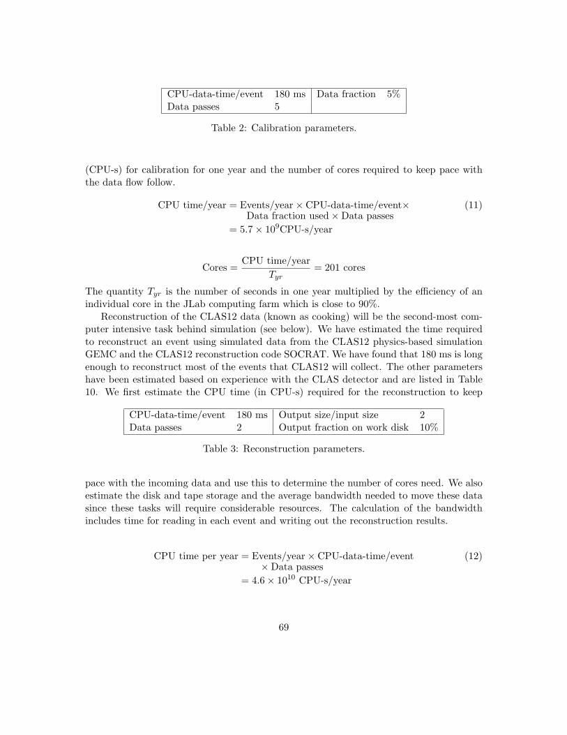
CPU-data-time/event 180 ms Data fraction 5%Data passes 5

Table 2: Calibration parameters.

(CPU-s) for calibration for one year and the number of cores required to keep pace withthe data flow follow.

CPU time/year = Events/year× CPU-data-time/event× (11)Data fraction used×Data passes

= 5.7× 109CPU-s/year

Cores =CPU time/year

Tyr= 201 cores

The quantity Tyr is the number of seconds in one year multiplied by the efficiency of anindividual core in the JLab computing farm which is close to 90%.

Reconstruction of the CLAS12 data (known as cooking) will be the second-most com-puter intensive task behind simulation (see below). We have estimated the time requiredto reconstruct an event using simulated data from the CLAS12 physics-based simulationGEMC and the CLAS12 reconstruction code SOCRAT. We have found that 180 ms is longenough to reconstruct most of the events that CLAS12 will collect. The other parametershave been estimated based on experience with the CLAS detector and are listed in Table10. We first estimate the CPU time (in CPU-s) required for the reconstruction to keep

CPU-data-time/event 180 ms Output size/input size 2Data passes 2 Output fraction on work disk 10%

Table 3: Reconstruction parameters.

pace with the incoming data and use this to determine the number of cores need. We alsoestimate the disk and tape storage and the average bandwidth needed to move these datasince these tasks will require considerable resources. The calculation of the bandwidthincludes time for reading in each event and writing out the reconstruction results.

CPU time per year = Events/year× CPU-data-time/event (12)×Data passes

= 4.6× 1010 CPU-s/year

69

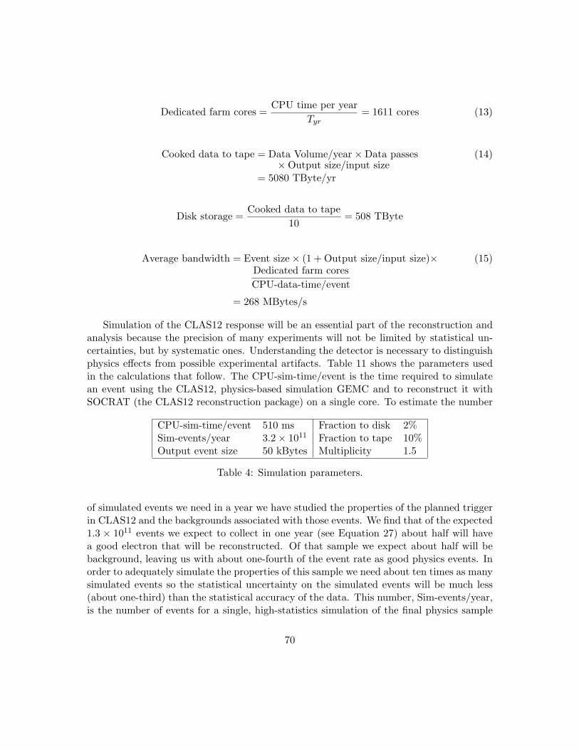
Dedicated farm cores =CPU time per year

Tyr= 1611 cores (13)

Cooked data to tape = Data Volume/year×Data passes (14)×Output size/input size

= 5080 TByte/yr

Disk storage =Cooked data to tape

10= 508 TByte

Average bandwidth = Event size× (1 + Output size/input size)× (15)Dedicated farm coresCPU-data-time/event

= 268 MBytes/s

Simulation of the CLAS12 response will be an essential part of the reconstruction andanalysis because the precision of many experiments will not be limited by statistical un-certainties, but by systematic ones. Understanding the detector is necessary to distinguishphysics effects from possible experimental artifacts. Table 11 shows the parameters usedin the calculations that follow. The CPU-sim-time/event is the time required to simulatean event using the CLAS12, physics-based simulation GEMC and to reconstruct it withSOCRAT (the CLAS12 reconstruction package) on a single core. To estimate the number

CPU-sim-time/event 510 ms Fraction to disk 2%Sim-events/year 3.2× 1011 Fraction to tape 10%Output event size 50 kBytes Multiplicity 1.5

Table 4: Simulation parameters.

of simulated events we need in a year we have studied the properties of the planned triggerin CLAS12 and the backgrounds associated with those events. We find that of the expected1.3 × 1011 events we expect to collect in one year (see Equation 27) about half will havea good electron that will be reconstructed. Of that sample we expect about half will bebackground, leaving us with about one-fourth of the event rate as good physics events. Inorder to adequately simulate the properties of this sample we need about ten times as manysimulated events so the statistical uncertainty on the simulated events will be much less(about one-third) than the statistical accuracy of the data. This number, Sim-events/year,is the number of events for a single, high-statistics simulation of the final physics sample

70

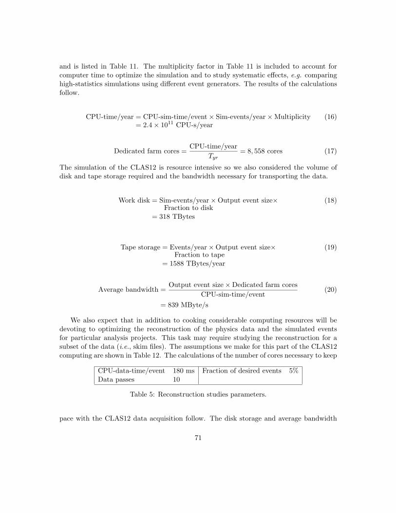
and is listed in Table 11. The multiplicity factor in Table 11 is included to account forcomputer time to optimize the simulation and to study systematic effects, e.g. comparinghigh-statistics simulations using different event generators. The results of the calculationsfollow.

CPU-time/year = CPU-sim-time/event× Sim-events/year×Multiplicity (16)= 2.4× 1011 CPU-s/year

Dedicated farm cores =CPU-time/year

Tyr= 8, 558 cores (17)

The simulation of the CLAS12 is resource intensive so we also considered the volume ofdisk and tape storage required and the bandwidth necessary for transporting the data.

Work disk = Sim-events/year×Output event size× (18)Fraction to disk

= 318 TBytes

Tape storage = Events/year×Output event size× (19)Fraction to tape

= 1588 TBytes/year

Average bandwidth =Output event size×Dedicated farm cores

CPU-sim-time/event(20)

= 839 MByte/s

We also expect that in addition to cooking considerable computing resources will bedevoting to optimizing the reconstruction of the physics data and the simulated eventsfor particular analysis projects. This task may require studying the reconstruction for asubset of the data (i.e., skim files). The assumptions we make for this part of the CLAS12computing are shown in Table 12. The calculations of the number of cores necessary to keep

CPU-data-time/event 180 ms Fraction of desired events 5%Data passes 10

Table 5: Reconstruction studies parameters.

pace with the CLAS12 data acquisition follow. The disk storage and average bandwidth

71

were calculated in the same manner as the previous ones and we found requirements of 508TBytes for disk and 78 MByte/s for bandwidth.

CPU time per year = Fraction desired× (Events/year + Sim-events/year)× (21)Data passes× CPU-data-time/event

= 4.0× 1010 CPU-s/year

Dedicated farm cores =CPU time per year

Tyr= 1410 cores (22)

Once the reconstruction has been optimized for a particular analysis project, we expectthere will be considerable computing resources devoted to analyzing the results. These datawill not require a full reconstruction so the compute time per event will drop considerably,but the full data set will usually be studied. The assumptions we make for this part of theCLAS12 computing enterprise are shown in Table 13. The calculations of the number of

CPU-analysis-time/event 9 ms Fraction of desired events 50%Data passes 10

Table 6: Physics Analysis parameters.

cores necessary to keep pace with the CLAS12 data acquisition follow. The disk storageand average bandwidth were calculated in the same manner as the previous ones and wefound requirements of 889 TBytes for disk and 279 MByte/s for bandwidth.

CPU time per year = Fraction desired× (Events/year + Sim-events/year)×Data passes×(23)

Data passes× CPU-analysis-time/event= 2.0× 1010 CPU-s/year

Dedicated farm cores =CPU time per year

Tyr= 705 cores (24)

To summarize our estimates we present Table 14. It lists the number of cores, disk,and tape storage required for the different stages of the CLAS12 computing enterpriseplus totals for each item. This is our estimate of the computing resources necessary forthe CLAS collaboration to analyze the data from CLAS12 in a timely and productivemanner. Note the number of cores required for simulation is more than the number forreconstruction, post-reconstruction analysis, and physics analysis combined.

72

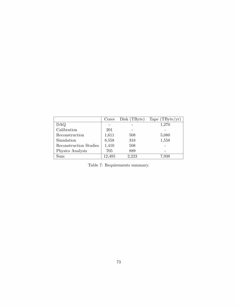
Cores Disk (TByte) Tape (TByte/yr)DAQ - - 1,270Calibration 201 - -Reconstruction 1,611 508 5,080Simulation 8,558 318 1,558Reconstruction Studies 1,410 508 -Physics Analysis 705 889 -Sum 12,485 2,223 7,938

Table 7: Requirements summary.

73

11 Computing Requirements

In this section we present an estimate of the computing resources required by the CLASCollaboration to acquire, reconstruct, simulate and analyze the CLAS12 data in a timelyfashion. We assume that tasks like reconstruction and simulation will keep pace withthe data acquisition after the start of data taking for CLAS12 in 2015. The computingenterprise for CLAS12 is divided into stages: data acquisition, calibration, reconstruction,simulation, reconstruction studies and physics analysis. The first four stages representthe process of taking the raw data and turning it into 4-momenta and identified particles.The reconstruction studies are needed to optimize the reconstruction of the data and thesimulation while the physics analysis stage represents a broad range of activities using theresults of the final event sample (measured and simulated).

We now discuss the computing requirements for the data acquisition and focus on thenumber of computing cores, disk space, and tape storage. Table 8 shows the assumptionsthat go into our calculations. Using the data in Table 8 we calculate the data rate, the

Event rate 10 kHz Weeks running 35Event size 10 kBytes 24 hour duty factor 60%

Table 8: Data Acquisition parameters.

number of events collected in a year of running, and the volume of that data.

Data Rate = Event Rate× Event Size = 100 MByte/s (25)

Average 24-hour rate = Data Rate× 24 hour duty factor = 60 MByte/s (26)

Events/year = Event Rate×Weeks Running × 24 hour duty factor (27)= 1.3× 1011 Events/yr

Data Volume/year = Events/year× Event size = 1270 TByte/yr (28)

These results will be used in the calculations below.We next consider the resources we will need to calibrate our data and keep pace with

the incoming data in CLAS12. We have determined the CPU-time to reconstruct an eventfrom previous work with the CLAS12 physics-based simulation GEMC and the CLAS12reconstruction code SOT. We found that 155 ms is long enough to reconstruct most ofthe events that CLAS12 will collect. That result and other assumptions are in Table 9.Calculations of the necessary CPU time in seconds (CPU-s) for calibration for one year

74

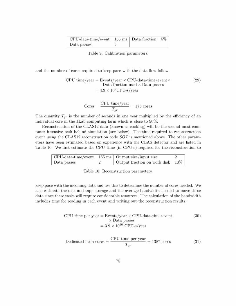
CPU-data-time/event 155 ms Data fraction 5%Data passes 5

Table 9: Calibration parameters.

and the number of cores required to keep pace with the data flow follow.

CPU time/year = Events/year× CPU-data-time/event× (29)Data fraction used×Data passes

= 4.9× 109CPU-s/year

Cores =CPU time/year

Tyr= 173 cores

The quantity Tyr is the number of seconds in one year multiplied by the efficiency of anindividual core in the JLab computing farm which is close to 90%.

Reconstruction of the CLAS12 data (known as cooking) will be the second-most com-puter intensive task behind simulation (see below). The time required to reconstruct anevent using the CLAS12 reconstruction code SOT is mentioned above. The other param-eters have been estimated based on experience with the CLAS detector and are listed inTable 10. We first estimate the CPU time (in CPU-s) required for the reconstruction to

CPU-data-time/event 155 ms Output size/input size 2Data passes 2 Output fraction on work disk 10%

Table 10: Reconstruction parameters.

keep pace with the incoming data and use this to determine the number of cores needed. Wealso estimate the disk and tape storage and the average bandwidth needed to move thesedata since these tasks will require considerable resources. The calculation of the bandwidthincludes time for reading in each event and writing out the reconstruction results.

CPU time per year = Events/year× CPU-data-time/event (30)×Data passes

= 3.9× 1010 CPU-s/year

Dedicated farm cores =CPU time per year

Tyr= 1387 cores (31)

75

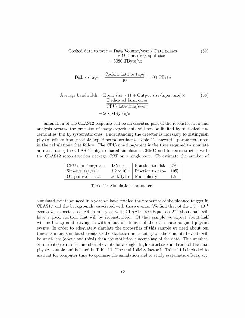
Cooked data to tape = Data Volume/year×Data passes (32)×Output size/input size

= 5080 TByte/yr

Disk storage =Cooked data to tape

10= 508 TByte

Average bandwidth = Event size× (1 + Output size/input size)× (33)Dedicated farm coresCPU-data-time/event

= 268 MBytes/s

Simulation of the CLAS12 response will be an essential part of the reconstruction andanalysis because the precision of many experiments will not be limited by statistical un-certainties, but by systematic ones. Understanding the detector is necessary to distinguishphysics effects from possible experimental artifacts. Table 11 shows the parameters usedin the calculations that follow. The CPU-sim-time/event is the time required to simulatean event using the CLAS12, physics-based simulation GEMC and to reconstruct it withthe CLAS12 reconstruction package SOT on a single core. To estimate the number of

CPU-sim-time/event 485 ms Fraction to disk 2%Sim-events/year 3.2× 1011 Fraction to tape 10%Output event size 50 kBytes Multiplicity 1.5

Table 11: Simulation parameters.

simulated events we need in a year we have studied the properties of the planned trigger inCLAS12 and the backgrounds associated with those events. We find that of the 1.3× 1011

events we expect to collect in one year with CLAS12 (see Equation 27) about half willhave a good electron that will be reconstructed. Of that sample we expect about halfwill be background leaving us with about one-fourth of the event rate as good physicsevents. In order to adequately simulate the properties of this sample we need about tentimes as many simulated events so the statistical uncertainty on the simulated events willbe much less (about one-third) than the statistical uncertainty of the data. This number,Sim-events/year, is the number of events for a single, high-statistics simulation of the finalphysics sample and is listed in Table 11. The multiplicity factor in Table 11 is included toaccount for computer time to optimize the simulation and to study systematic effects, e.g.

76

comparing high-statistics simulations using different event generators. The results of thecalculations follow.

CPU-time/year = CPU-sim-time/event× Sim-events/year×Multiplicity (34)= 2.3× 1011 CPU-s/year

Dedicated farm cores =CPU-time/year

Tyr= 8, 139 cores (35)

The simulation of the CLAS12 is resource intensive so we also considered the volume ofdisk and tape storage required and the bandwidth necessary for transporting the data.

Work disk = Sim-events/year×Output event size× (36)Fraction to disk

= 318 TBytes

Tape storage = Events/year×Output event size× (37)Fraction to tape

= 1, 588 TBytes/year

Average bandwidth =Output event size×Dedicated farm cores

CPU-sim-time/event(38)

= 839 MByte/s

We also expect that in addition to reconstruction and simulation considerable com-puting resources will be devoted to optimizing the reconstruction of the physics data andthe simulated events for particular analysis projects. This task may require studying thereconstruction for a subset of the data (i.e., skim files). The assumptions we make for thispart of the CLAS12 computing are shown in Table 12. The calculations of the number of

CPU-data-time/event 155 ms Fraction of desired events 5%Data passes 10

Table 12: Reconstruction studies parameters.

cores necessary to keep pace with the CLAS12 data acquisition follow. The disk storageand average bandwidth were calculated in the same manner as the previous ones and we

77

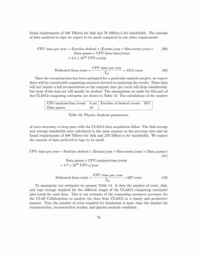
found requirements of 508 TBytes for disk and 78 MByte/s for bandwidth. The amountof data archived to tape we expect to be small compared to our other requirements.

CPU time per year = Fraction desired× (Events/year + Sim-events/year)× (39)Data passes× CPU-data-time/event

= 3.4× 1010 CPU-s/year

Dedicated farm cores =CPU time per year

Tyr= 1214 cores (40)

Once the reconstruction has been optimized for a particular analysis project, we expectthere will be considerable computing resources devoted to analyzing the results. These datawill not require a full reconstruction so the compute time per event will drop considerably,but most of the data set will usually be studied. The assumptions we make for this part ofthe CLAS12 computing enterprise are shown in Table 13. The calculations of the number

CPU-analysis-time/event 8 ms Fraction of desired events 50%Data passes 10

Table 13: Physics Analysis parameters.

of cores necessary to keep pace with the CLAS12 data acquisition follow. The disk storageand average bandwidth were calculated in the same manner as the previous ones and wefound requirements of 889 TBytes for disk and 279 MByte/s for bandwidth. We expectthe amount of data archived to tape to be small.

CPU time per year = Fraction desired× (Events/year + Sim-events/year)×Data passes×(41)

Data passes× CPU-analysis-time/event= 1.7× 1010 CPU-s/year

Dedicated farm cores =CPU time per year

Tyr= 607 cores (42)

To summarize our estimates we present Table 14. It lists the number of cores, disk,and tape storage required for the different stages of the CLAS12 computing enterpriseplus totals for each item. This is our estimate of the computing resources necessary forthe CLAS Collaboration to analyze the data from CLAS12 in a timely and productivemanner. Note the number of cores required for simulation is more than the number forreconstruction, reconstruction studies, and physics analysis combined.

78

Cores Disk (TByte) Tape (TByte/yr)DAQ - - 1,270Calibration 173 - -Reconstruction 1,387 508 5,080Simulation 8,139 318 1,558Reconstruction Studies 1,214 508 -Physics Analysis 607 889 -Sum 11,520 2,223 7,938

Table 14: Requirements summary.

79

11.1 JLab Responsibilities and Institution Responsibilities

The CLAS12 hardware project is part of the DOE-funded 12 GeV Upgrade project atJLab. The development of analysis software is, however, not included in the CLAS12 up-grade project and no CLAS12-related staff is assigned towards the development of specificCLAS12 related software. The development of the software architecture and software toolshas to make use of the resources assigned to the operation and analysis of ongoing ex-perimental programs in Hall B and the involvement of users from Universities and foreigninstitutions. Figure 25 shows the JLab/Hall B staff currently working part time on thesoftware development for CLAS12.

80

Jefferson  Lab  Staff  involved  in  CLAS12  So6ware  development  2012-­‐2016  

Personnel   So*ware  Func0on   FTE  *  yrs   Specific  work  assignments  

D.  Weygand  (senior  staff)   CLAS12  So*ware  architect   2.5   Oversee  and  direct  So*ware    Development    

V.  Gyurjyan  (senior  staff)   CLARA  Developer   1.5   Service  oriented  architecture    

M.  Mestayer  (senior  staff)   Advisor   0.5   Advise    junior  personnel  on  tracking  code  

M.  Ungaro  (staff)   GEMC  Developer   1.25   Geometry/material  DB  Digi0za0on  of    signals  

V.  Ziegler  (staff)   Event  reconstruc0on   1.25   Develop  version  3  of  tracking  code  

A.  PuckeY  (staff)   LTCC  &  HTCC  reconstruc0on   1.25   PaYern  recogni0on/hit  reconstruc0on  

University  and  Research  InsCtuCons  involved  in  CLAS12  so6ware  development  2012-­‐2015  

Group  Leader      So*ware  Func0on   MOU   Sr.  Res.  Faculty  (FTE*yrs)  

Postdocs  &  Grad.  Stud.  

Specific  work  assignments  

K.  Hicks,  Ohio  U,   Project  management   ✓   1.25   2.5   So*ware  management    CLAS12  Data  base    

G.  Gilfoyle,  U.  Rich   CLARA  services   ✓   1.75   4.7   So*ware  development    team    

D.  Heddle,  CNU   CLARA  services   in  process   1.25   clas12  event  display  (ced)  

M.  Wood,  Canisius  College  

CLARA  services   ✓       1.25   2.5   PCAL  reconstruc0on  so*ware  

D.  Ireland,  Glasgow  Univ.  

Slow  Control     in  process   3.5   3.65   Head  of  Hall  B  EPICS,  simula0on,  reconstruc0on    

J.  Ball,  Saclay/IRFU   Tracking   in  process   tbd   tbd   Charged  par0cle  tracking    

M.  BaYaglieri,    R.  De  Vita,  INFN/Genova  

Head  of  CLAS12  Commissioning  team  

 in  process     3.0   4.0   Forward  tagger  calibra0on  &  commissioning  so*ware  

W.  Brooks,    USM,  Chile  

Calorimeter  analysis     in  prepara0on   tbd   tbd   PaYern  recogni0on,    reconstruc0on  in  PCAL/EC  

Figure 25: Human resources available for the CLAS12 software development, showing bothJLab staff personnel (top) and resources from non-JLab institutions through MOUs.

81

References

[1] CLAS12 Technical Design Report Version 5.1, Jul 2008, http://www.jlab.org/Hall-B/clas12 tdr.pdf.

[2] B.A. Mecking et al., Nucl. Instrum. and Meth. A503, 513 (2003).

[3] http://clasweb.jlab.org/wiki/index.php/CLAS12 Calibration and Commissioning(password-protected site)

[4] G. Barrand et al., GAUDI: A Software Architecture and Framework for Building HEPData Processing Applications, Comp. Phys. Commun. 140, 44 (2001).

[5] V. Gyurjyan et al., CLARA: A Comtemporary Approach to Physics Data Processing,Journal of Physics Conference Series 331, 032013 (2011).

[6] C. Timmer et al., A General Purpose, Publish-Subscribe, Inter-process Communica-tion Implementation and Framework. Proceedings of the International Conference inComputing in High Energy and Nuclear Physics, Victoria, BC, Canada, 2007.

[7] http://www.mantisbt.org/

[8] B. Casey et al., Phys. Rev. D66, 092002 (2002).

[9] A. Airapetian et al., Nucl. Instrum. and Meth. A417, 230 (1998).

[10] B.P. Roe et al., Nucl. Instrum. and Meth. A543, 577 (2005).

[11] B. Denby Nucl. Instrum. and Meth. A534, 343 (2004).

[12] S. Stepanyan and N. Dashyan, CLAS note 2007-001.

[13] A. Vlassov, CLAS note 2006-009.

[14] M. Mestayer, SLAC Eng. Note 72,1977.

[15] J. Wendland, http://www-hermes.desy.de/notes/pub/03-LIB/wendland.03-032.thesis.ps.gz

[16] http://docs.scipy.org/doc/scipy/reference/

[17] http://docs.scipy.org/doc/numpy/reference/

[18] http://www-sldnt.slac.stanford.edu/jas/documentation/UsersGuide/java.htm

[19] http://www.aidaweb.si/class-reference

[20] http://proj-clhep.web.cern.ch/proj-clhep/manual/RefGuide/index.html

82

[21] http://www.maplesoft.com/

[22] http://www.wolfram.com/

[23] http://www.eclipse.org/documentation/

83