1

2

Class Notes forModern Optics Project Laboratory - 6.161

Optical Signals, Devices and Systems - 6.637Geometric Optics

Professor C. Warde

September 13, 2007

2

Contents

2 Geometric Optics 52.1 Lenses and Mirrors . . . . . . . . . . . . . . . . . . . . . . . . . . . . . . . . 52.2 Ray Transfer Matrix Formalism (ABCD Matrix) . . . . . . . . . . . . . . . . 8

2.2.1 Multiple Lens Systems . . . . . . . . . . . . . . . . . . . . . . . . . . 112.2.2 Two-Lens Optical System . . . . . . . . . . . . . . . . . . . . . . . . 12

2.3 Telescopes . . . . . . . . . . . . . . . . . . . . . . . . . . . . . . . . . . . . . 142.4 Microscopes . . . . . . . . . . . . . . . . . . . . . . . . . . . . . . . . . . . . 152.5 Lens Waveguide . . . . . . . . . . . . . . . . . . . . . . . . . . . . . . . . . . 16

3

4

Chapter 2

Geometric Optics

2.1 Lenses and Mirrors

Lenses fall into several classes as illustrated below in Figure 2.1

convex plano convex

F > 0 F < 0

plano concave biconcave miniscus

F > 0

Figure 2.1: Types of lenses

Spherical lenses are lenses whose surfaces are part of spheres. The radii of curvature (R1

and R2) of the two surfaces may be different as illustrated below in Figure 2.2. In the figure,R1 is convex and positive (+), and R2 is concave and negative (−). The convention is thatfor a ray traveling in the +z direction (to the right) if it encounters a convex surface, thatsurface will have a positive radius of curvature and vice-versa for a concave surface.

R2

R1

n

F

Figure 2.2: Ray propagation through a spherical lens

5

Figures 2.2 and 2.3 also show ray propagation through a biconvex and a biconcave lens,respectively. The relation between the focal length, refractive index and the radii of curva-ture, R1 and R2, of the lens surfaces is given by the lensmaker’s formula:

1

F= (n− 1)

(1

R1

− 1

R2

)(2.1)

F

Figure 2.3: Ray propagation through a biconcave lens

Imaging with Lenses and Mirrors

Figures 2.4 and 2.5 show imaging with a convex lens. Two planes are said to be an objectand image pair if all rays from any point in the object plane pass through the correspondingpoint in the image plane. Given this definition, the two simplest rays to draw are thoseshown in Fig. 2.4 (one parallel to the principal axis, which passes through the back focus,and another which goes through the center of the lens (without deviation).The image isformed in the plane where these two rays intersect.

O I

image

object

F

Figure 2.4: Imaging with a single convex lens: Real Image

In Figure 2.4 the object distance is larger than the focal length, and a real image isformed on the opposite side of the lens. In Figure 2.5 the object distance is smaller thanthe focal length, and a virtual image is formed on the same side of the lens. A real imageis one that can be seen on a screen placed in the image plane. A virtual image requires anauxiliary lens, such as the lens of the eye, to view it. From Figures 2.4 and 2.5 it can beseen that the following conditions hold for a convex lens:

6

O

I

virtual

imageobject

F F

Figure 2.5: Imaging with a convex lens: Virtual Image

O > 2F 2F > I > F Image is inverted and diminishedO = 2F I = 2F Image is inverted and has magnification of unityO < 2F I > 2F Image is inverted and magnifiedO = F I = ∞O < F I =negative Image is upright and virtual

It can be shown by geometric considerations of Figure 2.4 or by the ABCD matrixapproach (in a later section of this chapter) that the imaging condition is satisfied when

1

O+

1

I=

1

F(2.2)

where O is the objet distance, I is the image distance and F the focal length of the lens (allmeasured from the lens). It can also be shown that the magnification is given by M = I/O.

Spherical Mirrors

Spherical mirrors are mirrors whose surfaces are parts of spheres. The ray tracing procedurefor finding the location of the image is the same as that for lenses (see Figure 2.6). However,the relation between the focal length, F of the mirror and the radius of curvature, R of themirror surface is much simpler:

F =R

2(2.3)

for rays close to the principal axis.

Robject

image

O

I

F

Figure 2.6: Image formation with a concave mirror

7

2.2 Ray Transfer Matrix Formalism (ABCD Matrix)

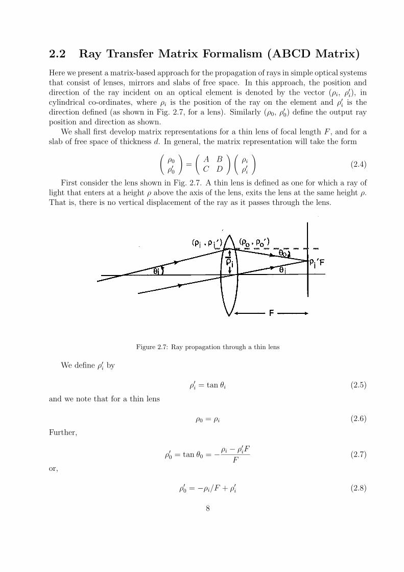
Here we present a matrix-based approach for the propagation of rays in simple optical systemsthat consist of lenses, mirrors and slabs of free space. In this approach, the position anddirection of the ray incident on an optical element is denoted by the vector (ρi, ρ′i), incylindrical co-ordinates, where ρi is the position of the ray on the element and ρ′i is thedirection defined (as shown in Fig. 2.7, for a lens). Similarly (ρ0, ρ′0) define the output rayposition and direction as shown.

We shall first develop matrix representations for a thin lens of focal length F , and for aslab of free space of thickness d. In general, the matrix representation will take the form

(ρ0

ρ′0

)=

(A BC D

) (ρi

ρ′i

)(2.4)

First consider the lens shown in Fig. 2.7. A thin lens is defined as one for which a ray oflight that enters at a height ρ above the axis of the lens, exits the lens at the same height ρ.That is, there is no vertical displacement of the ray as it passes through the lens.

Figure 2.7: Ray propagation through a thin lens

We define ρ′i by

ρ′i = tan θi (2.5)

and we note that for a thin lens

ρ0 = ρi (2.6)

Further,

ρ′0 = tan θ0 = −ρi − ρ′iFF

(2.7)

or,

ρ′0 = −ρi/F + ρ′i (2.8)

8

The latter two equations (Eqns. 2.6 and 2.8) can be rewritten in the desired matrix algebraform as

(ρ0

ρ′0

)=

(1 0− 1

F1

) (ρi

ρ′i

)(2.9)

Thus Ml, the transformation matrix for a lens can be written as

Ml =

(1 0− 1

F1

)(2.10)

Slab of Free space

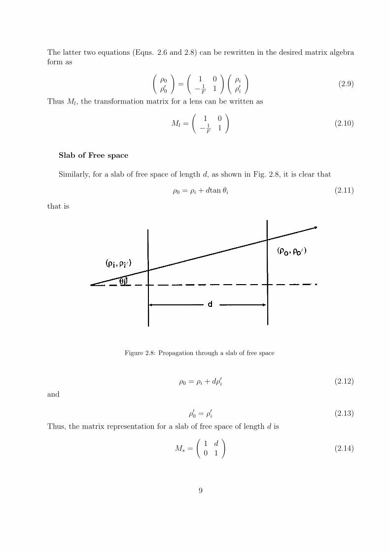
Similarly, for a slab of free space of length d, as shown in Fig. 2.8, it is clear that

ρ0 = ρi + dtan θi (2.11)

that is

Figure 2.8: Propagation through a slab of free space

ρ0 = ρi + dρ′i (2.12)

and

ρ′0 = ρ′i (2.13)

Thus, the matrix representation for a slab of free space of length d is

Ms =

(1 d0 1

)(2.14)

9

Slab of Free Space followed by a Lens

Combining the above results, we find that propagation through a section of free space ofthickness d followed by a lens of focal length F (see Fig. 2.9) can be described by the matrixequation (

ρ0

ρ′0

)=

(1 0− 1

F1

) (1 d0 1

) (ρi

ρ′i

)(2.15)

Thus, the ABCD matrix representation for free space followed by a lens is

d F

(ρi ,ρi')

(ρo ,ρo')oo

Figure 2.9: Slab of free space followed by a lens.

Msl =

(1 d− 1

F1− d

F

)(2.16)

.

Lens Followed by a Slab of free space

Similarly for a lens followed by a slab of free space (see Fig. 2.10) we have

dF

(ρi ,ρi')

(ρo ,ρo')o o

Figure 2.10: Lens followed by a slab of free space.

(ρ0

ρ′0

)=

(1 d0 1

) (1 0− 1

F1

) (ρi

ρ′i

)(2.17)

which implies that

10

Mls =

(1− d

Fd

− 1F

1

)(2.18)

.

From Eqns. 2.43 and 2.18 it should be clear that the matrices do not commute and so theorder of multiplication is important. Note that for rays propagating left to right, the matrixelements are written down right to left. And, if the matrices are multiplied in the incorrectorder, the effect is an interchange of the elements on the main diagonal. By multiplyingsuccessive free-space and lens ABCD matrices, one can see how a complex, multi-elementwave-guiding system, as shown later in Figure 2.15, can be quickly and easily analyzed.Similarly, the ABCD approach can be used to analyze imaging systems for ray tracing ingeneral.

2.2.1 Multiple Lens Systems

First let us again consider the single lens optical system shown in Fig. 2.11 where d1 is thedistance of the input object plane P1 from the lens and d2 is the distance of the output planeP2 (not necessarily object and image planes, respectively).

d1 F1

(ρi ,ρi')

(ρo ,ρo')

d2P1 P2

input plane output plane

o o

Figure 2.11: Single-lens optical system

This system can be thought of as two cascaded components: a slab of thickness d1 followedby a lens and slab of free space of thickness d2. Thus we have

(ρ0

ρ′0

)=

(1 d2

0 1

) (1 d1

− 1F

1− d1

F

) (ρi

ρ′i

)(2.19)

and so

Msystem =

(1− d2

Fd1 + d2 − d1d2

F

− 1F

1− d1

F

)(2.20)

In the special case where P1 and P2 are object and image planes respectively, ρo must beindependent of ρ′i. That is, all rays leaving a specific point ρi in the input plane P1 mustpass through a single specific point in the P2 (output) plane irrespective of their direction,

11

ρ′i, with which they left the P1 plane. Thus, by inspection of the ABCD matrix, it is clearthat when the imaging condition is satisfied, B = 0. This means that

d1 + d2 − d1d2

F= 0 (2.21)

d1

d1d2

+d2

d1d2

− 1

F= 0 (2.22)

hence

1

d2

+1

d1

=1

F(2.23)

as expected.

The lateral magnification, with B = 0, is thus equal to A. That is,

M =ρo

ρi

= A = (1− d2

F) (2.24)

= (1− [1 +d2

d1

]) (2.25)

= −d2

d1

(2.26)

as expected. Negative magnification means that the image is inverted relative to the object.In this single-lens case, a negative value for d2 would mean that the image is virtual and ison the same side of the lens as the object.

2.2.2 Two-Lens Optical System

The two-lens optical system shown in Fig. 2.12 is very popular in many projector systems.The telescope and microscope are special cases. It is clear that this system can be thoughtof as the single-lens system followed by a lens-slab combination.

d1

F1

(ρi ,ρi')

(ρo ,ρo')

P1 P2

input plane output planeF2

d2 d3

o o

Figure 2.12: Two-lens optical system

12

It therefore follows that(

ρ0

ρ′0

)=

(1− d3

F2d3

− 1F2

1

) (1− d2

F1d1 + d2 − d1d2

F1

− 1F1

1− d1

F1

) (ρi

ρ′i

)(2.27)

hence,

Msystem =

((1− d3

F2)(1− d2

F1)− d3

F1(1− d3

F2)(d1 + d2 − d1d2

F1) + d3(1− d1

F1)

− 1F2

(1− d2

F1)− 1

F1− 1

F2(d1 + d2 − d1d2

F1) + (1− d1

F1)

)(2.28)

When this system is setup for imaging, ρo is independent of ρ′i (B = 0). In this case, wehave

d1 + d2 − d1d2

F1

− d1d3

F2

− d2d3

F2

− d1d2d3

F1F2

− d1d3

F1

+ d3 = 0 (2.29)

or

1

d3

=1F2

( 1d1

+ 1d2− 1

F1)− 1

d2( 1

d1− 1

F1)

( 1d1

+ 1d2− 1

F1)

(2.30)

or

d3 =

[1

F2

− 1

d2

( 1d1− 1

F1)

( 1d1

+ 1d2

+ 1F1

)

]−1

(2.31)

The magnification M2l is equal to A when B = 0.

M2l = (1− d3

F2

)(1− d2

F1

)− d3

F1

(2.32)

= d3(d2

F1F2

− 1

F1

− 1

F2

) + 1− d2

F1

(2.33)

Even though d1 does not appear explicitly in Eqn. 2.33, M is not independent of d1 sinced1 determines d3. To find the dependence of M on d1 we can express d3 in terms of d1, aspreviously shown (2.30) and we find that

M2l = 1− d2

F1

+( 1

d1+ 1

d2− 1

F1)( d2

F1F2− 1

F1− 1

F2)

1F2

( 1d1

+ 1d2− 1

F1)− 1

d2( 1

d1− 1

F1)

(2.34)

In the special imaging case where F1 = F2 = F and d1 = d3 we see that M = −1 as expected.Returning to the special case of a telescope (which is not a P1 to P2 imaging system) so wemust go back to Eqn. 2.28, we note that since

ρ′ = Cρi + Dρ′i (2.35)

the angular magnification Mtel will be D when C = 0. Indeed for the telescope sinced2 = F1 + F2, we see from Eqn. 2.28 that

13

C = − 1

F2

(1− d2

F1

)− 1

F1

= 0 (2.36)

This implies that the angular magnification Mtel is

Mtele = D = − 1

F2

(d1 + d2 − d1d2

F1

) + (1− d1

F1

) (2.37)

= −F1

F2

(2.38)

when d2 = F1 + F2 and is also independent of d1 as expected.

2.3 Telescopes

In the refractive telescope shown in Fig. 2.13, it is presumed that the object is very far awayand that it subtends a half-angle α to the unaided eye. Note that Fig. 2.13 shows onlythe set of rays (from from the ”bottom” of the distant object). In the standard telescopeconfiguration the objective and eyepiece have a common focus, as shown. The focal lengthof the objective F1 is always greater than the focal length of the eyepiece and it produces avirtual image at infinity.

α'

F1

objective

intermediate

image

α

eye

F2

F2

eyepiece

Figure 2.13: Ray diagram for a telescope.

The effect of the telescope is to increase the angle subtended at the eye from α to α′.The magnification is defined by

M =Angle image subtends at the eye with telescope

Angle object subtends at the unaided eye=

α′

α= −F1

F2

(2.39)

This can be seen from Fig. 2.13 by drawing in the special ray (dashed line) that passesthrough the intermediate image and is parallel to the principal axis in the region betweenthe lenses. This ray must clearly pass through the back focus of the eyepiece and the frontfocus of the objective. It then follows that tan α′ = h/F2 and tan α = h/F1, where h is theheight of the intermediate image, and with the small angle approximation it follows that

14

M =α′

α= −F1

F2

(2.40)

Many variants of the standard telescope exist. For example, the eyepiece may be anegative lens (Galilean telescope), mirrors may be used instead of lenses, or the objectivemay be a mirror and the eyepiece a lens.

2.4 Microscopes

With a microscope, it is presumed that the object is a distance F1+ε in front of the objective(of focal length F1) and that ε is small. That is, the system is set up so that the intermediateimage is formed near the focal plane of the eyepiece whose focal length is F2 (see Fig. 2.14).The separation g (g >> 0, F1) between the focus of the objective and that of the eyepieceis called the barrel length and is typically 160 mm. Also, the focal length of the objective ismuch smaller than that of the eyepiece (F1 < F2).

α'

F1+ ε

y

F1<F

2

g

intermediate image

F2

F2 eye

F1

. .δ

objective

eyepiece

Figure 2.14: Ray diagram for a microscope

In this case, we define α, the angle subtended by the object at the unaided eye to beα ≈ y

dminwhere y is object size, and dmin is the nearest distance for sharp seeing with the

unaided eye (typically about 25 cm for a young person). By drawing in the ray from theintermediate image that passes undeviated through the center of the eyepiece, we can showthat the angular magnification, M , is given by

M =α′

α≈ −gdmin

F1F2

(2.41)

Alternatively, you can derive the magnification by first showing that the effective focal lengthof the combination of lenses is F1F2

gand then assuming the image is at dmin. In practice the

eyepiece is adjusted for comfortable viewing, so the image is not at infinity.

15

2.5 Lens Waveguide

The lens waveguide (illustrated in Fig. 2.15) is a convenient means of studying how lightpropagates between two mirrors separated by a distance d. This is because reflection ata mirror with radius of curvature R is equivalent, except for the folded path, to passagethrough a lens of focal length R/2.

ρs

ρs+1

Figure 2.15: Propagation through a lens waveguide

We note that the lens waveguide consists of lenses and slabs of free-space. Thus theABCD ray-matrix approach can be used to analyze this system. From the previous resultswe know that propagation through a section of free space of thickness d followed by a lensof focal length F (see Eqn. 2.15) is described by the matrix equation.

(ρ0

ρ′0

)=

(1 0− 1

F1

) (1 d0 1

) (ρi

ρ′i

)(2.42)

That is, the matrix for free space followed by a lens is

Msl =

(1 d

−1/F 1− d/F

)(2.43)

Returning to the lens waveguide of Fig. 2.15, notice that the system is spatially periodic inthe z direction with the unit cell described as shown. Our goal now is to find the relationshipbetween d, F1 and F2 such that any ray passing through this system is confined (i.e., it doesnot escape). That is, ρs remains finite.

So, for propagation over the basic unit shown in Fig. 2.15, we have using Eqn. 2.43

(ρs+1

ρ′s+1

)=

(1 d

−1/F1 1− d/F1

) (1 d

−1/F2 1− d/F2

) (ρs

ρ′s

)(2.44)

This is of the form

16

(ρs+1

ρ′s+1

)=

(A BC D

) (ρs

ρ′s

)(2.45)

where

A = 1− d/F2 (2.46)

B = d(2− d/F2) (2.47)

C = −[

1

F1

+1

F2

(1− d

F1

)

](2.48)

D = − d

F1

+ (1− d

F1

)(1− d

F2

) (2.49)

= 1− 2d

F1

− d

F2

+d2

F1F2

(2.50)

From Eqn. 2.45 it follows that

ρs+1 = Aρs + Bρ′s (2.51)

or

ρ′s =1

B(ρs+1 − Aρs) (2.52)

Therefore, by induction,

ρ′s+1 =1

B(ρs+2 − Aρs+1) (2.53)

but from Eqn. 2.45, we also have

ρ′s+1 = Cρs + Dρ′s (2.54)

Substituting for ρ′s and ρ′s+1 using Eqns. 2.53 and 2.54 we find that

1

Bρs+2 − A

Bρs+1 − Cρs − D

Bρs+1 +

DA

Bρs = 0 (2.55)

and noting that the determinant of the ABCD matrix is unity; that is,

AD −BC = 1 (2.56)

we find that the evolution of a ray through the guide obeys an equation of the form

ρs+2 − 2bρs+1 + ρs = 0 (2.57)

where

b =1

2(A + D) = (1− d

F1

− d

F2

+d2

2F1F2

) (2.58)

17

A solution to the difference equation (Eqn. 2.58) is of the form

ρs = ρ0ejsφ (2.59)

Plugging this solution back into Eqn. 2.58, we get

ejsφ[ej2φ − 2bejφ + 1] = 0 (2.60)

And solving the quadratic equation within the parentheses of the above equation, we find

ejφ = b± j(1− b2)1/2 (2.61)

Hence, b is of the form

b = cos φ (2.62)

The condition for confinement is that φ be real, so that ρs oscillates ( see Eqn. 2.59) ratherthan grows or diminishes. That is, we want

−1 ≤ cos φ ≤ 1 (2.63)

or

−1 ≤ b ≤ 1 (2.64)

or

−1 ≤ (1− d

F1

− d

F2

+d2

2F1F2

) ≤ 1 (2.65)

Adding 1 to all sections of this relationship and dividing by 2 yields

0 ≤ (1− d

2F1

)(1− d

2F2

) ≤ 1 (2.66)

Because of the similarity between a cavity of two mirrors and a lens waveguide, Eqn. 2.66is the condition that must be satisfied to confine a beam inside a laser cavity. Since therelationship between a lens of focal length F and a mirror of focal length F is that theradius of curvature of the equivalent mirror is 2F , we can transform the lens waveguideconfinement condition above into the laser resonator stability condition below.

0 ≤ (1− d

R1

)(1− d

R2

) ≤ 1 (2.67)

Figure 2.16 is a graphical plot of the boundaries of Eqn. 2.67 depicting the various regionsof stability and the points that correspond to a few of the standard resonator geometries.Also, given a laser cavity which satisfies the stability condition (Eqn. 2.67) it can be shownthat if φ satisfies the condition

2nφ = 2mπ (2.68)

where n and m are integers, the ray will return to its starting point after n round trips andthus will constantly retrace the same pattern on the mirrors.

18

Low Loss

Low Loss

High LossHigh Loss

High Loss

Concentric

d = R + R

1 2

d/R = 1

High Loss

1

plane parallel

d/R = 12

d/R 2

d/R 1

Confocal

Systems

Confocal Systems

Symmetric

Confocal

d = R = R

21

Figure 2.16: Regions of Stability for Laser Cavities - Adapted from A. Yariv, Optical Electronics in ModernCommunications, 5th Ed. New York: Oxford University Press, 1997

19