Class Notes Intermediate Macroeconomics Li Gan

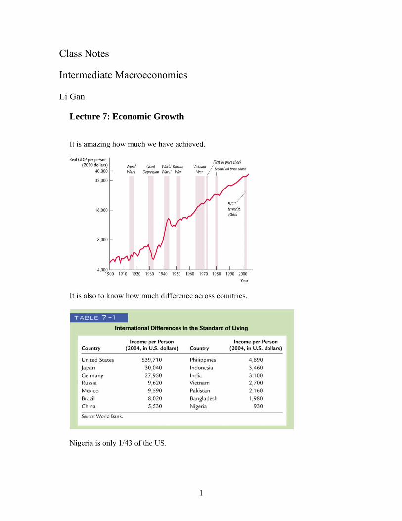
Lecture 7: Economic Growth It is amazing how much we have achieved.

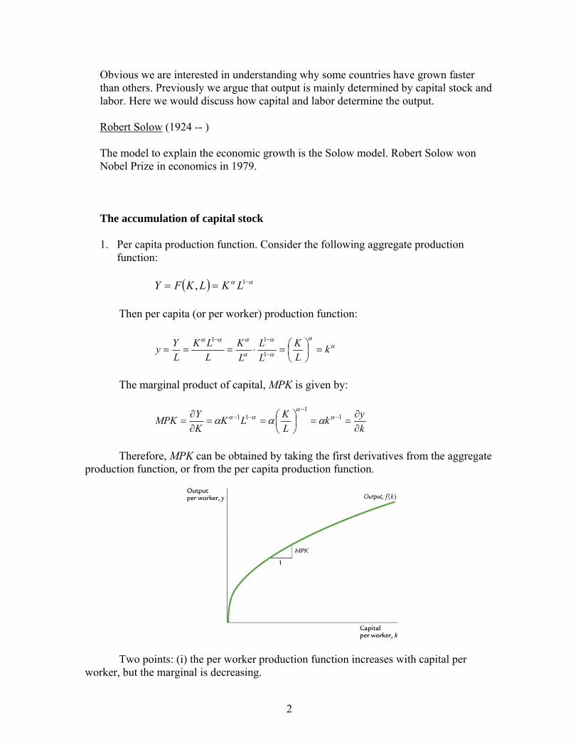
It is also to know how much difference across countries.

Nigeria is only 1/43 of the US.

1

Obvious we are interested in understanding why some countries have grown faster than others. Previously we argue that output is mainly determined by capital stock and labor. Here we would discuss how capital and labor determine the output. Robert Solow (1924 -- ) The model to explain the economic growth is the Solow model. Robert Solow won Nobel Prize in economics in 1979.

The accumulation of capital stock 1. Per capita production function. Consider the following aggregate production

function:

( ) αα −== 1, LKLKFY Then per capita (or per worker) production function:

αα

α

α

α

ααα

kLK

LL

LK

LLK

LYy =⎟

⎠⎞

⎜⎝⎛=⋅=== −

−−

1

11

The marginal product of capital, MPK is given by:

kyk

LKLK

KYMPK

∂∂

==⎟⎠⎞

⎜⎝⎛==

∂∂

= −−

−− 11

11 αα

αα ααα

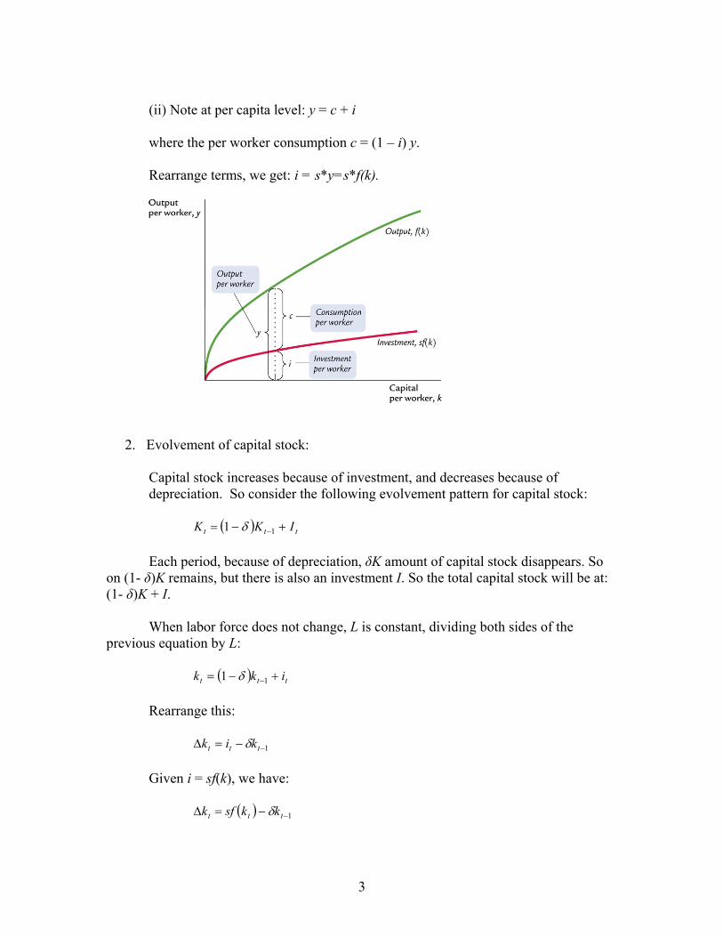
Therefore, MPK can be obtained by taking the first derivatives from the aggregate production function, or from the per capita production function.

Two points: (i) the per worker production function increases with capital per worker, but the marginal is decreasing.

2

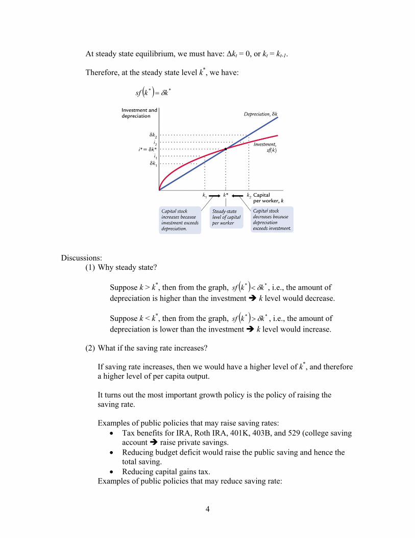
(ii) Note at per capita level: y = c + i where the per worker consumption c = (1 – i) y. Rearrange terms, we get: i = s*y=s*f(k).

2. Evolvement of capital stock:

Capital stock increases because of investment, and decreases because of depreciation. So consider the following evolvement pattern for capital stock: ( ) ttt IKK +−= −11 δ

Each period, because of depreciation, δK amount of capital stock disappears. So on (1- δ)K remains, but there is also an investment I. So the total capital stock will be at: (1- δ)K + I. When labor force does not change, L is constant, dividing both sides of the previous equation by L: ( ) ttt ikk +−= −11 δ Rearrange this: 1−−=Δ ttt kik δ Given i = sf(k), we have: ( ) 1−−=Δ ttt kksfk δ

3

At steady state equilibrium, we must have: Δkt = 0, or kt = kt-1. Therefore, at the steady state level k*, we have: ( ) ** kksf δ=

Discussions:

(1) Why steady state?

Suppose k > k*, then from the graph, ( ) ** kksf δ< , i.e., the amount of depreciation is higher than the investment k level would decrease. Suppose k < k*, then from the graph, ( ) ** kksf δ> , i.e., the amount of depreciation is lower than the investment k level would increase.

(2) What if the saving rate increases?

If saving rate increases, then we would have a higher level of k*, and therefore a higher level of per capita output. It turns out the most important growth policy is the policy of raising the saving rate. Examples of public policies that may raise saving rates:

• Tax benefits for IRA, Roth IRA, 401K, 403B, and 529 (college saving account raise private savings.

• Reducing budget deficit would raise the public saving and hence the total saving.

• Reducing capital gains tax. Examples of public policies that may reduce saving rate:

4

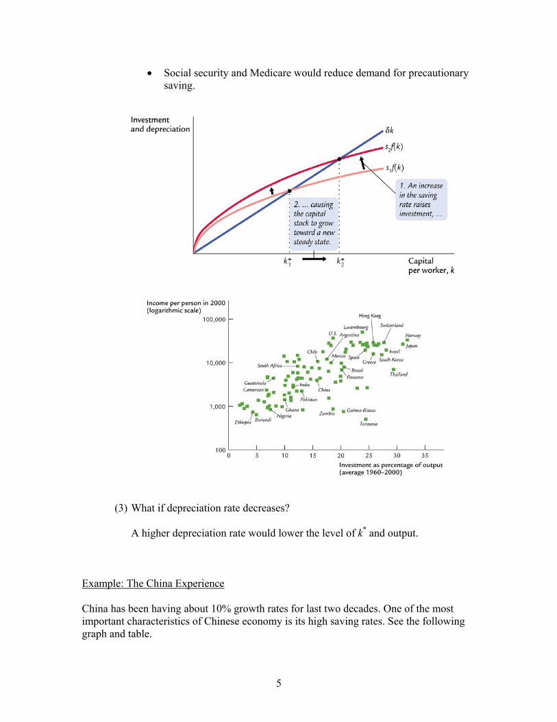
• Social security and Medicare would reduce demand for precautionary saving.

(3) What if depreciation rate decreases?

A higher depreciation rate would lower the level of k* and output. Example: The China Experience China has been having about 10% growth rates for last two decades. One of the most important characteristics of Chinese economy is its high saving rates. See the following graph and table.

5

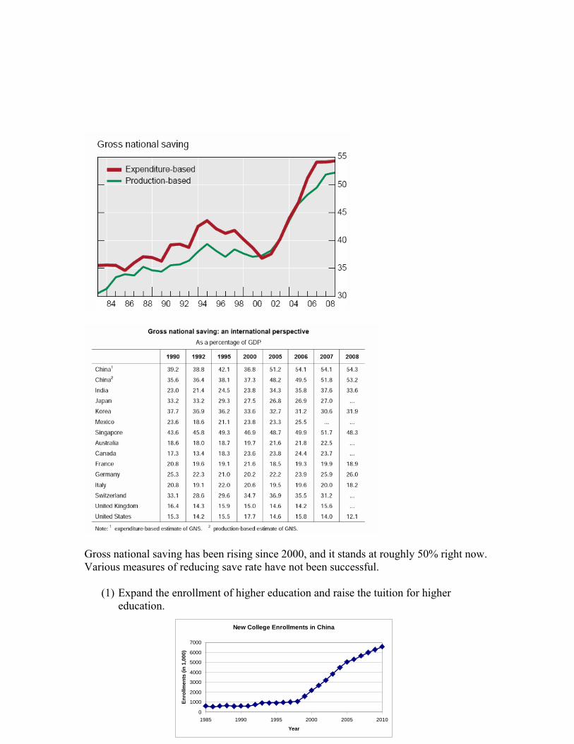
Gross national saving has been rising since 2000, and it stands at roughly 50% right now. Various measures of reducing save rate have not been successful.

(1) Expand the enrollment of higher education and raise the tuition for higher education.

6

New College Enrollments in China

4000

5000

6000

7000

(in

1,00

0)

0

1000

2000

3000

1985 1990 1995 2000 2005 2010

Year

Enro

llmen

ts

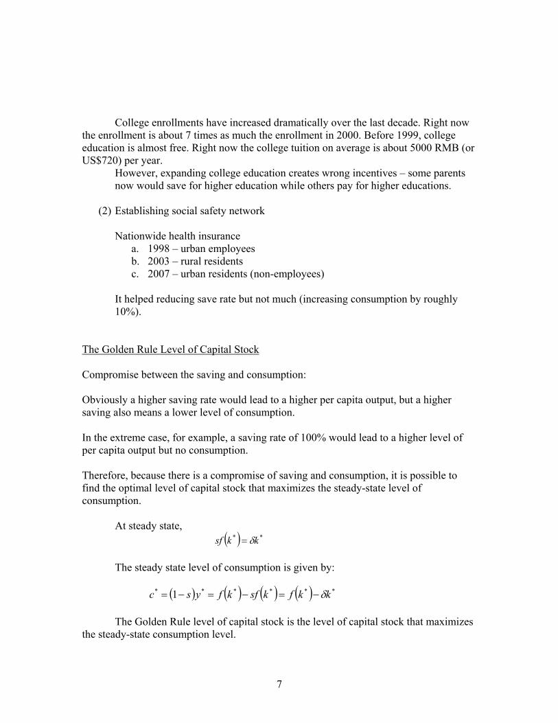
College enrollments have increased dramatically over the last decade. Right nothe enrollment is about 7 times as much the enrollment in 2000. Before 1999, college education is almost f

w

ree. Right now the college tuition on average is about 5000 RMB (or US$72

s ow would save for higher education while others pay for higher educations.

(2) stablishing social safety network

Nats

c. 2007 – urban residents (non-employees)

reducing save rate but not much (increasing consumption by roughly 10%).

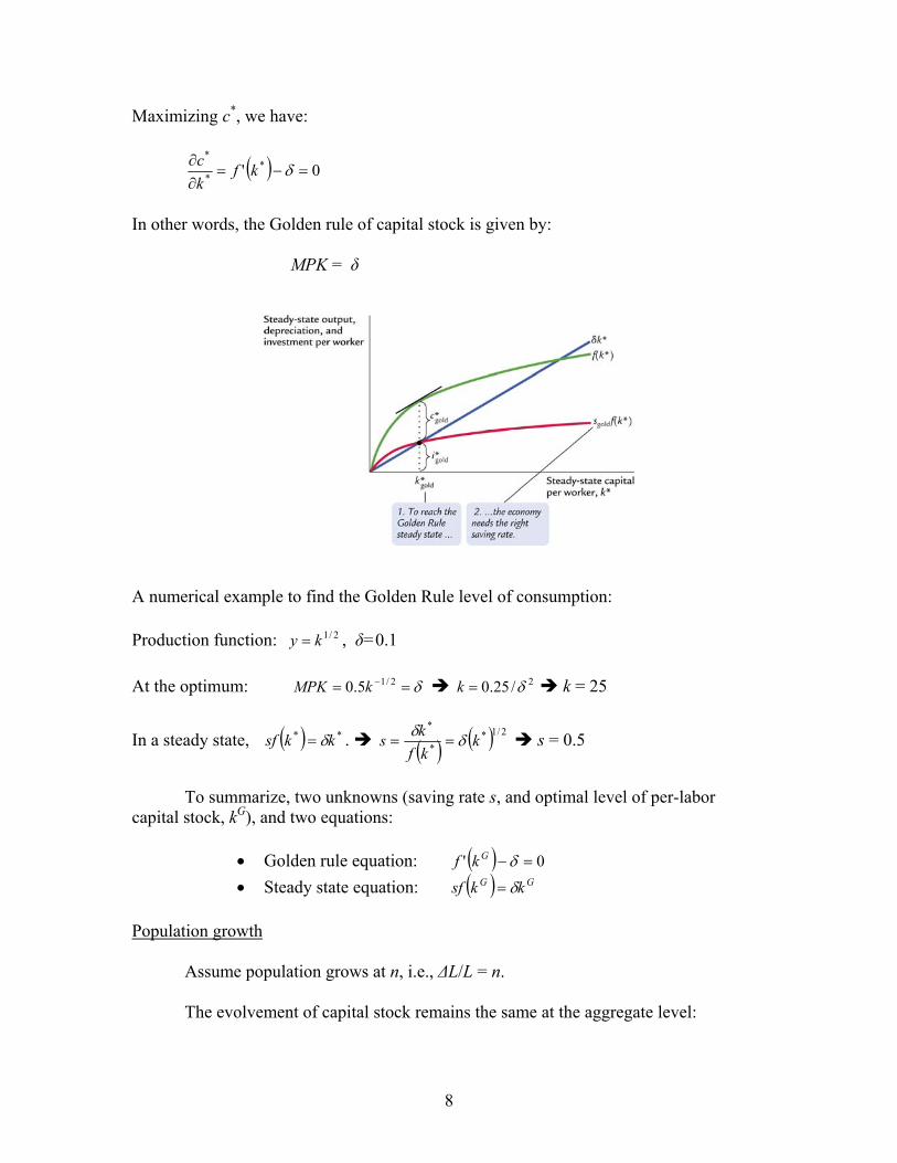
he Golden Rule Level of Capital Stock

0) per year. However, expanding college education creates wrong incentives – some parentn E

ionwide health insurance a. 1998 – urban employeeb. 2003 – rural residents

It helped

T

ompromise between the saving and consumption:

her per capita output, but a higher aving also means a lower level of consumption.

ng rate of 100% would lead to a higher level of er capita output but no consumption.

ible to at maximizes the steady-state level of

onsumption.

C Obviously a higher saving rate would lead to a higs In the extreme case, for example, a savip Therefore, because there is a compromise of saving and consumption, it is possfind the optimal level of capital stock thc At steady state,

( ) ** kksf δ= The steady state level of consumption is given by:

( ) ( ) ( ) ( ) ****** 1 kkfksfkfysc δ−=−=−=

ital stock is the level of capital stock that maximizes e steady-state consumption level.

The Golden Rule level of capth

7

Maximizing c*, we have:

( ) 0' * * −=∂

δkfk

*

=∂c

other words, the Golden rule of capital stock is given by:

MPK = δ

In

A numerical example to find the Golden Rule level of consumption:

roduction function: , δ=0.1

t the optimum: k = 25

In a steady state,

P 2/1ky =

δ== − 2/15.0 kMPK 2/25.0 δ=k A

( ) ** kksf δ= . ( ) ( ) 2/1**

*

kkfks δδ

== s = 0.5

(saving rate s, and optimal level of per-labor

wo equations:

To summarize, two unknowns capital stock, kG), and t

( )• Golden rule equation: 0' =−δGkf

• Steady state equation: ( ) GG kksf δ= Population growth

Assume population grows at n, i.e., ΔL/L = n.

The evolvement of capital stock remains the same at the aggregate level:

8

ΔK = I – δK

The evolvement of the per-labor capital stock now becomes:

( ) ( )knksfnkki

LK

LL

LKI

LLK

LK

LKk

+−=−−=

⋅Δ

−−

=

Δ−

Δ=⎟

⎠⎞

⎜⎝⎛Δ=Δ

δδ

δ

2

Note: here we apply the total differentiation formula.

The steady state is determined by Δk=0

Therefore, at the steady state,

( ) ( ) ** knksf += δ Intuitively, the population growth serves in a similar role as the depreciation atper capita l

the evel. Higher the population growth rate, the per capita capital stock would

ecrease.

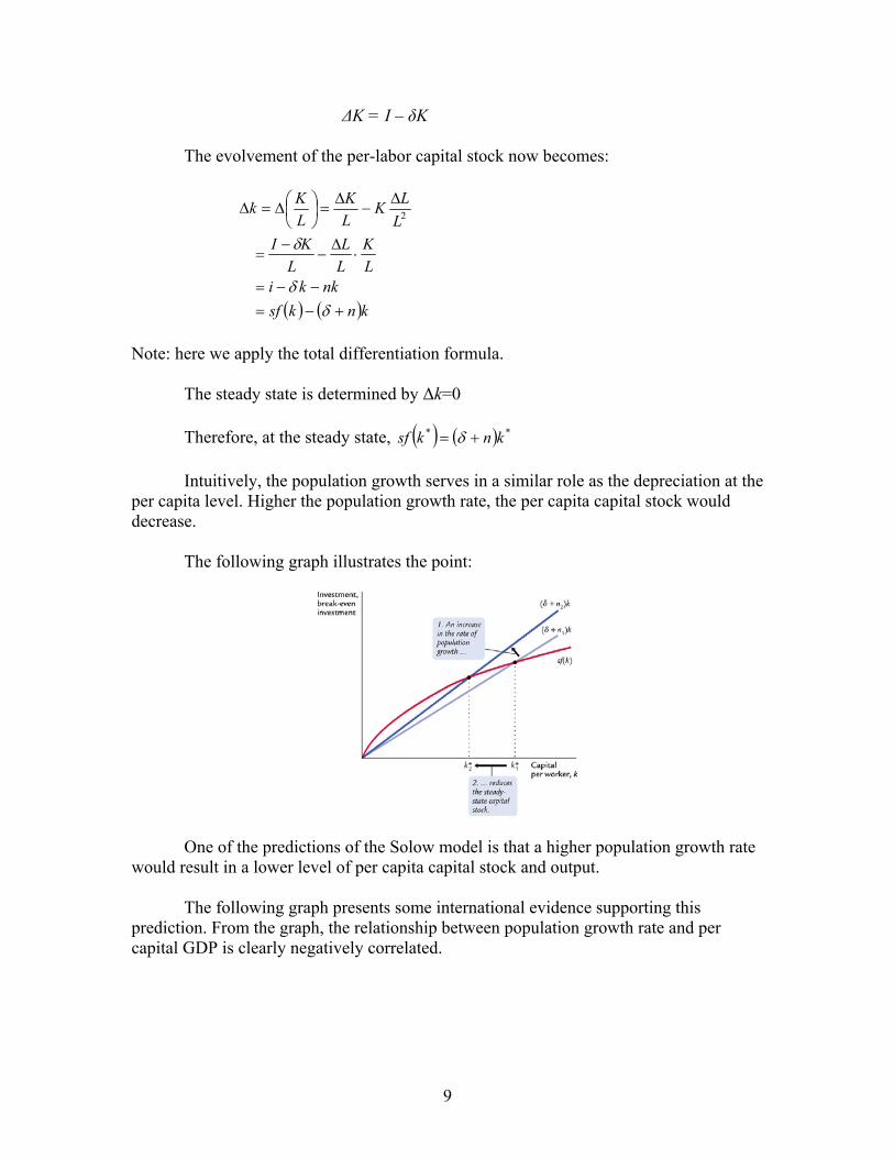
The following graph illustrates the point:

d

One of the predictions of the Solow model is that a higher population growth rate

ould result in a lower level of per capita capital stock and output.

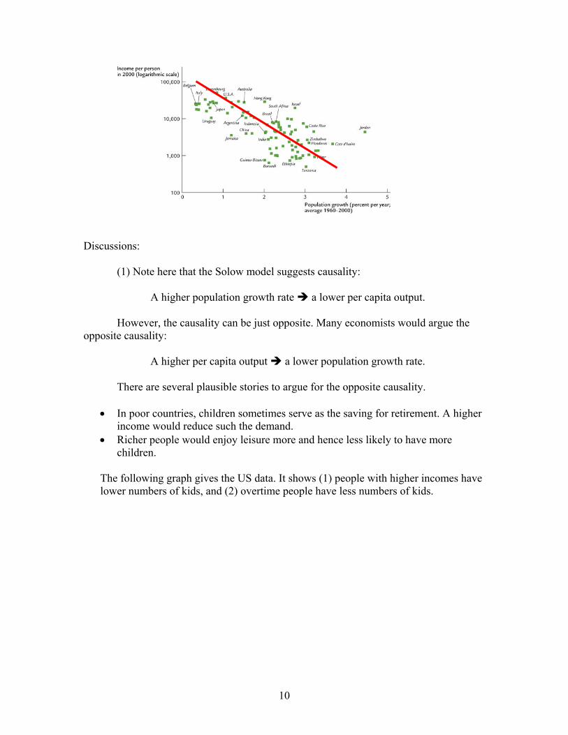
etween population growth rate and per apital GDP is clearly negatively correlated.

w The following graph presents some international evidence supporting this prediction. From the graph, the relationship bc

9

Discussions:

(1) Note here that the Solow model suggests causality:

A higher population growth rate a lower per capita output. However, the causality can be just opposite. Many economists would argue the opposite causality: A higher per capita output a lower population growth rate. There are several plausible stories to argue for the opposite causality.

• In poor countries, children sometimes serve as the saving for retirement. A higher income would reduce such the demand.

• Richer people would enjoy leisure more and hence less likely to have more children.

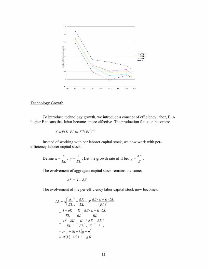
The following graph gives the US data. It shows (1) people with higher incomes have lower numbers of kids, and (2) overtime people have less numbers of kids.

10

Technology Growth

To introduce technology growth, we introduce a concept of efficiency labor, E. A higher E means that labor becomes more effective. The production function becomes: ( ) ( ) αα −== 1, ELKELKFY

Instead of working with per laborer capital stock, we now work with per-efficiency laborer capital stock.

Define ELYy

ELKk == , . Let the growth rate of E be:

EEg Δ

= .

The evolvement of aggregate capital stock remains the same: ΔK = I – δK The evolvement of the per-efficiency labor capital stock now becomes:

( )

( )( ) ( )kgnksf

ngkkysLL

EE

ELK

ELKsY

ELLELE

ELK

ELKI

ELLELEK

ELK

ELKk

++−=+−−⋅=

⎟⎠⎞

⎜⎝⎛ Δ

+Δ

⋅−−

=

Δ⋅+⋅Δ⋅−

−=

Δ⋅+⋅Δ−

Δ=⎟

⎠⎞

⎜⎝⎛Δ=Δ

δδ

δ

δ

2

11

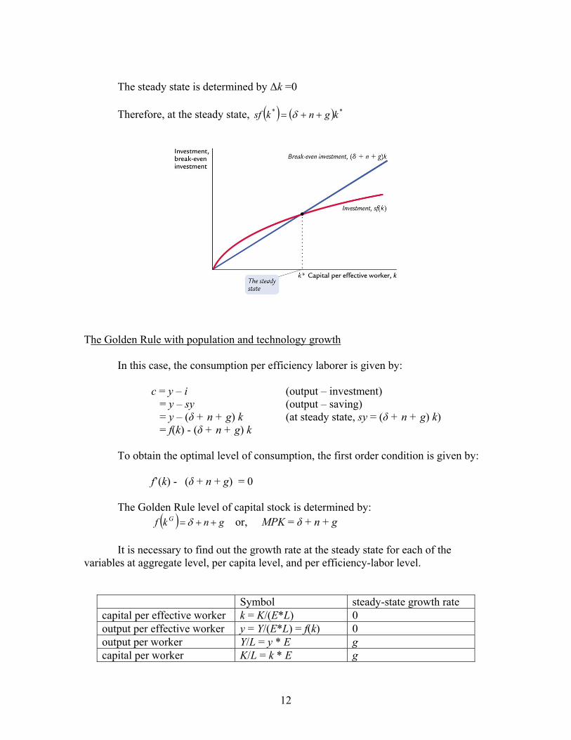
The steady state is determined by Δk =0

Therefore, at the steady state, ( ) ( ) ** kgnksf ++= δ

The Golden Rule with population and technology growth In this case, the consumption per efficiency laborer is given by: c = y – i (output – investment) = y – sy (output – saving) = y – (δ + n + g) k (at steady state, sy = (δ + n + g) k) = f(k) - (δ + n + g) k To obtain the optimal level of consumption, the first order condition is given by: f’(k) - (δ + n + g) = 0 The Golden Rule level of capital stock is determined by: ( ) gnkf G ++= δ or, MPK = δ + n + g

It is necessary to find out the growth rate at the steady state for each of the variables at aggregate level, per capita level, and per efficiency-labor level.

Symbol steady-state growth rate capital per effective worker k = K/(E*L) 0 output per effective worker y = Y/(E*L) = f(k) 0 output per worker Y/L = y * E g capital per worker K/L = k * E g

12

total output Y = y * (E * L) g+n total capital K = k * (E * L) g+n

If we want per worker output to grow when the economy is at the steady state, the only way is to have technology growth. Discussions:

(1) To calculate the Golden Rule saving rate, two equations and two unknowns:

• The Golden rule equation: ( ) gnkf G ++= δ' • Steady state equation: ( ) ( ) GG kgnksf ++= δ

Numerical example: In the US, it is typically assumed that (i) the capital stock is 2.5 times one year’s GDP; (ii) Depreciation of capital is about 10% of GDP; and (iii) Capital income is about 30% of GDP. What is the Golden-rule saving rate?

We have: k = 2.5y δk = 0.1y MPK*k = 0.3y The depreciation rate is given by: δ = 0.1y/2.5y = 0.04 And MPK is given by: MPK = 0.3y/k = 0.3y/2.5y = 0.12 Therefore, current MPK = 0.12.

The Golden rule level: gnMPK G ++= δ Given that n = 0.01, δ = 0.04, and g < 0.07 We have: 12.0=< MPKMPK G

The current MPK is too high the current steady state capital stock k*:

Gkk =*

What is the Golden Rule saving rate? We have: 0.3y/k = δ + n + g, or k(δ + n + g) = 0.3y Since k(δ + n + g) = sy, we must have:

13

3.0=Gs

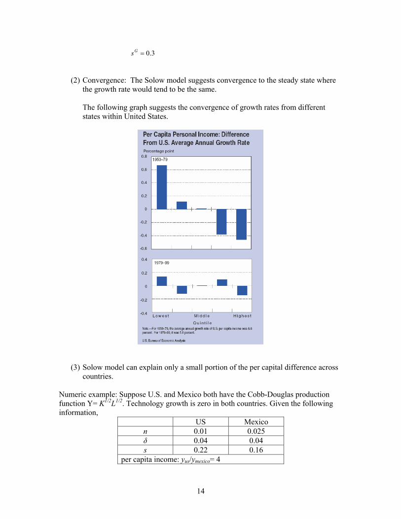
(2) Convergence: The Solow model suggests convergence to the steady state where the growth rate would tend to be the same.

The following graph suggests the convergence of growth rates from different states within United States.

(3) Solow model can explain only a small portion of the per capital difference across countries.

Numeric example: Suppose U.S. and Mexico both have the Cobb-Douglas production function Y= K1/2L1/2. Technology growth is zero in both countries. Given the following information,

US Mexico n 0.01 0.025 δ 0.04 0.04 s 0.22 0.16

per capita income: yus/ymexico= 4

14

What is the ratio of the two countries according to the Solow model? At the steady state,

sy = (n+δ)k ( )knsk δ+=2/1

( )δ+= nssk /2/1

y = s/(n+δ) Therefore,

79.1

04.0025.016.0

04.001.022.0

=

+

+=

+

+=

δ

δ

Mexico

Mexico

US

US

Mexico

US

ns

ns

yy

However, we know that yus/ ymexico= 4. So the Solow model can only explain a small portion of the ratio. It turns out that Solow model can only explain a small potion of the difference across countries, especially across developing and developed countries. (a) One possibility is that the two countries have different level of E. Consider the Solow model with technology growth. At the steady state, we have: sy = (n+δ+g)k In this case, please note that y = Y/(E*L), and k = K/(E*L). Assume g = 0, then we have:

US

Mexico

US

Mexico

MexicoMexico

USUS

MexicoMexico

Mexico

USUS

US

Mexico

US

EE

EE

LYLY

LEY

LEY

yy

⋅=⋅=== 4//

79.1

Therefore, 4475.479.1

==US

Mexico

EE

In another word, a US worker is twice as productive as the Mexican worker (at the given level of capital stock). (b) Another possibility is to have different production function. For Mexico, y=kβ.

15

s kβ = (δ+n) k. So k1-β = s/(δ+n). y = [s/(δ+n)] β/(1-β). yus/ymexico = 4.4/2.46 β/(1-β) = 4.

Solve for β, we get β = 0.096. So in Mexico, the share of capital could potentially be very small. Endogenous Growth Theory

(1) One sector endogenous growth model:

The basic idea: investment, especially investment in R&D would lead to more productivity.

Let E = B*K/L this is to say that labor efficiency depends on the how much capital stock per worker has. A is a scaling factor.

Given this, the total output function becomes: Y = Kα(E*L)1-α = Kα(B*K/L* L)1-α = B1-αK = AK

where A = B1-α, a constant. Again, consider the evolvement of capital stock: ΔK = sY – δK = sAK – δK = (sA – δ)K The growth rates of the total output and the total capital stock are: ΔK/K = sA – δ ΔY/Y = sA – δ

In the following graph, sA > δ , there will be no steady state, capital stock will continue to grow.

16

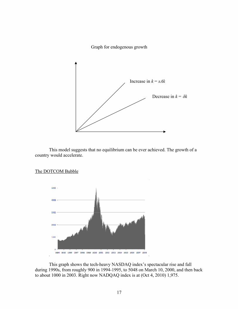
Graph for endogenous growth

Increase in k = sAk

Decrease in k = δk

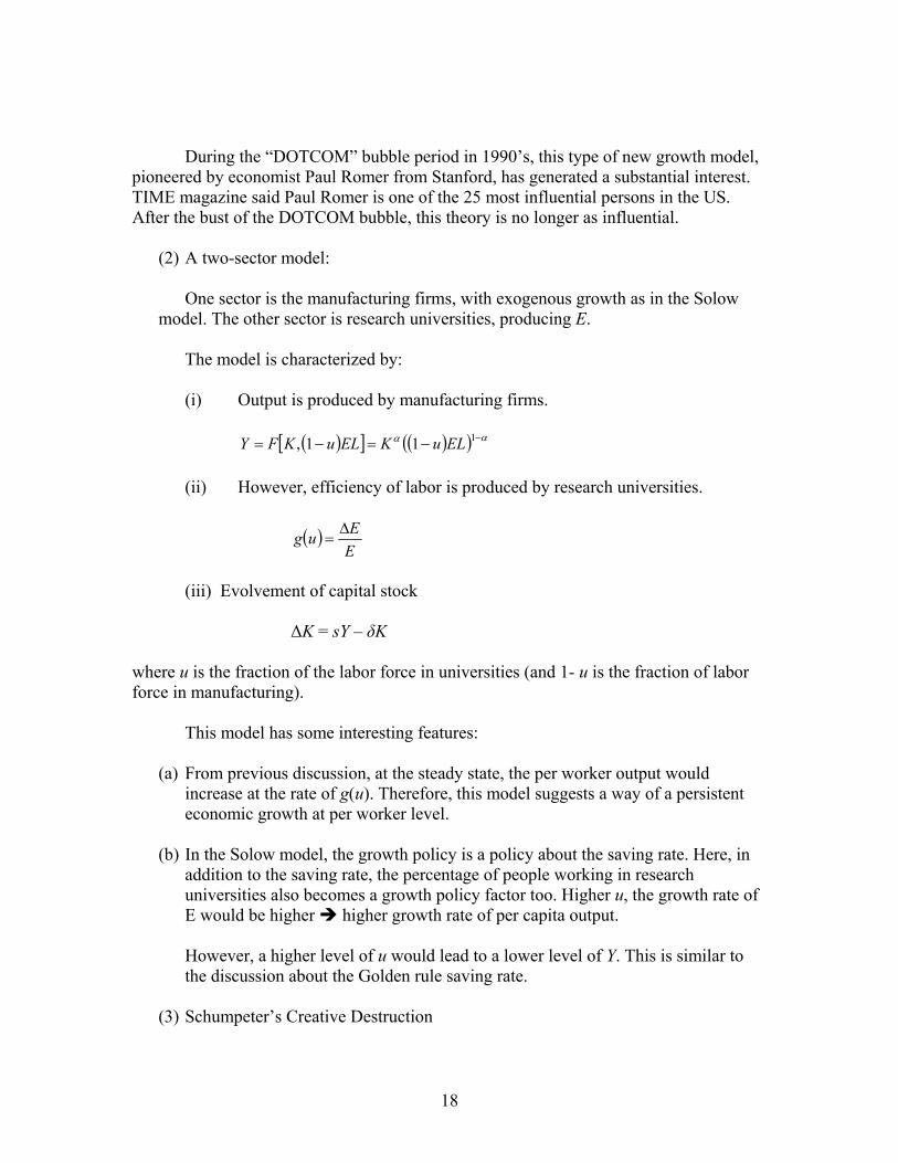
This model suggests that no equilibrium can be ever achieved. The growth of a country would accelerate. The DOTCOM Bubble

This graph shows the tech-heavy NASDAQ index’s spectacular rise and fall during 1990s, from roughly 900 in 1994-1995, to 5048 on March 10, 2000, and then back to about 1000 in 2003. Right now NADQAQ index is at (Oct 4, 2010) 1,975.

17

During the “DOTCOM” bubble period in 1990’s, this type of new growth model, pioneered by economist Paul Romer from Stanford, has generated a substantial interest. TIME magazine said Paul Romer is one of the 25 most influential persons in the US. After the bust of the DOTCOM bubble, this theory is no longer as influential.

(2) A two-sector model: One sector is the manufacturing firms, with exogenous growth as in the Solow

model. The other sector is research universities, producing E. The model is characterized by:

(i) Output is produced by manufacturing firms.

( )[ ] ( )( ) αα −−=−= 111, ELuKELuKFY

(ii) However, efficiency of labor is produced by research universities.

( )EEug Δ

=

(iii) Evolvement of capital stock

ΔK = sY – δK

where u is the fraction of the labor force in universities (and 1- u is the fraction of labor force in manufacturing). This model has some interesting features:

(a) From previous discussion, at the steady state, the per worker output would increase at the rate of g(u). Therefore, this model suggests a way of a persistent economic growth at per worker level.

(b) In the Solow model, the growth policy is a policy about the saving rate. Here, in

addition to the saving rate, the percentage of people working in research universities also becomes a growth policy factor too. Higher u, the growth rate of E would be higher higher growth rate of per capita output.

However, a higher level of u would lead to a lower level of Y. This is similar to the discussion about the Golden rule saving rate.

(3) Schumpeter’s Creative Destruction

18

Joseph Schumpeter suggests a different way of economic growth.

(a) When a new product emerges, the firm often would have monopoly power of this product they would have monopoly profit. In fact, it is the monopoly profit that encourages the innovation of the new product.

(b) Because of the innovation of the new product, the existing product would be lost in the competition. So they would be “destructed”. They often resort to the political process to block the innovation.

(c) Many examples: Many computer companies fail, and new companies emerge.

19