classiﬁcation using optimization: application to …¬cation using optimization: application to...

1

Classification Using Optimization: Application2

to Credit Ratings of Bonds3

Vladimir Bugera, Stan Uryasev, and Grigory Zrazhevsky4

University of Florida, ISE, Risk Management and Financial Engineering Lab,5

[email protected]

Summary. The classification approach, previously considered in credit card scor-7

ing, is extended to multi class classification in application to credit rating of bonds.8

The classification problem is formulated as minimization of a penalty constructed9

with quadratic separating functions. The optimization is reduced to a linear pro-10

gramming problem for finding optimal coefficients of the separating functions. Var-11

ious model constraints are considered to adjust model flexibility and to avoid data12

overfitting. The classification procedure includes two phases. In phase one, the clas-13

sification rules are developed based on “in-sample” dataset. In phase two, the classi-14

fication rules are validated with “out-of-sample” dataset. The considered methodol-15

ogy has several advantages including simplicity in implementation and classification16

robustness. The algorithm can be applied to small and large datasets. Although the17

approach was validated with a finance application, it is quite general and can be18

applied in other engineering areas.19

Key words: Bond ratings, credit risk, classification.20

1 Introduction21

We consider a general approach for classifying objects into several classes and22

applies it to a bond-rating problem. Classification problems become increas-23

ingly important in the decision science. In finance, they are used for grouping24

financial instruments according to their risk, or profitability characteristics.25

In the bonds rating problem, for example, the debt instruments are arranged26

according to the likelihood of debt issuer to default on the defined obligation.27

Mangasarian et al. (1995) used a utility function for the failure discrim-28

inant analysis (applications to breast cancer diagnosis). The utility function29

was considered to be linear in control parameters and indicator variables and30

it was found by minimizing the error of misclassification. Zopounidis and31

Doumpos (1997), Zopounidis et al. (1998) and Pardalos et al. (1997) used32

linear utility functions for trichotomous classifications of credit card applica-33

tions. Konno and Kobayashi (2000) and Konno et al. (2000) considered utility34

212 Vladimir Bugera, Stan Uryasev, and Grigory Zrazhevsky

functions, quadratic in indicator parameters and linear in decision parame-1

ters. The approach was tested with the classification of enterprises and breast2

cancer diagnosis. Konno and Kobayashi (2000) and Konno et al. (2000) im-3

posed convexity constraints on utility functions in order to avoid discontinuity4

of discriminant regions. Similar to Konno and Kobayashi (2000) and Konno5

et al. (2000), Bugera et al. (2003) applied a quadratic utility function to tri-6

chotomous classification, but instead of convexity constraints, monotonicity7

constraints reflecting experts’ opinions were used. The approach by Bugera8

et al. (2003) is closely related to ideas by Zopounidis and Doumpos (1997),9

Zopounidis et al. (1998) and Pardalos et al. (1997); it considers a multi-class10

classification with several levelsets of the utility function, where every levelset11

corresponds to a separate class.12

We extend the classification approach considered by Bugera et al. (2003).13

Several innovations improving the efficiency of the algorithm are suggested:14

• A set of utility functions, called separating functions, is used for classifi-15

cation. The separating functions are quadratic in indicator variables and16

linear in decision variables. A set of optimal separating functions is found17

by minimizing the misclassification error. The problem is formulated as a18

linear programming problem w.r.t. decision variables.19

• To control flexibility of the model and avoid overfitting we impose various20

new constraints on the separating functions.21

Controlling flexibility of the model with constraints is crucially important22

for the suggested approach. Quadratic separating functions (depending upon23

the problem dimension) may have a very large number of free parameters.24

Therefore, a tremendously large dataset may be needed to “saturate” the25

model with data. Constraints reduce the number of degrees of freedom of the26

model and adjust “flexibility” of the model to the size of the dataset.27

This paper is focused on a numerical validation of the proposed algo-28

rithm. We rated a set of international bonds using the proposed algorithm.29

The dataset for the case study was provided by the research group of the30

RiskSolutions branch of Standard and Poor’s, Inc. We investigated the im-31

pact of model flexibility on classification characteristics of the algorithm and32

compared performance of several models with different types of constraints.33

Experiments showed the importance of constraints adjusting the flexibility of34

the model. We studied “in-sample” and “out-of-sample” characteristics of the35

suggested algorithm. At the first stage of the algorithm, we minimized the em-36

pirical risk, that is, the error of misclassification on a training set (in-sample37

error). However, the real objective of the algorithm is to classify objects out-38

side the training set with a minimal error (out-of-sample error). The in-sample39

error is always not greater than the out-of-sample error. Similar issues were40

studied in the Statistical Learning Theory (Vapnik, 1998). For validation, we41

used the leave-one-out cross-validation scheme. This technique provides the42

highest confidence level while effectively improving the predicting power of43

the model.44

Classification Using Optimization: Application to Credit Ratings of Bonds 213

The advantage of the considered methodology is its simplicity and consis-1

tency if compared to the proprietary models which are based on the combi-2

nation of various techniques, such as expert models, neural networks, classifi-3

cation trees etc.4

The paper is organized as follows. Section 2 provides a general descrip-5

tion of the approach. Section 3 considers constraints applied to the studied6

optimization problem. Section 4 discusses techniques for choosing model flex-7

ibility. Section 5 explains how the errors estimation was done for the models.8

Section 6 discusses the bond-rating problem used for testing the methodology.9

Section 7 describes the datasets used in the study. Section 8 presents the re-10

sults of computational experiments and analyses obtained results. We finalize11

the paper with concluding remarks in Section 9.12

2 Description of Methodology13

The object space is a set of elements (objects) to be classified. Each element14

of the space has n quantitative characteristics describing properties of the15

considered objects.16

We represent objects by n-dimensional vectors and the object space by an17

n-dimensional set Ψ ⊂ Rn. The classification problem assigns elements of the18

object space Ψ to several classes so that each class consists of elements with19

similar properties. The classification is based on available prior information.20

In our approach, the prior information is provided by set of objects S =21

{x1, ..,xm} with known classification (in-sample dataset). The purpose of the22

methodology is to develop a classification algorithm that assigns a class to a23

new object based on the in-sample information.24

Let us consider a classification problem with objects having n character-25

istics and J classes. Since each object is represented by a vector in a multi-26

dimensional space Rn, the classification can be defined by an integer-valued27

function f0 (x) , x ∈ Rn . The value of the function defines the class of an ob-28

ject. We call f0 (x) a classification function. This function splits the object29

space into J non-intersecting areas:30

Rn =J⋃

i=1

Fi, Fi ∩ Fj = ∅, Fi �= ∅, Fj �= ∅, i �= j , (1)

where each area Fi consists of elements belonging to the corresponding class31

i:32

Fi ={

x ∈ Rn| f0 (x) = i}

. (2)

We can approximate the classification function f0 (x) using optimization33

methods. Let F (x) be a cumulative distribution function of objects in the34

object space Rn, and Λ be a parameterized set of discrete-value approximat-35

ing functions. Then, the function f0 (x) can be approximated by solving the36

following minimization problem:37


minf∈Λ

∫Rn

Q (f (x)− f0 (x)) dF (x), (3)

where Q (f (x)− f0 (x)) is a penalty function defining the value of misclas-1

sification for a single object x. The optimal solution f (x) of optimization2

problem (3) gives an approximation of the function f0 (x). The main diffi-3

culty in solving problem (3) is the discontinuity of functions f (x) and f0 (x)4

leading to non-convex optimization. To circumvent this difficulty, we reformu-5

late problem (3) in a convex optimization setting.6

Let us consider a classification function f̄(x) defining a classification7

on the object space Rn. Suppose we have a set of continuous functions8

U0(x), ..., UJ (x). We call them separating functions for the classification func-9

tion f̄(x) if for every object x∗ from class i = f̄(x∗) values of functions with10

numbers lower than i are positive:11

U0 (x∗) , ..., Ui−1 (x∗) > 0; (4)

values of functions with numbers higher or equal to i are negative or zeros:12

Ui (x∗) , ..., UJ (x∗) ≤ 0. (5)

If we know the functions U0(x), ..., UJ (x) we can classify objects according13

to the following rule:14 {∀p = 0, .., i− 1 : Up(x∗) > 0∀q = i, .., J : Uq (x∗) ≤ 0

}⇔ {

f̄ (x∗) = i}

. (6)

The class number of an object x∗ can be determined by the number of15

positive values of the functions: an object in i class has exactly i positive16

separating functions. Figure 1 illustrates this property.17

Suppose we can represent any classification function f (x) from a param-18

eterized set of functions Λ by a set of separating functions. By constructing a19

penalty for the classification f0 (x) using separating functions, we can formu-20

late optimization problem (3) with respect to the parameters of the separating21

functions.22

Suppose the classification function f̄(x) is defined by a set of separating23

functions U0(x), ..., UJ (x). We denote by Df0 (U0, .., UJ) an integral function24

measuring deviation of the classification (implied by the separating functions25

U0(x), ..., UJ (x)) from the true classification defined by f0(x):26

Df0 (U0, .., UJ) =∫

Rn

Q (U0 (x) , .., UJ (x) , f0 (x)) dF (x) , (7)

where Q (U0(x), .., UJ (x), f0(x)) is a penalty function.27

Further, we consider the following penalty function:28


Fig. 1. Classification by separating functions. At each point (object), values of theseparating functions with the indices lower than i are positive; the values of theremaining functions are negative or zero. Class of an object is determined by thenumber of functions with positive values.

Q (U0, .., UJ , f0 (x)) =f0(x)−1∑

k=0

λk (−Uk (x))+ +J∑

k=f0(x)

λk (Uk (x))+, (8)

where (y)+ = max (0, y), and λk, k = 0, .., J are positive parameters. The1

penalty function equals zero if Uk (x) ≥ 0 for k = 0, .., f0 (x)−1, and Uk (x) ≤2

0 for k = f0 (x) , .., J . If the classification defined by the separating functions3

U0(x), ..., UJ (x) according to rule (6) coincides with the true classification4

f0(x), then, the value of penalty function (8) equals zero for any object x. If5

the penalty is positive for an object x then separating functions misclassify this6

object. Therefore, the penalty function defined by (8) provides the condition7

of the correct classification by the separating functions:8

{Q (U0, .., UJ , f0 (x)) = 0}�{

Uk(x) > 0 > Ul(x), ∀k = 1, .., f0 (x)− 1, ∀l = f0 (x) , .., J}

.(9)

The choice of penalty function (8) is motivated by the possibility of build-9

ing an efficient algorithm for the optimization of integral (7) when the sepa-10

rating functions are linear w.r.t. control parameters. In this case, optimization11

problem (3) can be reduced to linear programming.12

After introducing the separating functions we reformulate optimization13

problem (3) as follows:14

minU0,..,UJ

Df0 (U0, .., UJ) . (10)


This optimization problem finds optimal separating functions. We can ap-1

proximate the function Df0 (U0, .., UJ) by sampling objects according to the2

cumulative distribution function F (x). Assuming that x1, ..,xm are some sam-3

ple points, the approximation of Df0 (U0, .., UJ) is given by:4

D̃mf0

(U0, .., UJ) =1m

m∑i=1

Q(U0

(xi), .., UJ

(xi), f0

(xi))

. (11)

Therefore, the approximation of deviation function (7) becomes:5

D̃mf0

(U0, .., UJ) =

= 1m

m∑i=1

(f0(x)−1∑

k=0

λk

(−Uk

(xi))+ +

J∑k=f0(x)

λk

(Uk

(xi))+

).

(12)

To avoid possible ambiguity when the value of a separating function equals6

0, we introduced a small positive constant δ inside of each term in the penalty7

function (constant δ has to be chosen small enough in order not to have a8

significant impact on the final classification):9

Q (U0, .., UJ , f0 (x)) =

=f0(x)−1∑

k=0

λk (−Uk (x) + δ)+ +J∑

k=f0(x)

λk (Uk (x) + δ)+.(13)

The penalty function equals zero if Uk (x) ≥ δ for k = 0, .., f0 (x)− 1, and10

Uk (x) ≤ −δ for k = f0 (x) , .., J . The approximation of deviation function (7)11

becomes12

D̃mf0

(U0, .., UJ) =

= 1m

m∑i=1

(f0(x)−1∑

k=0

λk

(−Uk

(xi)

+ δ)+ +

J∑k=f0(x)

λk

(Uk

(xi)

+ δ)+

).

(14)

Further, we parameterized each separating function by a K-dimensional13

vector α ∈ A ⊂ RK . Parameter K is defined by the design of the sepa-14

rating functions. Therefore, a set of separating functions U(α0,..,αJ ) (x) =15

{Uα0 , .., UαJ} is determined by a set of vectors{α0, ..,αJ

}. With this param-16

eterization we reformulated the problem (10) as minimization of the convex17

piece-wise linear functions:18

minα0,...,αJ∈A

m∑i=1

⎛⎝f0(xi)−1∑k=0

λk

(−Uαk

(xi)

+ δ)+ +

J∑k=f0(xi)

λk

(Uαk

(xi)

+ δ)+

⎞⎠ ,

(15)where A ⊂ RK . By introducing new variables σj

i , we reduced problem (15)19

to equivalent mathematical programming problem with the linear objective20

function:21


minα,σ

m∑i=1

J∑j=1

λjσji

σji ≥ −Uαj

(xi)

+ δ, j = 0, .., f0(xi)− 1σj

i ≥ Uαj

(xi)

+ δ, j = f0(xi), .., Jα0, ..,αJ ∈ Aσ1

i , .., σJi ≥ 0

(16)

Further, we consider that the separating functions are linear in control1

parameters α1, .., αK . In this case the separating functions can be represented2

in the following form:3

Uα (x) =K∑

k=1

αkgk (x). (17)

In this case, optimization problem (16) for finding optimal separating func-4

tions can be reduced to the following linear programming problem:5

minα,σ

m∑i=1

J∑j=1

λjσji

σji +

K∑k=1

αjkgk

(xi) ≥ δ, j = 0, .., f0(xi)− 1

σji −

K∑k=1

αjkgk

(xi) ≥ δ, j = f0(xi), .., J

α0, ..,αJ ∈ Aσ1

i , .., σJi ≥ 0

(18)

Further, we consider quadratic (in indicator variables) separating func-6

tions:7

Uj (x) =n∑

k=1

n∑l=1

ajklxixj +

n∑k=1

bjkxk + cj , j = 0, .., J . (19)

Optimization problem (18) with quadratic separating functions is refor-8

mulated as follows:9

mina,b,c,σ

m∑i=1

J∑j=1

λjσji

σji +

n∑k=1

n∑l=1

ajklx

ikx

il +

n∑i=1

bjkx

ik + cj ≥ δ, j = 0, .., f0(xi)− 1

σji −

n∑k=1

n∑l=1

ajklx

ikx

il −

n∑k=1

bjix

ik − cj ≥ δ, j = f0(xi), .., J

σ1i , .., σ

Ji ≥ 0

(20)

Although there are J + 1 separating functions in problem (20), only J − 1functions are essential for the classification. The functions

n∑k=1

n∑l=1

a0klxkxl +

n∑k=1

b0kxk + c0


andn∑

k=1

n∑l=1

aJklxkxl +

n∑k=1

bJkxk + cJ

are boundary functions. For all the classified objects, the value of the first1

boundary function is positive, and the value of the second boundary function2

is negative. This can be easily achieved by setting c0 = M and cJ = −M ,3

where M is a sufficiently large number. Thus, these functions can be removed4

from optimization problem (20). However, these boundary functions can be5

used for adjusting flexibility of the classification model. In the next section,6

we will show how to use these functions for imposing the so-called ”squeezing”7

constraints.8

For the case J = 2 with only two classes, problem (20) finds a quadratic9

surfacen∑

k=1

n∑l=1

a1klxkxl +

n∑k=1

b1kxk + c1 = 0 dividing the object space Rn into10

two areas. After solving optimization problem (20) we expect that a majority11

of objects from the first class will belong to the first area. On these points the12

functionn∑

k=1

n∑l=1

a1klxkxl +

n∑k=1

b1kxk + c1 is positive. Similar, for a majority of13

objects from the second class the functionn∑

k=1

n∑l=1

a1klxkxl +

n∑k=1

b1kxk + c1 is14

negative.15

For the case with J > 2, the geometrical interpretation of optimizationproblem (20) refers to the partition of the object space Rn into J areas byJ − 1 non-intersecting quadratic surfaces

n∑k=1

n∑l=1

ajklxkxl +

n∑k=1

bjkxk + cj = 0, j = 1, .., J − 1.

Additional feasibility constraints, that assure non-intersection of the surfaces,16

will be discussed in the following section.17

3 Constraints18

The considered separating functions, especially the quadratic functions, may19

be too flexible (have too many degrees of freedom) for datasets with a small20

number of datapoints. Imposing additional constraints may reduce excessive21

model flexibility. In this section, we will discuss different types of constraints22

applied to the model.23

Konno and Kobayashi (2000) and Konno et al. (2000) considered convexity24

constraints on indicator variables of a quadratic utility function. Bugera et al.25

(2003) imposed monotonicity constraints on the model to incorporate expert26

preferences.27

Constraints play a crucial role in developing the classification model be-28

cause they reduce excessive flexibility of a model for small training datasets.29


Moreover, a classification with multiple separating functions may not be pos-1

sible for the majority of objects if appropriate constraints are not imposed.2

3.1 Feasibility Constraints (F-Constraints)3

For classification with multiple separating functions we may potentially come4

to a possible intersection of separating surfaces. This may lead to inability5

of the approach to classify some objects. To circumvent this difficulty, we6

introduce feasibility constraints, that keep the separating functions apart from7

each other. It makes possible to classify any new point by rule (6). In general,8

these constraints have the form:9

Uj(x) ≤ Uj−1(x); j = 1, .., J ; x ∈W ⊂ Rn , (21)

where W is a set on which we want to achieve the feasibility. We do not10

consider W = Rn, because it leads to “parallel” separating surfaces, which11

were studied in the previous work by Bugera et al. (2003). In this section, we12

consider a set W with a finite number of elements. In particular, we consider13

the set W being the training set plus the set of objects we want to classify14

(out-of-sample dataset). In this case, constraints (21) can be rewritten as15

Uj(xi) ≤ Uj−1(xi); j = 1, .., J ; i = 1, .., r , (22)

where r is a number of objects in the set W . The fact that we use out-of-16

sample points does not cause any problems because we use the data without17

knowing their class numbers.18

Since classification without feasibility constraints may lead to inability19

of classifying new objects (especially for small training sets), we will al-20

ways include the feasibility constraints (22) to classification problem (16).21

For quadratic separating functions, classification problem (20) with feasibility22

constraints can be rewritten as23

mina,b,c,σ

m∑i=1

J∑j=1

λjσji

σji +

n∑k=1

n∑l=1

ajklx

ikx

il +

n∑i=1

bjkx

ik + cj ≥ δ, j = 0, .., f0(xi)− 1

σji −

n∑k=1

n∑l=1

ajklx

ikx

il −

n∑k=1

bjix

ik − cj ≥ δ, j = f0(xi), .., J

n∑k=1

n∑l=1

aj−1kl xi

kxil +

n∑i=1

bj−1k xi

k + cj−1 −n∑

k=1

n∑l=1

ajklx

ikx

il +

n∑i=1

bjkx

ik + cj ≥ δ

i = 1, .., r, j = 1, .., Jσ1

i , .., σJi ≥ 0

(23)

3.2 Monotonicity Constraints (M-Constraints)24

We use monotonicity constraints to incorporate the preference of greater val-25

ues of indicator variables. In financial applications, monotonicity with respect26


to some indicators follows from “engineering” considerations. For instance, in1

the bond rating problem, considered in this paper, we have indicators (return2

on capital, operating-cash-flow-to-debt ratio, total assets), greater values of3

which lead to the higher ratings of bonds. If we enforce the monotonicity of4

the separating functions with respect to these indicators, objects with greater5

values of the indicators will have higher ratings. For a smooth function h (x),6

the monotonicity constraints can be written as the constraint on the non-7

negativity of the first partial derivative:8

∂h (x)∂xi

≥ 0, i ∈ {1, .., n} . (24)

For the case of linear separating functions,9

Uα (x) =K∑

k=1

aαkxk + cα, (25)

the monotonicity constraints are10

ak ≥ 0, k ∈ K ⊂ {1, .., n} . (26)

3.3 Positivity Constraints for Quadratic Separating Functions11

(P-Constraints)12

Unlike the case with the linear functions, imposing exact monotonicity con-13

straints on a quadratic function14

Uj (x) =n∑

k=1

n∑l=1

ajklxkxl +

n∑k=1

bjkxk + cj (27)

is a more complicated issue (indeed, in general, the quadratic function is not15

monotonic in the whole space Rn). Instead of imposing exact monotonicity16

constraints we consider the following constraints (we call them “positivity17

constraints”):18

aγkl ≥ 0, bγ

k ≥ 0, k, l = 1, .., n . (28)

Bugera et al. (2003) demonstrated that the positivity constraints can be19

easily included into the linear programming formulation of the classification20

problem. They do not significantly increase the computational time of the21

classification procedure, but provide robust results for small training datasets22

and datasets with missing or erroneous information. These constraints impose23

monotonicity with respect to variables xi, i = 1, .., n on the positive part24

R+ ={

x ∈ Rn | xk ≥ 0, k = 1, .., n}

of the object space Rn.25


3.4 Gradient Monotonicity Constraints (GM-Constraints)1

Another way to enforce monotonicity of quadratic separating functions is to2

restrict the gradient of separating functions on some set of objects X∗ (for3

example, on a set of objects combining in-sample and out-of-sample points):4

∂Uα(x)∂xs

∣∣∣x=x∗

≥ γs, α = 0, .., J, s = 1, ..,K, x∗ ∈ X∗ , (29)

where5

∂Uα(x)∂xs

∣∣∣x=x∗

=∂

(n∑

k=1

n∑l=1

aαklxkxl+

n∑k=1

bαk xk+cα

)∂xs

∣∣∣∣∣∣x=x∗

=

=n∑

k=1

(aαks + aα

sk) x∗k + bα

s .

(30)

In constraint (29), γs, s = 1, ..,K are nonnegative constants.6

3.5 Risk Constraints (R-Constraints)7

Another important constraint that we apply to the model is the risk con-8

straint. The risk constraint restricts the average value of the penalty function9

for misclassified objects. For this purpose we use the concept of Conditional10

Value-at-Risk (CVaR). The optimization approach for CVaR introduced by11

Rockafellar and Uryasev (2000), was further developed in Rockafellar and12

Uryasev (2002) and Rockafellar et al. (2002). Suppose X is a training set13

and for each object from this set the class number is known. In other words,14

discrete-value function f (x) assigns the class for each object from set X . Let15

J be a total number of classes. The function f (x) splits the set X into a set16

of subsets {X1, .., XJ},17

Xj ={

x | x ∈ X, f (x) = j}

. (31)

Let Ij be the number of elements (objects) in the set Xj . We define the18

CVaR constraints as follows:19 {ς+j + 1

κ1Ij

∑x∈Xj

(Uj(x)− ς+

j

)+

}≤

≤{−ς−j+1 − 1

κ1

Ij+1

∑x∈Xj+1

(−Uj(x)− ς−j+1

)+

}− δ

j = 1, .., I − 1, (32)

where ς+j and ς−j are free variables; δ and κ are parameters.20

For an optimal solution of the optimization problem (16) with the con-21

straints (32), the left-hand part of the inequality is an average of Uj(x) for22

the largest κ% of objects from the jth class; the right-hand part of the inequal-23

ity is an average of Uj(x) for the smallest κ% of objects from the (j + 1)th24

class. We will call these values κ-CVaR largest of the jth class and κ-CVaR25

smallest of the (j + 1)th class, correspondingly. The general sense of the con-26

straints is the following: the κ-CVaR largest of the jth class is smaller at least27

by δ than the κ-CVaR smallest of the (j + 1)th class.28


3.6 Monotonicity of Separating Function with Respect to Class1

Number (MSF-Constraints)2

By introducing these constraints, we move apart values of the separating3

functions for the objects belonging to different classes. Moreover, the con-4

straints imply monotonicity of the separating functions with respect to the5

index denoting the class number. The constraint is set for every pair of the6

objects belonging to the neighboring classes. For every p and q, so that7

f0 (xp) + 1 = f0 (xq), the following constraint is imposed on the optimiza-8

tion model:9

Ui (xp)− Ui (xq) ≥ δipq, i = 0, .., I, (33)

where δipq are non-negative constants, and I is the number of separating10

functions. Another way to impose monotonicity on the separating functions11

with respect to the number of class is to consider δipq as variables, and include12

these variables into the objective function:13

m∑i=1

J∑j=1

λjσji −

∑i,p,q

δipq . (34)

3.7 Model Squeezing Constraints (MSQ-Constraints)14

Squeezing constraints (implemented together with feasibility constraints) effi-15

ciently adjust the flexibility of the model and control the out-of-sample versus16

in-sample performance of the algorithm. The constraints have the following17

form:18

U0(xp)− UJ(xp) ≤ Sf(xp), p = 1, ..,m . (35)

With these constraints we bound variation of values of different separating19

functions on each object. Another way to squeeze the spread of the separating20

functions is to introduce a penalty coefficient for the difference of the functions21

in (35). In this case the objective function of problem (16) can be rewritten22

as:23

m∑i=1

J∑j=1

λjσji +

m∑p=1

(mf(xp) (U0(xp)− UJ(xp))

). (36)

The advantage of the squeezing constraints is that it is easy to implement in24

the linear programming framework.25

3.8 Level Squeezing Constraints (LSQ-Constraints)26

This type of constraints is very similar to the model squeezing constraints.27

The difference is that instead of squeezing the boundary functions U0(x) and28

UJ(x), we bound the absolute deviation of values of the separating functions29

from their mean values on each class of objects. The constraints have the30

following form:31


∑p:f0(xp)=k

∣∣∣∣∣∣Uj (xp)− 1Ik

∑q:f0(xq)=k

Uj (xq)

∣∣∣∣∣∣ ≤ γjk, (37)

where γjk are positive constants, and Ik is the number of objects x in class1

K. Similar to constraints (35), constants γjk can be considered as variables2

and be included into the objective function:3

m∑i=1

J∑j=1

λjσji +

∑j,k

γjk. (38)

4 Choosing Model Flexibility4

This section explains our approach to adjusting flexibility of classification5

models without strict definitions and mathematical details.6

The considered constraints form various models based on the optimization7

of quadratic separating functions. The models differ in the type of constraints8

imposed on the separating functions.9

The major characteristics of a particular classification model are in-sample10

and out-of-sample errors. To find a classification model we solve optimization11

problem (16) constructed for a training dataset. The error of misclassification12

of a classification model on the training dataset is called the “in-sample” er-13

ror. The error achieved by the constructed classification model on the objects14

outside of the training set is called the “out-of-sample” error. The misclassifi-15

cation error can be expressed in various ways. We measure the misclassification16

(if it is not specified otherwise) by the percentage of the objects on which the17

computed model gives wrong classification.18

Theoretically, classification models demonstrate the following characteris-19

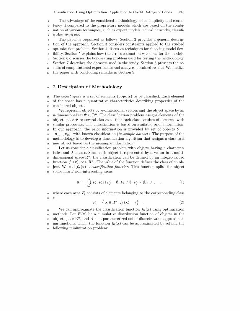
tics (see Figure 2). For small training sets, the model fits the data with zero20

in-sample error, whereas the expected out-of sample error is large. As the size21

of the training set increases, the expected in-sample error diverges from zero22

(the model cannot exactly fit the training data). Increasing the size of the23

training set leads to a larger expected in-sample error and a smaller expected24

out-of-sample error. For sufficiently large datasets, the in-sample and out-of-25

sample errors are quite close. In this case, we say that the model is saturated26

with data.27

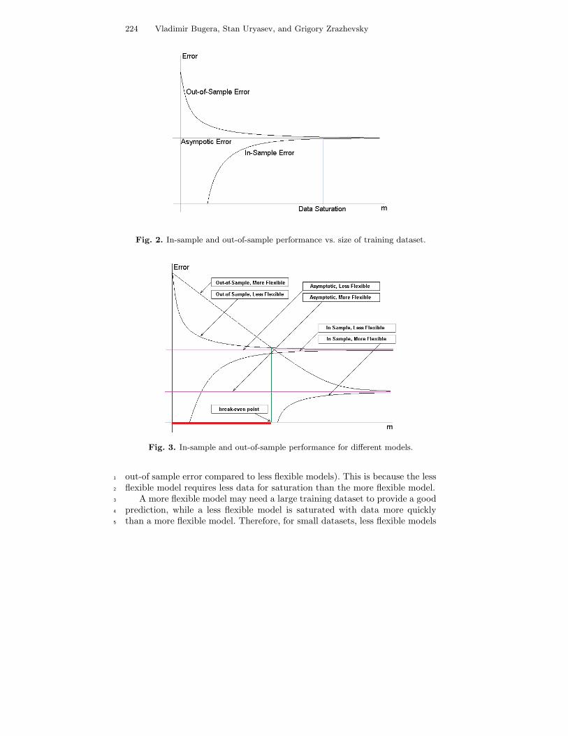
We say that the class of models A is more flexible than the class of models B28

if the class A includes the class B. Imposing constraints reduces the flexibility29

of the model. Figure 3 illustrates theoretical in/out-of-sample characteristics30

for two classes of models with different flexibilities. For small training sets,31

the less flexible model gives a smaller expected out-of-sample error (compared32

to the more flexible model) and, consequently, predicts better than the more33

flexible model. However, the more flexible models outperform the less flexible34

models for large training sets (more flexible models have a smaller expected35


Fig. 2. In-sample and out-of-sample performance vs. size of training dataset.

Fig. 3. In-sample and out-of-sample performance for different models.

out-of sample error compared to less flexible models). This is because the less1

flexible model requires less data for saturation than the more flexible model.2

A more flexible model may need a large training dataset to provide a good3

prediction, while a less flexible model is saturated with data more quickly4

than a more flexible model. Therefore, for small datasets, less flexible models5


tend to outperform (out-of sample) more flexible models. However, for large1

datasets, more flexible models outperform (out-of-sample) less flexible ones.2

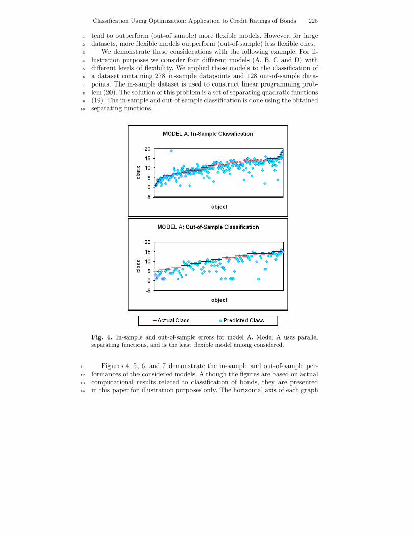
We demonstrate these considerations with the following example. For il-3

lustration purposes we consider four different models (A, B, C and D) with4

different levels of flexibility. We applied these models to the classification of5

a dataset containing 278 in-sample datapoints and 128 out-of-sample data-6

points. The in-sample dataset is used to construct linear programming prob-7

lem (20). The solution of this problem is a set of separating quadratic functions8

(19). The in-sample and out-of-sample classification is done using the obtained9

separating functions.10

Fig. 4. In-sample and out-of-sample errors for model A. Model A uses parallelseparating functions, and is the least flexible model among considered.

Figures 4, 5, 6, and 7 demonstrate the in-sample and out-of-sample per-11

formances of the considered models. Although the figures are based on actual12

computational results related to classification of bonds, they are presented13

in this paper for illustration purposes only. The horizontal axis of each graph14


Fig. 5. In-sample and out-of-sample errors for model B. Model B uses separatingfunctions without any constraints, and is the most flexible model. It has the bestin-sample performance than Model A, but fails to assign classes for most of out-of-sample objects.

corresponds to the object number, which is ordered according to the object ac-1

tual class number. The vertical line corresponds to the calculated by the model2

class number. The solid line on the graph represents the actual class number3

of an object. The round-point line represents the calculated class. The left4

graphs show in-sample classification: the class is computed by the separating5

functions for the objects from the in-sample dataset. The right graphs show6

out-of-sample classification: the class is computed by the separating functions7

for the objects from the out-of-sample dataset.8

Model A uses “parallel” quadratic separating functions. This case corre-9

sponds to the classification model considered by Bugera et al. (2003), where10

instead of multiple separating functions one utility function was used. The11

classification with the utility function can be interpreted as a classification12

with separating functions (15) with the following constraints on the functions13


Fig. 6. In-sample and out-of-sample errors for model C. Model C is obtained fromModel B by imposing feasibility constraints. This makes the out-of-sample predictionpossible for all out-of-sample objects.

Uα (x) =n∑

i=1

n∑j=1

aαijxixj +

n∑i=1

bαi xi + cα:1

∀α1, α2 ∈ {0, .., J} : ∀i, j ∈ {0, .., n} : aα1ij = aα2

ij , bα1i = bα2

i (39)

Constraints (39) make the separating functions parallel in the sense that2

the difference between the functions remains the same for all the points of the3

object space.4

Figure 4 shows that Model A has large errors for both in-sample and5

out-of-sample calculations. According to Figure 8, when a model has approx-6

imately the same in-sample and out-of-sample errors, the data saturation oc-7

curs. Therefore, the out-of-sample performance cannot be improved by reduc-8

ing flexibility of the model. A more flexible model should be considered.9

Model B uses quadratic separating functions without any constraints. This10

model is more flexible than Model A, because it has more control variables.11


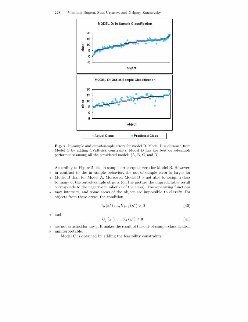
Fig. 7. In-sample and out-of-sample errors for model D. Model D is obtained fromModel C by adding CVaR-risk constraints. Model D has the best out-of-sampleperformance among all the considered models (A, B, C, and D).

According to Figure 5, the in-sample error equals zero for Model B. However,1

in contrast to the in-sample behavior, the out-of-sample error is larger for2

Model B than for Model A. Moreover, Model B is not able to assign a class3

to many of the out-of-sample objects (on the picture the unpredictable result4

corresponds to the negative number -1 of the class). The separating functions5

may intersect, and some areas of the object are impossible to classify. For6

objects from these areas, the condition7

U0 (x∗) , ..., Uj−1 (x∗) > 0 (40)

and8

Uj (x∗) , ..., UJ (x∗) ≤ 0 (41)

are not satisfied for any j. It makes the result of the out-of-sample classification9

uninterpretable.10

Model C is obtained by adding the feasibility constraints11


Fig. 8. Nature of risk constraint. For an optimal solution of the optimization prob-lem with the CVaR constraints, the α-CVaR largest of the jth class (the average ofUj(x) for the largest α% of objects from the jth class) is smaller at least by δ thanthe α-CVaR smallest of the (j + 1)th class (the average of Uj+1(x) for the smallestα% of objects from the (j + 1)th class).

Uj−1(xi) ≤ Uj(xi), j ∈ {1, .., J} , i = 1, ..,m . (42)

to Model B. Since Model C is less flexible then Model B, the in-sample error1

becomes greater than in Model B (see Figure 6). On the other hand, the model2

has a better out-of-sample performance than Models A and B. Moreover, a3

feasibility constraint makes the classification possible for any out-of-sample4

object. Since there is a significant discrepancy between in-sample and out-of-5

sample performances of the model, it is reasonable to impose more constraints6

on the model.7

Model D is obtained by adding CVaR-risk constraints to Model C:8

230 Vladimir Bugera, Stan Uryasev, and Grigory Zrazhevsky{ς+j + 1

α1Ij

∑x∈Xj

(Uj(x)− ς+

j

)+

}≤{

−ς−j+1 − 1α

1Ij+1

∑x∈Xj+1

(−Uj(x)− ς−j+1

)+

}− δ

j = 1, .., I − 1. (43)

Figure 7 shows that this model has higher in-sample error compared to1

Model B, but the out-of-sample performance is the best among the considered2

models. Moreover, the risk constraint reduces the number of many-class mis-3

classification jumps. Whereas Model C has 8 out-of-sample objects for which4

the value of misprediction is more than 5 classes, Model D has only one object5

with a 5-class misprediction. So, Model D has the best out-of-sample perfor-6

mance among all the considered models. This has been achieved by choosing7

appropriate flexibility of the model.8

A model with low flexibility may fit an in-sample dataset well. For models9

with a high in-sample error (such as Model A), more flexibility can be added10

by introducing more control variables to the model. In classification models11

with separating functions, feasibility constraints play a crucial role because12

they make classification always possible for out-of-sample objects. An exces-13

sive flexibility of the model may lead to “overfitting” and poor prediction14

characteristics of the model. To remove excessive flexibility of the considered15

models various types of constraints (such as risk constraints) can be imposed.16

The choice of the types of constraints, as well as the choice of the class of17

separating functions, plays a critical role for good out-of-sample performance18

of the algorithm.19

5 Error Estimation20

To estimate the performance of the considered models, we use the “leave-one-21

out” cross validation scheme. For the description of this scheme and other cross22

validation approaches, see, for instance, Efron and Tibshirani (1994). Let us23

denote by m a number of objects in the considered dataset. For each model24

(defined by the classes of the constraints imposed on optimization problem25

(20)), we performed m experiments. By excluding objects xi one by one from26

the set X , we constructed m training sets,27

Yi = X\{xi}

, i = 1, ..,m .

For each set Yi, we solved (20) optimization problems with the appropriate28

set of constraints and found the optimal parameters of the separating func-29

tions {Uα0 (x) , .., UαJ (x)}. Further, we computed the number of misclassified30

objects Mi from the set Yi. Let us introduce the variable31

Pi ={

0, if {Uα0 (x) , .., UαJ (x)} correctly classifies xi,1, otherwise .

(44)


The in-sample error estimate Ein−sample is calculated by the following1

formula:2

Ein−sample =1m

m∑i=1

Mi

(m− 1)=

1m (m− 1)

m∑i=1

Mi, (45)

where Mi is the number of misclassified objects in the set Yi. In the last for-3

mula, the ratio Mi

m−1 estimates the probability of an in-sample misclassification4

in the set Yi. We calculated the average of these probabilities to estimate the5

in-sample error.6

The out-of-sample error estimate Eout−of−samle is defined by the ratio of7

the total number of the misclassified out-of-sample objects in m experiments8

to the number of experiments:9

Eout−of−sample =1m

m∑i=1

Pi . (46)

The considered leave-one-out cross-validation scheme provides the highest10

confidence level (by increasing the number of experiments) while effectively11

improving the predicting power of the model (by increasing the size of the12

in-sample datasets)13

6 Bond Classification Problem14

We have tested the approach with a bond classification problem. Bonds repre-15

sent the most liquid class of the fixed-income securities. A bond is an obligation16

of the bond issuer to pay cash flow to the bond holder according to the rules17

specified at the time the bond is issued. A bond pays a specific cash flow (face18

value) at the time of maturity. In addition, a bond may pay periodic coupon19

payments.20

Although a bond generates a prespecified cash flow stream, it may default,21

if an issuer gets into financial difficulties or becomes a bankrupt. To charac-22

terize this risk, bonds are rated by several rating organizations (Standard &23

Poor’s and Moody’s are major rating companies). Bond rating evaluates the24

possibility of default of a bond issuer based on the issuer’s financial condition25

and profits potential. The assignment of a rating class is mostly based on the26

issuer’s financial status. A rating organization evaluates the status using ex-27

pert opinions and formal models based on various factors including financial28

ratios, such as the ratio of debt to equity, the ratio of current assets to current29

liabilities, and the ratio of cash flow to outstanding debt.30

According to Standard and Poor’s, bond ratings start at AAA for bonds31

having the highest investment quality, and end at D for bonds in payment32

default. The rating may be modified by a plus or minus to show relative33

standing within the category. Typically, a bond with a lower rating has a34

lower price than a bond generating the same cash flow, but having a higher35

rating.36


In this study, we have replicated Standard & Poor’s ratings of bonds using1

the suggested classification methodology. The rating replication problem is2

reduced to a classification problem with 20 classes.3

7 Description of Data4

For the computational verification of the proposed methodology we used sev-5

eral datasets (A, W, X, Y, Z) provided by the research group of the RiskSolu-6

tions branch of Standard and Poor’s, Inc. The datasets contain quantitative7

information about several hundred companies rated by Standard and Poor’s,8

Inc. Each entry in the datasets has fourteen fields that correspond to certain9

parameters of a specific firm in a specific year. The first two fields are the com-10

pany name, and the year when the rating was calculated. We used these fields11

as identifiers of objects for classification. The next eleven fields contain quan-12

titative information about financial performance of the considered company.13

These fields are used for the decision-making in the classification process. The14

last field is the credit rating of the company assigned by Standard and Poor’s,15

Inc. Table 1 represents the information used for classification.16

Table 1. Data format of an entry of the dataset.

Identifier Quantitative characteristics Class

1) Company Name 1) Industry Sector 1) Credit rating2) Year 2) EBIT interests coverage (times)

3) EBITDA interest coverage (times)4) Return on capital (%)5) Operating income/sales (%)6) Free operating cash flow/total debt (%)7) Funds form operations/total debt (%)8) Total debt/capital (%)9) Sales (mil)10) Total equity (mil)11) Total assets (mil)

We preprocessed the data and rescaled all quantitative characteristics into17

[-1,1] intervals: all quantitative characteristics are monotonic. Since the total18

number of rating classes equals 20, we used integer numbers from 1 to 20 to19

represent the credit rating of an object. The rating is arranged according to20

credit quality of the objects: the greater value corresponds to the better credit21

rating.22

In the case study, we considered 5 different datasets (A, W, X, Y, Z) to23

verify the proposed methodology for different sizes of the input data. Each24

set was split into an in-sample set and an out-of-sample set. The first one was25


used for developing a model, and the second one was used for the verification1

of the out-of-sample performance of the developed model. Table 2 contains2

information about the sizes of the considered datasets.3

Table 2. Sizes of the considered datasets.

Dataset A W X Y Z

Size of Set 406 205 373 187 108Size of In-Sample 278 172 315 157 89Size of Out-of-Sample 128 33 58 30 19

8 Numerical Experiments4

For dataset A we performed computational experiments with 16 models gen-5

erated by all possible combinations of four different types of constraints. For6

each dataset W, X, Y, and Z we found a model with the best out-of-sample7

performance.8

For dataset A we applied optimization problem (20) with Feasibility Con-9

straints (F). Besides, we applied all possible combinations of the following four10

types of constraints: Gradient Monotonicity Constraints (GM), Monotonicity11

of Separation Function w.r.t. Class Constraints (MSF), Risk Constraints (R),12

and Level Squeezing Constraints (LSQ). Each combination of the constraints13

corresponds to one of 16 different models, see Table 3. Although we considered14

other types of constraints (see Section 3.3), we report the results only for the15

models with F-, GM-, MSF-, R- and LSQ-constraints.16

The numerical experiments were conducted with Pentium III , 1.2GHz17

in C/C++ environment. The linear programming problems were solved by18

CPLEX 7.0 package. The calculation results for 16 models for dataset A are19

presented in Table 4 and Figure 9.20

Figure 9 represents in-sample and out-of-sample errors for different mod-21

els. For each model there are three columns representing the computational22

results. The first column corresponds to the percentage of in-sample classifica-23

tion error, the second column corresponds to the percentage of out-of-sample24

classification error, and the third column represents the average out-of-sample25

classification expressed in percents (100% misprediction corresponds to the26

case when the difference between actual and calculated classes equals 1).27

On Figure 9, the models are arranged according to an average of out-of-28

sample error (see Table 4, column AVR). Models 0000 and 0010 have zero in-29

sample error. These two models are the most “flexible” – they fit the data with30

zero objective in (20). The smallest average out-of-sample error is obtained31

by 0101- model with MSF and LSQ constraints. Table 4 shows that this32

model has the lowest maximal misprediction. Models 0100 and 0110 have the33


Table 3. List of the considered models.

Model IdentificatorTypes of Constraints AppliedGM MSF R LSQ

00000001 YES0010 YES0011 YES YES0100 YES0101 YES YES0110 YES YES0111 YES YES YES1000 YES1001 YES YES1010 YES YES1011 YES YES YES1100 YES YES1101 YES YES YES1110 YES YES YES1111 YES YES YES YES

Fig. 9. In-sample and out-of-sample errors for various models.

minimal number of out-of-sample mispredictions (column Error(1)), but the1

maximal mispredictions (column MAX) for these models are high. It is worth2

mentioning that imposing constraints on the separating functions increases3

the computing time. However, for all the considered optimization problems,4

the classification procedure did not take more than 5 minutes: The CPLEX5

LP solver, that was used for this study, computed classification model 11116

(all constraints were imposed) in about 5 minutes. Pentium III 1.2Ghz was7


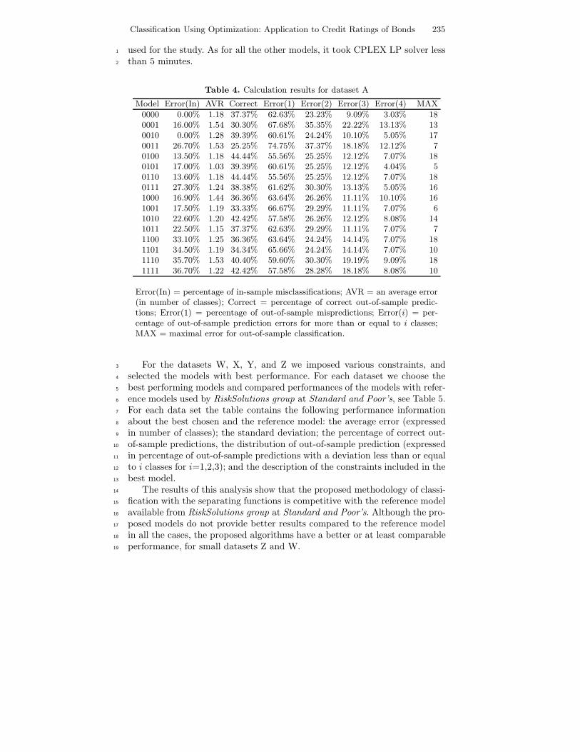
used for the study. As for all the other models, it took CPLEX LP solver less1

than 5 minutes.2

Table 4. Calculation results for dataset A

Model Error(In) AVR Correct Error(1) Error(2) Error(3) Error(4) MAX

0000 0.00% 1.18 37.37% 62.63% 23.23% 9.09% 3.03% 180001 16.00% 1.54 30.30% 67.68% 35.35% 22.22% 13.13% 130010 0.00% 1.28 39.39% 60.61% 24.24% 10.10% 5.05% 170011 26.70% 1.53 25.25% 74.75% 37.37% 18.18% 12.12% 70100 13.50% 1.18 44.44% 55.56% 25.25% 12.12% 7.07% 180101 17.00% 1.03 39.39% 60.61% 25.25% 12.12% 4.04% 50110 13.60% 1.18 44.44% 55.56% 25.25% 12.12% 7.07% 180111 27.30% 1.24 38.38% 61.62% 30.30% 13.13% 5.05% 161000 16.90% 1.44 36.36% 63.64% 26.26% 11.11% 10.10% 161001 17.50% 1.19 33.33% 66.67% 29.29% 11.11% 7.07% 61010 22.60% 1.20 42.42% 57.58% 26.26% 12.12% 8.08% 141011 22.50% 1.15 37.37% 62.63% 29.29% 11.11% 7.07% 71100 33.10% 1.25 36.36% 63.64% 24.24% 14.14% 7.07% 181101 34.50% 1.19 34.34% 65.66% 24.24% 14.14% 7.07% 101110 35.70% 1.53 40.40% 59.60% 30.30% 19.19% 9.09% 181111 36.70% 1.22 42.42% 57.58% 28.28% 18.18% 8.08% 10

Error(In) = percentage of in-sample misclassifications; AVR = an average error(in number of classes); Correct = percentage of correct out-of-sample predic-tions; Error(1) = percentage of out-of-sample mispredictions; Error(i) = per-centage of out-of-sample prediction errors for more than or equal to i classes;MAX = maximal error for out-of-sample classification.

For the datasets W, X, Y, and Z we imposed various constraints, and3

selected the models with best performance. For each dataset we choose the4

best performing models and compared performances of the models with refer-5

ence models used by RiskSolutions group at Standard and Poor’s, see Table 5.6

For each data set the table contains the following performance information7

about the best chosen and the reference model: the average error (expressed8

in number of classes); the standard deviation; the percentage of correct out-9

of-sample predictions, the distribution of out-of-sample prediction (expressed10

in percentage of out-of-sample predictions with a deviation less than or equal11

to i classes for i=1,2,3); and the description of the constraints included in the12

best model.13

The results of this analysis show that the proposed methodology of classi-14

fication with the separating functions is competitive with the reference model15

available from RiskSolutions group at Standard and Poor’s. Although the pro-16

posed models do not provide better results compared to the reference model17

in all the cases, the proposed algorithms have a better or at least comparable18

performance, for small datasets Z and W.19


Table 5. Comparison of best found model with reference model for sets W, X, Yand Z.

Model W X Y Z

In-Sample 172 315 157 89Out-of-Sample 33 58 30 19

Model Best Refer. Best Refer. Best Refer. Best Refer.

AVR 1.82 1.18 1.67 1.02 1.93 1.13 2.21 2.32STDV 1.72 0.92 2.45 1.07 2.60 1.50 2.20 2.50Correct 33.3% 21.2% 24.1% 37.9% 30.0% 50.0% 15.8% 21.1%1-Class area 42.4% 72.7% 53.4% 70.7% 60.0% 70.0% 42.1% 63.2%2-Class area 69.7% 87.9% 86.2% 94.8% 80.0% 83.3% 78.9% 68.4%3-Class area 84.8% 100.0% 94.8% 96.6% 86.7% 86.7% 84.2% 68.4%4-Class area 93.9% 100.0% 96.6% 98.3% 86.7% 96.7% 84.2% 78.9%

ConstraintsFeasibility Feasibility Feasibility Feasibility

MSF MSF MSF CVaR MSF

For each dataset the table has two columns. The first column corresponds to thebest found model; the second column corresponds to the reference model fromRiskSolutions. Each column contains information about out-of-sample perfor-mance of the corresponding model.AVR = an average error (in number of classes); STDV = a standard devia-tion; Correct = percentage of correct out-of-sample predictions; i-Class area =percentage of out-of-sample predictions with a deviation less than or equal to iclasses; Constraints = description of the constraints included in the best model

9 Concluding Remarks1

We extended the methodology discussed in previous work (Bugera et al., 2003)2

to the case of multi-class classification. The extended approach is based on3

finding “optimal” separating functions belonging to a prespecified class of4

functions. We have considered the models with quadratic separating func-5

tions (in indicator parameters) with different types of constraints. As before,6

selecting a proper class of constraints plays a crucial role in the success of the7

suggested methodology: by imposing constraints, we adjust the flexibility of8

a model to the size of the training dataset. The advantage of the considered9

methodology is that the optimal classification model can be found by linear10

programming techniques, which can be efficiently used for large datasets.11

We have applied the developed methodology to a bond rating problem. We12

have found that for the considered dataset, the best out-of-sample character-13

istics (the smallest out-of sample error) are delivered by the model with MSF14

and LSQ constraints on the control variables (coefficients of the separating15

function).16

The study was focused on the evaluation of computational characteristics17

of the suggested approach. As before, despite the fact that the obtained results18


are data specific, we conclude that the developed methodology is a robust1

classification technique suitable for a variety of engineering applications. The2

advantage of the proposed classification is its simplicity and consistency if3

compared to the proprietary models which are based on the combination of4

various techniques, such as expert models, neural networks, classification trees5

etc.6

References7

Bugera, V., Konno, H. and Uryasev, S.: 2003, Credit cards scoring with8

quadratic utility function, Journal of Multi-Criteria Decision Analysis9

11(4-5), 197–211.10

Efron, B. and Tibshirani, R.J.: 1994, An Introduction to the Bootstrap, Chap-11

man & Hall, New York.12

Konno, H., Gotoh, J. and Uho, T.: 2000, A cutting plane algorithm for semi-13

definite programming problems with applications to failure discrimination14

and cancer diagnosis, Working Paper 00-5, Tokyo Institute of Technology,15

Center for research in Advanced Financial Technology, Tokyo.16

Konno, H. and Kobayashi, H.: 2000, Failure discrimination and rating of17

enterprises by semi-definite programming, Asia-Pacific Financial Markets18

7, 261–273.19

Mangasarian, O., Street, W. and Wolberg, W.: 1995, Breast cancer diagnosis20

and prognosis via linear programming, Operations Research 43, 570–577.21

Pardalos, P.M., Michalopoulos, M. and Zopounidis, C.: 1997, On the use of22

multi-criteria methods for the evaluation of insurance companies in greece,23

in C. Zopounidis (ed.), New Operational Approaches for Financial Modeling,24

Physica, Berlin-Heidelberg, pp. 271–283.25

Rockafellar, R.T. and Uryasev, S.: 2000, Optimization of conditional value-26

at-risk, The Journal of Risk 2(3), 21–41.27

Rockafellar, R.T. and Uryasev, S.: 2002, Conditional value-at-risk for general28

loss distributions, Journal of Banking and Finance 26(7), 1443–1471.29

Rockafellar, R.T., Uryasev, S. and Zabarankin, M.: 2002, Generalized devia-30

tions in risk analysis, Finance and Stochastics 10, 51–74.31

Vapnik, V.: 1998, Statistical Learning Theory, John Wiley & Sons, New York.32

Zopounidis, C. and Doumpos, M.: 1997, Preference desegregation methodol-33

ogy in segmentation problems: The case of financial distress, in Zopouni-34

dis C. (ed.), New Operational Approaches for Financial Modeling, Physica,35

Berlin-Heidelberg, pp. 417–439.36

Zopounidis, C., Pardalos, P., Doumpos, M. and Mavridou, T.: 1998, Multicri-37

teria decision aid in credit cards assessment, in C. Zopounidis and P. Parda-38

los (eds), Managing in Uncertainty: Theory and Practice, Kluwer Academic39

Publishers, New York, pp. 163–178.40

classiﬁcation using optimization: application to …¬cation using optimization: application to...

Documents