classification and clustering problems in...

Classification and clustering problems in microarray analysis

and some recent advances

George C. TsengDept of Bioststistics / Human Genetics

University of Pittsburgh12/15/04

2004 Taipei Symposium on Statistical Genomics Outline1. Characteristics of microarray data

1. Dimension reduction: PCA, MDS2. Clustering

1. Intro. & issues in microarray2. Dissimilarity measure & filtering

• Correlation-based• Distance-based

3. Estimating # of clusters4. Methods & comparison

• Hierarchical, K-means, SOM, Tight clustering5. Common mistakes & discussion

3. Classification1. Intro. & issues in microarray2. Methods & comparison

• Linear & quadratic discriminant, CART, SVM 3. Gene (feature) selection

• Ranking, Recursive Feature Elimination (RFE)4. Cross validation & overfitting problem5. Common mistakes & discussion

Experimental designImage analysis

Normalization

Data matrix

row.names chromosome sample1 sample2 sample3 sample4time0 time3 time5 time7

96669_at 8.00 0.00 -0.10 0.02 -0.27100877_at 6.00 -0.22 0.59 0.20 0.4693490_at 15.00 0.00 0.02 -0.02 -0.07100978_at 8.00 -0.40 0.03 -0.18 -0.02103516_at 15.00 NA NA NA NA160378_at 19.00 0.16 0.41 0.76 0.5799670_at 19.00 -0.11 0.11 0.04 -0.1298569_at 2.00 NA 0.11 0.35 0.3793794_at 8.00 0.01 0.45 -0.02 0.12

samples

genes

10~500 samples

10K~30Kgenes

Experimental designImage analysis

Normalization

Identify differentially expressed genes

Data visualization Regulatory network

Clustering

Statistical issues in microarray analysis

Classification

1. High dimensional complex data structure

2. Gene dependencies.

3. High dimension and low sample size often happens.

4. Existence of outliers.

5. Sometimes comes with clinical data such as survival, malignancy status, and other covariates such as sex, age and smoking.

1. Characteristics of microarray data1.1 Dimension reduction

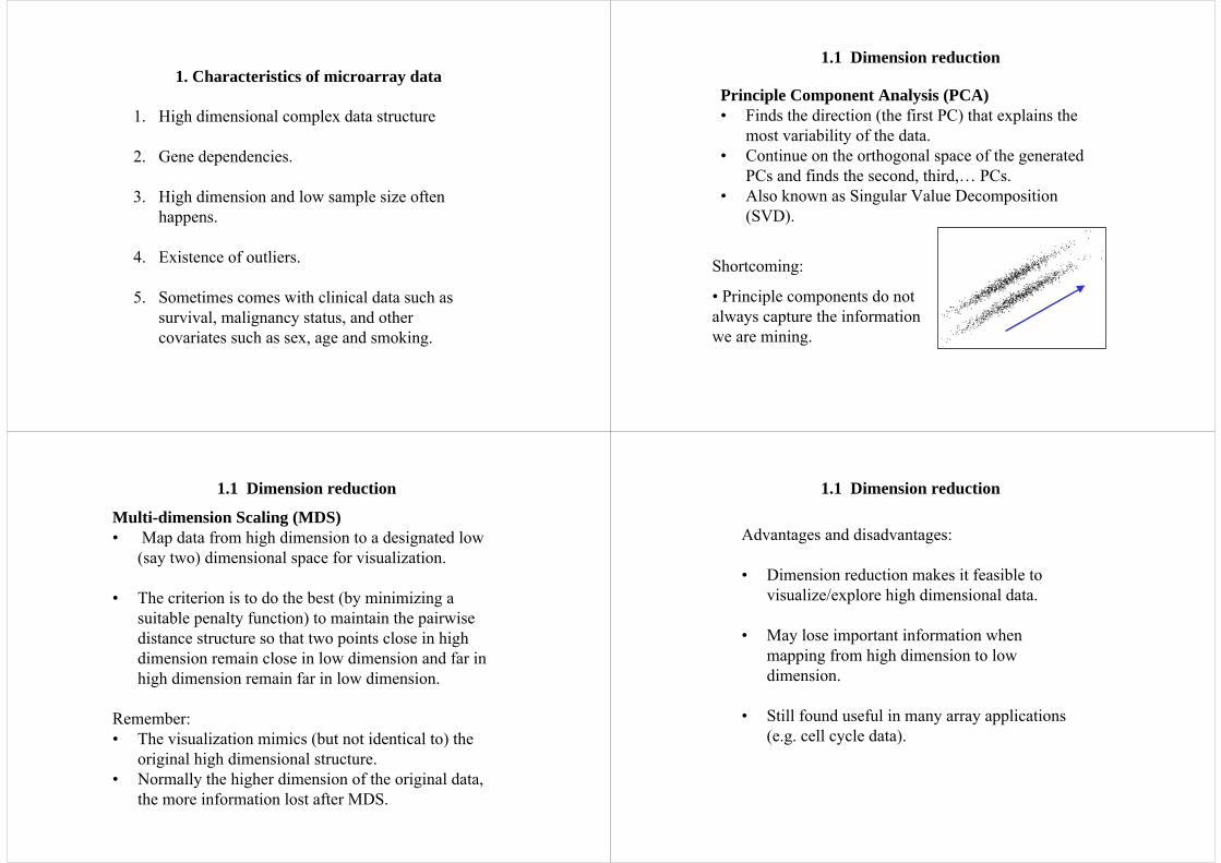
Principle Component Analysis (PCA)• Finds the direction (the first PC) that explains the

most variability of the data.• Continue on the orthogonal space of the generated

PCs and finds the second, third,… PCs.• Also known as Singular Value Decomposition

(SVD).

Shortcoming:

• Principle components do not always capture the information we are mining.

Multi-dimension Scaling (MDS)• Map data from high dimension to a designated low

(say two) dimensional space for visualization.

• The criterion is to do the best (by minimizing a suitable penalty function) to maintain the pairwise distance structure so that two points close in high dimension remain close in low dimension and far in high dimension remain far in low dimension.

Remember:• The visualization mimics (but not identical to) the

original high dimensional structure.• Normally the higher dimension of the original data,

the more information lost after MDS.

1.1 Dimension reduction

Advantages and disadvantages:

• Dimension reduction makes it feasible to visualize/explore high dimensional data.

• May lose important information when mapping from high dimension to low dimension.

• Still found useful in many array applications (e.g. cell cycle data).

1.1 Dimension reduction

2. Clustering

Goal: Given a dissimilarity measure, n points are grouped into k clusters based on their similarity.

General problems encountered:1. Which dissimilarity measure to use?2. How many # of clusters, k?3. How to assign the points into clusters?

Clustering genes : similar gene expression pattern may imply co-regulation/network.

Clustering samples: identify potential sub-classes of disease

More specific clustering problems in microarray:

1. Which dissimilarity measure to use?2. How many # of clusters, k?3. Gene selection (filtering)

• Filter genes before clustering genes.• Filter genes before clustering samples.

4. How to assign the points into clusters?5. Should we allow noise genes/samples not

being clustered?

2.1 Issues in microarray

2.2 Dissimilarity measure

Correlation-based:• Pearson correlation

• Uncentered correlation

• Absolute value of correlation(capture both positive and negative correlation)

Biologically notinteresting


Distance-based:• Euclidean

• City block (Mahattan)

Correlation

Euclidean distance


The procedure we normally use when clustering genes:Filter genes according to their coefficient of variation (CV).

Standardize gene rows to mean 0 stdev 1.

Use Euclidean distance.

Remark:• Step 1. takes into account the fact that high abundance

genes normally have larger variation. This filters “flat”genes.

• Step 2. make Euclidean distance and correlation equivalent.• Many useful methods require the data to be in Euclidean

space.

2.3 Estimating # of clustersMilligan & Cooper(1985) compared 30 published rules.1. Calinski & Harabasz (1974)

2. Hartigan (1975)

, Stop when H(k)<10

3. Tibshirani, Walther & Hastie (2000)

4. Tibshirani et al(2001), Dudoit & Fridlyand(2002)Prediction-based resampling approach.

)/()()1/()()(max

knkWkkBkCH−−

=

))(log()))((log()(max * kWkWEkGap nn −=

Estimating # of clusters is rarely successful in microarray, except for some cell cycle study.

2.4 Clustering methods

• Hierarchical clustering• K-means / K-memoids• Self-Organizing maps• Gaussian mixture model• CLICK• FUZZY• Bayesian model-based clustering• Tight clustering• Penalized and weighted K-means


Hierarchical clustering:


Elongated clustersSensitive to outliers

Compact clustersSensitive to outliers

In betweenLess sensitive to outliers

(Linkage for hierarchical clustering)


Procedures:Step 1: estimate the number of clusters, k.Step 2: minimize the within-cluster dispersion to the cluster

centers.

Note:1. Points should be in Euclidean space. 2. Optimization performed by iterative relocation

algorithms. Local minimum inevitable.3. k has to be correctly estimated.

∑∑= ∈

−=k

j Ciji

j

CxkW1

2)(

K-means

Problems:Local minimumDoes not allow scattered genesEstimation of # of clusters


Model-based clustering

Fraley and Raftery (1998) applied a Gaussian mixture model.

(1) EM algorithm to maximize the classification likelihood.

(2) Bayesian Information Criterion (BIC) for determining k and the complexity of the covariance matrix.


Tight clustering:(a re-sampling method)

x

y

0 1 2 3 4 5

01

23

4

x

x

subsample 1

x

y

0 1 2 3 4 5

01

23

4

x

x

subsample 2

x

y

0 1 2 3 4 5

01

23

4

x

x

judgement by subsample 1

x

y

0 1 2 3 4 5

01

23

4

x

x

judgement by subsample 2

x

y

0 1 2 3 4 5

01

23

4

whole data

11

1 2 3 4 5

6 7 8 9 10


Tight clustering:

For sequence k>k0,1. Identify sets of genes that are constantly

clustered together under sub-sample clustering judgment. Consider the top q sets for each k.

2. Stop when for (k, k+1), two sets are nearly identical. Take the set corresponding to (k+1) as a tight cluster. Remove the identified cluster from the data.

3. Set k0=k0-1. Continue the procedure to find the next tight cluster.

• Slower computation when data large

• Allow genes not being clustered; only produce tight clusters

• Ease the problem of accurate estimation of # of clusters

• Biologically more meaningful

Tight clustering

• Model selection usually difficult• Local minimum problem

• Flexibility on cluster structure• Rigorous statistical inference

Model-based clustering

• The algorithm very heuristic• Solution sub-optimal due to 2D

geometry restriction

• Clusters has interpretation on 2D geometry (more interpretable)

SOM

• Local minimum• Estimating # of clusters

• Simplified Gaussian mixture model• Normally get nice clusters

K-means

• Very vulnerable to outliers• Tree not unique; gene closer

not necessarily more similar• Hard to read when tree is big

• Intuitive algorithm• Good interpretability• Do not need to estimate # of

clusters

Hierarchical clustering

DisadvantageAdvantage


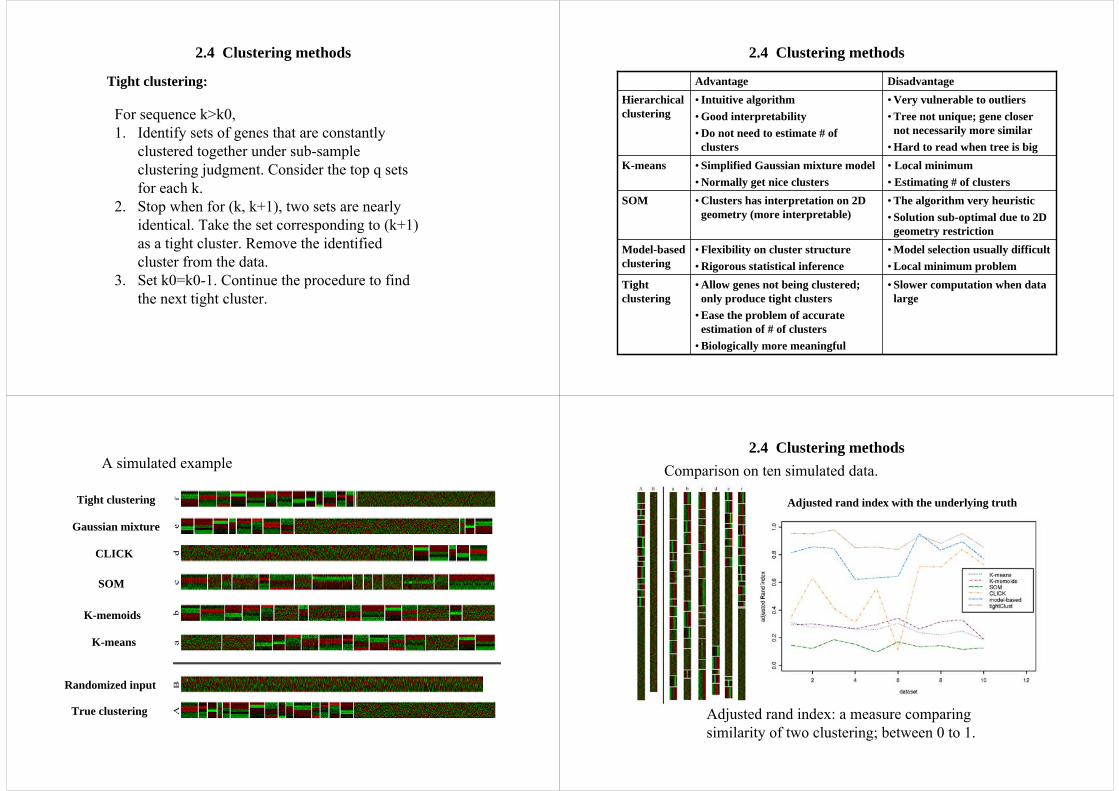
True clustering

Randomized input

K-means

K-memoids

SOM

CLICK

Gaussian mixture

Tight clustering

A simulated example

Adjusted rand index: a measure comparing similarity of two clustering; between 0 to 1.

2.4 Clustering methodsComparison on ten simulated data.

Adjusted rand index with the underlying truth

Things to keep in mind:

1. All clustering methods always returns a clustering result no matter how much information the data actually contains.

2. Thus clustering alone is only an exploratory, visualization and hypothesis generating tool, not a biological “proof”.

3. Watch out for mistakes with repeating data usage (overfitting) or tautology.

Hypothesis driven: hypothesis => experiments for validation.

Data driven: high-throughput experiment => data mining => generate further hypothesis => validation experiments

2.5 Common mistakes

Common mistakes or warnings:1. Run K-means with large k and get excited to

see patterns without further investigation.K-means can let you see patterns even in randomly generated data and besides human eyes tend to see “patterns”.

2. Identify genes that are predictive to survival (e.g. apply t-statistics to long and short survivors). Cluster samples based on the selected genes and find the samples are clustered according to survival status.

The gene selection procedure is already biased towards the result you desire.

2.5 Common mistakes

Common mistakes (con’d):3. Cluster samples into k groups. Perform F-test to

identify genes differentially expressed among subgroups.

Data has been re-used for both clustering and identifying differentially expressed genes. You always obtain a set of differentially expressed genes but not sure it’s real or by random.

2.5 Common mistakesReferences:

Clustering methods:• Hastie, T., Tibshirani, R. and Friedman, J. (2001). The elements of statistical

learning. Springer.• Yeung, K. Y., Fraley, C., Murua, A., Raftery, A. E. and Ruzzo, W. L. (2001).

Model-based clustering and data transformations for gene expression data.Bioinformatics 17, 977–987.

• Chipman, H., Hastie, T., Tibshirani, R. (2003) Clustering microarray data. Chapter 4 in Statistical Analysis of Gene Expression Microarray Data. Editor: Terry Speed. Chapman Hall/CRC.

• George C. Tseng and Wing H. Wong. (2004) Tight Clustering: A Resampling-based Approach for Identifying Stable and Tight Patterns in Data. Biometrics (in press)

• George C. Tseng. (2004) A Comparative Review of Gene Clustering in Expression Profile. in Proceedings of ICARCV 04' (to appear)

Reference:

Estimating # of clusters:•Tibshirani, Walther & Hastie (2000). Estimating the number of clusters in a dataset via the Gap statistic. Journal of the Royal Statistical Society, B, 63:411-423,2001•Dudoit, S. and Fridlyand, J. (2002). A prediction-based resampling method for estimating the number of clusters in a dataset. Genome Biology 3, 0036.1–21.•Milligan, G. W. and Cooper, M. C. (1985). An examination of procedures for determining the number of clusters in a data set. Psychometrika 50, 159–179.

3. Classification

Data: Objects {Xi, Yi}(i=1,…,n) i.i.d. from joint distribution {X, Y}. Each object Xi is associated with a class label Yi∈{1,…,K}.

Goal: Develop a classification rule that predicts the class label Y of a new observed object X.

Cross validation: Normally we divide data into training and testing. Use training data to learn the classification rule and testing data for evaluating classification error.

3.2 Methods

Bayes rule:For known class conditional densities pk(X)=f(X|Y=k), the Bayes rule predicts the class of an observation X by

C(X) = argmaxk p(k|x)

Specifically if pk(X)=f(X|Y=k)~N(µk, Σk),

∑=

lll

kkxp

xpxkp)(

)()|(π

π

C(x) = arg mink {(x- µk) Σk-1(x- µk)′ + log|Σk| - 2 log π k }

Linear Discriminant Analysis (LDA), DQDA, DLDA3.2 Methods

LDA: Σk = Σ ,C(x) = arg mink (µkΣ-1µk′ - 2x Σ-1µk′)

( )221,..., kGkk diag σσ=Σ :DQDA

∑ =⎪⎭

⎪⎬⎫

⎪⎩

⎪⎨⎧

+−

= Gg kg

kg

kggk

xxC 1

22

2log

)(minarg)( σ

σ

µ

( )221 ,..., Gk diag σσ=Σ :DLDA

∑ =⎪⎭

⎪⎬⎫

⎪⎩

⎪⎨⎧ −

= Gg

g

kggk

xxC 1 2

2)(minarg)(

σ

µ

(quadratic boundaries)

(linear boundaries)

(linear boundaries)

Linear Discriminant Analysis (LDA), DQDA, DLDA

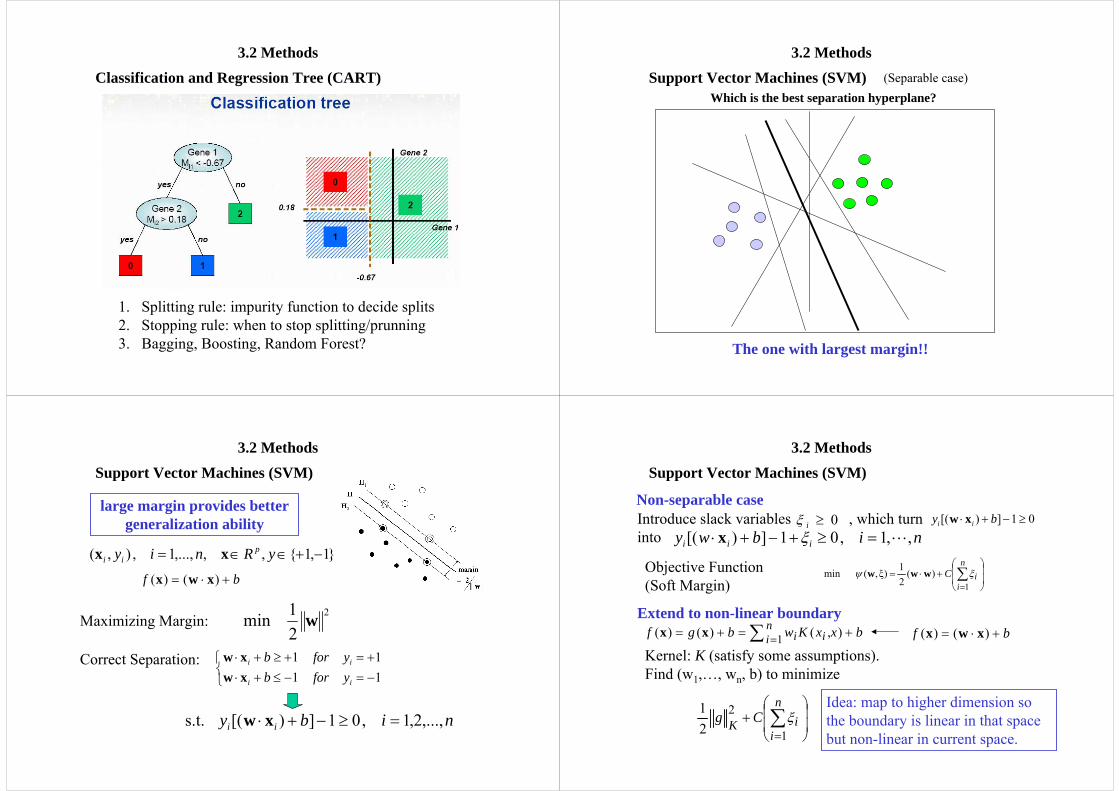
3.2 MethodsClassification and Regression Tree (CART)

1. Splitting rule: impurity function to decide splits2. Stopping rule: when to stop splitting/prunning3. Bagging, Boosting, Random Forest?

3.2 MethodsSupport Vector Machines (SVM) (Separable case)

The one with largest margin!!

Which is the best separation hyperplane?

2

21min w

niby ii ,...,2,1,01])[(s.t. =≥−+⋅xw

}1,1{,,,...,1,),( −+∈∈= yRniy pii xx

⎩⎨⎧

−=−≤+⋅+=+≥+⋅

1111

ii

ii

yforbyforb

xwxw

bf +⋅= )()( xwx

Maximizing Margin:

Correct Separation:

3.2 MethodsSupport Vector Machines (SVM)

large margin provides better generalization ability


Introduce slack variables , which turn into

0≥iξ 01])[( ≥−+⋅ by ii xwnibwy iii ,,1,01])[( L=≥+−+⋅ ξx

⎟⎟

⎠

⎞

⎜⎜

⎝

⎛+⋅= ∑

=

n

iiC

1)(

21)ξ,(min ξψ wwwObjective Function

(Soft Margin)

Non-separable case

Extend to non-linear boundarybf +⋅= )()( xwxbxxKwbgf n

i ii +=+= ∑ = ),()()( 1xx

Kernel: K (satisfy some assumptions).Find (w1,…, wn, b) to minimize

⎟⎟

⎠

⎞

⎜⎜

⎝

⎛+ ∑

=

n

iiK Cg

1

221 ξ

Idea: map to higher dimension so the boundary is linear in that space but non-linear in current space.


3.3 Gene Selection

Why gene selection?• Many genes are redundant and will introduce

noise that lower performance.

Filter methods:• Rank scores such as correlation, t-statistics, F-

statistics to select a desired number of genes.

Wrapper methods:• Iterative approach to identify the best set of genes

based on performance.• Forward selection, Backward selection, Forward-

backward selection.• The problem is similar to model selection in linear

regression.

3.3 Gene Selection

Filter methods is easy and fast but it has disadvantages: 1. Redundancy of features. Genes are dependent but the

method considers them independent.2. Interactions among genes can not be facilitated in this

method.

Wrapper methods tries to solve the problem but it’s 1. Slow and impossible to exhaust all searches.2. Easy to overfit.

e.g. Recursive Feature Elimination (RFE) is a back-ward selection wrapper method.

3.3 Gene SelectionRecursive Feature Elimination (RFE)

1. Train the classifier with SVM.

2. Compute the ranking criterion for all features (wi2 in

this case).

3. Remove the feature with the smallest ranking criterion.

4. Repeat step 1~3.

Note: The speed can be further improved by removing multiple features in each iteration.

An R package to implement RFE-SVM.http://www.hds.utc.fr/~ambroise/softwares/RFE/

3.3 Gene Selection

Recursive Feature Elimination (RFE)

Dashed lines: filter method by naïve rankingSolid lines: RFE (a wrapper method)

Guyon et al 2002

• 22 normal 40 Colon cancer tissues

• 2000 genes after pre-processing

• Leave-one-out cross validation

3.4 Overfitting

Overfitting problems:

The classification rule developed overfits to the training data and become not generalizable to the testing data.

e.g. • In CART, we can always develop a tree that

produces 0 classification error rate in training data. But applying this tree to the testing data will find large error rate (not generalizable)

Things to be aware:• Pruning the trees (CART)• Feature space (CART and non-linear SVM)

3.5 Common Mistakes

Common mistakes:1. Perform t-statistics to select a set of genes

distinguishing two classes. Restrict on this set of genes and apply do cross validation on a classification method to evaluate the classification error.

The selection of the genes should not apply the whole data if we want to evaluate the “true” classification error. The selection of genes already used information in testing data.

Common mistakes (cont’d):2. Suppose a rare (1%) subclass of cancer is to be

predicted. We take 50 rare cancer samples and 50 common cancer samples and find 0/50 errors in rare cancer and 10/50 for common cancer. => conclude 10% error rate!

The assessment of classification error rate should take population proportions into account. The overall error rate in this example is actually ~20%. In this case, it’s better to specify specificity and sensitivity separately.

3.5 Common Mistakes

References:

Classification methods:• Hastie, Tibshirani, Friedman “The Elements of Statistical Learning”, Springer,

2001.

• Speed (editor) “Statistical Analysis of Gene Expression Microarray Data”. Chapman & Hall/CRC, 2003

• N. Cristianini and J. Shawe-Taylor (2000) AN INTRODUCTION TO SUPPORT VECTOR MACHINES. Cambridge University Press

• Dudoit, et al, :Comparison of discrimination methods for the classification of tumors using gene expression data, JASA, 2002

Gene (feature) selection:• Guyon, I., Weston, J., Barnhill, S., & Vapnik, V. (2002) Gene Selection for

Cancer Classification using Support Vector Machines Mach. Learn. 46, 389-422

Clustering:• Clustering is a powerful exploratory tool but does not

provide ultimate biological conclusion.• Exact estimation of # of clusters is usually impossible.• Recent new methods are developed specifically for

microarray and biological needs.

Topics not touched in the talk:• Incorporation of biological info. in clustering.• Bi-clustering.• Stability of clusters

Conclusion

Classification:• Classification is probably the analysis most relevant to

clinical application.• Interpretability and performance should be considered

when choosing among different methods

Topics not touched in the talk:• Incorporation of clinical data in the analysis• Resampling methods to improve classification:

Bagging, random forest,…

Conclusion

classification and clustering problems in...

Documents