1

Classifying Land Use/Land Cover in ArcGIS Prepared by Thomas J. Ballatore, Ph.D. Director, Lake Basin Action Network (LBAN) Affiliated Scientist, Center for Ecological Research, Kyoto University Visiting Researcher, International Lake Environment Committee (ILEC) Foundation Please send questions and comments to ballatore@lakebasin.org

Purpose of this Tutorial The purpose of this tutorial is to show you how to download Landsat images, how to prepare them in ArcGIS and how to use them in classifying land use/land cover. I use the case of Mt. Elgon on the Kenya/Uganda border.

Note Landsat images can be *very* large! In general, I download them as explained below. Perhaps you can do this, too, or perhaps your institution might have another way of accessing them. Nevertheless, getting your hands on the data itself can be one of the greatest hurdles for those without a fast Internet connection.

Selecting and Downloading the Landsat Images In this example, I introduce the use of Landsat images for land cover classification. Landsat has been active since 1972 and provides a completely free archive of images acquired from 1972-present from the various Landsat sensors. For Landsat downloads, I prefer to use the USGS Global Visualization Viewer website at: http://glovis.usgs.gov/ There are several ways to navigate to the images for your area of interest. I prefer to just click on the locator map (upper left, as shown below) as close as I can to the target area, in this case, Mt Elgon. After clicking, you should get the following pop-up window called the USGS Global Visualization Viewer. Please be aware that many internet browsers will automatically block this pop-up window from opening. Additionally, the pop-up usually requires a recent version of Java to be installed on your machine. When trying this out on a new computer, I sometimes use 2 or even 3 different browsers just to get it to work. Be patient! Once you get the pop-up (see below) to display, you will have access to an incredible archive of images that is worth any trouble at this point.

2

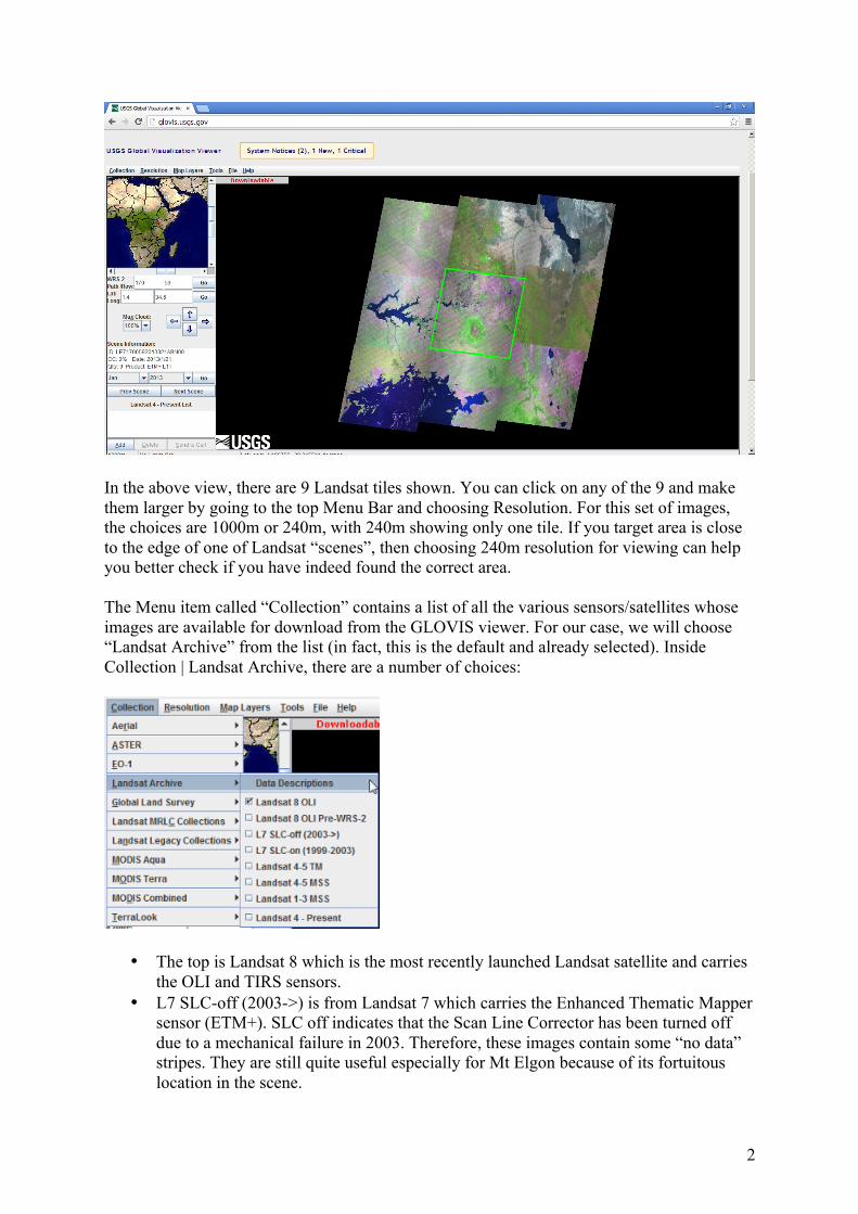
In the above view, there are 9 Landsat tiles shown. You can click on any of the 9 and make them larger by going to the top Menu Bar and choosing Resolution. For this set of images, the choices are 1000m or 240m, with 240m showing only one tile. If you target area is close to the edge of one of Landsat “scenes”, then choosing 240m resolution for viewing can help you better check if you have indeed found the correct area. The Menu item called “Collection” contains a list of all the various sensors/satellites whose images are available for download from the GLOVIS viewer. For our case, we will choose “Landsat Archive” from the list (in fact, this is the default and already selected). Inside Collection | Landsat Archive, there are a number of choices:

• The top is Landsat 8 which is the most recently launched Landsat satellite and carries the OLI and TIRS sensors.

• L7 SLC-off (2003->) is from Landsat 7 which carries the Enhanced Thematic Mapper sensor (ETM+). SLC off indicates that the Scan Line Corrector has been turned off due to a mechanical failure in 2003. Therefore, these images contain some “no data” stripes. They are still quite useful especially for Mt Elgon because of its fortuitous location in the scene.

3

• The L7 SLC-on (1999-2003) archive is for the images from Landsat 7’s ETM+ did

not have this mechanical problem.

• Landsat TM 4-5 TM is for the “thematic mapper” sensor on Landsat satellites 4 and 5, the later which is still operating without problem.

• Landsat TM 4-5 MSS is for the “Multispectral Scanner” sensor on Landsat satellites 4

and 5, the later which is still operating without problem.

• Landsat MSS 1-3 is the original MSS sensor on the Landsat satellites numbers 1-3, the former which started recording images in 1972.

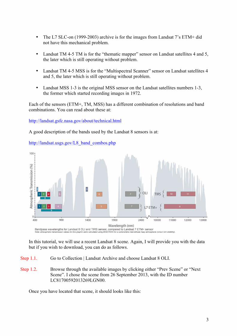
Each of the sensors (ETM+, TM, MSS) has a different combination of resolutions and band combinations. You can read about these at: http://landsat.gsfc.nasa.gov/about/technical.html A good description of the bands used by the Landsat 8 sensors is at: http://landsat.usgs.gov/L8_band_combos.php

In this tutorial, we will use a recent Landsat 8 scene. Again, I will provide you with the data but if you wish to download, you can do as follows.

Step 1.1. Go to Collection | Landsat Archive and choose Landsat 8 OLI.

Step 1.2. Browse through the available images by clicking either “Prev Scene” or “Next Scene”. I chose the scene from 26 September 2013, with the ID number LC81700592013269LGN00.

Once you have located that scene, it should looks like this:

4

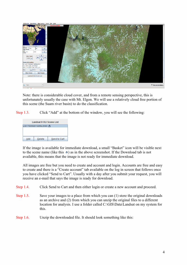
Note: there is considerable cloud cover, and from a remote sensing perspective, this is unfortunately usually the case with Mt. Elgon. We will use a relatively cloud free portion of this scene (the Suam river basin) to do the classification.

Step 1.3. Click “Add” at the bottom of the window, you will see the following:

If the image is available for immediate download, a small “Basket” icon will be visible next to the scene name (like this ) as in the above screenshot. If the Download tab is not available, this means that the image is not ready for immediate download. All images are free but you need to create and account and login. Accounts are free and easy to create and there is a “Create account” tab available on the log in screen that follows once you have clicked “Send to Cart”. Usually with a day after you submit your request, you will receive an e-mail that says the image is ready for download.

Step 1.4. Click Send to Cart and then either login or create a new account and proceed.

Step 1.5. Save your images to a place from which you can (1) store the original downloads as an archive and (2) from which you can unzip the original files to a different location for analysis. I use a folder called C:\GIS\Data\Landsat on my system for this.

Step 1.6. Unzip the downloaded file. It should look something like this:

5

The eleven Landsat 8 “bands” are distinguished by the last 2~3 characters of the tile name: B1 is Band 1 (0.45-0.52 um), and so on (see the table below). These TIF files are in GeoTIFF format which means they contain geographic coordinate information and do not need to be projected by you. For this Landsat scene, the projection is UTM53N, which is stated in “L5109036_03619960714_MTL.txt”. You will note that all bands except 8 have an unzipped file size of 107 MB. They have a spatial resolution of 30 meters. Bands 10 and 11 represent thermal radiation and have an original spatial resolution of 100m which is resampled to 30 for ease of use. Note there is a panchromatic band (Band 8) with spatial resolution of 15 m and a very large file size of around 428 MB! Band Spatial

Resolution (m) Spectral

Resolution (µm) Band 1 - Coastal/Aerosol 30 0.433 - 0.453 Band 2 - Blue 30 0.450 - 0.515 Band 3 - Green 30 0.525 - 0.600 Band 4 - Red 30 0.630 - 0.680 Band 5 - Near Infrared 30 0.845 - 0.885 Band 6 - Short Wavelength Infrared 30 1.560 - 1.660 Band 7 - Short Wavelength Infrared 30 2.100 - 2.300 Band 8 - Panchromatic 15 0.500 - 0.680 Band 9 - Cirrus 30 1.360 - 1.390 Band 10 - Long Wavelength Infrared 100 (resampled to 30) 10.30 - 11.30 Band 11 - Long Wavelength Infrared 100 (resampled to 30) 11.50 - 12.50

Supervised Classification There are two major approaches to classifying the pixels in a multiband raster: supervised and unsupervised classification. Despite the latter’s name, both require substantial input from the analyst. There is no such thing as automated classification! It is a laborious process and the result reflects the amount of effort put in as well as the quality of the groundtruth data against which a classification is judged. To keep the work to a reasonable time frame, I have trimmed the downloaded image so that only pixels from the Suam river basin are provided. You can get these files from the network.

6

Step 2.1. Copy the folder LC81700592013109LGN01 from the network location to your

computer inside C:\MtElgon\LULC. This contains the 11 Landsat 8 bands clipped to the Suam river basin area.

Step 2.2. Open a new map and save it as MtElgon_LULC.mxd.

Step 2.3. Add the 11 bands to the new map.

Step 2.4. In ArcToolbox, choose Data Management Tools | Projections and Transformations | Features | Project and execute the tool with the following information:

Step 2.5. In the ArcToolbox, go to Data Management Tools | Raster | Raster Processing | Composite Bands. Execute this tool with the following information:

Note that band 8 is not included and that bands 10 and 11 are hard to see in the above dialog.

7

Step 2.6. Double click on the new layer, and go to Properties and change the RGB composite settings to the following. This will give us a Color Infrared image commonly used in vegetation studies.

You should see something like this:

The next steps will be to use the Image Classification toolbar to define “training areas” and to carry out the supervised classification. This is a highly visual, iterative process that will be shown in a future screencast.