Classroom Notes

Mechanical Modeling of Muscles at a Glance

L. TeresiLaMS - Modeling & Simulation Lab

Universita degli Studi Roma Tre

February 3, 2011

z z z

A companion to the Series of Lectures on

Mathematical Models in Cardiac Physiology

Dip. di Matematica e Fisica “Niccolo Tartaglia”

Universita Cattolica del Sacro Cuore Brescia,

January 31 - February 2, 2011.

z z z

1

Contents

1 Key Words 3

2 Mechanical Muscles Modeling 42.1 Force and Velocity . . . . . . . . . . . . . . . . . . . . . . . . . . . . . . . . . . . 42.2 Muscle as a Black Box . . . . . . . . . . . . . . . . . . . . . . . . . . . . . . . . . 52.3 Gym session . . . . . . . . . . . . . . . . . . . . . . . . . . . . . . . . . . . . . . . 5

3 Hill’s equation for tetanized muscle 63.1 Isometric force-length relationship . . . . . . . . . . . . . . . . . . . . . . . . . . 8

4 Hill’s three-element model 94.1 Gym session . . . . . . . . . . . . . . . . . . . . . . . . . . . . . . . . . . . . . . . 10

5 Active tension 125.1 Physiology . . . . . . . . . . . . . . . . . . . . . . . . . . . . . . . . . . . . . . . . 125.2 State variables . . . . . . . . . . . . . . . . . . . . . . . . . . . . . . . . . . . . . 135.3 Evolution equations for physiological varibles . . . . . . . . . . . . . . . . . . . . 14

6 Mechanics in a Page! 15

7 Active Contraction: 1D setting 167.1 State variables . . . . . . . . . . . . . . . . . . . . . . . . . . . . . . . . . . . . . 167.2 Power . . . . . . . . . . . . . . . . . . . . . . . . . . . . . . . . . . . . . . . . . . 177.3 Constitutive recipes . . . . . . . . . . . . . . . . . . . . . . . . . . . . . . . . . . 177.4 Gym session . . . . . . . . . . . . . . . . . . . . . . . . . . . . . . . . . . . . . . . 19

8 Active Contraction: 3D setting 20

9 Kinematics 209.1 Motion . . . . . . . . . . . . . . . . . . . . . . . . . . . . . . . . . . . . . . . . . . 209.2 Anisotropic distortions . . . . . . . . . . . . . . . . . . . . . . . . . . . . . . . . . 219.3 Elastic Deformation . . . . . . . . . . . . . . . . . . . . . . . . . . . . . . . . . . 22

10 Elastic Energy 22

11 Attach-detach-contract model (release 2.8) 2511.1 State variables . . . . . . . . . . . . . . . . . . . . . . . . . . . . . . . . . . . . . 2511.2 Power . . . . . . . . . . . . . . . . . . . . . . . . . . . . . . . . . . . . . . . . . . 2611.3 Constitutive recipes . . . . . . . . . . . . . . . . . . . . . . . . . . . . . . . . . . 2611.4 Evolution equations. . . . . . . . . . . . . . . . . . . . . . . . . . . . . . . . . . . 27

2

1 Key Words

Mechanics and muscle physiology share many key words with quite different meanings; here westate our usage of some key terms.

• A muscle is active when, under the appropriate electro-chemical stimuli, it shortens and/or,exerts a force.

• A muscle shortens when, unloaded and unconstrained, is activated.

• Contraction is somehow used as synonymous of activation, an electro-chemical notion, orof shortening, a kinematical one. Beware of its meaning.

• A twitch is a single electro-chemical stimulus to a muscle, usually lasting a tenth of asecond or less. An appropriate sequence of twitches activates a skeletal muscle, a singletwitch is necessary for heart muscle.

• The adjectives rest or ground always refer to mechanics: they label a state at zero elasticenergy. Activation changes the ground state of muscles.

• The slack length is the length to which a non active muscle will return when unloaded; neverconfuse slack with ground length: they coincide when muscle is unloaded and inactive.Slack is used for a whole muscle, or for its subunits. A sarcomere slack length is ∼ 2.1µm.

• During an isometric exercise a muscle stays at fixed length; when activated, the muscleexerts a force against its constraints. Beware that in gym or physiological jargon, you mayhear of ‘isometric contraction’, a misleading expression in our context: here contractiondoes not have any kinematical significance.

• During an isotonic exercise a muscle is subject to a fixed load; when activated, it shortens(provided the load is below a given threshold).

• During an auxotonic exercise a muscle has to deal mostly with inertia forces, that maybe very high with respect to the load sustained, especially during acceleration and decel-eration. Auxotonic movement is the most common in sport and training; most injuriesoccur when one is trying to overcome inertia or does not have the eccentric strength todecelerate properly.

• A muscle is in a tetanized state when, during isometric activation, the force developedreaches a steady plateau.

• We shall use the term work with its mechanical meaning (force times displacement), andworkout to denote a physical-exercise session. Thus, you can have very intense isometricworkout, without any mechanical working.

• A preload is a load applied to a muscle prior its activation, thus stretching the muscle withrespect to the slack length.

• An afterload is a load applied to a muscle after it has been activated. The beating heartoperates with both a preload and an afterload.

3

2 Mechanical Muscles Modeling

Muscles are organized bundles of multi-nuclei, long cells, called myofibers, whose mechanicalcharacteristics depend on both the intrinsic properties of those fibers and their overall archi-tecture. There are three types of muscles: skeletal, heart–both striated–and smooth. Skeletalmuscles are the prime mover of locomotion, and are controlled by voluntary nerves; heart musclefunctions with single twitches, and once activated, it stays refractory to further electrical stimuliuntil a certain time lapse. Heart and smooth muscle are not controlled by voluntary nerves.

2.1 Force and Velocity

Browsing physiological literature dealing with muscles, you may found two of the following basicdescriptions:

• A muscle is a force generator–emphasis is put on dynamics, that is, on forces;

• A muscle generates motion–emphasis is on kinematics, that is, on displacements.

Those two points of view often receive elusive discussion; actually, a muscle can generate amotion while sustaining some load. Basic experiments of muscle mechanics measure the forceexerted by a muscle in isometric conditions, or the shortening velocity under isotonic conditions.

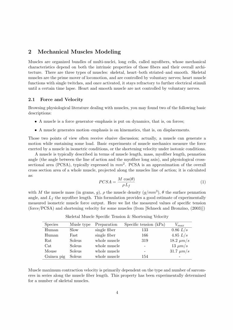
A muscle is typically described in terms of muscle length, mass, myofiber length, pennationangle (the angle between the line of action and the myofiber long axis), and physiological cross-sectional area (PCSA), typically expressed in mm2. PCSA is an approximation of the overallcross section area of a whole muscle, projected along the muscles line of action; it is calculatedas:

PCSA =M cos(θ)ρLf

(1)

with M the muscle mass (in grams, g), ρ the muscle density (g/mm3), θ the surface pennationangle, and Lf the myofiber length. This formulation provides a good estimate of experimentallymeasured isometric muscle force output. Here we list the measured values of specific tension(force/PCSA) and shortening velocity for some muscles (from [Schneck and Bronzino, (2003)])

Skeletal Muscle Specific Tension & Shortening Velocity

Species Musle type Preparation Specific tension (kPa) Vmax

Human Slow single fiber 133 0.86 L/sHuman Fast single fiber 166 4.85 L/sRat Soleus whole muscle 319 18.2 µm/sCat Soleus whole muscle - 13 µm/sMouse Soleus whole muscle - 31.7 µm/sGuinea pig Soleus whole muscle 154 -

Muscle maximum contraction velocity is primarily dependent on the type and number of sarcom-eres in series along the muscle fiber length. This property has been experimentally determinedfor a number of skeletal muscles.

4

2.2 Muscle as a Black Box

We present a list of wishful features for mechanical muscles modeling

• Less is more: a model should be as simple as possible.

• A muscle must control both position and force independently of each other; this requestrules out any standard elastic or viscoelastic response.

• Models with low dimension, as 0D (system of springs & dashpots) or 1D models (systemof bars), should be upgradable to a fully 3D models as smoothly as possible.

• Any kind of muscular workout requires energy; an adequate model should provide someinsight into energetics, and should predict energy consumption even in correspondence ofnull mechanical working.

L

f f

Figure 1: Muscle as a black box, exercising at length L while sustaining a load f .

Let us envision an exercising muscle as a black box, and let us describe the state of the muscleusing just two parameter: its visible length L(τ) and the load f(τ), a force, it sustains at agiven time τ . Many strain measures can be used to represent the length L(τ) in terms the slacklength Ls; among them, we have:

λ(τ) =L(τ)Ls

, ε(τ) =L(τ)− Ls

Ls= λ(τ)− 1 . (2)

We define

P(L) = f · L mechanical power done by external load f on muscle velocity L;

L =∫T f(τ) · L(τ) dτ mechanical work done during a time interval T ;

(3)a superposed dot denoting differentiation with respect to time.

2.3 Gym session

Isometric. From L = 0, it followsP(L) = 0. (4)

Isotonic. From f = 0, it follows

L = f ·∫

TL(τ) dτ = f ·∆L (5)

with ∆L = L(τ1)− L(τo), being T = (τo, τ1).

5

3 Hill’s equation for tetanized muscle

Hill’s equation, a celebrated equation in muscle mechanics, has been proposed by Hill in 1938[Hill, (1938)] after experiments on tetanized skeletal muscle from frog sartorius based on accuratecalorimetric measurements taken during a sudden change of muscular exercise, from isometricto isotonic conditions.

At first, a muscle bundle, clamped at one end, is electrically stimulated and mantained atfixed length Lo (isometric conditions) by the appropriate reaction force; eventually, a maximumforce Fo is reached. At this tetanized state, the reaction force is suddenly decreased to a constantvalue F ≤ Fo (isotonic conditions): it follows that the muscle contracts. The experimentis repeated with different initial length Lo and/or isotonic loads F , and the resulting meanshortening velocity V and time course of heat production h(τ) is registered.

Fo Fo

F F

Ls

Lo

L s

Figure 2: Schematic of Hill’s experiment: a muscle is tetanized at constant length Lo (top);then, it is left free to shorten a distance s under a constant load F < Fo until a given length L isreached (middle). During the shortening from Lo to L a measurable amount of heat is released.The green bar represents the slack length (bottom).

heat

tetanus

tens

ion

timeτs τt

isometric

isometric exercise

heat

isometric

constant shortening

F2F1

τs τt τ1 τ2 time

heat

isometric

constant loads2

s1

τs τt τ1 τ2 time

Figure 3: Stimulus starts at time τs and tetanus is reached at τt; heat rate in (τs, τt) is higherwith respect the rate after tetanus (left). Shortening starts at τt and stops at τi (i=1,2). Heatrate is proportional to the load (F2 > F1), but eventually the same amount of heat is released(middle). Shortening different distances (s2 > s1) under same load yields same heat rate; totalamount of heat released is proportional to distance (right).

6

Key findings by Hill (see Fig. 6,7 in [Hill, (1938)]) are represented in Fig.3, and listed in thefollowing:

• Isometric exercises show two distinct energetic regimes: heat is released at high rate im-mediately after activation, between stimulus and tetanus; after tetanus is reached, the rateat which heat is released becomes much smaller, see Fig. 3, left. It is worth noting thatisometric exercises are characterized by a same heat rate: after shortening, when muscleis back again in isometric regime, heat is released at the same rate as during the isometricbenchmark.

h = A Activation thermal-power, almost constant in (τs, τt);

h = B Tension-time thermal-power, with B < A (isometric exercise).(6)

• Isotonic exercises show a further different regime, characterized by large heat rates. Fig.3, (center, right), shows:

h > B heat rate during shortening is larger that isometric heat rate. (7)

• Shortening same distance under different loads shows that the amount of heat released doesnot depend on the load, while both heat rate and shortening velocity are proportional tothe load, see Fig. 3, center:

Vi = s/(τi − τt) ∝ Fi shortening velocity is proportional to load;

h ∝ V ∝ F shortening heat rate is proportional to load and thus to velocity.

(8)

• Shortening different distances under same load shows that heat rate during shorteningdoes not vary, while the amount of heat released is proportional to shortened distances.

h(τi) ∝ si heat released is proportional to distance shortened. (9)

We define the rate of extra energy liberation E during shortening as the sum of the shorten-ing thermal-power a V , and the mechanical power W expended by the isotonic load F on theshortening velocity V : W = F V . Experimental findings show that E is a linear function of thedifference between the load at tetanus Fo and the load sustained during isotonic shortening F

E = W + a V = b(Fo − F ) . (10)

Relation (10) yields the Hill’s equation in its original forms

(F + a)V = b (Fo − F ) or (V + b) (F + a) = b (Fo + a) ; (11)

it is worth noting that a is a force-like parameter, related to heat production during contrac-tion, while b is a velocity-like parameter. Let us note that, to an unloaded (F = 0) isotonic

7

condition, there corresponds a maximal shortening speed Vo = b Fo/a; thus, the parameter b canbe expressed in terms of the two measurable quantities Vo, Fo. Using this representation for b,equation (11) can be rewritten highlighting non dimensional ratios as follows:

(a+ F )V =Vo a

Fo(Fo − F ) ⇒ (1 +

F

a)V

Vo= 1− F

Fo. (12)

We then define the non dimensional quantities v = V/Vo, f = F/Fo, α = a/Fo and write anondimensional version of (12)

(1 +f

α) v = 1− f . (13)

The change of variables ξ = f + α, η = v + α yields the following hyperbolic function

ξ η = α (1 + α) . (14)

Hill’s equation contains three parameters, namely Fo, b, and a, or, alternatively, Fo, Vo andα; these parameters are function of the initial muscle length Lo, and of other experimentalconditions such as temperature and composition of physiological bath.

3.1 Isometric force-length relationship

A noteworthy dependence becomes apparent during the isometric exercise: a non-monotonerelationship between the isometric length Lo and the maximal force Fo. Let us denote with Ls

the slack length; a tetanized muscle cannot generate any appreciable force when Lo ≤ 0.6Ls;then, maximal force increases with Lo, until a plateau is reached for Lo ∼ Ls; then, maximalforce decreases again, and becomes negligible for Lo ≥ 1.8Ls. Thus, it happens that, in orderto develop the maximum force, a muscle must exercise around its slack length. The isometricforce-length curve was first presented in [Gordon et al., (1966)], and is showed in Fig.4.

Contrary to Fo, the other two parameters, Vo and α, do not show any appreciable dependenceon length Lo.

104

Biomechanics: Principles and Applications

As a result, tendons are more compliant at low loads and less compliant at high loads. The highlynonlinear low-load region has been referred to as the “toe” region and occurs up to approximately 3%strain and 5 MPa [Butler et al., 1979; Zajac, 1989]. Typically tendons have linear properties from about3% strain until ultimate strain which is approximately 10% (Table 5.7). The tangent modulus in thislinear region is approximately 1.5 GPa. Ultimate tensile stress reported for tendons is approximately 100MPa (Table 5.7). Tendons operate physiologically at stresses of approximately 5 to 10 MPa (Table 5.7).Thus, tendons operate with a safety factor of 10 to 20 MPa.

FIGURE 5.1

Sarcomere length-tension curve elucidated for isolated frog skeletal muscle fibers by Gordon, Huxley,and Julian [1966]. This demonstrates the length dependence of skeletal muscle on isometric strength.

FIGURE 5.2

Force-velocity relationship for isolated skeletal muscle for shortening and lengthening. These data areplots of Eqs. 5.1 and 5.2 normalized for the maximum contraction velocity of the muscle.

1492_ch05_Frame Page 104 Wednesday, July 17, 2002 10:59 PM

Figure 4: Sarcomere tension-length relation for isolated frog skeletal muscle.

8

4 Hill’s three-element model

Hill’s model represents a muscle as composed of two elastic elements acting in parallel; oneelement, dubbed passive, is a simple elastic spring; the other one, called active, is a springwhose ground length, that is, whose zero elastic-energy length, can be shortened; moreover, it isusually assumed that this active spring could sustain a force only under positive straining. Theforce exerted by the system is thus the sum of two contributions, which are related to the strainssuffered by the passive and the active springs. The model retains its name, three-element model,from the fact that originally the active component was conceived as composed of a spring anda contractile element in series, thus totaling three components.

LLp

εp

La

εa

f

f

LLp

εp

La

εa

δ

f

f

Figure 5: Hill’s model.

The model is zero-dimensional, and the state of the system is described, at any instant τ , bytwo variables:

L(τ) visible length of the two parallel elements,

La(τ) ground length of the active component;(15)

omitting the time dependence in the notation, we define the strains as:

∆Lp = L− Lp , passive strain; ∆La = L− La , active strain, (16)

where Lp is the ground length of the passive spring. The overall force f is the sum of a passiveforce fp and an active one fa; assuming linear elastic spring, we may write

f = fp + fa = kp ∆Lp + ka ∆LaH(∆La) , (17)

with kp and ka the stiffness of the passive and active springs, respectively, and H(·) the Heavisidefunction. We note that L = Lp = La yields ∆Lp = ∆La = 0 and thus f = 0; it follows that Lp

may be considered as the slack state for the system. We can define the actual ground length La

in terms of the shortening δ with respect to the slack length Lp:

La = Lp − δ , ∆La = L− Lp = ∆Lp + δ . (18)

9

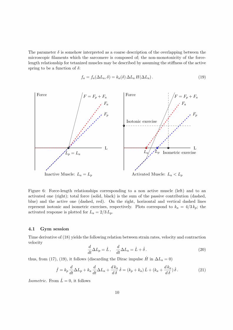
The parameter δ is somehow interpreted as a coarse description of the overlapping between themicroscopic filaments which the sarcomere is composed of; the non-monotonicity of the force-length relationship for tetanized muscles may be described by assuming the stiffness of the activespring to be a function of δ:

fa = fa(∆La, δ) = ka(δ) ∆LaH(∆La) . (19)

Inactive Muscle: La = Lp

Force

L

F = Fp + Fa

Fa

Fp

Lp = La

Isotonic exercise

Isometric exercise

Activated Muscle: La < Lp

Force

L

F = Fp + Fa

Fa

Fp

LpLa

Figure 6: Force-length relationships corresponding to a non active muscle (left) and to anactivated one (right); total force (solid, black) is the sum of the passive contribution (dashed,blue) and the active one (dashed, red). On the right, horizontal and vertical dashed linesrepresent isotonic and isometric exercises, respectively. Plots correspond to ka = 4/3 kp; theactivated response is plotted for La = 2/3Lp.

4.1 Gym session

Time derivative of (18) yields the following relation between strain rates, velocity and contractionvelocity

d

dt∆Lp = L ,

d

dt∆La = L+ δ . (20)

thus, from (17), (19), it follows (discarding the Dirac impulse H in ∆La = 0)

f = kpd

dt∆Lp + ka

d

dt∆La +

d ka

d δδ = (kp + ka) L+ (ka +

d ka

d δ) δ . (21)

Isometric. From L = 0, it follows

10

f = (ka +d ka

d δ) δ , (22)

that is, the time rate of force is proportional to contraction rate.Isotonic. From f = 0, it follows

L

δ= −

ka +d ka

d δkp + ka

, (23)

that is, visible velocity L and contraction velocity δ are related each other. For d ka/d δ = 0, itfollows that the two velocities must have different sign.

11

5 Active tension

Hill’s model dominated the field of mechanical muscle modeling since its proposal in 1938.Despite many improvements have been added, and full fledged 3D settings have been proposed,one key assumption still survive: the additive splitting of the force in a passive component andan active one.

Here, as prototypical example of enhanced muscle model developed in the cultural heritageof Hill’s model, we present that proposed in [Hunter et al., (1998)]; the model is aimed at inter-preting some experimental tests, and focuses on the relationships between the tension developedin a cardiac muscle and its physiological state, summarized by a coarse description of crossbridgekinetics. In particular, it focuses on the following mechanical experiments:

• tension-length relation in resting and activated muscles;

• time course of tension development under isometric conditions;

• tension recovery under length step tests (1% sudden shortening yields 100% tension drop);

• isotonic shortening at constant velocity (Hill experiments as benchmark);

• frequency response.

A key assumption is that the overall tension T sustained by a muscle be the sum of a passivecomponent Tp, described by an appropriate elastic energy (pole-zero law) based on biaxial testresults, plus an active component Ta, assumed to depend on the strain and the level of activation

T = Tp(strain) + Ta(strain, activation) . (24)

Most of the effort is done on the characterization of a response function for Ta(strain, activation),based on physiological phenomena and capable of describing the aforementioned mechanicalexperiments.

5.1 Physiology

Muscle physiology is described through the following phenomena: diffusion of free calcium ionsthrough the cell (intracellular ions, Cai); binding and release of calcium ions to Troponin C(bound ions, Cab); thin filaments kinetics (percentage of available actin sites, z).

free ions Cai ⇒ bound ions Cab ⇒ actin sites available z ⇒ active tension Ta . (25)

Ca2+ kinetics. Intracellular Calcium ions (Cai) is released from the junctional sarcoplasmaticreticulum (jSR) as a consequence of a twitch; it diffuses into the cell, and bounds to Troponin C(TnC) which in turn regulates myofilaments force development. The kinetics of Cai is assumedto be almost independent from the state of the muscle, and described once and for all by thefollowing relation

Cai = Cao + (Cam − Cao)τ

τcexp (1− τ/τc) . (26)

12

Figure 7: Schematic of tension-length relation for passive and active response of muscle. Thenon linear passive response Tp is added to a linear function whose intercept with vertical axisdepends on the activation level. From [Hunter et al., (1998)].

Relation (30) describes a fast increase of Cai from the resting level Cao to a maximum valueCam, attained at τ = τc, followed by a slower decay to the resting value.

TnC-Ca2+ binding kinetics. Binding of Cai to TnC is very fast and limited by diffusion throughthe cell; its release, in turns, depends on the state of the muscle. As example, isometric orisotonic twitches terminate differently, and the load sustained by a muscle may alter the releaserate. It follows that the amount of bound Calcium ions Cab should be sensible at least to theintracellular concentration Cai and to the load T sustained; moreover, binding and release shouldhave different time rates

Thin filaments kinetics. Binding of Cai to TnC triggers myosin–actin interactions; its macro-scopic effect is what is called ‘force generation’. The level of activation of the muscle should besensible to the percentage of actin sites available for cross-bridge binding

Moreover, a fading memory effect is included to capture some key features observed in exper-iments that involve vary fast responses, as in length step or frequency test. These effects aresomehow related to crossbridge kinetics.

5.2 State variables

The model is essentially 1D, and considers a bar of length ls, meant to represent the musclein its slack state, that is, unloaded and non activated. The muscle state is described by four

13

variablesl visible length;Cab concentration of bound Ca2+;z proportion of actin sites that are available for crossbridging.

(27)

Defined the strain λ = l/ls, and denoted with ψ(λ) the elastic energy density, we may write

T = Tp + Ta = ∂ψ(λ) + Ta(λ, z) . (28)

5.3 Evolution equations for physiological varibles

The physiological variables Cab and z satisfy two coupled evolution equations. Kinetics of boundions is described by

Cab = ρoCai (Cabm − Cab)− ρ1 (1− T

γ To)Cab . (29)

where ρo, ρ1 are binding and release rate constants, respectively, Cabm is the maximum value ofCab attained for T = γ To Kinetics of actin sites available is described by

z = αo

[(Cab

C50

)n

(1− z)− z]. (30)

where αo describes tropomyosin ‘mobility’, C50 is the value of bound ions yielding a 50% avail-ability, and n = n(λ) governs the steepness of the relation z 7→ z. For the active tension Ta. itis assumed a linear dependence on both the strain λ and the actin sites z

Ta = Tref (1 + βo (λ− 1) ) z . (31)

where Tref is the reference tension at λ = 1, and β a non dimensional parameter reflecting thestiffening effects of activated myofilaments.

14

6 Mechanics in a Page!

Kinematics.The motion of a body manifolds in the ambient space is described by state variables. Rigid

motions have a peculiar role; thus, a definition of strain is needed to discriminate those motionsfrom general ones. Definition of velocity and test velocity follows straightforward from the choiceof state variables.

u state variables ⇒ u velocity, u test velocity . (32)

Working.A force is primarily a continuous linear real-valued functional on the space of test velocities,

whose value is the working expended by that force. The assumption of any specific functionalexpresses a strong intention about the outcome of the mechanical model under development.

< force, test velocity >=< f, u >= P(u) power expended by f on u . (33)

Balance law.All balance laws are systematically provided by the principle of null working: the total

working expended on any test velocity should be zero, i.e., the total force should be the nullfunctional.

P(u) = 0 , ∀u . (34)

Constitutive issues.Working is additively split into inner, outer, and inertia working:

P(u) = P in(u) + Pout(u)− P ine(u) . (35)

Two fundamental principles are enforced to deliver strict selection rules on the constitutiveprescription for the inner actions. Such a priori restrictions do not apply to the outer actions,which are regarded as adjustable controls on the process.

Constitutive principle #1: material indifference to change in observer.Inner working must be indifferent to change in observer:

P in(u) = P in(u∗) , ∀ u , u∗ related by a change in observer . (36)

Constitutive principle #2: dissipation principle.Along any realizable process, the time rates of kinetic energy (k) plus free energy (ψ) must

be less or equal the outer power expended along the same process.

k(u) + ψ(u) ≤ Pout(u) = P ine(u)− P in(u) , ∀ realizable process τ 7→ u(τ) . (37)

By definition, k(u) = P ine; thus dissipation principle can be re-formulated as

ψ(u) ≤ −P in(u) , ∀ realizable process τ 7→ u(τ) . (38)

or, introducing a dissipation functional D(u) = −(ψ(u) + P in(u)), by asserting that the powerdissipated should be non-negative, for all body-parts, at all times, along all processes.

15

7 Active Contraction: 1D setting

We model a muscle as a single elastic bar, whose rest length can change. It is worth noting thatthe main difference with respect to the Hill’s three element model will rely on dynamics, as weshall consider the rest length of the bar as an additional kinematical descriptor; in this sense,we may say that this model is endowed with a double-layer kinematics. The omission of thepassive bar is just a minor issue.

7.1 State variables

We consider a bar of length ls, meant to represent the muscle in its slack state, that is, unloadedand non activated, and assuming the bar to be uniformly stretched, we describe its state usingtwo kinematical variables, that we call extended motion: p = (l, lo), with

l visible length;lo ground length.

(39)

We can introduce three stretch measures: two compares the ground and visible lengths withrespect to the slack one; the last one compares the actual and the ground length (see Fig. 8):

λ =l

ls(visible) stretch;

λo =lols

active stretch;

ϕ =l

lo=

l

ls

lslo

= λλ−1o total stretch.

(40)

slack

ground

visible

l

lol − lo

ls l − ls

ls − lo

f f

slack

ground

visible

λ

λo

ϕ = λλ−1o

f f

Figure 8: Schematic of the muscle model. The load f sustained during activation depends onthe difference between the visible and the ground length. Cartoon at right shows the role of thethree stretch measures.

16

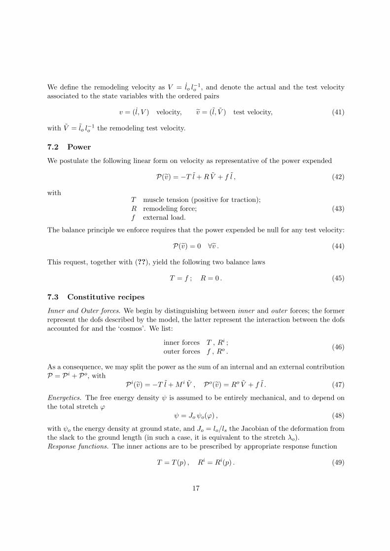
We define the remodeling velocity as V = lo l−1o , and denote the actual and the test velocity

associated to the state variables with the ordered pairs

v = (l, V ) velocity, v = (l, V ) test velocity, (41)

with V = lo l−1o the remodeling test velocity.

7.2 Power

We postulate the following linear form on velocity as representative of the power expended

P(v) = −T l +R V + f l , (42)

withT muscle tension (positive for traction);R remodeling force;f external load.

(43)

The balance principle we enforce requires that the power expended be null for any test velocity:

P(v) = 0 ∀v . (44)

This request, together with (??), yield the following two balance laws

T = f ; R = 0 . (45)

7.3 Constitutive recipes

Inner and Outer forces. We begin by distinguishing between inner and outer forces; the formerrepresent the dofs described by the model, the latter represent the interaction between the dofsaccounted for and the ‘cosmos’. We list:

inner forces T , Ri ;outer forces f , Ro .

(46)

As a consequence, we may split the power as the sum of an internal and an external contributionP = P i + Po, with

P i(v) = −T l +M i V , Po(v) = Ro V + f l . (47)

Energetics. The free energy density ψ is assumed to be entirely mechanical, and to depend onthe total stretch ϕ

ψ = Jo ψo(ϕ) , (48)

with ψo the energy density at ground state, and Jo = lo/ls the Jacobian of the deformation fromthe slack to the ground length (in such a case, it is equivalent to the stretch λo).Response functions. The inner actions are to be prescribed by appropriate response function

T = T (p) , Ri = Ri(p) . (49)

17

Dissipation Principle. Any constitutive prescription for T (p), Ri(p) must satisfy the followingdissipation principle: along any realizable motion τ 7→ p(τ), the time rate of the free energymust be less or equal than the power expended by the external actions, which in turn, is theopposite to the internal power

ψ ≤ Po(v) = −P i(v) , ∀v (50)

The dissipation principle stands as an explicit regulation governing the selection of appropriateconstitutive prescriptions.Reduced dissipation. We write here some useful relations, consequences of (40) and (48):

l = (ϕ lo)˙ = ϕ lo + ϕ lo = (ϕ+ ϕV ) lo , Jo =lols

= Jo V . (51)

Thus, from (50), with (48) and (49), it follows a reduced dissipation inequality

[ Jo ψo(ϕ)− ϕT (p) lo +Ri(p) ] V + [ Jo ψ′o(ϕ)− T (p) lo ] ϕ ≤ 0 . (52)

We now define

So(p) = J−1o T (p) lo reference tension;

Sd(p) = ψ′o(ϕ)− So(p) dissipative tension;

E(p) = ψo(ϕ)− ϕSo(p) Eshelby-like tension;

Rd(p) = JoE(p) +Ri(p) dissipative remodeling force.

(53)

and rewrite (52) as followsRd(p) V + Sd(p) ϕ ≤ 0 . (54)

Let us note that the Eshelby-like tension constitutes a key coupling between the remodeling innerforce Ri and the tension So. A further assumption that tension is purely energetic, Sd(p) = 0,and dissipative remodeling is viscous-like, yields constitutive prescriptions for So(p), Ri(p), andE(p) that identically satisfy (54)

Sd(p) = 0

Rd(p) = − VM

, M > 0⇒

So(p) = ψ′o(ϕ)

Ri(p) = −(JoE(p) +V

M)

E(p) = ψo(ϕ)− ϕψ′o(ϕ)

(55)

We can now write balance in equations in terms of the motion

Jo ψ′o(ϕ) l−1

o = f balance of force;

V = M (Ro − JoE) balance of remodeling force.(56)

We conclude this presentation by considering a K-L like energy

ψo =12k (ϕ2 − 1)2 . (57)

18

It follows:So(p) = 2 k ϕ (φ2 − 1) reference tension;

T (p) = Jo k ϕ l−1o = . . . tension;

E(p) = . . . Eshelby-like tension.(58)

7.4 Gym session

We deal with the following evolution equations

1lsk ϕ = f balance of force;

V = M (Ro +lolsk ϕ2) balance of remodeling force.

(59)

Let us note that both visible and ground lengths are involved in tension development

T = T (l, lo) , (60)

thus, we can control both load and position independently from each other.

Isometric. From l = 0, it follows ϕ lo + ϕ lo=0. A remodeling force such that Ro = −lo/ls k ϕ2

yields V = 0 and thus, lo = 0

f = (ka +d ka

d δ) δ (61)

that is, the time rate of force is proportional to contraction rate.Isotonic. From f = 0, it follows ϕ = l/lo − l lo/l

2o = 0; thus, isotonic exercise can be done

providedl

l=lolo, (62)

that is, visible velocity l and contraction velocity lo are related each other.

19

8 Active Contraction: 3D setting

We shall briefly present non linear elasticity with growing large distortions, as presented in[DiCarlo and Quiligotti,(2002)]. The evolution of distortion is used to describe muscle contrac-tion as in [Nardinocchi and Teresi, (2007)], [DiCarlo et al., (2009)].

9 Kinematics

9.1 Motion

Let B be the body manifold (identified with its reference shape), T the time line, E the 3DEuclidean ambient space, with VE the associated vector space, Lin = VE ⊗VE = Sym⊕Skw thespace of double tensors on VE (linear maps of VE into itself). An extended motion is describedby the pair motion and distortion (p,Fo); the motion is a position-valued fieldd field

p : B ×T → E (63)(X, t) 7→ x = p(X, t) = X + u(X, t) (64)

associating to any material point X ∈ B its position in space x = p(X, t) ∈ E ; the vector-valuedfield u = x −X represents the displacement of the material point X. The set Bt = p(B, t) isthe actual configuration of B at time t. The distortion is a tensor-valued field

Fo : B ×T → Lin (65)(X, t) 7→ Fo(X, t) (66)

endowed with a noteworthy constitutive assumption: the image of body elements under Fo arevolume elements at ground state, that is at zero elastic energy. Let us remark the distortions arenot required to be compatible, not even locally, that is, a ground configuration may not exists.

Given a motion (p,Fo), the associated exended velocity and extended test velocity are givenby

(p, Fo F−1o ) , (p, Fo F−1

o ) . (67)

Key geometrical functions are performed by the gradient of the motion F, its adjugate F∗, andits Jacobian determinant J :

F :=∇p = I +∇u ,

F∗ := J F−> ; (68)

J := det(F) .

Let a hierarchy of infinitesimally small one-, two-, and three-dimensional parallelepipedal cells,built out of the vectors a, b, c ∈ VE , be attached to a place X ∈ B :

i) a line element , gauged by the vector a ;

ii) a facet (a, b) , gauged by its Gibbs representative a×b ; and

20

iii) a volume element (a, b, c) , gauged by its (oriented) volume a×b · c .

Then, their images under the action of p, obviously attached to x = p(X, t) , are gauged respec-tively by:

i) F(X, t) a ;

ii) F∗(X, t)(a×b) = (F(X, t) a)×(F(X, t) b) ;

iii) J(X, t)(a×b · c) = (F(X, t) a)×(F(X, t) b)·(F(X, t) c) .

Let us note that from (ii), it follows a rule relating the oriented normal m to a facet and theoriented normal n to the image of that facet

n =F∗m|F∗m|

. (69)

Finally, introducing a standard notation for line, surface and volume elements, we may write

dx = F dX , da = |F∗m| dA , dv = J dV. (70)

The same geometrical functions are performed by the distortion Fo, its adjugate F∗o and itsJacobian determinant Jo, with the important caveat that, in general, it does not exists anydisplacement uo such that I +∇uo = Fo.

9.2 Anisotropic distortions

Let us note that it is possible to define transversely-anisotropic distortion field Fo: denoted withe a unit vector field, we have

Fo = λ‖ e⊗ e + λ⊥ (I− e⊗ e) . (71)

Here λ‖ measures the contraction along the fibers, and λ⊥ a possible deformation orthogonal tothe fibers, whose choice represents an important constitutive assumption; it is worth associatingthe parameter λ⊥ to the variation of volume Jo = det Fo induced by the distortion, and write

λ⊥ =

√Jo

λ‖; (72)

Jo = 1 yields a volume preserving contraction, while Jo = λ‖ yields a uni-axial one; in such acase, we have

Fo = I + (λ‖ − 1) e⊗ e . (73)

21

f = Fo eFoe

F

Fe = Fe f

Fe = FF−1o

Figure 9: Deformations F and distortions Fo suffered by a material fiber e.

9.3 Elastic Deformation

We define the elastic deformation Fe of the body elements as the difference between the distor-tions Fo and the visible deformations F in the sense of multiplicative composition:

Fe = FF−1o ; (74)

it is worth noting that Fo and Fe are not, in general, gradients of any fields. We define thefollowing three different metric tensors to be used as strain measures (left Cauchy-Green strains):

C = F>F , Ce = F>e Fe = F−>o CF−1o , Co = FT

o F . (75)

Let us note that C and Co measure the strain suffered by a reference fibre e once embedded inthe actual state or distorted, respectively; alternatively, Ce measures the strain λe suffered bya distorted fiber f embedded in the actual state, see Fig. 9:

e 7→ f = Fo e , Fe = FF−1o ⇒ λ2

e = Fe f · Fe f = Ce · f ⊗ f = Fe · Fe = C · e⊗ e . (76)

10 Elastic Energy

Let us introduce three different stress measures

S reference stress, aka, first P-K ;

So ground stress ;

T “the stress”, aka, actual or Cauchy stress .

(77)

The reference stress S is related to the other ones by a pull-back as follows

S = TF∗ = So F∗o . (78)

We assume that the hyperelastic response of the body is described by a strain energy densityper unit ground volume ψo whose value at each body point X ∈ B depends only on the present

22

ψo , Soe =∂ψo

∂FeFo

S = TF∗ = So F∗o

ψ = Jo ψo , Se =∂ψ

∂F

F

T = J−1 SFT

Fe = FF−1o

Figure 10: Stress measures and energy densities.

value of the elastic deformation Fe at that point; moreover, we assume the elastic deformationto be isochoric:

ψo : Fe 7→ ψo(Fe) , & Je = det(Fe) = 1 . (79)

Given ψo, the strain energy density per unit reference volume is defined by ψ = Jo ψo, withJo = det(Fo); the energetic part of the stress is thus defined by

Soe :=∂ψo

∂Fe, ground measure ; Se :=

∂ψ

∂F, reference measure . (80)

We have, see Fig. 10:

Se = Soe F∗o , pull back of the energetic stress ;

S = Se + Sv , with Sv = −pF∗ , reference stress ;

T = S (F∗)−1 = Se (F∗)−1 − p I , actual stress .

(81)

Here p denotes the indeterminate pressure, reaction to the isochoric constraint. Let us note thatenergy is usually represented in terms of the strain measure Ce or Ee = 1/2(Ce − I); from therepresentation formula for the time rate of Ce, Ee

Ce = FTe Fe + FT

e Fe = 2 sym(FTe Fe) , Ee = Ce/2 . (82)

we have the following useful relation between energy derivatives:

ψo =∂ψo

∂Ce· Ce = 2 Fe

∂ψo

∂Ce· Fe =

∂ψo

∂Fe· Fe ⇒ Soe =

∂ψo

∂Fe= 2 Fe

∂ψo

∂Ce= Fe

∂ψo

∂Ee. (83)

The derivative of the energy with respect to Ee is usually dubbed as the second P-K stress:

∂ψo

∂Ee= F−1

e Soe . (84)

23

Finally, let us note that from ψ = Jo ψo, it follows

ψ =∂ψ

∂F︸︷︷︸Se

·F = Jo∂ψo

∂Fe· Fe = Jo

∂ψo

∂FeF−>o · Fe =

∂ψo

∂Fe︸︷︷︸Soe

F∗o · Fe . (85)

Remark: Here, we have assumed distortions as given once and for all; by assuming distortionalprocesses t 7→ Fo(t) you need to consider their time derivative, and this yields noteworthyconsequences on balance equations.

24

11 Attach-detach-contract model (release 2.8)

We model a muscle as a telescoping unit, composed by two bars, overlapping each other to someextent, that we dub attach-detach-contract model, as presented in [DiCarlo, (2008)]; moreover,we assume one of the two bars to be active, that is, endowed with a variable ground length.

s

la

lp

l

f

f

Figure 11: adc’s model.

11.1 State variables

We assume the bars to be uniformly stretched, and we describe the system using four statevariables, that we call extended motion p = (lp, la, s, lo), with

lp passive-bar (p-bar) length;la active-bar (a-bar) length;s overlapping between p- and a-bars;lo ground length of the a-bar.

(86)

The overall length of the system, that is, its visible length, is given by

l = la + lm − s . (87)

The stretches in the bars are defined as the ratios between their actual and relaxed length

λa =lalo, λp =

lpl∗p, (88)

with l∗p the ground length of the p-bar, given once and for all. We denote the (actual) velocityand the test velocity associated to the state variables with the ordered quadruplets

v = (la, lm, s, lo) velocity;

v = (la, lm, s, lo) test velocity;(89)

given (87), we may represent the visible velocity l in terms of v as follows: l = la + lm − s.

25

11.2 Power

Power is a linear form on velocity; prompted by the ‘serial’ disposition of the elements, wepostulate the following representation formula for the power expended

P(v) = −Ta la − Tp lp + C s+R lo + f l , (90)

withTa , Tm tension (positive for traction);C coupling force (between a- and m-elements);R remodeling force:f external load.

(91)

The balance principle we enforce requires that the power expended be null for any test velocity:

P(v) = 0 ∀v . (92)

This request, together with (87), yield the following four balance laws

Ta = Tp = C = f ; R = 0 . (93)

11.3 Constitutive recipes

Inner and Outer forces. We distinguish between inner and outer forces:

inner forces Ta , Tp , C , Ri ;

outer forces f , Ro .(94)

As a consequence, we may split the power as the sum of an internal and an external contributionP = P i + Po, with

P i(v) = −Ta la − Tp lp + C s+Ri lo , Po(v) = Ro lo + f l . (95)

Energetics. The free energy density, assumed to be entirely mechanical, is defined as the sum ofthe elastic energies of the two bar

ψ = ψa(λa) + ψp(λp) (96)

Response functions. The inner actions are prescribed by appropriate response function

Ta = Ta(p) , Tp = Tp(p)) , C = C(p) , Ri = Ri(p) , (97)

Dissipation Principle. We enforce that, along any realizable motion τ 7→ p(τ), the time rate ofthe free energy be less or equal than the power expended by the external actions, which in turn,is the opposite to the internal power

ψ ≤ Po(v) = −P i(v) , ∀v (98)

26

Inserting relations (95), (96) and (97) in (98), it follows a reduced dissipation inequality

[ψ′a1lo− Ta(p) ] la + [ψ′p

1l∗p− Tp(p) ] lp + C(p) s+ [Ri(p)− ψ′a

lal2o

] lo ≤ 0 . (99)

A further assumption that no dissipation is related to Ta, Tp, yields

Ta(p) = ψ′a(λa)1lo, Tp(p) = ψ′p(λp)

1l∗p, C(p) s+Rd(p) lo ≤ 0 , (100)

with Rd(p) a dissipative term, endowed with an Eshelbian coupling between elasticity, ψ′a, andremodeling force, Ri, given by

Rd(p) = Ri(p)− ψ′a(λa)lal2o

= Ri(p)− Ta(p)λa . (101)

Thus, it remains to prescribe a constitutive recipe for the coupling force C(p) and the innerremodeling action Ri(p), such that (103)3 hold. A simple recipe fitting the reduced dissipationinequality is as follows

C(p) = − 1M

s , Rd(p) = −D lo, , with M > 0 , D > 0 . (102)

In such a case, reduced dissipation inequality rewrites as

− s2

M−D lo ≤ 0 . (103)

11.4 Evolution equations.

s = −M f

D lo = λa Ta(λa) +Ro

0 = −Ta(λa) + f

(104)

27

References

[Hill, (1938)] Hill, A.V., 1938. The heat of shortening and the dynamic constants of muscle.Proc R Soc London B Biol Sci 126: 136-195.

[Huxley, 1957] Huxley A.F., 1957. Muscle structure and theories of contraction. Prog BiophysBiophys Chem 7: 255-318.

[Gordon et al., (1966)] Gordon, A.M., Huxley, A.F., Julian, F.J., 1966. The variation in iso-metric tension tension with sarcomere length in vertebrate muscle fibers. J. Physiol. 185,170–192.

[Hunter et al., (1998)] Hunter P.J., McCulloch A.D., ter Keurs H.E.D.J., 1998. Modelling theMechanical properties of cardiac muscle. Prog. Biophys. Molec. Bio. 69, 289–331.

[DiCarlo, (2008)] DiCarlo A., 2008. Elementary mechanics of muscular exercise. Mini-Workshop:The mathematics of growth and remodelling of soft biological tissues, MathematischesForschungsinstitut Oberwolfach Report 39/2008, 2232–2235

[DiCarlo and Quiligotti,(2002)] DiCarlo A., Quiligotti S., 2002. Growth & Balance. MechanicsRes. Comm. 29:449–456.

[Nardinocchi and Teresi, (2007)] Nardinocchi P., Teresi L., 2007. On the Active Response ofSoft Living Tissues. J. Elasticity, 88:27–39.

[DiCarlo et al., (2009)] A. DiCarlo, P. Nardinocchi, T. Svaton, L. Teresi, 2009. Passive andactive deformation process in cardiac tissue. In Proceedings of the Int. Conf. on Computa-tional Methods for Coupled Problems in Science and Engineering (COUPLED PROBLEMS2009), Eds. B. Schreer, E. Onate and M.Papadrakakis, CIMNE, Barcelona.

[Schneck and Bronzino, (2003)] Schneck D.J., Bronzino J.D., 2003. Biomechanics. Principlesand Applications. CRC Press.

28