clean and wipe - astronomy and astrophysics · a. lannes et al.: clean and wipe 185 the rst point...

ASTRONOMY & ASTROPHYSICS MAY II 1997, PAGE 183

SUPPLEMENT SERIES

Astron. Astrophys. Suppl. Ser. 123, 183-198 (1997)

CLEAN and WIPEA. Lannes, E. Anterrieu, and P. Marechal

Laboratoire d’Astrophysique (and CERFACS),Observatoire Midi-Pyrenees, 14, Avenue Edouard Belin, F-31400 Toulouse, France

Received March 14; accepted July 22, 1996

Abstract. Clean is a matching pursuit process whichhas two weak points: in situations of astrophysical inter-est, the “clean map” is not stable in the correspondingobject representation space, and the “atoms” of this rep-resentation (translated versions of the “clean beam”) arenot well suited for reconstructing the boundaries of thestructuring entities of the object at the related resolutionlevel. As a result, Clean must be interrupted before thebest possible fit is reached. How does Wipe wipe Clean

clean? First, by introducing a global regularization prin-ciple based on the concept of resolution; and second, byconducting the matching pursuit process at the level ofthe high-resolution basis functions of the object space.

Key words: methods: data analysis; numerical —techniques: image processing; interferometric

1. Introduction

WIPE is a Fourier synthesis method recently de-veloped in radio imaging and optical interferometry(Lannes et al. 1994, 1996). The name of Wipe is associatedwith that of CLEAN, a deconvolution method intensivelyused in astronomy (Hogbom 1974; Schwarz 1978). (WIPE

can also be used as a deconvolution technique.) As a mat-ter of fact, WIPE was devised, quite independently, on thegrounds of well known properties in harmonic analysis andband-limited interpolation (Lannes et al. 1987a). Therealso exists a probabilistic interpretation of this method(Marechal & Lannes 1997). Nevertheless, to some extent,Wipe can equally well be regarded as an updated versionof CLEAN. This paper is aimed precisely at clarifying therelationship between these two methods.

In Sect. 2, we first show that Clean lies in the familyof “matching pursuit” techniques (Mallat & Zhang 1993).In other words, the principle of the “iterative harmonicanalysis” of CLEAN, as it is exhibited in Schwarz (1978),can be regarded as a special case of a more general ap-proach. We then present the reconstruction methods that

Send offprint requests to: A. Lannes

can be implemented for solving the related optimizationproblems, first, without any control of the propagation oferrors (Sect. 3), and afterwards, with a complete controlof the stability parameters (Sect. 4). The first weak pointof Clean can thus be exhibited: in situations of astro-physical interest (for example, when observing extendedcomplex objects with dilute apertures), the matching pro-cess of Clean is ill-conditioned. As shown in Sect. 5,the regularization principle of WIPE, which can be ap-plied to Clean as it is, remedies this lack of robustness.Unfortunately, Clean has another weak point: the ba-sis functions used in the matching pursuit process, the‘clean beams,’ are not well suited for reconstructing theboundaries of the structuring entities of the images at theselected resolution level. As a result, Clean must be inter-rupted before the best possible fit is reached. As indicatedin Sect. 5, the basic version of Wipe overcomes this diffi-culty in a simple and efficient manner. The multiresolutionextension of WIPE, underlying the main aspects of this pa-per, reinforces the arguments justifying this methodolog-ical choice.

The guiding idea of our analysis is based on the the-oretical framework presented in Sect. 1.1. (The readerwho is not familiar with the related basic notions is in-vited to consult Appendices 1 to 4 of Lannes et al. 1987a).As Clean was first used as a Fourier synthesis tech-nique, it was natural to compare the principles of Clean

and WIPE in this context. Such a comparative study canonly be started from a common statement of the problem.The corresponding formulation, which makes the theoret-ical framework more attractive, is presented in Sect. 1.2.We then also specify the general conditions of the numer-ical simulations in support of our analysis.

1.1. Theoretical framework

In many inverse problems, the “reconstructed object” isdescribed in an “object representation space” E generatedby m vectors gk selected among a family Eo of M vectorsg1, g2, . . . , gM . The latter may be regarded as the “atoms”of the object representation under consideration. The lin-ear space generated by all the vectors of Eo , Eo, is a sub-space of some Euclidean space: the “object space” Ho.

184 A. Lannes et al.: CLEAN and WIPE

The “data vector” ψd lies in another Euclidean space: the“data space” Kd. (When the data are complex quantities,it is always possible to work in the real linear space un-derlying the complex linear space directly involved in theanalysis.) To a first approximation, ψd is related to theobject (or image) to be reconstructed via a linear oper-ator A from Ho into Kd. The basic problem is to choosethe vectors gk in Eo , and thereby to construct the objectrepresentation space E. The solutions are then obtainedby minimizing on E the quadratic functional:

q : Ho → R, q(φ)4= ‖ ψd − Aφ ‖

2d . (1)

Clearly ‖ · ‖d= (· | ·)1/2d is the norm on Kd; the scalar

products on Ko and Kd, as well as the norms, will be dis-tinguished by the subscripts o and d, respectively.

Let F be the “image” of E by A (the space of the Aφ’s,φ spanning E), AE be the operator from E onto F in-duced by A, and ψF be the projection of ψd onto F(see Fig. 1). The vectors φ minimizing q on E, the solu-tions of the problem, are such that AEφ = ψF . They areidentical up to a vector lying in the kernel of AE . Note thatkerAE = E ∩kerA. (By definition, the kernel of A, kerA,also referred to as the null space of A, is the set of vec-tors φ such that Aφ = 0). The condition dimE ≤ dimKd

is a necessary condition for kerAE to be reduced to {0}.As ψd − ψF is orthogonal to F , the solutions φ of the

problem are characterized by the property:

∀ϕ ∈ E, (Aϕ | ψd −Aφ)d = 0 (φ ∈ E).

On denoting by A∗ the adjoint of A, this property canalso be written in the form

∀ϕ ∈ E, (ϕ | r)o = 0 r4= A∗(ψd − Aφ) (φ ∈ E),

where r is regarded as a residue. The solutions φ aretherefore characterized by the fact that the correspond-ing residue is orthogonal to E, i.e.,

∀gk ∈ E , (gk | r)o = 0. (2)

This condition is of course equivalent to PE r = 0,where PE is the projection (operator) of Ho onto E. Thesolutions of the problem are therefore the solutions of theequation on E:

PEA∗AE φ = PEA

∗ψd . (3)

For any ϕ ∈ E and any ψ ∈ Kd, we have

(Aϕ | ψ)d = (ϕ | A∗ψ)o = (ϕ | PEA∗ψ)o ,

hence A∗E = PEA∗. This explicitly shows that Eq. (3) is

the “normal equation”:

A∗EAE φ = A∗Eψd . (4)

When the problem is well posed, AE is a one-to-onemap (kerAE = {0}); the solution is then unique: there

exists only one vector φ ∈ E such that AEφ = ψF . Thisvector, φE, is said to be the least-squares solution of theequation AEφ “=” ψd.

In this case, let δψF be a variation of ψF in F ,and δφE be the corresponding variation of φE (see Fig. 1).As shown in Appendix 1, the robustness of the reconstruc-tion process is then governed by the inequality

‖ δφE ‖o‖ φE ‖o

≤ κE‖ δψF ‖d‖ ψF ‖d

(5)

where κE is the condition number of AE :

κE4=

√µ′√µ

; (6)

µ and µ′ respectively denote the greatest lower bound andthe least upper bound of ‖ AEφ ‖2d for the φ’s with normunity in E:

µ4= inf‖φ‖o=1

‖ AEφ ‖2d µ′

4= sup‖φ‖o=1

‖ AEφ ‖2d . (7)

The closer to 1 is the condition number, the easier andthe more robust is the reconstruction process. As

‖ AEφ ‖2d= (φ | A∗EAE φ)o ,

µ and µ′ are the smallest and largest eigenvalues ofA∗EAE ,respectively.

Fig. 1. Uniqueness of the solution and robustness of the re-construction process. Operator A is an operator from the ob-ject space Ho into the data space Kd. The object represen-tation space E is a particular subspace of Ho (see text). Theimage of E by A, the range of AE , is denoted by F . In thisEuclidean representation, ψF is the projection of the datavector ψd onto F . The inverse problem must be stated sothat AE is a one-to-one map from E onto F , the conditionnumber κE having a reasonable value (see Eq. (5))

In the analysis of the different methods that can bedevised and implemented for solving the problem, threemain aspects must be examined:

1) the precise definition of ψd, A and E;2) the selected minimization technique;3) the robustness of the reconstruction process.

A. Lannes et al.: CLEAN and WIPE 185

The first point is essential for the interpretation of the re-sults. It is related to the statement of the problem and,if need be, to its “regularization;” ψd is not necessarilythe vector of the experimental data. In such a case, thedefinition of A must of course take into account the cor-responding manipulations. As regards E, which may alsobe involved in the regularization of the problem, it is im-portant to note that this space may be constructed, in aglobal manner or step by step, interactively or automati-cally. As suggested by the statement of point 2, many dif-ferent techniques can be used for minimizing q on E; someof these are certainly more efficient than others, but in thiscase, the choice is not crucial. The last point concerns thestudy of the propagation of errors. The part played by in-equality (5) in the development of the corresponding erroranalysis shows that a good reconstruction procedure mustalso provide, in particular, the condition number κE .

1.2. Formulation of the problems of Fourier synthesis inastronomy

In the problems of Fourier synthesis encountered in as-tronomy, the “object function” of interest, φo, is a real-valued function of an angular position variable ξ =(ξ1, ξ2). The “object model variable” φ lies in some ob-ject space Ho whose vectors, the functions φ, are definedat a very high level of resolution. In this sense, one maysay that Ho emulates the Hilbert space of square inte-grable real-valued functions L2

R(R2). More precisely, Ho

is characterized by two key parameters: the extension∆ξ of its field, and its resolution scale δξ; δξ is there-fore much smaller than the resolution limit that can bereasonably expected at the end of the reconstruction pro-cess: δξ

4= ∆ξ/N , where N is some power of 2. (The larger

is N , the more oversampled is the object field.) To definethe object space more explicitly, we introduce the finitegrid (see Fig. 2):

G 4= L× L, L 4={p ∈ Z : −

N

2≤ p ≤

N

2− 1

}.

Let p be an integer vector lying in Z2: p = ( p1, p2).Clearly, the functions

ep(ξ)4= e0(ξ − p δξ) (8)

where

e0(ξ)4= sinc

( ξ1δξ

)sinc

( ξ2δξ

)(9)

form an orthogonal set with

‖ ep ‖2o= (δξ)2 (∀p ∈ Z2). (10)

In our comparative analysis of Clean and WIPE, Ho

is the Euclidean space generated by the basis vectors ep,

p spanning G (see Fig. 2). The functions φ lying in thisspace can therefore be expanded in the form:

φ =∑p∈G

xpep (xp ∈ R). (11)

In the general context of this paper, the functions ep,which play the role of interpolation or scaling functions,can be regarded as the “elementary particles” of theobject representation. Evidently, other orthogonal setsof scaling functions can be used (cf. Sect. 4.3 of Lanneset al. 1994). Let us finally note that Ho is a subspaceof L2R(R2); its inner product can be explicitly expressed

in the form (cf. Eqs. (8)-(11)):

(φ1 | φ2)o = (δξ)2∑p∈G

x1,p x2,p .

Thus,

‖ φ ‖2o= (δξ)2∑p∈G

x2p.

Fig. 2. Object grid G δξ for N = 8

The Fourier transform of φ is defined by the relation-ship

φ(u)4=

∫φ(ξ) exp(−2iπu · ξ) dξ,

where u is a two-dimensional angular spatial frequency:u = (u1, u2). According to Eqs. (11), (8) and (9), we there-fore have:

φ =∑p∈G

xpep

where

ep(u) = e0(u) exp(−2iπp ·

u

∆u

)


with ∆u4= 1/δξ and

e0(u) =1

(∆u)2rect

( u1

∆u

)rect

( u2

∆u

).

The “experimental data” ψe(u) are blurred valuesof φo(u) on a finite list of frequencies in the Fourierdomain: Le

4= {ue(1),ue(2), . . . ,ue(Ne)}. As φo is a

real-valued function, it is natural to define ψe(−u) as thecomplex conjugate of ψe(u). The ‘experimental frequencylist’ Le is defined consequently: if u ∈ Le, then −u ∈ Le

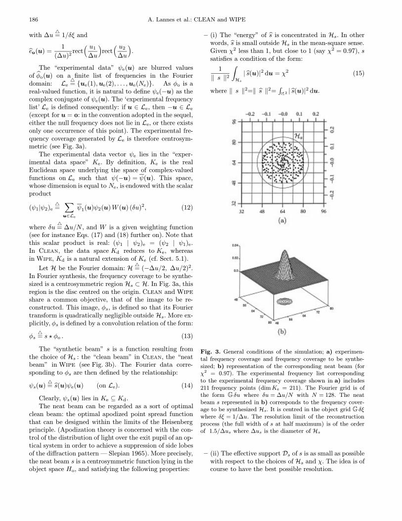
(except for u = : in the convention adopted in the sequel,either the null frequency does not lie in Le, or there existsonly one occurrence of this point). The experimental fre-quency coverage generated by Le is therefore centrosym-metric (see Fig. 3a).

The experimental data vector ψe lies in the “exper-imental data space” Ke. By definition, Ke is the realEuclidean space underlying the space of complex-valuedfunctions on Le such that ψ(−u) = ψ(u). This space,whose dimension is equal to Ne, is endowed with the scalarproduct

(ψ1|ψ2)e4=∑u∈Le

ψ1(u)ψ2(u)W (u) (δu)2, (12)

where δu4= ∆u/N , and W is a given weighting function

(see for instance Eqs. (17) and (18) further on). Note thatthis scalar product is real: (ψ1 | ψ2)e = (ψ2 | ψ1)e.In CLEAN, the data space Kd reduces to Ke, whereasin WIPE, Kd is a natural extension of Ke (cf. Sect. 5.1).

Let H be the Fourier domain: H4= (−∆u/2, ∆u/2)2.

In Fourier synthesis, the frequency coverage to be synthe-sized is a centrosymmetric region Hs ⊂ H. In Fig. 3a, thisregion is the disc centred on the origin. Clean and Wipe

share a common objective, that of the image to be re-constructed. This image, φs, is defined so that its Fouriertransform is quadratically negligible outside Hs. More ex-plicitly, φs is defined by a convolution relation of the form:

φs4= s ? φo . (13)

The “synthetic beam” s is a function resulting fromthe choice of Hs : the “clean beam” in CLEAN, the “neatbeam” in Wipe (see Fig. 3b). The Fourier data corre-sponding to φs are then defined by the relationship:

ψs(u)4= s(u)ψe(u) (on Le). (14)

Clearly, ψs(u) lies in Ke ⊆ Kd.The neat beam can be regarded as a sort of optimal

clean beam: the optimal apodized point spread functionthat can be designed within the limits of the Heisenbergprinciple. (Apodization theory is concerned with the con-trol of the distribution of light over the exit pupil of an op-tical system in order to achieve a suppression of side lobesof the diffraction pattern — Slepian 1965). More precisely,the neat beam s is a centrosymmetric function lying in theobject space Ho, and satisfying the following properties:

– (i) The “energy” of s is concentrated in Hs. In otherwords, s is small outside Hs in the mean-square sense.Given χ2 less than 1, but close to 1 (say χ2 = 0.97), ssatisfies a condition of the form:

1

‖ s ‖2

∫Hs

| s(u)|2 du = χ2 (15)

where ‖ s ‖2=‖ s ‖2=∫R2 | s(u)|2 du.

Fig. 3. General conditions of the simulation; a) experimen-tal frequency coverage and frequency coverage to be synthe-sized; b) representation of the corresponding neat beam (forχ2 = 0.97). The experimental frequency list correspondingto the experimental frequency coverage shown in a) includes211 frequency points (dimKe = 211). The Fourier grid is ofthe form G δu where δu = ∆u/N with N = 128. The neatbeam s represented in b) corresponds to the frequency cover-age to be synthesized Hs. It is centred in the object grid G δξwhere δξ = 1/∆u. The resolution limit of the reconstructionprocess (the full width of s at half maximum) is of the orderof 1.5/∆us where ∆us is the diameter of Hs

– (ii) The effective support Ds of s is as small as possiblewith respect to the choices of Hs and χ. The idea is ofcourse to have the best possible resolution.


– (iii) The normalization condition s(0) = 1, so that:∫R2

φs(ξ) dξ =

∫R2

φo(ξ) dξ. (16)

In the terminology adopted in this paper, an atom suchas s is a finite linear combination of elementary parti-cles ep. The integers p involved in this linear combinationlie in a subset Ds of G (see Figs. 2 and 3b). As explicitlyshown in Sect. 2 of Lannes et al. (1996), the computationof the corresponding coefficients does not raise any par-ticular difficulty.

In a first approach to Fourier synthesis, Eq. (13) sug-gests that the basis functions of the object representationspace E should be translated versions of s: a finite numberof atoms centred on the nodes of grid G. This very naturalidea, which is exploited as it is, in the matching pursuitprinciple of Clean (cf. Sect. 2.2), may be completely re-laxed in WIPE. More precisely, the matching pursuit pro-cess may be performed at the level of the elementary par-ticles. The resolution limit of the reconstruction processis then kept under control thanks to an appropriate regu-larization principle (cf. Sect. 5.1).

The simulations presented in this paper correspond tothe general conditions defined in Fig. 3. The “object func-tion” φo was defined as a set of “δ functions” centred onthe nodes of grid G δξ with N = 128. The image to be re-constructed (φs = s ? φo) then lies in Ho. Figure 4 givesan idea of the complexity of this image.

Fig. 4. Image to be reconstructed, φs, at the resolution leveldefined in Fig. 3. Note that the portion of the field representedhere is twice as large as that defined in Fig. 3b

The Fourier data were blurred by adding a Gaussiannoise. More precisely, for all the u ∈ Le (see Fig. 3a),

the standard deviation of [ψe(u) − φo(u)] was set equal

to 5% of the total flux of the object: σe(u) = φo()/20.The weighting function W introduced in Eq. (12) was ex-plicitly defined by the formula

W (u)4=

w(u)∑u′∈Le

sinc2(u1 − u′1

δu

)sinc2

(u2 − u′2δu

)w(u′)

(17)

where

w(u)4= 1/σ2

s(u), σs(u)4= s(u)σe(u). (18)

2. Reconstruction via matching pursuit methods

Among the various iterative methods that can be imple-mented for finding an approximation to the image (or theobject) to be reconstructed, there exists a very slow al-gorithm which is based on a matching pursuit strategy.As will be clarified in this section, this algorithm is noth-ing but an aborted version of a particular algorithm mini-mizing q on Eo (see the introduction of Sect. 1.1). The cor-responding iterative process must never be used in prac-tice for solving the problem. Its slow convergence mayhowever be of interest for initializing the choice of theobject representation space E. It is therefore importantto analyse its principle (Sect. 2.1), and in particular, toshow that Clean is an algorithm of this type (Sect. 2.2).

2.1. Reconstruction principle

Let hj4= Agj be the virtual data vector corresponding to

the object atom gj (cf. Sect. 1.1), and Qj be the projec-tion (operator) of Kd onto the space generated by hj :

Qjψ = η2j (hj | ψ)d hj (ψ ∈ Kd) (19)

where

ηj4= ‖ hj ‖

−1d = ( gj | A

∗Agj)−1/2o . (20)

The guiding idea is to determine the projection of ψd

onto Fd4= AEo via the elementary projections Qj.

Let us consider the iteration in Fd:

ψ0 = 0, ψn+1 = ψn + ωQk(ψd − ψn), (ω > 0); (21)

ω is a relaxation parameter to be defined. At each itera-tion, k ≡ kn is chosen so that

‖ Qk(ψd − ψn) ‖d= max1≤j≤M

‖ Qj(ψd − ψn) ‖d . (22)

If Qk(ψd − ψn) = 0, then ψn = ψFd (the projectionof ψd onto Fd) and the problem is solved.

Let us set yn4= ψd − ψn and zn

4= ψFd − ψn. As

Qkyn = Qkzn, we have from Eq. (21):

yn+1 = yn − ωQkyn zn+1 = zn − ωQkzn.

It follows that

‖ yn+1 ‖2d =‖ yn ‖

2d −2ω(yn | Qkyn)d + ω2 ‖ Qkyn ‖

2d

=‖ yn ‖2d −2ω ‖ Qkyn ‖

2d +ω2 ‖ Qkyn ‖

2d ,

hence

‖ yn+1 ‖2d=‖ yn ‖

2d −ω(2 − ω) ‖ Qkyn ‖

2d . (23)


Likewise, ‖ zn+1 ‖2d=‖ zn ‖2d −ω(2 − ω) ‖ Qkzn ‖2d.Provided that ω lies in the open interval (0, 2), ω(2− ω)is strictly positive. Then, ‖ zn+1 ‖d≤‖ zn ‖d. The se-quence {βn}∞n=0, where βn

4= ‖ zn ‖2d, therefore con-

verges towards some nonnegative number β. As shown inAppendix 2, β proves to be equal to 0. As a result, zn → 0as n→∞. The iterates (21) then converge towards ψFd .

The maximal value of ω(2 − ω) is attained for ω = 1.To increase the convergence speed of the projectionoperation, ω may be set equal to this optimal value.The corresponding algorithm, ψn+1 = ψn +Qk(ψd − ψn),is nothing but a traditional matching pursuit process(see Mallat & Zhang 1993).

As yn = ψd − ψn, we have from Eq. (19),

Qkyn = η2k (Agk | ψd − ψn)dAgk ,

hence

Qkyn = η2k ( gk | rn)oAgk (24)

where rn4= A∗(ψd − ψn). The relaxed matching pursuit

iteration (21) can therefore be written in the form

ψ0 = 0, ψn+1 = ψn + ωη2k( gk | rn)oAgk .

Clearly, this sequence is the image by A of the objectsequence (in Eo):

φ0 = 0, φn+1 = φn + ωη2kρn,k gk , (25)

where

ρn,k4= ( gk | rn)o rn = A∗ψd − A

∗Aφn . (26)

According to its definition, the residue rn is obtainedvia the iteration:

r0 = A∗ψd , rn+1 = rn − ωη2kρn,kA

∗Agk . (27)

As, from Eqs. (24) and (26), Qkyn = η2kρn,kAgk , we

have (cf. Eq. (20)):

‖ Qkyn ‖2d= η4

kρ2n,k( gk | A

∗Agk)o = η2kρ

2n,k .

On setting (cf. Eq. (1))

qn4= q(φn) =‖ ψd − Aφn ‖

2d =‖ ψd − ψn ‖

2d=‖ yn ‖

2d ,

it follows from Eq. (23) that qn is obtained through theiteration:

q0 =‖ ψd ‖2d , qn+1 = qn − ω(2− ω)η2

kρ2n,k . (28)

Provided that ω lies in the open interval (0, 2), theiterates qn converge towards the minimal value of q on Eo.Sequence (25) then converges towards a solution φ of theproblem; φ is the unique solution φEo , if and only if AEo isa one-to-one map.

2.2. Presentation of CLEAN as a matching pursuitalgorithm

In our formulation of CLEAN, which essentially fol-lows that of Hogbom (1974), the object space is theEuclidean space Ho introduced in Sect. 1.2. The vectors gjare then translated versions of the clean beam CB ≡ s(see Fig. 3b). More precisely, the elements of Eo are theclean beams CBp centred on the nodes of the “cleanbox” Gc δξ:

CBp ≡ sp , sp(ξ)4= s(ξ − p δξ) (p ∈ Gc ⊂ G).

The data space Kd coincides with the experimentaldata space Ke, and A with the experimental Fourier sam-pling operator: (Aeφ)(u)

4= φ(u) on Le. As the image to

be reconstructed is defined as the convolution of the orig-inal object by the clean beam (Eq. (13)), the data vec-tor ψd must be defined as the experimental data vec-tor ψe damped by the Fourier transform of the cleanbeam: ψd = ψs (cf. Eq. (14)). We then have q ≡ qe with(cf. Eqs. (1), (12) and (17)):

qe(φ)4= ‖ ψs −Aeφ ‖

2e

=∑u∈Le

|ψs(u)− φ(u)|2W (u) (δu)2. (29)

As explicitly shown in Appendix 3, the “dirty map”is the map of the scalar components of A∗eψe in thebasis of the elementary particles ep. In this context,A∗eψs may be referred to as the “dusty map”. For clar-ity, we set DMe ≡ A∗eψe and DMs ≡ A∗eψs. Likewise, theaction of A∗eAe corresponds to a “discrete convolution” bythe “dirty beam” DB: A∗eAeφ = DB ? φ (the precise def-inition of this operation is given in Appendix 3). Thus,from Eq. (20), the parameters η p ≡ ηj are all equal to:

η = (CB | DB ? CB)−1/2o . (30)

The relaxed matching pursuit iteration (25) can thenbe written in the form

φ0 = 0, φn+1 = φn + ωη2ρn,p CBp , (31)

where (from Eq. (26))

ρn,p = (CBp | rn)o rn = DMs −DB ? φn . (32)

Clearly, ρn (the map of the ρn,p) is nothing but the“discrete intercorrelation” of rn with CB.

The residue rn and the quadratic errors qn are respec-tively obtained via the iterations (27) and (28):

r0 = DMs , rn+1 = rn − ωη2ρn,p(DB ? CBp) (33)

and

qe,0 =‖ ψs ‖2e=

∑u∈Le

|ψs(u)|2W (u) (δu)2,

qe,n+1 = qe,n − ω(2 − ω)η2ρ2n,p . (34)


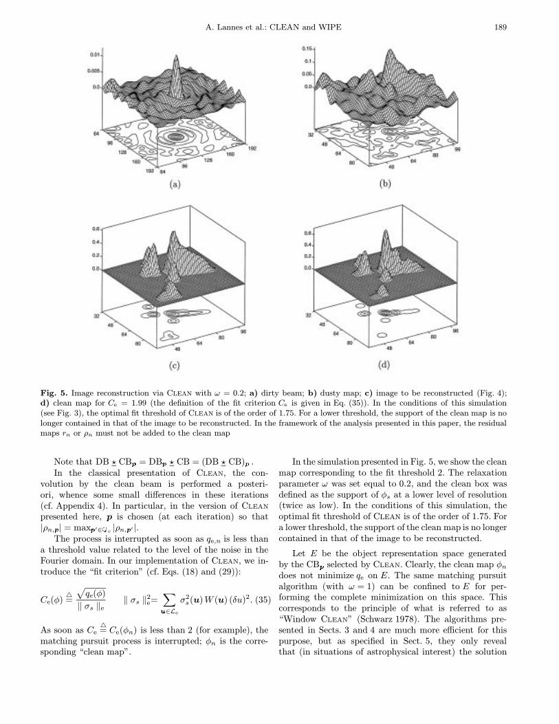
Fig. 5. Image reconstruction via Clean with ω = 0.2; a) dirty beam; b) dusty map; c) image to be reconstructed (Fig. 4);d) clean map for Ce = 1.99 (the definition of the fit criterion Ce is given in Eq. (35)). In the conditions of this simulation(see Fig. 3), the optimal fit threshold of Clean is of the order of 1.75. For a lower threshold, the support of the clean map is nolonger contained in that of the image to be reconstructed. In the framework of the analysis presented in this paper, the residualmaps rn or ρn must not be added to the clean map

Note that DB ? CBp = DBp ? CB = (DB ? CB)p .In the classical presentation of CLEAN, the con-

volution by the clean beam is performed a posteri-ori, whence some small differences in these iterations(cf. Appendix 4). In particular, in the version of CLEAN

presented here, p is chosen (at each iteration) so that|ρn,p| = maxp′∈Gc |ρn,p′ |.

The process is interrupted as soon as qe,n is less thana threshold value related to the level of the noise in theFourier domain. In our implementation of CLEAN, we in-troduce the “fit criterion” (cf. Eqs. (18) and (29)):

Ce(φ)4=

√qe(φ)

‖ σs ‖e‖ σs ‖

2e=

∑u∈Le

σ2s(u)W (u) (δu)2. (35)

As soon as Ce4= Ce(φn) is less than 2 (for example), the

matching pursuit process is interrupted; φn is the corre-sponding “clean map”.

In the simulation presented in Fig. 5, we show the cleanmap corresponding to the fit threshold 2. The relaxationparameter ω was set equal to 0.2, and the clean box wasdefined as the support of φs at a lower level of resolution(twice as low). In the conditions of this simulation, theoptimal fit threshold of Clean is of the order of 1.75. Fora lower threshold, the support of the clean map is no longercontained in that of the image to be reconstructed.

Let E be the object representation space generatedby the CBp selected by CLEAN. Clearly, the clean map φndoes not minimize qe on E. The same matching pursuitalgorithm (with ω = 1) can be confined to E for per-forming the complete minimization on this space. Thiscorresponds to the principle of what is referred to as“Window CLEAN” (Schwarz 1978). The algorithms pre-sented in Sects. 3 and 4 are much more efficient for thispurpose, but as specified in Sect. 5, they only revealthat (in situations of astrophysical interest) the solution


thus obtained is without any interest: the problem is ill-conditioned.

3. Optimization without control of robustness

Let E be any subset of Eo, say that generated byan aborted matching pursuit process; E has m elements.Let us now consider the problem of minimizing q(φ) onthe space E generated by the gk, k spanning

J 4= {k : gk ∈ E}.

By definition, E is the range of the operator:

S : Rm → Ho , Sα4=∑k∈J

αkgk . (36)

In the case where Rm is equipped with its standard scalarproduct, the adjoint of S is explicitly defined by the rela-tionship:

(S∗φ)k = (gk | φ)o (for all k ∈ J).

Indeed, for any φ ∈ Ho, we have from Eq. (36):

(Sα | φ)o =∑k∈J

αk (gk | φ)o ≡∑k∈J

αk (S∗φ)k .

In what follows, S is not necessarily a one-to-one mapfrom Rm onto E: the vectors gk lying in E are not neces-sarily linearly independent.

Let α now be a vector minimizing on Rm the quan-tity ‖ ψd −ASα ‖2d . Then, the vector φ = Sα mini-mizes q on E. From Eq. (2), the vectors α in question aresuch that

∀k ∈ J,(gk | A

∗(ψd − ASα))

o= 0. (37)

These vectors are therefore the solutions of the normalequation

S∗A∗(ψd −ASα) = 0 (α ∈ Rm) (38)

(the least-squares solutions of the equation ASα “=” ψd).In most cases encountered in image reconstruction,

the conjugate-gradients method is the best suited tech-nique for solving Eq. (38). The version of this method pre-sented below provides φ = Sα.

ALGORITHM 1:

Step 0: Set ε = 10−6 (for example) and n = 0;choose a natural starting point φ0 in E;compute r0 = A∗ψd − A∗Aφ0,

q0 =‖ ψd −Aφ0 ‖2d;compute ρ0,k = ( gk | r0)o (for all k ∈ J);set δ0,k = ρ0,k (for all k ∈ J).

Step 1: Computedn =

∑k∈Jδn,kgk,

zn = A∗Adn,

ζn,k = ( gk | zn)o (for all k ∈ J),

ωn =∑k∈J|ρn,k|

2/∑k∈Jδn,kζn,k,

qn+1 = qn − (2rn − ωnzn | ωndn)o,

φn+1 = φn + ωndn,

rn+1 = rn − ωnzn,

ρn+1,k = ρn,k − ωnζn,k (for all k ∈ J);

if maxk∈J{|ρn+1,k|/ ‖ gk ‖o} < ε ‖ rn+1 ‖o,termination.

Computeγn =

∑k∈J|ρn+1,k|2/

∑k∈J|ρn,k|

2,

δn+1,k = ρn+1,k + γnδn,k (for all k ∈ J);

increment n and loop to step 1.

Throughout this algorithm, rn is the residue of the equa-tion A∗ψd − A∗Aφ = 0 for φ = φn. Likewise, qn is thevalue of q(φ) at the same iterate:

rn = A∗ψd −A∗Aφn , qn =‖ ψd − Aφn ‖

2d .

The iteration in qn results from the identity:

q(φ+ δφ) = q(φ)− 2(ψd − Aφ | Aδφ)o+ ‖ Aδφ ‖2d= q(φ)− 2(A∗ψd −A

∗Aφ | δφ)o

+(A∗Aδφ | δφ)o.

The sequence of vectors φn converges towards a solu-tion of the problem with all the remarkable properties ofthe conjugate-gradients method (see Lannes et al. 1987b).In practice, E is chosen so that AE is a one-to-one map.The uniqueness of the solution can easily be verified bymodifying the starting point of the algorithm. The stop-ping criterion is based on the fact that the final residuemust be practically orthogonal to all the gk’s (Eq. (37));the cosine of the angle between the vectors rn and gk isequal to ρn,k/(‖ gk ‖o ‖ rn ‖o). Here, as Rm is endowedwith its standard scalar product, this algorithm cannotprovide the condition number of AE . (The transpositionof what is presented in Sect. 4.2 would give the “general-ized condition number” of AS). We therefore recommendto use algorithm 1 only when κE is approximately known.

REMARK 3. Let us consider the special case where A is theidentity operator on Kd (which then coincides with Ho).The problem is then to find PEφd, the projection ofφd = ψd onto E. Note that κE is then equal to unity. Inthis case, algorithm 1 reduces to

ALGORITHM 2:

Step 0: Set ε = 10−6 (for example) and n = 0;set φ0 = 0 and r0 = φd;computeq0 =‖ φd ‖2o,


ρ0,k = ( gk | r0)o (for all k ∈ J);set δ0,k = ρ0,k (for all k ∈ J).

Step 1: Computezn =

∑k∈Jδn,kgk,

ζn,k = ( gk | zn)o (for all k ∈ J),

ωn =∑k∈J|ρn,k|

2/∑k∈Jδn,kζn,k,

qn+1 = qn − (2rn − ωnzn | ωnzn)o,

φn+1 = φn + ωnzn,


ρn+1,k = ρn,k − ωnζn,k (for all k ∈ J);

if maxk∈J{|ρn+1,k|/ ‖ gk ‖o} < ε ‖ rn+1 ‖o,termination.

Computeγn =

∑k∈J|ρn+1,k|2/

∑k∈J|ρn,k|

2,

δn+1,k = ρn+1,k + γnδn,k (for all k ∈ J) ;

increment n and loop to step 1.

This algorithm converges towards the projection of φd

onto E with all the properties of the conjugate-gradientsmethod.

In principle, the projection operation can also be per-formed by using the matching pursuit iteration (25). Inthis case, on setting ω equal to its optimal value, this it-eration reduces to

φ0 = 0, φn+1 = φn + η2kρn,kgk ,

where

ηk =‖ gk ‖−1o ρn,k = ( gk | rn)o rn = φd − φn .

The residues rn are then obtained via iteration (27):

r0 = φd , rn+1 = rn − η2kρn,kgk ;

and likewise for qn (cf. Eq. (28)):

q0 =‖ φd ‖2o , qn+1 = qn − η

2kρ

2n,k .

At each iteration, it is then natural to choose k sothat ηk|ρn,k| = maxj∈Jηj|ρn,j|. In the general case wherethe gk’s (k ∈ J) do not form an orthogonal set, theconjugate-gradients algorithm is of course preferable.

4. Optimization with control of robustness

For clarity, let us now assume that AE is a one-to-onemap. The method presented in Sect. 3 then yields a solu-tion α of Eq. (38), and thereby the solution of the prob-lem: φE = Sα. Unfortunately, as already mentioned, thismethod does not provide any information on the robust-ness of the reconstruction process. The most natural way

of obtaining this information is to find φE, directly, as thesolution of the normal Eq. (4):

Bφ = φd , (39)

where

B4= A∗EAE = PEA

∗AE φd4= A∗Eψd = PEA

∗ψd . (40)

In this section, we present the corresponding de-velopments. To conduct our analysis, the eigenvaluesof B are ordered so as to form a nondecreasing sequence(cf. Eq. (7)):

µ4= µ1 ≤ µ2 ≤ · · · ≤ µ

′ 4= µm . (41)

As AE is assumed to be a one-to-one map, µ is strictlypositive. In the general case where the gk generating E donot form an orthogonal set, the reader must keep in mindthe fact that the action of PE can be performed with theaid of algorithm 2.

4.1. Reconstruction algorithm

The problem is solved by using the conjugate-gradientsmethod (cf. Sect. 2.3 of Lannes et al. 1987b). Startingfrom any φ0 in E, the iterates φn converge to φE in atmost m iterations, φn getting closer to φE at each itera-tion. In this algorithm, dn is the “direction of research” initeration n+ 1, whereas ωn is the corresponding “param-eter of exact line search”; rn is the residue of the normalEq. (39) for φ = φn:

rn4= φd − Bφn.

As BφE = φd, we have rn = B(φE − φn), hence:

‖ φE − φn ‖o≤1

µ‖ rn ‖o .

Denoting by µe an estimate of µ, we therefore have:

‖ φE − φn ‖o‖ φn ‖o

<∼ εn, εn4=‖ rn ‖o

µe ‖ φn ‖o.

Let us introduce an acceptable error threshold εφ for‖ φE − φn ‖o / ‖ φn ‖o. Clearly, the iterative process canbe interrupted as soon as εn is less than εφ; εn thereforeplays the role of a convergence estimator. The estimateof µ is refined throughout the iterative process as indi-cated in Sect. 4.2. The corresponding algorithm can thenbe summarized as follows.

ALGORITHM 3:

Step 0: Set εφ = 10−4 (for example) and n = 0;choose a natural starting point φ0 in E;compute r0 = φd − Bφ0;set d0 = r0.

Step 1: Compute


zn = Bdn,

ωn =‖ rn ‖2o /(dn | zn)o,

φn+1 = φn + ωndn,


εn+1 =‖ rn+1 ‖o /(µe ‖ φn+1 ‖o);

if εn ≤ εφ, termination.

Computeγn =‖ rn+1 ‖2o / ‖ rn ‖

2o,

dn+1 = rn+1 + γndn.

Increment n and loop to step 1.

4.2. Effective object representation space

In the conjugate-gradients method, the n-dimensionalsubspace of E generated by the conjugate directionsd0 , . . . , dn−1,

En4= span{d`}

n−1`=0 ,

is referred to as the Krylov space of order n. According toa well known property (cf. properties 2 and 3.1 of Lanneset al. 1987b), φn minimizes q(φ) on En.

Provided that n is sufficiently large, the least-squaressolutions in E and En are very close to one another.At the end of the reconstruction process, En is thereforethe effective object representation space. The dimension ofthis space, as well as the robustness of the reconstructionprocess, depends upon the localization of the eigenvaluesof B, and more precisely, on the relative weight of the pro-jections of r0 onto the corresponding eigenspaces. We arethus led to consider the operator

Bn:En→ En , Bnφ4= PnA

∗Aφ,

where Pn is the projection (operator) onto En.The residues r0 , . . . , rn−1 form an orthogonal basis

for En (see Appendix 4 of Lannes et al. 1987b). As estab-lished in Appendix 2 of Lannes et al. (1996), the matrixof Bn expressed in this basis is tridiagonal (this matrixis of course symmetric). Its diagonal and upper-diagonalelements are respectively given by the relationships

bn;`,` =

1

ω`(` = 0)

1

ω`+γ`−1

ω`−1(1 ≤ ` ≤ n − 1)

and

bn;`−1, ` = −

√γ`−1

ω`−1(1 ≤ ` ≤ n− 1).

The eigenvalues of Bn can therefore be calculated veryeasily with the aid of the QR algorithm (cf. Sect. 11.3 of

Press et al. 1992). Let us order these eigenvalues as thoseof B (see Eq. (41)):

µn,1 ≤ µn,2 ≤ · · · ≤ µn,n .

By referring to the eigenvalue analysis based on thenotion of “minmax numbers” (cf. Appendix 5 of Lanneset al. 1987a), it is easy to show that

µ ≤ µn+1,1 ≤ µn,1 , µn,n ≤ µn+1,n+1 ≤ µ′.

Provided that the projections of φd onto theeigenspaces corresponding to µ and µ′ are different fromzero, a condition which is always numerically satisfied inpractice, µn,1 and µn,n respectively tend to µ and µ′ as ntends to m (see Fig. 3 of Lannes et al. 1996).

In our reconstruction processes, the eigenvalues of Bnare computed at each iteration. (The cost for this is neg-ligible compared to that of the action of B.) As soonas (µn,1 − µn+1,1)/µn,1 is less than say 10−3,

µe = µn,1 , µ′e = µn,n ,

are very good approximations to µ and µ′, respectively. Inmost cases, the termination test of the basic algorithm isthen satisfied (see Fig. 3 of Lannes et al. 1996).

5. How WIPE wipes CLEAN clean

We now have all the tools for analysing the weak pointsof Clean as well as the tricks of WIPE allowing the corre-sponding difficulties to be overcome.

In situations of astrophysical interest, Clean is imple-mented with a value of the relaxation parameter ω muchless than 1 (say 0.2). The basis vectors sp selected in thematching pursuit process then define an acceptable ob-ject representation space E. Unfortunately, the problemis often ill conditioned; AE is a one-to-one map, but itscondition number is very large. For example, in the sim-ulation presented in Fig. 5d, κE is equal to 45.08. As aresult, φE is a very perturbed version of the clean map.This is unsatisfactory. Indeed, in this situation, the cleanmap can only be regarded as an image for which thefit criterion Ce (introduced in Eq. (35)) is of the orderof the threshold value (say 2). In other words, the cleanmap must be accepted as it is, without any reference toa stable optimization process. The interpretation of theresults may then be doubtful. As indicated in Sect. 5.1,the regularization principle of WIPE remedies this lack ofrobustness, but the regularized version of Clean thus ob-tained is still different from WIPE. Indeed, Clean hasanother weak point: the boundaries of the structuring en-tities of the image may not be correctly represented inthe clean map. In such situations, the matching pursuitstrategy of Clean is not well suited for solving the prob-lem. For example, in the particular case of the Fourierdata of our simulation, the best possible fit corresponds


Fig. 6. Image reconstruction via the regularized version of Clean; a) traditional clean map for Ce = 1.99; b) improved cleanmap φE provided by the regularized version of Clean (Ce = 1.15). These images have to be compared with the image to bereconstructed (Fig. 5c). As shown in Fig. 7b, the matching pursuit process of Wipe can still refine image (b)

to a value of Ce of about 0.9 (see Fig. 7 further on). Evenwith a good support constraint (a reasonable “clean box”),CLEAN cannot reach this fit threshold with a satisfactoryrepresentation of the image support. In the same situa-tion, as shown in Sect. 5.2, WIPE reaches this thresholdwithout any difficulty.

5.1. How WIPE regularizes CLEAN

In the basic version of Clean presented in Sect. 2.2, thefunctions φ ∈ E are linear combinations of atoms sp.In the sense defined in Sect. 1.2, the “energy” of theFourier transform of each atom sp is concentrated in Hs(cf. Eq. (15)). The intrinsic instability of Clean is relatedto the fact that this property does not necessarily hold forany linear combination of such atoms. This difficulty arisesany time the distances between these atoms are muchsmaller than the corresponding resolution limit. This isprecisely the case when dealing with extended objects anda small relaxation parameter ω.

To overcome this difficulty, WIPE suggests that Clean

should define the reconstructed image as the function min-imizing on E the functional

q(φ)4= qe(φ) + qr(φ) (42)

where (see Eq. (29))

qe(φ)4=∑u∈Le

|ψs(u)− φ(u)|2W (u) (δu)2

and

qr(φ)4=∑u∈Lr

|φ(u)|2 (δu)2. (43)

The experimental criterion qe constrains φ (the model)to be consistent with the damped Fourier data, whilethe regularization criterion qr penalizes the high-frequencycomponents of φ. The elements of the regularization fre-quency list Lr are located outside Hs, at the nodes ofgrid Hr δu where

Hr4= {r ∈ Z2 : r δu ∈ H, r δu /∈ Hs}.

In the traditional version of CLEAN, q reducesto qe. The minimization of qe on E then reveals the ill-conditioned character of the problem.

The regularized version of Clean corresponding to cri-terion (42) can be formulated in the theoretical frameworkpresented in Sect. 1.1. To clarify this point, let us intro-duce the data vector:

ψd(u)4=

{ψs(u) on Le;0 on Lr.

This vector lies in a data space Kd endowed with thescalar product:

(ψ1 | ψ2)d4=

∑u∈Le

ψ1(u)ψ2(u)W (u) (δu)2

+∑u∈Lr

ψ1(u)ψ2(u) (δu)2.

The Fourier sampling operator A is then the operator:

A:Ho→ Kd , (Aφ)(u)4=

{φ(u) on Le;

φ(u) on Lr.

According to Eqs. (42), (29) and (43), q(φ) can then beeffectively written in the form ‖ ψd − Aφ ‖2d (see Eq. (1)).


The problem is then stated in terms of Fourier interpola-tion (Lannes et al. 1987a and 1994). This is why q is of theform qe+αqr with α = 1. In this context, it is important tonote that in the definition of qe (Eq. (29)), where ψs is de-fined in Eq. (14), the weighting function W (u) takes intoaccount the local redundancy of u up to δu (Eq. (17)).

The algorithms described in Sects. 3 and 4 can be usedfor minimizing q on E. The action of A∗A is that of aconvolutor. The corresponding point spread function, the“dusty beam”, has two components: the dirty beam andthe “regularization beam”. The latter is induced by theregularization list Lr. With regard to the dusty map, notethat A∗ψd ≡ A∗eψs (cf. Sect. 2.2).

In the simulation presented in Fig. 6, we compare theclean map of Fig. 5d (for which Ce = 1.99) with the imageprovided by this opt(Ce = 1.15). The condition number isnow reasonable: κE = 2.62. As shown in the next subsec-tion, the construction of the object representation space Ecan, however, be refined.

5.2. How WIPE relaxes the matching pursuit process ofCLEAN

In the regularized version of Clean described in Sect. 5.1,the calculation of the condition number κE requires theaction of the projection PE at each iteration of algo-rithm 3. This projection is performed at the cost of theconjugate-gradients iterations of algorithm 2. This firstremark suggests that E should be redefined as the lin-ear space generated by the elementary particles ep′ ofall the atoms sp selected in the matching pursuit pro-cess of CLEAN. The projection onto E is then trivial sincethese elementary particles form an orthogonal set. As theresolution limit of the reconstruction process is then con-trolled by the regularizer qr (cf. Eq. (43)), the choice ofsuch an object representation space proves to be very nat-ural. Moreover, the definition of E can then be refined bycontinuing (or even by conducting) the matching pursuitprocess at the level of the elementary particles. As speci-fied below, this is what is precisely done in WIPE.

Let D then be the subset of G corresponding to thechoice of E . (The elementary particles generating E arecentred on the nodes of D δξ.) We say that D is the “dis-crete field (or support)” associated with the definitionof E. Depending on the particular problems to be solved,this discrete field may be fixed from the outset (for exam-ple, in an interactive manner), or constructed step by stepin a matching pursuit strategy.

In this last case, which corresponds to the basic ver-sion of WIPE, let us denote by D(i) the discrete field ob-tained at the end of the i th step of the construction of theobject representation space. Let φ(i) then be the solutionof the problem in the corresponding object representationspace E(i). In the basis of the elementary particles ep (the

interpolation basis of Ho), the scalar components of theresidue r(i) are the quantities:

ρ(i)p

4= (ep | r

(i))o r(i) 4= A∗ψs −A∗Aφ(i) .

According to the definition of φ(i) , these coefficientsvanish on D(i) (see Eq. (2) with gk ≡ ep, p ∈ D(i)). Onethen has to decide whether the current field has to be ex-tended. The current values of Ce and κE play an essentialrole in this decision. When the reconstruction procedureis not interrupted at this stage, WIPE uses algorithm 3 forcomputing the solution of the problem in the object rep-resentation space relative to the union of D(i) with someset D′ ⊂ G:

D(i+1) = D(i) ∪ D′.

There exist many ways of selecting D′. All are based on

the examination of the distribution of the coefficients ρ(i)p

outside D(i). For example, one may try to define D′ as aconnected region containing the “pixel” pmax for which themaximum of these coefficients is attained. The simplestchoice is then to define D′ as the discrete field of the atom scentred on this pixel. With regard to the construction ofthe object representation space, the corresponding versionof Wipe is then very similar to that of Clean.

In the matching pursuit steps where the field of the re-constructed image must be refined, it is natural to choosethe nodes of D′ along the boundaries of the structuringentities of the image. Let Ns be the number of particles in-volved in the linear combination defining the neat beam s(the number of nodes in Ds). In the basic version of WIPE,the size of D′, expressed in number of nodes, is defined as afraction of Ns (say Ns/2), and the selected nodes are those

for which the coefficients ρ(i)p are the largest above some

given threshold (half of the maximal value, for example).The field of the image (or object) to be reconstructed canthus be obtained in a natural manner.

The construction of the object representation spaceis interrupted as soon as the fit criterion Ce(φ

(i)) is suf-ficiently small, for instance, less than or of the orderof 0.85. The current field is then refined by a morpholog-ical smoothing of its connected entities. In this classicaloperation of mathematical morphology, the discrete sup-port of the neat beam, Ds, is of course used as structuringelement. The boundaries of the effective field of the “neatmap” (the reconstructed image) are thus defined at theappropriate resolution. In particular, the connected enti-ties of size smaller than that of Ds are eliminated. As il-lustrated in Fig. 7, it is thus possible to reach the optimalvalue of Ce (0.88 in the simulation under consideration)with a satisfactory representation of the image field.

Let E be the object representation space at the end ofthe action of WIPE, and D be the corresponding discretefield. There exists a variant of WIPE, in which the objectrepresentation space is a particular subspace of E, that


Fig. 7. Image reconstruction through WIPE; a) image to be reconstructed; b) neat map (reconstructed image). The latter,for which Ce = 0.88 and κE = 3.83 (and which was obtained without any clean box), is to be compared to image a) andto the maps presented in Fig. 6. The boundaries of the structuring entities of the image are now correctly restored, hence abetter intensity distribution. The unreliable character of the oscillating perturbation along the main structuring entity of thereconstructed images is revealed by the image-eigenmode analysis provided by WIPE(see Fig. 6 of Lannes et al. 1996)

generated by all the atoms sp whose discrete field is con-tained in D. In the conditions of the simulation presentedin Fig. 7, the corresponding solution is very close to thatprovided by WIPE. As expected, the condition number isthen slightly smaller (here, 3.36 instead of 3.83).

From the outset, the discrete field D may be takenequal to that of the clean box. One then uses the globalversion of WIPE in which the nonnegativity constraint isimposed (cf. Sect. 4.3 of Lannes et al. 1996). At the endof the corresponding reconstruction process, the fit crite-rion Ce is often smaller than its optimal value. As a result,the support of the image (or object) to be reconstructedis not well restored. A similar remark can be made forthe Fourier synthesis methods in which the regularizationprinciple is based on the concept of entropy. Moreover,the relative weights of the experimental and regulariza-tion criteria must then be carefully chosen (Cornwell 1983;Marechal & Lannes 1997). The strategy adopted in thebasic version of Wipe is therefore preferable; its imple-mentation is simpler and more efficient.

The condition “Ce of the order of 1 with κE less thansay 5, with a sufficiently small value of ‖ σs ‖e / ‖ ψs ‖e”often suffices to ensure a good solution to the problem,but strictly speaking, this is not a sufficient condition. Thecomplete control must be based on a multiresolution strat-egy. The corresponding developments will be presented ina forthcoming paper.

Appendix 1. Notion of condition number

For any φ 6= 0 in E, we have from the definitions of µand µ′ given in Eq. (7):

µ ≤‖ AEφ ‖2d‖ φ ‖2o

≤ µ′.

For φ = δφE , the first inequality gives

µ ≤‖ δψF ‖2d‖ δφE ‖2o

,

whereas for φ = φE the second yields

‖ ψF ‖2d‖ φE ‖2o

≤ µ′.

By combining these inequalities, it follows that

µ‖ ψF ‖2d‖ φE ‖2o

≤ µ′‖ δψF ‖2d‖ δφE ‖2o

,

hence:

‖ δφE ‖o‖ φE ‖o

≤

√µ′√µ

‖ δψF ‖d‖ ψF ‖d

.

The square root of µ′/µ is referred to as the conditionnumber of AE .


Appendix 2. Convergence property

Using the notation introduced in Sect. 2.1, we have

‖ zn+1 ‖2d=‖ zn ‖

2d −ω(2 − ω) ‖ Qkzn ‖

2d ,

i.e., from Eq. (19):

βn+1 = βn − ω(2− ω)η2k(hk | zn)2

d .

Thus (cf. Eq. (22)),

βn+1 ≤ βn − C max1≤j≤M

(hj | zn)2d ,

where C4= ω(2 − ω) min1≤j≤M η2

j . As the relaxationparameter ω is supposed to lie in the open interval (0, 2),C is strictly positive. As shown in remark A2, there existsa positive constant C ′ such that for all z in Fd, we have:

max1≤j≤M

(hj | z)2d ≥ C

′ ‖ z ‖2d .

As a result,

βn+1 ≤ βn − C′′βn

with C ′′4= CC ′ > 0.

Let us now assume that β is different from 0. Therethen exists n such that

0 < βn − β < C ′′β,

hence

βn+1 ≤ βn − C ′′β < β.This is impossible, since βn+1 must be greater than β.Consequently, β = 0.

REMARK A2. The property in question can be establishedas follows. Consider the operator on Fd:

Rz4=

M∑j=1

(hj | z)d hj .

For any z and z′ in Fd, we have:

(z | Rz′)d =M∑j=1

(hj | z′)d (z | hj)d

=M∑j=1

(hj | z)d (z′ | hj)d = (z′ | Rz)d .

This identity shows that R is self-adjoint. Moreover,as

(z | Rz)d =M∑j=1

(hj | z)2d ,

the condition (z | Rz)d = 0 implies z = 0; R is thereforepositive definite. The fact that Fd is of finite dimension

then implies that the smallest eigenvalue of R is strictlypositive. Consequently, for any z ∈ Fd,

M∑j=1

(hj | z)2d ≥ λ ‖ z ‖

2d (λ > 0).

It follows immediately that

max1≤j≤M

(hj | z)2d ≥ C

′ ‖ z ‖2d

with C ′4= λ/M .

Appendix 3. Dirty map and dirty beam

We first show that the dirty map is the map of the scalarcomponents of A∗eψe in the basis of the elementary par-ticles ep. According to Eqs. (11) and (10), A∗eψe can beexpanded in the form A∗eψe =

∑p∈Gxe,p ep , where

xe,p =1

(δξ)2(ep | A

∗eψe)o

=1

(δξ)2(Aeep | ψe)d .

As

ep(u) = e0(u) exp(−2iπp ·

u

∆u

)with

e0(u) =1

(∆u)2rect

( u1

∆u

)rect

( u2

∆u

),

it then follows from Eq. (12) that

xe,p =1

(δξ∆u)2

∑u∈Le

W (u)ψe(u) exp(

2iπp ·u

∆u

)(δu)2,

hence, since δξ∆u = 1:

xe,p =∑u∈Le

W (u)ψe(u) exp(

2iπp ·u

∆u

)(δu)2.

This explicitly shows that A∗eψe can be identified withthe dirty map (see for example Fig. 5b).

The action of A∗e corresponds to a “back Fouriersampling operation”. The dirty map looks like the in-verse Fourier transform of Wψe, but from a mathemat-ical point of view, it isn’t. Indeed, Wψe is a vector inthe experimental data space Ke and not the distribution∑

u∈LeW (u)ψe(u) δu. When considering the basic ver-

sions of Clean and WIPE, this distinction may seem tobe a “mathematical stylishness”, but this is not the case,for example, in multifrequency Fourier synthesis (see thecontext of Eq. (68) in Lannes et al. 1996).


Let us now consider the action of A∗eAe on any φ ∈ Ho.Setting Φ

4= A∗eAeφ, and expanding φ and Φ in the forms

φ =∑p∈G

xp ep , Φ =∑p∈G

Xp ep ,

we have:

Xp =1

(δξ)2(ep | A

∗eAeφ)o =

1

(δξ)2

∑p′∈G

xp′(ep | A∗eAeep′)o

=1

(δξ)2

∑p′∈G

(Aeep | Aeep′)d xp′ .

By using the same arguments as above, it then followsthat Xp can be written in the form

Xp =∑p′∈G

he,p−p′ xp′

where

he,p4=

1

(∆u)2

∑u∈Le

W (u) exp(

2iπp ·u

∆u

)(δu)2.

Note that he,−p = he,p and (δu/∆u)2 = 1/N2. Let G′be the grid twice as large as G:

G′ 4= L′ × L′, L′ 4= { p ∈ Z : −N ≤ p ≤ N − 1} .

The map of the coefficients he,p on G′ defines what isreferred to as the dirty beam DB (see for example Fig. 5a).An expression such as

DB ? φ

then denotes the vector (lying in Ho) whose scalar com-ponents are given by the discrete convolution:∑p′∈G

he,p−p′ xp′ (p ∈ G).

As a result, in the general case where the nonzero com-ponents of φ are distributed all over grid G, the operationDB ? φ is performed by implementing the FFT algorithmon grid G′.

When N is large and the experimental frequency listvery long, the direct calculation of the dirty map andthe dirty beam may be very time-consuming. To savecomputer time, it is then preferable to use appropriateFast Fourier Sampling techniques. The complete descrip-tion of these FFS algorithms is given in Sect. 3 of Lanneset al. (1996).

Appendix 4. On the traditional version of CLEAN

In the classical presentation of CLEAN (Hogbom 1974),the Fourier data are not damped by s, and the convolu-tion by the clean beam is performed a posteriori. More

precisely, the successive clean maps of the traditional ver-sion of Clean are given by the convolutions

φn = CB ? ϕn ,

where the iteration in ϕ is defined by the formula:

ϕ0 = 0, ϕn+1 = ϕn + ωre,n,p

he,0ep ;

re,n,p denotes the scalar component of the “experimentalresidue”

re,n4= DMe − DB ? ϕn

at pixel p, and he,0 that of the dirty beam at the origin:

re,n,p =1

(δξ)2(ep | re,n)o he,0 =

1

(δξ)2(e0 | A

∗eAee0)o .

The relaxation parameter ω is referred to as the “loopgain”. At each iteration, p is chosen so that

|re,n,p| = maxp′∈Gc

|re,n,p′ |.

The experimental residue re,n is obtained iterativelyaccording to the formula:

re,0 = DMe , re,n+1 = re,n − ωre,n,p

he,0DBp .

Note that DBp = DB ? ep.The objective of the iteration in ϕ is to minimize the

quadratic functional:

‖ ψe −Aeϕ ‖2e=

∑u∈Le

|ψe(u)− ϕ(u)|2W (u) (δu)2.

This iteration is nothing but the matching pursuit it-eration (25) in which the vectors gk are basis vectors ep,p lying in the clean box (cf. Eqs. (20) and (26); see alsoAppendix 3). Let us note in passing that in the traditionalversion of CLEAN, “these basis vectors are more or lessdealt with as δ functions” centred on the nodes of grid G.

As far as the connection with our formulationof Clean is concerned, the related iterations in φ and rare of the form

φ0 = 0, φn+1 = φn + ωre,n,p

he,0CBp

and

r0 = DMs , rn+1 = rn − ωre,n,p

he,0(DB ? CBp).

These iterations slightly differ from those introducedin our presentation of Clean (Eqs. (31) and (33)). Themain difference is that the selected successive pixels p arenot necessarily the same: in our version of CLEAN, p ischosen, at each iteration, so that |ρn,p| = maxp′∈Gc |ρn,p′ |(see Eq. (32)). According to the analysis presented inSect. 5, the weak points of Clean related to its intrinsicinstability unfortunately remain the same. As the objec-tive of Clean is to find an approximation to the objectfunction convolved by the clean beam, it is therefore morenatural to consider that, basically, CLEAN is the matchingpursuit process described in Sect. 2.2.


References

Cornwell T.J., 1983, A&A 121, 281Hogbom J.A., 1974, A&AS 15, 417Lannes A., Roques S., Casanove M.-J., 1987a, J. Mod. Opt.

34, 161Lannes A., Casanove M.-J., Roques S., 1987b, J. Mod. Opt.

34, 321Lannes A., Anterrieu E., Bouyoucef K., 1994, J. Mod. Opt. 41,

1537Lannes A., Anterrieu E., Bouyoucef K., 1996, J. Mod. Opt. 43,

105

Mallat S., Zhang Z., 1993, in: Progress on Wavelet Analysisand Applications, Meyer Y. and Roques S. (eds.). EditionsFrontieres, Gif-sur-Yvette (France) p. 155

Marechal P., Lannes A., 1997, Inv. Prob. 13, 135Press W.H., Teukolsky S.A., Vetterling W.T., Slannery B.P.,

1992, Numerical recipies in C. The art of scientific comput-ing, second edition, Cambridge, New York, New Rochelle,Melbourne and Sydney: Cambridge University Press

Schwarz U.J., 1978, A&A 65, 345Slepian D., 1965, J. Opt. Soc. Am. 55, 1110

Commission paritaire N� 62.321 Directeur de la Publication : Jean-Marc Quilb�e

Impression JOUVE, 18, rue Saint-Denis, 75001 PARIS

N� 244670G. D�epot l�egal : Mai 1997

clean and wipe - astronomy and astrophysics · a. lannes et al.: clean and wipe 185 the rst point...

Documents