clean energy standard cost study€¦ · • the clean energy standard cost study complements and...

Clean Energy Standard Cost Study

May 4, 2016

2

Key Findings

• The Clean Energy Standard Cost Study complements and advances the Clean Energy Standard Staff White Paper

• 50% renewable electricity by 2030 and maintain carbon savings from nuclear plants• Builds on the State’s nationally leading efforts

– Reduce greenhouse gas emissions 40% by 2030 and 80% by 2050– Protect the health and safety of New Yorkers– Stimulate economic growth

• Examines the impact that key cost drivers can have on overall consumer bills

assist the PSC to design and implement a cost‐effective Standard

3

Introduction

• Even in this period of lower electricity prices due to historically low natural gas prices, New York can meet its clean energy targets with less than a 1% impact on electricity bills (or less than $1 per month for the typical residential customer)

• In the near‐term, under base case assumptions– $1.3 billion public investment– Generation of emission‐free electricity, which produces $3.1 billion in carbon

benefits (based on the U.S. EPA Social Cost of Carbon as specified the Benefit‐Cost Analysis Order)

– Hence, the net program impact is a benefit of $1.8 billion

4

Results Summary

• Alignment with Reforming the Energy Vision and the Clean Energy Fund – Reduce ratepayer collections over time

– Reduce the costs of clean energy technologies

• REV will cause expansion of distributed resources and enable integration with the electric grid in a way that decreases system costs and facilitates renewable generation

• CES supports the development of a vibrant clean energy market and provides the scale and certainty necessary for broad competition that encourages private investment and reduces costs

5

REV and the CES

• The conclusions based on analysis covering the period to 2023– Coincides with the timing of periodic reviews of the CES by the PSC– Recognizes projection extending to 2030 subject to significant uncertainty

• Costs depend on a number of key drivers, some directly influenced by New York State policy – Procurement structures: bundled PPAs vs REC only– Energy price and interest rate– A technology cost – Energy use– Federal tax credit

6

Key Findings

• Balances cost impact and results in significant net benefits for all New Yorkers• Procurement structures and the total energy used significantly impact cost and are

factors that New York State can influence • Future energy prices are highly uncertain, and are an important driver• Interest rates and technology cost variability have a relatively small near‐term impact • Technology‐neutral approach to structuring the CES Tiers is an appropriate design

choice.• Current federal tax credits significantly reduce the cost• Combination of low energy prices, low interest rates and available tax credits

presents a favorable environment for near‐term investment into renewables

7

Key Findings, cont’d

8

Approach and Results

Clean Energy Standard - StructureTier Purpose Cost Study approach

Tier 1 Deploy new renewables Analysis of procurement of least‐costNYS resource potential through auctions

Tier 2A Maintain competitive legacy renewables

Analysis of forecast payments for renewables in New England

Tier 2B Maintain non‐competitivelegacy renewables

Analysis based on historic compensation in other States

Tier 3 Maintain existing nuclear installations

Analysis of generation cost for nuclear

9

Cost Study - Indicators

• Gross program cost, carbon benefit, net program cost• 2023, 2030• Annual cost and benefit, lifetime net present value, bill impact

percentage• Analysis carried out on base case and cost driver sensitivities including

• procurement structures• energy prices• interest rates• technology costs• system load and• federal tax credits

10

Tier 1 by Program

• Indicative target trajectory• Main Tier solicitations and

NY Sun fulfil CES targets to 2019

• Analysis assumes 3 GW solar PV as per NY‐Sun target

11

Updated Short-Term Projections• The CES White Paper discusses policy options to reflect uncertainty on timing and quantity of new projects.

• The CES implementation process will make recommendations for PSC decision.

12

Updated BTM solar PV forecasts assume continued NEM and no interconnection constraints.

Tier 1 Base Case Technology Mix ProjectionCapacity Generation

13

Tier 1 to 2023 – Procurement StructuresTier 1 only Bill impact in 2023100% PPA 0.28%Base case 0.45%100% REC 0.62%

Gross Program Cost Net Program Cost

14

Low: 90% of Base Case Prices

High: 115% of Base Case Prices

Energy Price Forecast Sensitivities

15

Tier 1 to 2023 – Energy Prices


Tier 1 only Bill impact in 2023Higher energy prices 0.20%

Base case 0.45%Lower energy prices 0.62%

16

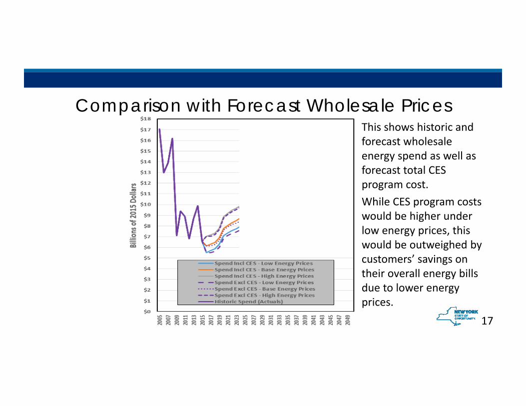
Comparison with Forecast Wholesale Prices

17

This shows historic and forecast wholesale energy spend as well as forecast total CES program cost.While CES program costs would be higher under low energy prices, this would be outweighed by customers’ savings on their overall energy bills due to lower energy prices.

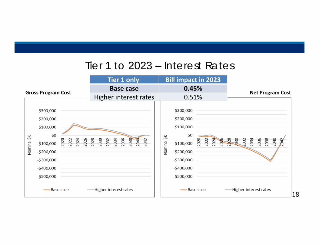
Tier 1 to 2023 – Interest Rates


Tier 1 only Bill impact in 2023Base case 0.45%

Higher interest rates 0.51%

18

Tier 1 to 2023 – Wind Power Cost Sensitivity

19

Base Higher LBW Cost

Tier 1 to 2030 – Technology Cost SensitivitiesTotal CES Tier 1 deployment by 2030

20

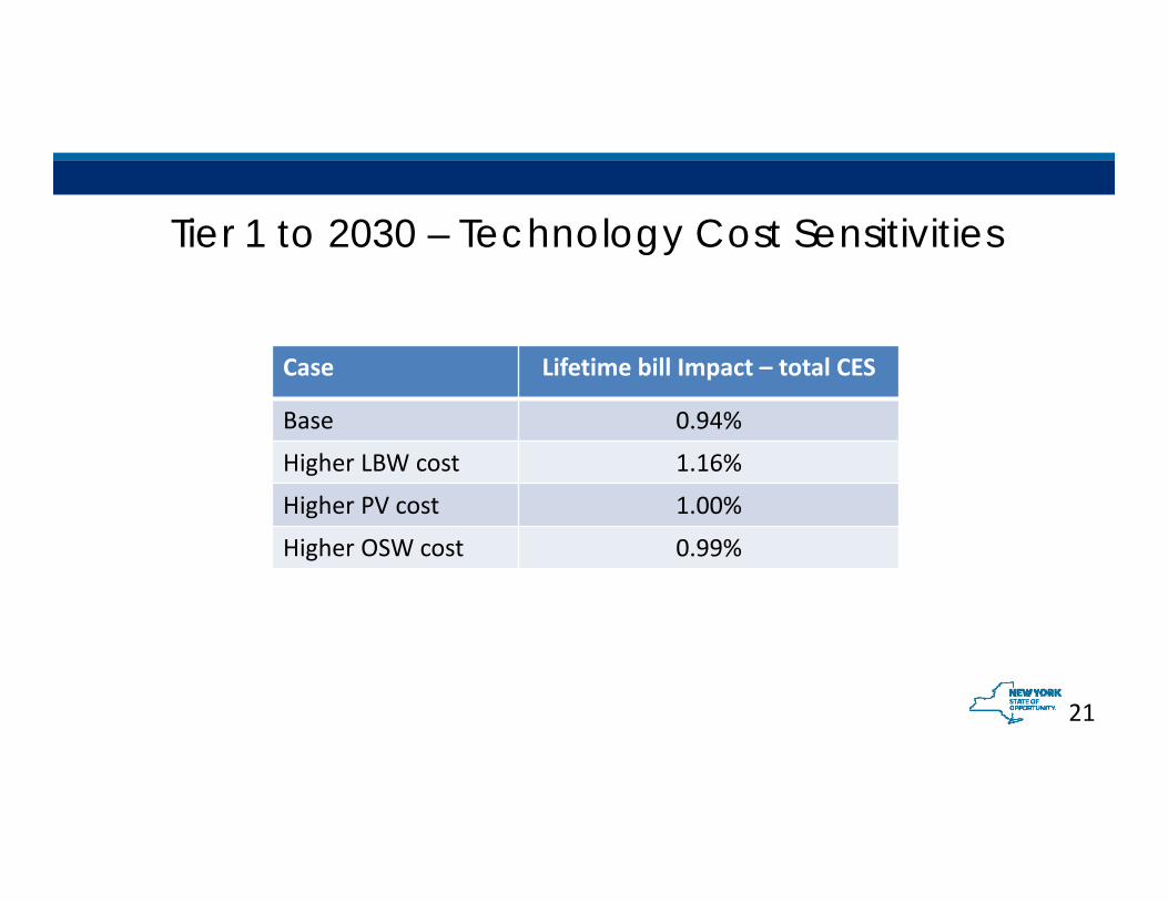
Tier 1 to 2030 – Technology Cost Sensitivities

Case Lifetime bill Impact – total CES

Base 0.94%

Higher LBW cost 1.16%

Higher PV cost 1.00%

Higher OSW cost 0.99%

21

Tier 1 Technology Mix to 2023 – System LoadCapacity ‐ Base Case Capacity ‐ Higher Load

22

Tier 1 to 2023 – System Load


Tier 1 only Bill impact in 2023Base case 0.45%Higher load 0.87%

23

Tier 1 to 2023 – Federal Tax Credits


Tier 1 only Bill impact in 2023Continued tax credits 0.25%

Base case 0.45%No tax credits 0.58%

24

Tier 2A to 2023 – Procurement Structures


Tier 2A only Bill impact in 2023100% PPA 0.30%Base case 0.37%100% spot 0.44%

25

Tier 2A to 2023 – Energy Prices


Tier 2A only Bill impact in 2023100% PPA 0.24%Base case 0.37%100% spot 0.46%

26

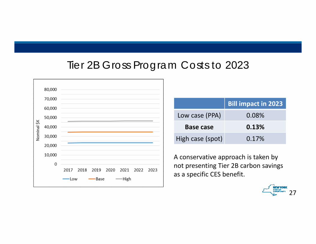
Tier 2B Gross Program Costs to 2023

Bill impact in 2023

Low case (PPA) 0.08%

Base case 0.13%

High case (spot) 0.17%

A conservative approach is taken by not presenting Tier 2B carbon savings as a specific CES benefit.

27

• Goal is to maintain a largely carbon‐free emission source – Benefits include carbon emission reduction, economic impacts, fuel diversity

– “Bridge” to a future where renewables make up a substantially higher percentage of the generation mix

• Quantity of Zero Emission Credits (ZECs) targets will need to be decided

– Clean Energy Standard Staff White Paper proposed a phase‐in approach, starting on 4/1/17

– Other possible approaches can be considered

28

Tier 3

• ZEC Alternative Compliance Payment (ACP) – Setting a price cap due to market power concerns

– To be administratively determined, based on expected revenues and expenses of qualifying facilities

• Costs will have to be filed by prospective ZEC sellers– Confidentiality of data

– Clean Energy Standard Cost Study made certain cost assumptions, but were just illustrative based upon known Ginna plant costs

• Revenue forecasts will have to be made– Clean Energy Standard Cost Study assumed three possible levels of wholesale electric prices in order to

estimate each Tiers’ costs

– Revenue forecast for ZEC ACP calculation will likely be made on a relatively short‐term basis, based on publicly available data

29

Tier 3, cont’d

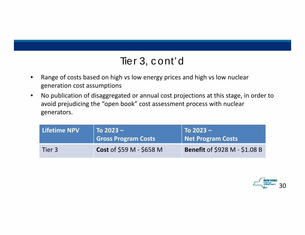
Tier 3, cont’d

Lifetime NPV To 2023 –Gross Program Costs

To 2023 –Net Program Costs

Tier 3 Cost of $59 M ‐ $658 M Benefit of $928 M ‐ $1.08 B

• Range of costs based on high vs low energy prices and high vs low nuclear generation cost assumptions

• No publication of disaggregated or annual cost projections at this stage, in order to avoid prejudicing the “open book” cost assessment process with nuclear generators.

30

Clean Energy Standard Cost StudyMethodology & Assumptions

Bob GraceSustainable Energy Advantage, LLCMay 4, 2016

32

MethodologyTier 1 Modeling OverviewEnergy and Capacity Market ValueFinancing Federal IncentivesTransmission and InterconnectionTier 2 Modeling

33

Tier 1 Modeling Overview

Supply Curve Analysis: Overview• Supply Curve characterizes costs, MW quantity of newly

constructed LSRs available to meet annual incremental demand in NY under long‐term contracts with either:

• Fixed‐price REC contract ($/MWh), or

• Bundled PPA ($/MWh): fixed payment for RECs, energy and capacity

• Supply sources sorted from low to high premium btw. levelized cost of energy (LCOE) and levelized projected commodity market value

• Results derived as all fixed‐price REC, all bundled PPA, or a mix derived by blending (averaging) the results.

34

Team:Sustainable Energy Advantage, LLC (SEA), with input data & resource assumption contributions from:• AWS Truepower

(wind)• Antares Group

(biomass)• Daymark Energy

Advisors (imports)

Cost Elements:Capital Cost; O&M

Cost; Interconnection

Cost; Transmission & Integration Cost;

Financing; Incentives

Renewable LCOE by Zone

Market Commodity Revenues:Energy Price; Capacity PriceRenewable Generation

Premium by Resource Block

Block Clearing Analysis

Incremental LSR Demand to be Met by Supply

Curve

Annual Phase‐In

Differential

Policy Costs

Procured Quantity (MWh and GWh) by Resource by Zone

Procurement Contract Rate

(Levelized Premium for Unbundled;

LCOE for Bundled)

g

Option 1:Clearing Price

Marginal

Option 2:Hybrid Price by Resource Block

Option 3:As‐Bid Price by Resource Block

Supply Curve of Incremental Renewable Supply

2017 to 2030

LSR Model Flow Chart

35

LSR Supply Curve: Key Analysis Parameters• Resource Types characterized:

• Meet RPS Main Tier eligibility criteria and• Most likely to contribute: wind (LBW, OSW); utility‐scale solar; small hydro; biomass

• Geography: • Assumed Eligible: Within New York State + Imports from adjacent control areas with

energy delivered to NY, capacity not committed elsewhere • Analysis includes: PJM (wind), Ontario (wind and small hydro) Quebec (wind) available to

and deliverable to NYISO; New England ignored (net importer from NY)

• Temporal Factors• Each project assumed contracted for 20 yrs• Analysis horizon: start of commercial operation from 2017 – 2030• Policy payments for production in 2017 ‐ 2049 when last of 20‐year contracts expire

36

Assumed Lag from Contract to Operation

37

• Rounded to nearest full year in model

Key Characteristics of Resource BlocksLocation

(NYISO zone) Developable

Quantity (in MW) Capacity Factor (%) “Typical” Scale (MW)

Capital Expenditures

(CAPEX) incl. T&I ($/kW)

Cost of Network Upgrades

Fixed & Variable O&M (or OPEX)

Costs Production Profile

Carrying charge (financing costs & structure) (% of

CAPEX)

IncentivesHeat Rate & Fuel Cost

(for biomass)

CAPEX may include:

– Installed costs of generator hardware

– Interconnection costs

– Labor

– Reserves

– Financing‐related transaction costs

O&M may include:

– Cost of labor and parts

– Insurance

– Land costs (leases, royalties, etc.)

– Management and administrative fees

– Taxes or payments in lieu of tax (PILOTS)

– Capital replacements and overhauls

Cost of capital, capital structure,

financing requirements

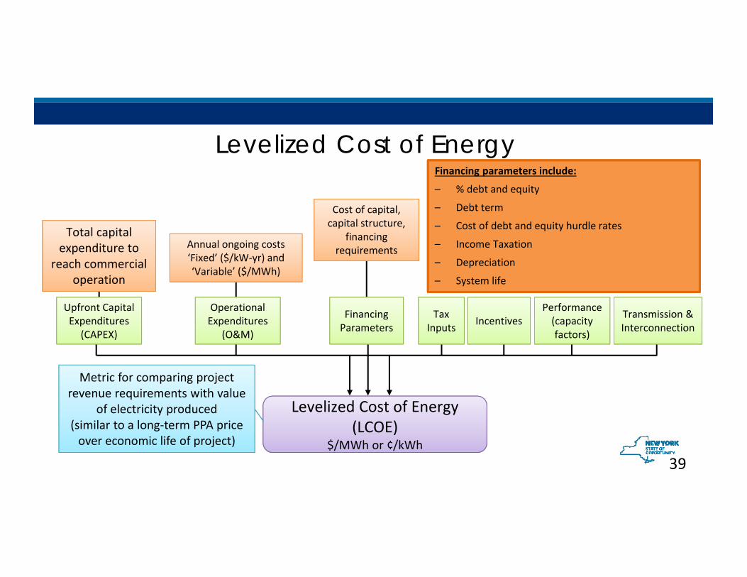
Levelized Cost of Energy

39

Upfront Capital Expenditures

(CAPEX)

Operational Expenditures

(O&M)

Financing Parameters

Performance (capacity factors)

Transmission & InterconnectionIncentivesTax

Inputs

Total capital expenditure to

reach commercial operation

Annual ongoing costs ‘Fixed’ ($/kW‐yr) and ‘Variable’ ($/MWh)

Levelized Cost of Energy (LCOE)

$/MWh or ¢/kWh

Metric for comparing project revenue requirements with value

of electricity produced(similar to a long‐term PPA price over economic life of project)

Financing parameters include:

– % debt and equity

– Debt term

– Cost of debt and equity hurdle rates

– Income Taxation

– Depreciation

– System life

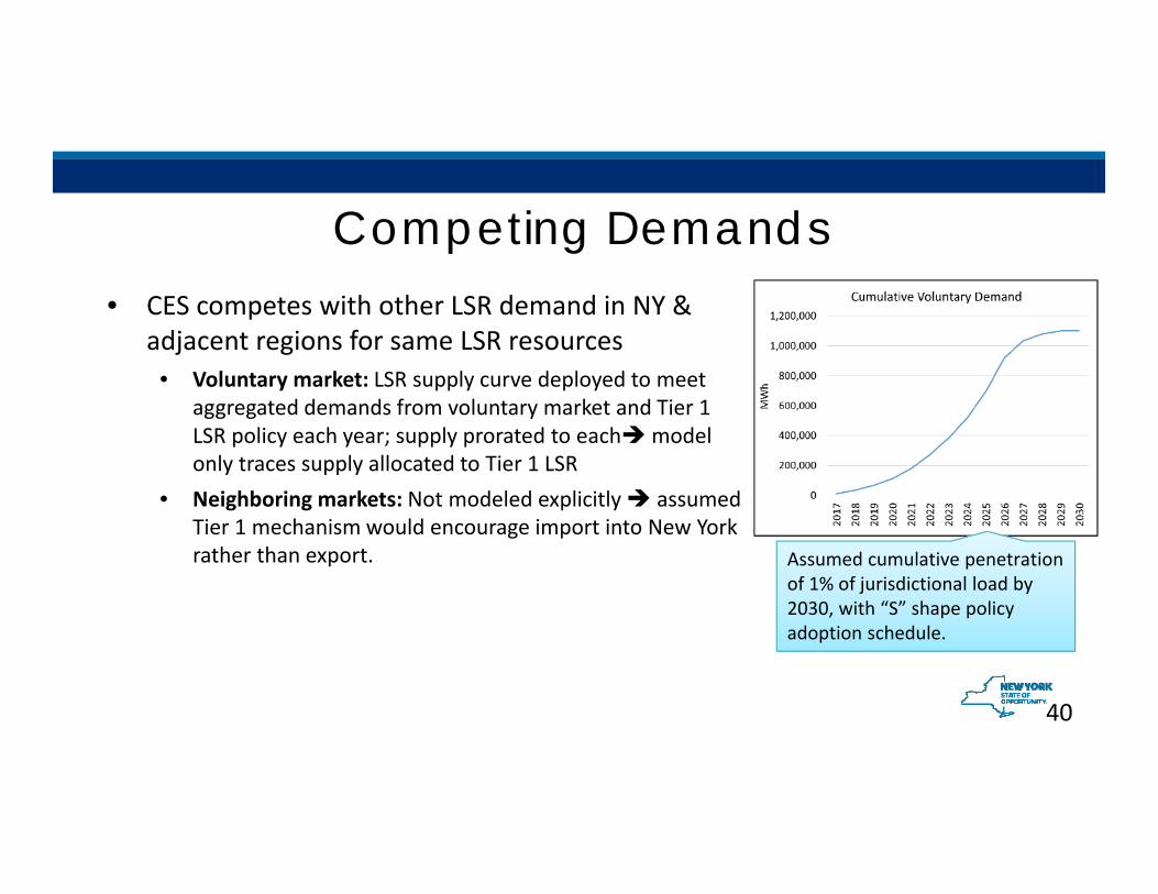
Competing Demands• CES competes with other LSR demand in NY &

adjacent regions for same LSR resources • Voluntary market: LSR supply curve deployed to meet

aggregated demands from voluntary market and Tier 1 LSR policy each year; supply prorated to eachmodel only traces supply allocated to Tier 1 LSR

• Neighboring markets: Not modeled explicitly assumed Tier 1 mechanism would encourage import into New York rather than export.

40

Assumed cumulative penetration of 1% of jurisdictional load by 2030, with “S” shape policy adoption schedule.

Net Program Costs Reflect Carbon Value ($/MWh)

41

• Avoided marginal CO2 emission rate ~ 1,077 pounds (0.538 short tons) per MWh1

• Net program costs = gross program costs less Incremental Social Carbon Benefit

Total social cost of carbon taken from EPA’s

July 2015 revised Technical Update.

Pecuniary value of CO taken

p

Pecuniary value of CO2 taken from 2015 NYISO CARIS

forecast of RGGI allowance prices.

Incremental Incremental Social Carbon Benefit

42

Energy and Capacity Market Value

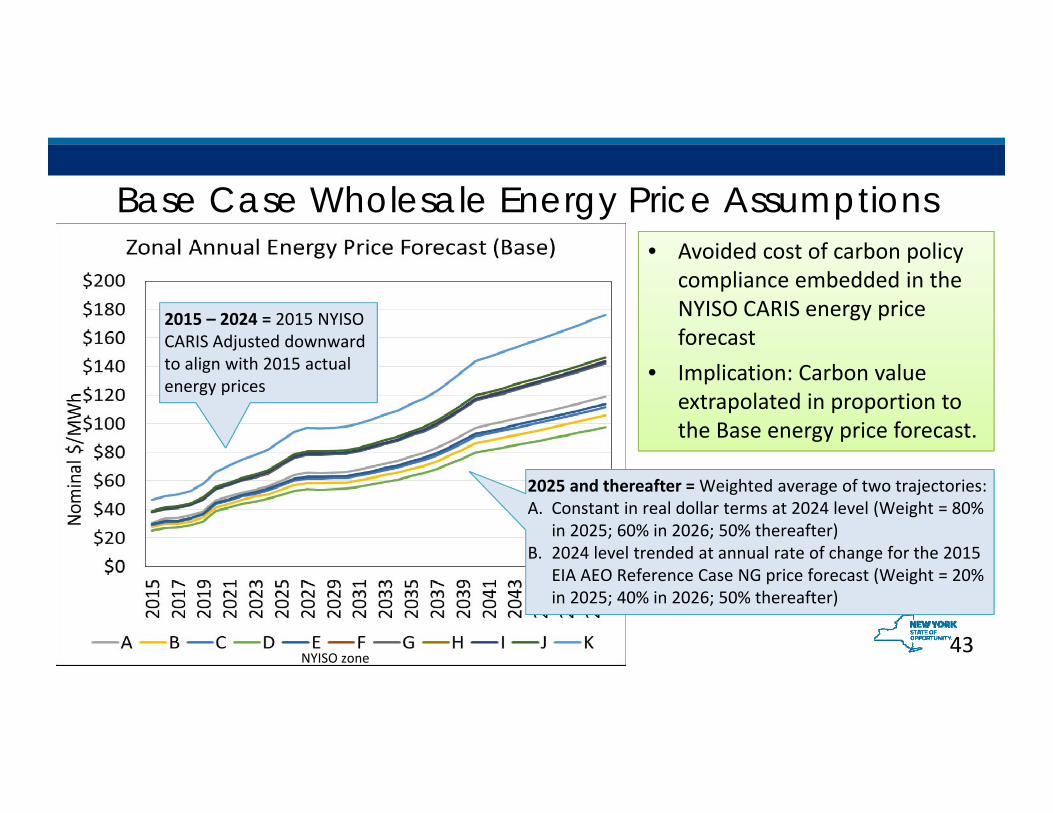
Base Case Wholesale Energy Price Assumptions• Avoided cost of carbon policy

compliance embedded in the NYISO CARIS energy price forecast

• Implication: Carbon value extrapolated in proportion to the Base energy price forecast.

2025 and thereafter = Weighted average of two trajectories:A. Constant in real dollar terms at 2024 level (Weight = 80%

in 2025; 60% in 2026; 50% thereafter)B. 2024 level trended at annual rate of change for the 2015

EIA AEO Reference Case NG price forecast (Weight = 20% in 2025; 40% in 2026; 50% thereafter)

2015 – 2024 = 2015 NYISO CARIS Adjusted downward to align with 2015 actual energy prices

43NYISO zone

Low: 90% of Base Case Low: 90% of Base Case Prices at all time

High: 115% of Base Case Prices at all time

Alternative energy market price futures to test sensitivity of program costs to market values

44

Capacity Price Forecast

ICAP zone:

45

2015 – 2035: per BCA

BCA = Order Establishing the Benefit Cost Analysis Framework, Case 14‐M‐0101, January 21, 2016

Thereafter:held constant in real

terms

BCA’s Zonal Summer and Winter ICAP generator prices translated to zonal average annual UCAP prices using average of zonal Summer 2015 and Winter 2015/16 translation factors

46

Financing

Financing Assumption Framework

• The differing risk exposure under different contracting and incentive regimes is reflected solely through differences in the cost of capital

• (revenue streams are not discounted from the forecasts to reflect risk)

• Financing assumptions calibrated against available benchmark data from outside NYS and data from past Main Tier solicitations in NY.

Financing Assumptions: Debt % and Term

48

Remainder sourced from equity.

Additional Assumptions: 20‐yr contract duration35% Federal, 7.1% NYS tax rate

***

*

* = PTC or ITC as applicable

Financing Assumptions: Cost of Equity & Debt

49

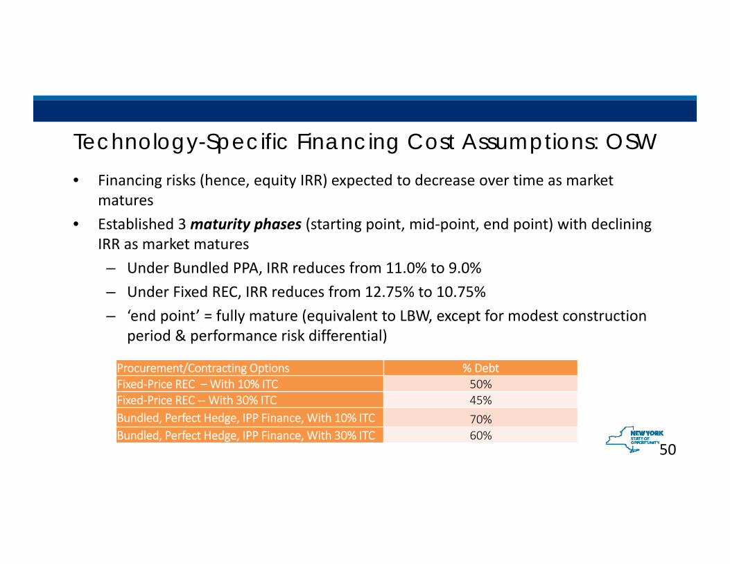
Technology-Specific Financing Cost Assumptions: OSW• Financing risks (hence, equity IRR) expected to decrease over time as market

matures• Established 3 maturity phases (starting point, mid‐point, end point) with declining

IRR as market matures– Under Bundled PPA, IRR reduces from 11.0% to 9.0%– Under Fixed REC, IRR reduces from 12.75% to 10.75%– ‘end point’ = fully mature (equivalent to LBW, except for modest construction

period & performance risk differential)

50

Procurement/Contracting Options % DebtFixed‐Price REC – With 10% ITC 50%Fixed‐Price REC ‐‐With 30% ITC 45%Bundled, Perfect Hedge, IPP Finance, With 10% ITC 70%Bundled, Perfect Hedge, IPP Finance, With 30% ITC 60%

51

Federal Incentives

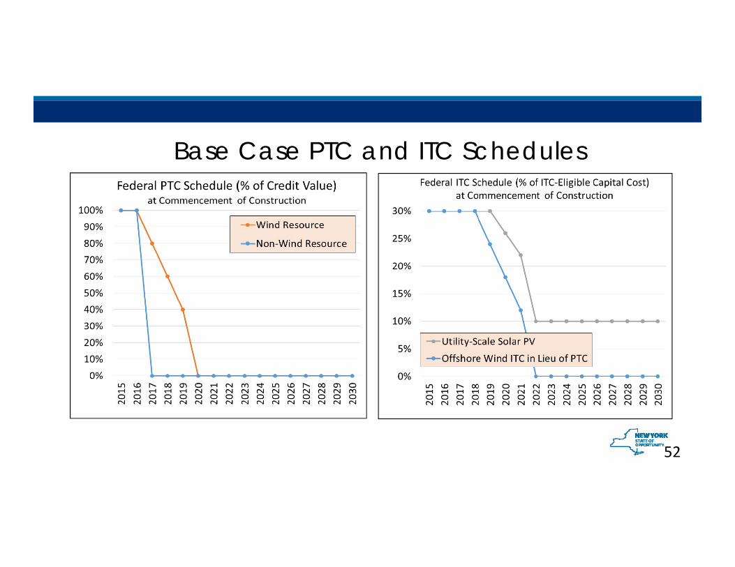
Base Case PTC and ITC Schedules

52

Increased scarcity of tax equity assumed investors unable to fully monetize value of tax credits

TechnologyEquivalent % of Tax Credit Value Effectively Monetized

LBW (10‐30 MW) 80.0%LBW (30‐100 MW) 90.0%LBW (100‐200 MW) (>200 MW) 90.0%Utility‐Scale Solar PV 90.0%Hydro (Upgrades) 75.0%Hydro (NPD) 75.0%Woody Biomass 75.0%Biogas 75.0%Offshore Wind 90.0%

53

Value of FTC reduced to the percentage of ‘face value.’

54

Transmission and Interconnection

Transmission & Interconnection (T&I) Costs

“Extension Cord” (generator lead costs): Interconnect to existing transmission system included in CAPEX modeled as sum of:

• New generator lead line: miles * voltage‐specific $/mi• “non‐line” cost of interconnecting to via new or existing substation, e.g. cost

of building new substation, expanding existing substation, installing new breaker & other equipment

Transmission & Interconnection (T&I) Costs

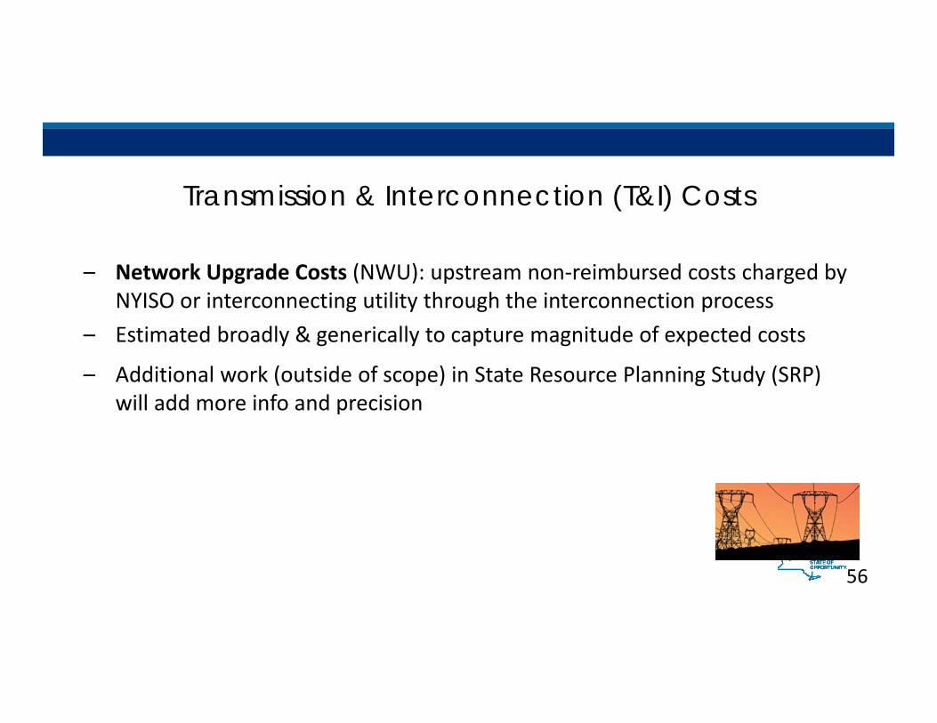
– Network Upgrade Costs (NWU): upstream non‐reimbursed costs charged by NYISO or interconnecting utility through the interconnection process

– Estimated broadly & generically to capture magnitude of expected costs

– Additional work (outside of scope) in State Resource Planning Study (SRP) will add more info and precision

56

57

Tier 2 Modeling Overview

Tier 2A Approach• By definition, have material revenue opportunities in surrounding markets

• Historically: New England spot Class I REC prices, if energy delivered to ISO-NE• In the future, PJM ‘Tier 1’ RPS markets could become competitively attractive.

• Objective: retain energy (GHG impact) & RECs (CES targets) in NY thru 2030

• Targets:• Large hydro not eligible• Initial: contribution of eligible resources to 2014 baseline (i.e., generation of such

resources net of exports at that time)• Increase as Main Tier RPS contracts end

• What revenues would successfully attract such resources to sell their RECs in New York State rather than exporting their energy to other markets?• Cost estimates based on assessment of generator’s opportunity cost

58

59Tier 2A: Spot vs. Bundled PPASpot

• Analysis based on NY market providing a similar or slightly lower level of revenue risk as spot prices available in alternative markets

• Assumed: Alternative Compliance Payment is set as a cap on spot REC prices; Tier 2A cost estimate based on cap

PPA• Analysis based on NY bundled

PPA revenue stream providing necessary incentive for generation to stay in New York State at a lower expected cost due to the added revenue certainty/lower risk

• Assumed duration from year generation first becomes eligible through 2030 (i.e., progressively decreasing contract duration)

Risks & rewards differ expected revenue streams valued differently59

Tier 2B Resources Have Limited REC Revenue Opportunities

• Generally older renewable electricity generators with limited alternative revenue opportunities (not ‘Class I’ eligible)

• Generally lower than cost of accessing them

• Objectives: retain energy (GHG impact) & RECs (CES targets) in NY thru 2030, acquire rights to count them, and keep projects from shutting down

• Targets: set based on amount of LSR in the 2014 baseline not owned by NY State Entities, net of expired RPS Main tier contracts.

• What revenues would successfully cause resources to sell their RECs in NY?– Costs estimated based on representative pricing levels observed for comparable resources

in Northeast RPS programs. – Assumed sufficiently above transactions costs to motivate sale of RECs to CES obligated

entities (but not much more)6060

61

Tier 1Technology Specific Methodology & Assumptions

Land‐Based Wind Offshore WindUtility‐Scale Solar PVImportsSmall HydroelectricWoody BiomassBiogas

62

Land-Based Wind

Overview of Approach

• Detailed geospatial approach identifies candidate windy sites• Reflects site‐specific nature of LBW resource potential, production, project cost,

and interconnection cost• Raw potential derated to reflect varying likelihood of permitting success• Cost functions used to represent development cost variations associated with site

characteristics.

Land-based Wind

63

LBW Capital Expenditures (excluding T&I Costs)• Starting CAPEX (2015 NREL ATB) = $1,692/kW (in 2013 $); for 200‐MW project in

idealized central US plains 3 multiplicative adjustments applied to starting point to reflect cost characteristics specific to each LBW site:

Land-based Wind

64

NY Region NYISO Zones EIA Regional Factor Siting Factor Final Adjustment FactorUpstate Rest of state 1.01 1.06 1.07NYC Zone J N/A N/A N/ALI Zone K 1.25 1.10 1.38

Technology Size Category Adjustment FactorLBW 10‐30 MW 1.30LBW 30‐100 MW 1.15LBW 10‐30 MW 1.02LBW >200 MW 1

Land Type Definition Min. Elevation (m)

Min. Elevation Difference vs. Surroundings (m)

AdjustmentFactor

Plain 1 Slope = 0 – 5%, Not 3 or 4 N/A N/A 1.00Rolling Hills (Accessible) 2 Slope = >5 – 15%, Not 1,3 or 4 N/A N/A 1.07Rolling Hills (Remote) 3 Slope = 8 – 12%, Not 4 300 100 1.12Mountainous 4 Slope = >10 – 20% 500 N/A 1.22

Locational adjustments:

Reflects difference btw. national average and costs specific to Upstate NY and Long Island

Size adjustment: reflects diseconomy of scale in size categories smaller than 200 MW baselineReflects siting & soft cost difference

from idealized (central plains) site

Topography adjustment: reflects cost differences in site topography (slopes) and access to roads.

LBW CAPEX Experience Curve Index• Derived by indexing Mid NREL ATB

CAPEX forecasts for NREL’s ‘techno‐resource group’ (TRG) 2.

• TRGs 2 and 3 most consistent with conditions with majority of sites in New York.

• Projected rates of cost decline slower than the rate of inflation LBW CAPEX increases over time in nominal dollars

Land-based Wind

65

Geospatial LBW Resource Potential AnalysisLBW Primary and Secondary Constraints

Land-based Wind

• Primary constraint areas excluded from analysis • Model can apply probability de‐rates to sites

intersecting secondary constraint areas to represent a higher hurdle to permitting success (not applied in analysis):

• Department of Defense Lands• Forest Service lands• State forest lands• Modeled rare species distributions• Modeled migratory bird stopovers• Bat distributions/locations/travel zones• Terrestrial connectivity and resilience

66

Primary Constraints ‐ Excluded Areas BufferAdirondack and Catskill Parks 100 ft.National Historic Preserves / Sites / Parks 100 ft.Wildlife Management Areas 100 ft.State Unique Area 100 ft.State and Local Parks 100 ft.National Monuments 100 ft.National Wildlife Refuges 100 ft.National Park Service Land 100 ft.Fish and Wildlife Service Lands 100 ft.American Indian Lands 100 ft.GAP Status 1 & 2 Lands (Protected Lands) 100 ft.

Urban AreasClass (22) – 200 m;

Class (23) & (24) – 500 mWetlands & Waterbodies 100 ft.Large Airports 20,000 ft.Small / Medium Airports 10,000 ft.Proposed Wind Farms 3 kmExisting Wind Farms 3 kmSlopes > 20% N/AAppalachian Trail 3 km

LBW Sites• Continuous areas capable of hosting a wind project >10 MW

• Land area and power density (measured in MW/km2) consistent with topography • Wind speeds at 4 hub heights (80m, 100m, 120m and 140m)• Average slope and elevation• Distance to nearest existing transmission lines and substations at 5 voltages

• Manual site characterization to assess potential siting conflicts due to presence or proximity of dwellings/roads at individual sites:

• Sites with “substantial” housing density excluded outright• % de‐rates applied to reduce the available land areas associated with 4 levels of housing densities:

• High: 95% (i.e., only 5% of the land area developable)• Medium: 75%• Low: 30%• None: 5%

Land-based Wind

67

Distribution of Potential LBW Sites(370 New York LBW Sites in the Supply Curve)

Land-based Wind

NOTE: This is the result of probabilistic geospatial analysis and should not be interpreted as defining actual project sites. 68

LBW Capacity Factors• Capacity factors modeled at four hub heights (80m, 100m, 120m and

140m) using scalable wind turbine power curve representing current, commercially‐available technology

• Hub heights (HH) used as a proxy for a combination of blade length (rotor swept area) and HH for determining capacity factors at any given wind regime assumed to continue recent increasing trend over span of study.

• Evolution of capacity factors over time was modeled based on two parameters:• Average fleet hub height evolution; and• Technology advancement at a constant hub height.

Land-based Wind

69

LBW Technology Advancement Factors(Additional technology improvement, represented by c.f. at a given HH)

• Derived from 2015 NREL ATB mid and low trends for TRG 3

• Reduced NREL ATB rate of change figures by 50% to eliminate potential double counting of impact driven by HH increase

Land-based Wind

70

LCOE Supply Curves: LBW 30-100 MWLand-based Wind

71

Phase‐out of PTC

Inflation outpaces experience

curve

72

Offshore Wind

OSW Data and Methodology • OSW analysis builds on:

• March 2016 Massachusetts Offshore Wind Future Cost Study• 2015 NREL ATB• Earlier NYSERDA‐internal analysis

• Starting point from NYSERDA‐internal cost & resource analysis adjusted/extrapolated using SIOW 2016 Massachusetts Study, NREL ATB to reflect confluence of several factors:

• Latest European experience in cost reduction;• Scale economies and industrialization of OSW sector (global learning)• Continued scaling from 5 MW to 8 MW class turbines • U.S. learning and industry scaling• Availability of long‐term revenue certainty• Increased competition consistent w/ eastern US commitment to deploy OSW at scale thru 2030 • Development of domestic supply chain, spreading of fixed costs

Offshore Wind

73

Offshore Site

Area (km2)

Build‐Out Potential (MW)

MW Assumed Available

before 2030 (MW)

1 285 855 7912 663 1,989 12953 1,521 4,563 25945 1,372 4,116 24026 1,027 3,081 1869

OSW Resource PotentialInterconnection

Points

Offshore Wind

Of 6 potential offshore wind areas characterized, 5 were selected as the closest, most advanced and/or most representative of the resource potential reasonably available

during the Study period.

Figure A.8 74

1

5

2

3

6

OSW CAPEX Trajectory

75

‘2015 NREL ATB CAPEX trajectory’:developed using 2015 NREL ATB CAPEX (Mid) trajectory, TRG 5/6.

‘2015 NREL ATB CAPEX trajectory’:developed using 2015 NREL ATB CAPEX (Mid) trajectory, TRG 5/6.

From 2023 onward, this forecast trajectory increases in nominal terms too conservative.

From 2023 onward, this forecast trajectory increases in nominal terms too conservative.

‘2016 SIOW CAPEX trajectory’: developed from trending OSW tranches A, B, &C in 2016 SIOW analysis.

‘2016 SIOW CAPEX trajectory’: developed from trending OSW tranches A, B, &C in 2016 SIOW analysis.

Base case trajectory: NY Site‐specific CAPEX from NYSERDA‐internal analysis, trended until 2023 at ‘2015 NREL ATB CAPEX’ trajectory, trended thereafter @ 2016 SIOW CAPEX trajectory

Base case trajectory: NY Site‐specific CAPEX from NYSERDA‐internal analysis, trended until 2023 at ‘2015 NREL ATB CAPEX’ trajectory, trended thereafter @ 2016 SIOW CAPEX trajectory

Alternative high cost OSW CAPEX trajectory: 2023 base case starting point, trended to hybrid learning curve index based on a weighting of ‘2015 NREL ATB CAPEX trajectory’ index (30% weight) & ‘2016 SIOW CAPEX trajectory’ index (70% weight).

Alternative high cost OSW CAPEX trajectory: 2023 base case starting point, trended to hybrid learning curve index based on a weighting of ‘2015 NREL ATB CAPEX trajectory’ index (30% weight) & ‘2016 SIOW CAPEX trajectory’ index (70% weight).

OSW T&I Costs• T&I costs for ERIS from NYSERDA‐internal analysis used, but OSW projects assumed

able to access capacity revenue.

• In deriving T&I estimates, the following key assumptions were made:

• Most of distance between OSW project & onshore interconnection point via undersea cable

• Fraction of T&I costs associated with onshore facilities assumed owned by interconnecting utility and charged back to project owner (at lower cost of capital), while remainder assumed to be financed by project owner at same capital structure as generation facilities.

• T&I costs held constant in real $ through 2020; thereafter, assumed annual decrease by 1% in real $ through 2030

Offshore Wind

76

Technological AdvancementOffshore Wind

77

The starting points were trended with a technological advance index developed by first taking the average of the c.f. trajectories (Mid) for TRG 5 and TRG 6 in the 2015 NREL ATB, then converting the trajectory into an index with 2017 as the base.

Net c.f.s were applied to a composite power curve for an 8‐MW wind turbine.

The 2017 c.f.s for each site, modeled by AWST, are as follows:• Site 1 – 43.6%• Site 2 – 44.01%• Site 3 – 44.83%• Sites 5 & 6 – 44.52%

CAPEX and OPEX figures reflect technology evolution which includes both larger turbines at higher hub heights, and other technology advances.

LCOE Supply Curves – Offshore WindOffshore Wind

Rapid increase in resource availability in later years due to market maturation.

78

Global cost reductions & scale economies

associated w/ market visibility

79

Utility-Scale Solar PV

Utility Scale Solar Photovoltaic (PV): Overview of Approach

• Analysis focused on 10‐30 MW installations assumed most likely

• Geospatial analysis estimated total developable area • PV has homogenous costs (other than interconnection) and

production resource blocks aggregated by similar cost characteristics within each NYISO zone


80

• Baseline CAPEX based on publicly available sources, recent LSR analyses, and interviews with solar developers active (or planning to be active in this scale) in NY

• Locational adjustments applied to the Baselines:

• The capacity & $/kW cost data (CAPEX & Fixed O&M) used are expressed in DC.


Utility-Scale Solar PV CAPEX (Not Including T&I Cost)

81

CAPEX Baseline (2014$/kWDC) 2014 CAPEX BaselineTechnology & Size Category Base ConservativeSolar 10‐30 MW, Fixed Tilt $1,423 $1,503Solar 10‐30 MW, Single Axis $1,843 $1,843

Utility‐Scale PV CAPEX Baseline Assumes a lower degree of market maturation; used for the High PV Cost sensitivity scenario.

NY Region NYISO ZonesEIA Regional

FactorSiting Factor

Final Adjustment Factor

Upstate A, thru I 0.98 1.00 0.98NYC J 1.25 1.02 1.28LI K 1.45 1.02 1.48

Utility‐Scale PV CAPEX Adjustment FactorsReflects cost differences of solar siting and permitting between different NY regions and the national average.

Reflects regional cost differences in PV development among NY regions

EIA Regional Factor * Siting Factor

(1) Greentech Media November 3, 2015 Presentation (http://www.greentechmedia.com/articles/read/Slideshow‐Reaching‐250‐GW‐The‐Next‐Order‐of‐Magnitude‐in‐US‐Solar)

Utility-Scale Solar PV Fixed-Tilt Cost TrendUtility-Scale Solar PV

‘GTM – Adjusted Post 2020’: ‘GTM Base’ forecast through 2020; thereafter, assumes cost trajectory declines by 1.0%/yrnominal; used in all but ‘High PV Cost Sensitivity’ scenario.

Graph shows relative cost change compared to start year

82

‘GTM Base’: CAPEX trajectory developed using cost trend published by Greentech Media in November 20151; used through 2030 for ‘High PV Cost Sensitivity’ scenario.

Geospatial Utility-Scale Solar Resource Potential AnalysisPrimary Constraints ‐ Excluded Areas

Additional Buffer Beyond Excluded Area

Adirondack and Catskill Parks 100 ft.National Historic Preserves/Sites/Parks 100 ft.Wildlife Management Areas 100 ft.State Unique Area 100 ft.State and Local Parks 100 ft.National Monuments 100 ft.National Wildlife Refuges 100 ft.National Park Service Land 100 ft.Fish and Wildlife Service Lands 100 ft.American Indian Lands 100 ft.GAP Status 1 & 2 Lands (Protected Lands) 100 ft.Urban Areas 25 ft.Forests 0 ft.Cultivated Crops 0 ft.Wetlands & Waterbodies 100 ft.Existing Roads and Highways 25 ft.Airports 25 ft.Slopes ≥ 5% N/A

• Primary constraint land areas excluded

• Excluded areas ≥ 2 miles of any roads, ≥3 miles of any existing substations

• Sites requiring interconnection to new substations not considered

• Site resource potential = Site area * Power Density; Power density = 7.5 acres/MW

• Remaining contiguous areas capable of hosting projects ≥ 10 MW considered as potential project sites.


83

**

Probability De-rates by Land Cover TypeUtility-Scale Solar PV

• Project sites correlated with:• Barren Land• Shrub/Scrub• Grassland/Herbaceous• Pasture/Hay

• Only allowed for solar deployment on 25% of ‘pasture/hay’ area within a site to reflect competing uses

84Potential sites shown are result of probabilistic geospatial analysis, should not be interpreted as defining actual project sites

Capacity Factors

• Year 1 c.f.s derived using PV Watts® at representative NYISO zone based on assumed system characteristics

• Annual production levelized to account for annual production degradation of 0.5%.

Zone Selected Location Fixed 1‐AxisA Buffalo 13.7% 16.2%B Rochester 13.9% 16.5%C Syracuse 14.2% 17.0%D Plattsburgh 14.6% 17.3%E Utica 12.7% 15.1%F Albany 14.6% 17.3%G Poughkeepsie 13.3% 15.7%H Millwood 14.4% 17.2%I Yonkers 15.1% 18.1%J New York City 15.4% 18.3%K Long Island 14.7% 17.6%


Year 1 PV capacity factors (at DC rating) by zone

85

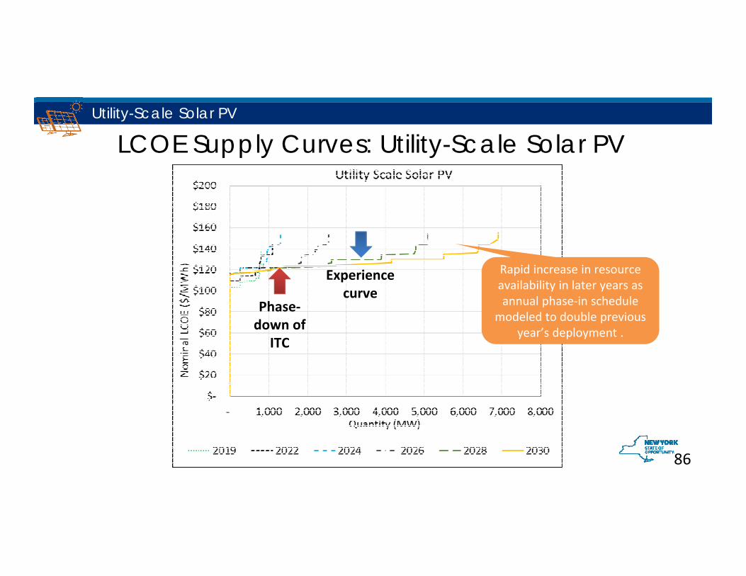
LCOE Supply Curves: Utility-Scale Solar PV

Rapid increase in resource availability in later years as annual phase‐in schedule

modeled to double previous year’s deployment .


86

Experience curve

Phase‐down of

ITC

87

Imports

Overview of Approach to LSR Imports• Resources from adjacent control areas capable of delivering to NY considered

simplified modeling approach• Focused on resources most likely to export to NY • Physical transmission inter‐ties, competing usage of ties & available space on ties

used to estimate assumed practical transfer limits for PPA supply• Competing native demands and internal transmission constraints in neighboring

control areas limit export to NY. • Additional factors considered in characterizing LSR imports:

• NYISO delivery zone • Potential transaction cost & risks of export/import transaction• Electrical losses• Potential loss of ability to monetize capacity revenue in exporting market or NYISO

88

Imports

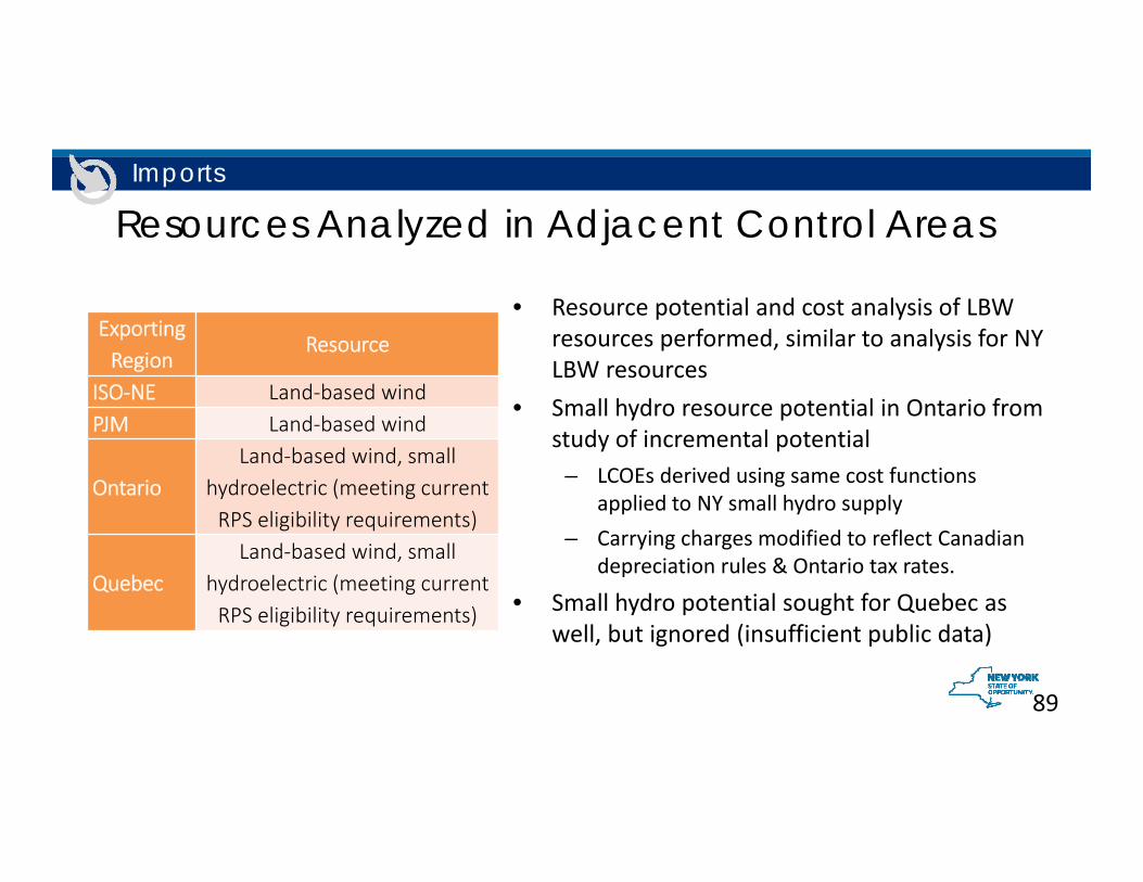
Resources Analyzed in Adjacent Control Areas

Exporting Region

Resource

ISO‐NE Land‐based windPJM Land‐based wind

OntarioLand‐based wind, small

hydroelectric (meeting current RPS eligibility requirements)

QuebecLand‐based wind, small

hydroelectric (meeting current RPS eligibility requirements)

• Resource potential and cost analysis of LBW resources performed, similar to analysis for NY LBW resources

• Small hydro resource potential in Ontario from study of incremental potential

– LCOEs derived using same cost functions applied to NY small hydro supply

– Carrying charges modified to reflect Canadian depreciation rules & Ontario tax rates.

• Small hydro potential sought for Quebec as well, but ignored (insufficient public data)

89

Imports

Constraints on Out-of-State Resources for CES Tier 1 Supply Curve

• Portion of eastern PJM states’ RPS demands assumed met first from supply• Wind supply from Ohio westward assumed inaccessible (or too costly) to NY

due to west‐to‐east transmission constraints• Ontario procurement policy demands assumed met first from supply• Supply from northern and western Ontario limited by material internal

transmission constraints, further blocked from getting through Toronto area• New England LSR supply excluded (strong demands, substantial current &

proposed flow of supply from NY to New England)

Imports

90

91MW Available over NY Interties at least 85% of hours per year

ISONE‐NYISO

NPX‐1385 NPX‐CSC HQ‐

NYISOHQ‐

CedarsIMO‐NYISO

PJM Neptune

PJM NYISO

SCH‐HQ Import Export

SCH PJM VFT

SCH PJM HTP

2014 950 8 ‐ ‐ ‐ 453 ‐ 1,460 5 65 360

2015 1,128 30 ‐ ‐ ‐ 516 ‐ 1,311 ‐ ‐ 460

Average 1,039 19 ‐ ‐ ‐ 485 ‐ 1,385 3 33 410

MW available for at least 85% of hours in year, based on 2014‐2015 usage, assumed practical limit to imports.

91

Imports

92Key Import Analysis Assumptions

Source Market Interface

Assumed NYISO Delivery Zone

Assume Practical Transfer Limit for

PPA Supply (MW)

Market Adjustment Factor

Assumed Max

Imports (MW)

Cost of Importing Power (2015

$/MWh)

Losses(to the extent

applied outside of LMP pricing)

(%)

Incremental Native Demand (MW)

ISO‐NE ISONE‐NYISO F 1,039.2 0% ‐ $ 1.30 0.0% all NPX‐1385 K 19.0 0% ‐ 0.0% all NPX‐CSC K ‐ 0% ‐ 0.0% all

Quebec (HQ) HQ‐NYISO D ‐ 0% ‐ $12.50 ? 0HQ‐Cedars D ‐ 0% ‐ $12.50 ? 0

Champlain Hudson Power Express F 1,000.0 100% 1,000 $10.20 ?? 0

Ontario (IMO) IMO‐NYISO A 484.8 100% 480 $4.20 ? Yes

PJM PJM Neptune K ‐ 0% ‐ $12.90 ? Eastern

PJM NYISO A, C 1,385.3 100% 1,390 $9.20 0.0% Eastern

SCH PJM VFT J 32.5 0% ‐ $9.20 2.5% Eastern

SCH PJM HTP J 410.0 100% 410 $21.00 1.9% Eastern

Imports

93

Small Hydroelectric

Overview of Approach: Hydro• Costs & resource potential based on:

• literature review of Idaho National Engineering and Environmental Laboratory (INL), Oak Ridge National Laboratory (ORNL), & U.S. Department of Energy

• interviews with developers active in NY hydro market

• Hydro cost characteristics extremely site‐ & size‐sensitive analysis usescentral estimates

• Categories meeting RPS MT eligibility (<30 MW, or no new impoundment) Upgrades of existing generation facilities New generation at Non‐Powered Dams (NPD)• No data available on repowering of existing dams due to lack of public data, despite

some indication of development activities in NY (grouped in INL & ORNL studies?)• Run‐of‐river/in‐stream assumed not commercial before 2030

Small Hydroelectric

94

95

Woody Biomass

Overview of Approach: Incremental Biomass• Resources included:

• Repowered operating/retired fossil‐fueled plants to dedicated biomass‐to‐energy• Greenfield dedicated biomass integrated gasification combined cycle (IGCC)

• Resources excluded:• Direct fire/fluidized bed biomass (unlikely to be permittable or economic) • Co‐firing @ coal‐fired plants (Gov. Cuomo’s intent to retire all NY coal‐fired plants)• New & existing combined heat and power (CHP) (simplification)

Woody Biomass

96

97

Biogas

Overview of Approach• Focused on anaerobic digestion at waste water treatment plants (WWTPs)• other biogas resources assumed eligible for Tier 1 not modeled (high

costs, relatively small quantities, technologies not yet fully commercial)• 34 WWTP facilities with design flows of ≥20 MGD studied (79% of

treatment capacity in NY) facilities at this scale have potential for higher quantities of biogas production larger electric generation capacities

Biogas

98

clean energy standard cost study€¦ · • the clean energy standard cost study complements and...

Documents