cleaning house: the impact of information technology monitoring on employee … · ·...
TRANSCRIPT

Cleaning House: The Impact of Information Technology Monitoring on Employee Theft and Productivity*
Lamar Pierce†
Washington University in St. Louis [email protected]
Daniel Snow
Brigham Young University [email protected]
Andrew McAfee
Massachusetts Institute of Technology [email protected]
August 27, 2013
In this paper, we study how firm investments in technology-based employee monitoring impact both misconduct and productivity. We use unique and detailed theft and sales data from 392 restaurant locations from five different chains that adopt a theft monitoring information technology (IT) product. Since the specific timing of individual locations’ technology adoption is plausibly exogenous, we can use difference-in-differences models to estimate the treatment effect of IT monitoring on theft and productivity within each location for all employees. We find significant treatment effects in reduced theft and improved productivity that appear to be driven by changing the behavior of individual workers rather than selection effects. These findings suggest multitasking by employees under a pay-for-performance system, as they increase effort toward sales following monitoring implementation in order to compensate for lost theft income. In addition to substantial financial benefits to the firms in our sample, the average worker enjoys increased tip-based earnings of $0.58 per hour. Our results suggest that employee misconduct is primarily a result of managerial policies rather than individual differences in ethics or morality, and that policies that reduce misconduct can benefit both firms and employees.
* We thank Bart Hamilton, Ian Larkin, Lars Lefgren, Jason Snyder, and participants in seminars at Harvard Business School, HEC Lausanne, Boston University, Washington University, and BYU for their comments and suggestions on the paper. Jeff Hindman and Scott Walton were critical to acquiring and understanding the data, while Thomas Bennett and John Holbrook provided invaluable research support. † Olin Business School, One Brookings Drive Box 1133, St. Louis MO 63130. [email protected]
I . Introduction
Employee theft and fraud are widespread problems in firms, with workers stealing roughly $200
billion in revenue from U.S. firms to supplement their income (Murphy 1993).1 A growing empirical
literature on forensic economics has clarified when and how theft and other misconduct occur (e.g., Jacob and
Levitt 2003; Fisman and Wei 2009; Zitzewitz 2012a),2 but says little about the overall impact of firms’ use of
forensics to monitor and reduce theft.3 This is a critical shortfall in the literature, given the substantial
investments made by firms in monitoring employees (Dickens et al. 1989), as well as the growing forensic and
monitoring capabilities enabled by information technology (IT) systems. This raises two important yet
unanswered questions about the economic impact of monitoring employee crime. First, if monitoring is
indeed effective in reducing theft, as theory (Becker 1968; Dickens et al. 1989) and some evidence (Nagin et
al. 2002) suggests, do these gains result primarily from changing worker behavior or instead from replacing
less honest workers with more honest ones? Second, if increased monitoring reduces theft of existing workers,
how do they adjust effort on other tasks in response to this lost income, and what is the related overall impact
on firm productivity?4 Recent research on corruption suggests that reducing one type of misconduct through
monitoring might invoke a multitasking response that increases other corrupt activities that substitute for lost
income (Olken 2007; Yang 2008b).5
In this paper we address these questions by examining the impact of improved theft monitoring from
information technology in the American casual dining sector, using a unique dataset that details
employee-level theft and sales transactions at 392 restaurants in 38 American states. We focus on this setting
for several reasons. First, detailed theft and sales data allow us to identify specific worker-level productivity,
1 See Dickens et al. (1989) or Chen and Sandino (2012) for more extensive discussion on the magnitude of employee theft. 2 The literature on other types of misconduct is vast. There is a large related literature on government corruption in economics. For example, see Fisman and Miguel (2007), Di Tella and Schargrodsky (2003), Yang (2008a), Bandiera et al. (2009), and Niehaus and Sukhtankar (2013). Also see Duggan and Levitt (2002), Wolfers (2006), and Zitzewitz (2010) for examples from sports. There is a large related research stream on discrimination (e.g., Knowles et al. 2001; Bertrand and Mullainathan 2004) and other misconduct such as tax evasion (Fisman and Wei 2004) and stock-option backdating (Heron and Lie 2007). The vast majority of this research, however, observes this at the firm level. See Zitzewitz (2012a) for a detailed survey of the broader field of forensic economics. 3 To the best of our knowledge, the one significant exception is Nagin et al. (2002), whose field experiment tests how increased audit risk in call centers reduces the fabricated donation reports of some workers, but does not produce productivity implications based on this treatment. 4 In addition, theory from behavioral economics suggests that decreases in intrinsic motivation (e.g., Benabou and Tirole 2006) or decreases in trust (Frey 1993) might hinder the gains from monitoring. 5 In contrast, Duflo and colleagues (2012) find no multitasking response from teachers whose attendance is monitored. Di Tella and Schargrodsky (2004) also find no neighborhood crime substitution following a shock to policing.
1

theft, and sorting responses to changes in firm monitoring. Second, unlike previous research on monitoring
(e.g., Duflo et al. 2012; Zitzewitz 2012b), restaurants provide a firm-based setting where workers receive
commission-based pay-for-performance compensation that induces substitution from the monitored task
(theft) to the unmonitored and productive one (sales). Third, the IT monitoring system in our setting is
rolled out in a temporally staggered way across multiple locations. Although the impact of IT on productivity
increases in firms is well documented (David 1992; Brynjolfsson 1993; Grilliches 1994; Nordhaus 2001;
Bharadwaj 2000; Bresnahan et al 2002), no research examines potential productivity gains through reduced
theft or other misconduct. Recent work by Bloom, Sadun, and Van Reenen (2012) shows that the
productivity gains from IT have been most substantial in industries, such as restaurants, that have “tougher”
human resource practices with higher-powered incentives.
We conceptualize the employee theft issue as a stylized multitasking problem (e.g., Holmstrom and
Milgrom 1991), where workers under a pay-for-performance scheme (such as tips) can derive earnings from
two tasks: sales productivity and theft. Earnings from each task are increasing and concave in effort. The cost
of effort from each task is convex and increasing, but theft bears two additional costs. First, the employee will
be detected and punished by management (the principal) with some probability p that is increasing in theft.
Second, the employee may suffer moral or ethical costs based on identity or preferences that make theft costly
even when it is effortless and unmonitored (e.g., Akerlof and Dickens 1982; Mazar et al. 2009; Bénabou and
Tirole 2011; Dal Bó and Terviö 2013).
Such a setup has three immediate implications for the impact of increased IT monitoring on
employee effort allocation. First, any employee with existing non-zero theft levels will reduce effort allocated
to theft in response to increased monitoring by management. Second, the resulting decrease in earnings will
thus motivate them to increase effort allocated toward productivity. Third, employees with existing non-zero
theft levels will be more likely to leave the firm as outside employment options become relatively more
attractive than before.
We use approximately two years of detailed theft and sales data from 392 restaurant locations from
five restaurant firms (hereafter referred to as “chains”) that adopt an IT monitoring product, NCR
Corporation’s Restaurant Guard, that reveals theft by specific employees. Restaurant servers (also called
waiters) can use multiple techniques to steal from their employers and customers, including voiding and
“comping” sales after pocketing cash payment from customers, and transferring food items from customers’
bills after they have paid.6 Restaurant Guard alerts managers to egregious examples of these actions in a
6 We will detail these techniques later in the paper.
2

weekly report.7 These alerts represent the “tip of the theft iceberg”, since the product is designed to identify
instances of theft that are so obvious as to be indefensible by servers. Consequently, while the weekly alerts in
our data average only $108 per location, interviews with managers indicate the losses to be considerably
larger.
Our data provide the identity of each server, as well as the revenue, theft alerts, tips, shifts, and food
items sold for each day. The data also provide the date on which Restaurant Guard was implemented at each
location. The Restaurant Guard product was rolled out to individual store locations in a piecemeal way not
related to individual store needs or theft levels. Rather, the rollout pattern was driven by the schedule and
week-to-week geographic location of the vendor’s Restaurant Guard implementation team. This rollout
strategy allows us to treat adoption dates as plausibly exogenous to the individual restaurant location and
therefore not correlated with pre-implementation revenue or theft levels (see Figure 5). Our
quasi-experimental setting thus enables us to estimate behavioral and productivity changes within each
location across all employees. We use difference-in-differences models to estimate the treatment effect of the
monitoring technology on theft, sales productivity, employee turnover, and other performance metrics at both
the individual and restaurant level. The different implementation dates for each location allow us to control
for time trends and time-invariant location-specific and worker-specific fixed effects.
Our empirical models identify a 22% (or $24/week) decrease in identifiable theft after the
implementation of IT monitoring. This treatment effect is persistent, with the magnitude growing from $7 in
the first month to $48 in the third month. The treatment effect on total revenue, however, is much larger.
Total revenue increases by $2,975/week (about 7% of revenues for the average location) following
implementation of Restaurant Guard, suggesting either a considerable increase in employee productivity or a
much larger latent theft being eliminated by the IT product. Furthermore, the implementation of Restaurant
Guard increases drink sales (the primary source of theft) by $927/week (about 10.5%). This result is
particularly important because the profit margins on drinks in casual dining are between 60 and 90 percent,
representing approximately half of all restaurant profits. Furthermore, we observe an increase in average tip
levels of 0.3%, which represents one sixth of a standard deviation improvement from a base rate of 14.8%.
This result suggests improvement in customer service from IT monitoring.
While these results show considerable impact on theft, revenue, and profitability for the restaurants,
they do not explain the mechanisms through which these improvements are gained. To disentangle these
mechanisms, we examine the impact of the IT product on individual employee outcomes. We employ a
similar difference-in-differences approach, alternatively including worker and restaurant fixed effects to 7 The system currently also sends real-time text alerts to managers, but this feature was implemented after our data period.
3

examine whether our results are due to behavioral changes in existing workers or selection effects as the worst
workers leave the restaurants (e.g., Lazear 2000; Hamilton et al. 2003).
These individual worker models show that Restaurant Guard reduces average hourly theft by between
$0.05 and $0.06 in both models. This suggests that all the decrease in theft found in our restaurant-level
models can be explained by employees changing their behavior, as opposed to a change in the group of
employees working at the restaurant. We also find that IT monitoring also increases hourly sales by $2.02 for
existing workers, with similar increases for drink sales and tip percentage. The combined increases in tip
percentage and sales revenue represent an average hourly income increase of $0.58 per worker, far more than
the average decrease in theft income.8 For each outcome, the worker fixed models suggest behavioral changes
by workers rather than a selection effect. Given the pay-for-performance compensation policy of our
restaurants, these results are consistent with multitasking and principal-agent models of worker behavior
(Alchian and Demsetz 1972; Holmstrom and Milgrom 1991). When a worker’s ability to gain money from
theft is reduced due to increased monitoring, he or she reallocates effort toward increasing sales and customer
service in order to regain some of that loss.
Finally, our models shed light both on how management responds to the new theft information and
on workers’ endogenous choices to leave the firm. To do so, we separate workers into “known thieves” and
“unknown” groups based on their observed (by the researchers, not by the managers) pre-treatment theft.
Known thieves are those with observable pre-treatment theft. Cox hazard models show that employee attrition
drops significantly following IT monitoring implementation, consistent with higher increased tip income
from improved productivity. Furthermore, employees with known pre-treatment theft levels are impacted less
than employees without observable theft. The smaller impact on known thieves following increased
monitoring is consistent with workers selecting out of jobs after monitoring limits theft income. The
observation that post-treatment exits are unlikely to happen within two weeks of a theft report to
management suggests that this attrition is voluntary and not due to termination following theft revelation to
management. The apparent rarity of termination also echoes Dickens et al.’s (1989) observation that firms
infrequently employ the efficient low-monitoring, high-punishment crime deterrence strategy described in
Becker (1968). We also observe that while known thieves’ weekly hours remain unchanged following the IT
implementation, other workers’ weekly hours increase on average by 2.25 hours, which suggests that managers
are assigning additional hours toward more honest workers, and is consistent with larger retention effects on
these employees.
This paper has implications for several important research streams. First, we contribute to the 8 This income increase is calculated based on an additional 0.2% in tips on the pre-treatment average hourly sales of $79 plus the post-treatment average tip of 15.7% for an additional $2.02 in hourly sales.
4
literatures on forensic economics and corruption. Only a few studies focus on explicitly illegal behavior by
employees of private firms, and those that do almost exclusively rely on empirical evidence aggregated at the
firm level (Fisman and Wei 2004; 2009; Zitzewitz 2006; Heron and Lie 2007; DellaVigna and La Ferrara
2010; Chen and Sandino 2012; Pierce and Snyder 2012).9 Our worker-level data, like Nagin et al.’s (2002)
study of call center fraud, allow us to disentangle firm-level misconduct from individual-level decisions that
run counter to firm profitability. Unlike their work, however, our multi-firm longitudinal data allow us to
more comprehensively examine the impact of monitoring on selection and treatment across multiple tasks,
including productivity.10 Our results show that employee productivity and misconduct are linked through
organizational policies such as compensation or information technology monitoring. This unique finding is
particularly important because it has roots in foundational models of compensation that allow for both
productivity and sabotage (Lazear 1989).11
Our results also contribute to work in personnel and organizational economics on employee response
to compensation systems. While theory modeling counterproductive employee behavior is extensive (Alchian
and Demsetz; Jensen and Meckling 1976; Holmstrom 1979; Lazear and Rosen 1981; Holmstrom and
Milgrom 1991), only recently has empirical work examined the impact of incentives on explicitly illegal
behavior in firms. A growing literature on bonus gaming examines employees’ strategic responses to incentive
systems (e.g., Oyer 1998; Larkin 2014), but these behaviors are not clearly corrupt or illegal. The
fundamental difference between counter-productive and explicitly illegal behaviors goes beyond standard
principal-agent and multitasking models because effort allocated toward illegal behaviors not only indirectly
hurts the firm through foregone production, but also directly hurts the firm through such costs as stolen
revenue and legal liability. Furthermore, our study suggests that the effort that workers allocate toward
corrupt or illegal behavior can be redirected toward more productive behavior through incentives.
Interventions can simultaneously reduce theft and improve productivity, a result that to the best of our
knowledge has not been observed in the field.
Finally, we contribute to the literature showing the impact of technology on productivity
(Brynjolfsson 1993; Brynjolfsson and Hitt 1996; David 1992; Griliches 1994; Athey and Stern 2000;
Nordhaus 2001). One of the key findings from this research has been the impact of IT on labor productivity
9A few notable studies of illegal behavior by individual workers exist in the psychology and management literatures (e.g., Greenberg 1990; Pierce and Snyder 2008; Gino and Pierce 2010). A growing literature in finance also examines potentially illegal insider information sharing at the individual analyst level (Cohen et al. 2010). 10 The key advantage of their study is the true experimental design. 11 Our results also suggest that "corrupt" employees can be remediated through managerial intervention. Consistent with widespread evidence from behavioral ethics (e.g., Mazar et al. 2008; Shu et al. 2011), theft appears to be the work of many individuals stealing relatively small amounts rather than a few “bad apples” who can be eliminated to remove the problem.
5

growth (Jorgenson and Stiroh 2000; Oliner and Sichel 2000). While other studies show that IT can also
improve productivity by reducing mild forms of misconduct such as shirking and absenteeism (Hubbard
2000; Baker and Hubbard 2003; Duflo et al. 2012), our paper is the first to show both the direct impact in
reducing explicitly illegal behavior such as theft as well as the secondary effect of incentivizing increased
productivity. Furthermore, our paper supports the view that the impact of IT systems is intimately tied to
other elements of firm policy such as asset ownership (Baker and Hubbard 2003; Rawley and Simcoe 2013),
human resource policy (Bloom et al. 2012), and other organizational practices such as products and services
(Bresnahan et al. 2002). The impact of IT monitoring on sales and customer service increases in our setting is
likely dependent on the tip-based compensation system that incentivizes wait staff to increase productivity
after theft is constrained by monitoring.
II . Field Setting The context of our study is the “casual dining” segment of the United States restaurant industry. The
casual dining segment is situated between the fast food and fine dining segments and is characterized by table
service, no meal courses, and mid-range prices. Examples—not necessarily in our sample—include restaurant
chains like Applebee’s, Chili’s, and The Olive Garden. This segment is economically significant, generating
about $33 Billion of the annual revenue total of $110 Billion in the American restaurant industry. Profit
margins in the casual dining segment are thin, averaging 3.5% in 2010 (Sweeney and Steinhauser 2010).
Much of this profit comes from sales of both alcoholic and non-alcoholic beverages, which have margins of 60
to 90%.
Almost all casual dining restaurants employ point of service (POS) systems that track orders, sales,
and server12 assignments. When servers receive food and beverage order from a customer or table (a “ticket”),
they enter it into a touchscreen panel, which then transfers the orders to the kitchen as well as to the POS
database. After customers have paid and left the restaurant, the server closes out the ticket. Servers typically
have multiple tickets open simultaneously. All the restaurants in our sample use the basic NCR POS product
in each week for which we have data.
Important for our research purposes, the compensation model for service staff at nearly all American
casual dining restaurants combines fixed wages with variable pay-for-performance. In the US, most servers in
the casual dining segment are paid a fixed wage at or below the legal minimum wage. This is legally
permissible so long as the legal minimum wage is exceeded when adding a variable pay-for-performance
component from customer tips. Social norms in the United States strongly suggest a minimum tip of 15% of
12 Wait staff include waiters, servers, and bartenders. We refer to these generically in this paper as “servers.”
6

the total check, with a lower percentage usually reserved for poor service or an unpleasant dining experience.
Customers often increase the tip percentage to reward particularly good service. Servers must also distribute a
portion of their tips to the support staff, which include bussers, bar staff, hosts/hostesses, and others.13 Since
tip percentage is at the discretion of the customer, servers can therefore increase their income through both
increased sales revenue (bill size) and customer service (tip percentage). Servers can increase revenue by
increasing effort toward selling additional drinks, desserts, or add-ons.14 Even though tipping behavior is
relatively standardized in American culture, even simple efforts toward customer service can significantly raise
percentages. Past studies have found substantial increases in tipping due to touching customers (Crusco and
Wetzel 1984), writing “thank you” on the check (Rind and Bordia 2006), and increased general service
quality (Bodvarsson et al. 2003).
Although theft by servers and other restaurant workers is a constant problem, to the best of our
knowledge there exist no studies on theft or other misconduct in restaurants.15 Some of these losses are due to
inventory shrinkage, when employees steal food and drinks for personal outside use. Other shrinkage losses
are due to on-the-job consumption of alcohol and food items. Perhaps the largest problem stems from servers
stealing cash sales by either not reporting the sale or by using one of a number of techniques to remove it
from restaurants’ IT systems. Although there are many ways in which restaurant employees steal from their
employer, we focus on the six types detected by our data provider. These “scams” are well-known in the
industry, even having nicknames and books written about them (Francis and DeGlinkta 2004). The most
common type of server theft in our data is called the Wagon Wheel Scam. In this scam, after a customer pays
for a food or drink item, the server transfers that item in the POS system to another newly seated guest that
has ordered the same item. The original check is then reprinted after the customer leaves and the waiter
pockets the difference.16 The other scams involve one of two techniques. The first involves “comping”, or
refunding meals of customers in the system, after they have already paid but before the ticket has been closed.
The second involves “voiding” a transaction as erroneous, after charging a customer for the food or beverage
item.
Given their pay-for-performance compensation system and their opportunities for theft-based
income, servers face a special type of multitasking problem of allocating effort or attention toward two classes
13 Tip data are based on credit card sales only, since cash tips are unobservable in our data. This is important because credit card tips are difficult to lie about, while cash tips can be misreported. 14 Examples of add-ons include side salads, bacon on a hamburger, or chicken on a Caesar salad. 15 Jin and Leslie (2003; 2009) are one possible exception, finding that mandatory hygiene disclosure policies improved food safety and reduced food-borne illness, although there is no evidence in their studies of intentional wrongdoing by employees. 16 This scam’s nickname comes from the pattern that occurs when an item is transferred multiple times to and from the cash register terminal, ultimately resembling wagon wheel spokes.
7

of tasks: productive (i.e., sales and customer service) and corrupt tasks (i.e., theft). Servers can earn income
through both types of tasks, but restaurant management benefits only from servers’ productive tasks, instead
losing direct income from theft. If management alters the relative costs of engaging in the two activities by
increasing the monitoring of theft, then effort displaced away from the now more costly theft task to the
productive task with unchanged incentives. The manager thus faces the challenge of trying to redirect server
effort from corrupt to productive behaviors through employee selection and monitoring. So long as the
manager can credibly punish workers when theft is detected, increased monitoring through information
technology should motivate workers to reduce theft and increase productivity through sales and customer
service.
The data in our study come from the Hospitality division of NCR Corporation, which provides
point of sale (POS) IT systems to restaurants and other hospitality providers. NCR provides an add-on
product to its core POS system, NCR Restaurant Guard, that utilizes proprietary algorithms to detect theft
and fraud by restaurant workers. Restaurant Guard reports incidences of theft to restaurant managers. During
our data period, this reporting occurred through weekly reports sent to managers. The algorithms are
constructed with a strong bias toward false negatives rather than false positives because of the high cost of
falsely flagging an employee. In operation, this means that the IT system must observe significant and large
occurrences of these transfers before signaling the likely presence of theft. Local restaurant managers seem to
understand the mechanics of these scams. All of the local restaurant managers from our sample that we
interviewed had intimate knowledge of the techniques through which servers stole money, having previously
worked as servers.
During the sample period, all of the restaurant locations in our data sample implemented the
Restaurant Guard product, allowing us to estimate its impact on theft and worker productivity. Each
restaurant chain in the sample rolled out the Restaurant Guard product to its store locations in a piecemeal
way that, according to our interviews with managers at the IT provider, was not related to individual store
needs or theft levels. Rather, the implementation strategy was driven by the schedule of the Restaurant Guard
vendor rollout team. This rollout strategy allows us to treat adoption dates as plausibly exogenous and not
driven by revenue or theft levels.
Interviews with the data provider and local restaurant managers detail the impact of the IT
monitoring product on local restaurants. While all managers were able to observe clear instances of theft
provided in weekly Restaurant Guard reports, the use of this information was not uniform or immediately
obvious. While a few managers indicated they fired identified thieves, most were reluctant to, since training
new servers is time intensive and expensive, and the magnitude of the identified theft would require replacing
a large percentage of their workers. Similarly, some managers indicated that directly confronting detected
8

thieves was difficult because accusations of theft can generate resentment and potentially lower productivity.
Since managers often have worked as servers, the revelation of specific theft instances is not surprising to
them. Consequently, most managers appear to have either leaked information on the new product to the staff
through non-confrontational discussions with servers, or else made announcements of the new product to
pre-emptively reduce theft.
III. Identif ication Strategy 3.1 Data
The data for this study were provided directly by the IT vendor NCR. Since NCR provides both
basic point-of-sales (POS) software services as well as the Restaurant Guard add-on, the data contain all
transactions at each restaurant for up to two years.17 Our sample includes five chains with a total of 392
restaurant locations in 38 American states between March 2010 and February 2012. Figure 1 presents a map
of these locations.18 The data include detailed information on each food and beverage items sold, prices, tips,
and customers at each table. All transactions are time stamped and identify the specific server associated with
the check. There are 30,114 unique workers in our data who average 22 work hours per week. Of these,
22,150 work exclusively as either servers or bartenders. Our panel is unbalanced in the sense that each
restaurant location does not appear for the entire length of our data panel, due to a combination of different
POS system adoption dates and the inconsistent deletion of older records by the data provider.19 Figure 2
presents the number of locations for each week in our data.
These transaction data are combined with weekly theft data from the Restaurant Guard product.
NCR agreed to apply its theft algorithms retroactively to the entire sample, regardless of when Restaurant
Guard was implemented at restaurant locations. This allows us as researchers to observe likely thefts during
the entire sample period. Managers were only made privy to contemporaneous theft alerts after
implementation, and they were unable to see pre-implementation theft. These alerts provided managers with
weekly server-specific reports on the six categories of theft: transfers (i.e., “the wagon wheel”) and five types of
sales voids and comps. An example of such a report is provided in Figure 3. We sum these six categories to
generate a measure of total weekly theft: total losses. As discussed earlier, these losses represent the total dollar
amount of suspected theft reported to the manager. The Restaurant Guard system is designed to provide a
very conservative estimate of theft, only reporting instances that can be proved definitively. This means that
17 Our data, which represent a small sample of NCR’s customer list, consist of more than one terabyte of raw transaction data. 18 We do not differentiate chains on the map to protect the anonymity of the restaurants. 19 All models use location or individual worker fixed effects as well as week dummies, which reduces concerns about the unbalanced panel. Our models are also robust to truncating the data on both the left and right side at different time points. We present several of these models in appendix Table A4.
9

instances of observed theft in our sample likely constitute only the tip of the iceberg of theft at each location.
We aggregate the POS data to the weekly level in order to combine it with the weekly Restaurant Guard theft
data.
We use two such combined datasets in our analysis. The first is a weekly location-level dataset that
details total check revenue, drink revenue, credit card tips, and total losses for each restaurant. The second
dataset is a weekly server-level dataset with the same measures, plus an additional measure of total hours
worked by the server. We restrict this dataset to the 22,150 workers whose job description in the dataset is
designated as server, waiter, or bartender.20 We calculate tip percentage as the weekly sum of credit card tips
divided by the sum of credit card sales revenue. We are unable to observe tips for cash sales, so we must
assume that any changes in credit card tips parallel changes in cash tips. The data provider also gave us the
precise date of implementation at each restaurant. We designated the first full week after implementation
(Sunday-Saturday) as the first treatment week.21 One advantage of our data is that the treatment dates are
dispersed throughout the time period, even within chain, which allows us to separate week-specific shocks and
time trends from the treatment effect of Restaurant Guard. We present these implementation dates in Figure
4.
The descriptive statistics for our sample are presented in Table 1 for both the weekly location and
weekly server datasets. There are 22,329 location-week observations and 438,679 server-week observations of
servers.22 The average weekly total losses for each location is $108.24, which emphasizes how little of the
widespread theft detailed in interviews and anecdotal accounts is reported by Restaurant Guard. Average
weekly restaurant total check revenue is $43,697, with $8,879 coming from drink sales. Tip percentage
averages 14.8%. Each restaurant has approximately 15.5 servers working in any given week. The weekly
worker dataset shows comparable statistics, but also represents a much wider variance across workers,
particularly in theft and tip percentage.
Table 2 presents the mean values separated by the five restaurant chains. Chains 1, 2, and 4 are
remarkably similar in size, theft, and revenue, while Chains 3 and 5 are much smaller with less theft. Some
chains on average adopt Restaurant Guard later than others, which is why it is critical for our empirical
models to include individual restaurant fixed effects to account for restaurant heterogeneity and week
dummies to account for time trends. For example, the vast majority of observations for Chains 2 and 4 are 20 This primarily excludes workers who are assigned to takeout orders, hosts/hostesses, managers, and catering. Including these workers in our models does not change the majority of our results, with the exception of tip percentage, where it generates considerable noise due to the infrequency with which these excluded workers receive tips. 21 Our results are robust to which week we designate as the first “treatment” week (see Figure 11). Regardless of this choice, the first weeks tend to be noisy due to unobservable variation in when managers view and act on the first report. 22 There are only 20,912 restaurant-week and 437,860 server-week observations for tip percentage, since one of the five chains does not report this.
10

post-treatment. The restaurants in the five chains are almost exclusively corporate owned. Only one of the
chains offers franchises, and does so for a limited number of locations.
3.2 Identif icat ion Strategy
We use a difference-in-differences (DiD) design to estimate the impact of the implementation of
Restaurant Guard on theft, total revenue, drink revenue, and customer service (as measured by tip percentage)
at the location and server levels. Our DiD design treats the Restaurant Guard adoption as the treatment on
each location, using the pre-adoption locations as control groups. The DiD design “differences out”
differences not related to the passage of time in the locations and uses control groups to provide a
counterfactual for what would have happened at the treatment location had they not adopted Restaurant
Guard. The DiD statistical approach is widely used by social scientists to examine the impact of policy
changes (Gertler et al. 2011).
Although DiD designs do not require that the control and treatment locations in any week be
identical, ours are similar given the relative uniformity of restaurants within a given chain. Similarly, our
locations in our data adopt Restaurant Guard at different times for what appear to be non-strategic reasons.
This allows us to account for time trends, since treatment is not highly correlated with a specific time
treatment (as in many DiD models). Furthermore, Restaurant Guard adoption does not appear to be strongly
correlated with pre-adoption weekly theft or revenue levels. Figure 5 provides the weekly pre-treatment loss
levels for each restaurant plotted against its adoption date. Linear regression without controls yields a slight
negative relationship of -0.013. Figure 6 shows a similarly weak relationship between adoption date and
revenue. The data provider explained that the chains roll the product out based on the schedule of the IT
provider’s implementation team.
We use a standard DiD specification to first estimate the impact of Restaurant Guard adoption on
the dependent variables in the study for each location:
Yit = αi + β1*TREATEDt + ϒt + εit
where Yit is the dependent variable for restaurant i in week t, αi is the set of restaurant fixed effects to account
for unobserved location heterogeneity, ϒt is a set of week fixed effects to control for time trends, and
TREATED is a dummy variable equal to 1 for all weeks t at treated restaurant i that are after the Restaurant
Guard adoption week. Our specification exploits the panel nature of the data by introducing a full set of fixed
effects. Each of our dependent variables is a continuous variable. Consequently, we estimate all regressions
11

using Ordinary Least Squares (OLS) regressions, clustering our standard errors at the location level.23
Our second specification estimates treatment effects at the individual worker level using a nearly
identical DiD approach on our weekly worker dataset:
Yijt = αi + β2*TREATEDjt + ϒt + εjjt
where Yjjt is the dependent variable for worker j at restaurant i in week t. Our base specification includes
restaurant fixed effects (αi), since we cannot observe any servers switching restaurants. We will also implement
specifications with worker fixed effects (αj) to estimate how much of the impact on restaurants is due to
selection versus worker treatment. TREATEDit is a time varying dummy equal to 1 for all weeks t following
the treatment date of restaurant i. We divide check revenue, losses, and drink revenue by the total hours
worked during the week, in order to control for heterogeneity in time worked. This transforms these three
measures into weekly averages of hourly productivity and theft. We again cluster standard errors at the
restaurant level.
IV. Results 4.1 Restaurant Treatment Effects
Table 3 presents the regression results for the basic treatment effects of Restaurant Guard on
individual restaurants. The models include restaurant fixed effects, which account for time invariant
restaurant heterogeneity, as well as weekly fixed effects to control for flexible time trends. Column 1 shows
that the adoption of Restaurant Guard reduced weekly total theft losses by over $23, or approximately 22% of
the pre-period average. Again, we note that this represents the proverbial “tip of the iceberg” of losses that can
be definitively proven. The impact of IT monitoring on total check revenue, presented in column 2, is much
larger, accounting for an increase of $2,975 or approximately 7% of average pre-treatment revenue. A
similarly large impact on drink revenue is observed in column 3, with sales rising 10.5% by $927. This result
is important because drink revenues represent almost pure profits to the restaurants. If operating margins at
these restaurants are near the 3.5% industry segment average, such an increase in drink revenues would
23 Per Bertrand et al. (2004), we alternatively calculate standard errors by bootstrapping using restaurant and server blocks, with 400 iterations. This results in minor improvements in the standard errors, which are presented in columns 1-4 in Appendix Table A1
12

represent at least a 36% increase in operating margins by itself.24 We also observe a small increase in tip
percentage of 0.3%, which represents one sixth of a standard deviation.25 These improvements occur despite
no identifiable increase in the average length of time customers spend occupying tables (see Appendix Table
A3).
Figure 7 represents the impact of Restaurant Guard on total revenue for 28 locations in one of the
chains (Chain 1 from Table 2).26 The figure represents the average weekly revenue as linear spline functions
of weeks until treatment, with 95% confidence intervals. The vertical line represents four separate treatment
dates within the chain. Figures A1-A3 in the Appendix show the impact on total losses, drink revenue, and tip
percentage. The impact of IT monitoring on all outcomes is clear from the figures, even for a small sample of
the population, and also suggests a persistent effect, which we examine next.
4.2 Persistence of Restaurant Treatment Effects
One concern in our initial specification might be that we observe a Hawthorne Effect, where the
implementation of a new policy has a short-lived impact due to elevated managerial attention or
organizational change (French 1950).27 To examine this, we adjust our DiD specification to allow for
separate treatment effect magnitudes in each of the first three months following Restaurant Guard adoption.
We present these results in Table 4. While we observe changes in the magnitude of treatment effects across
time, we see no evidence that our results are short-lived or consistent with a Hawthorne effect. Treatment
effects are relatively consistent across time, although they increase in magnitude for losses and tip percentage
and decrease for check revenue. We note that one must be careful in interpreting these changes, since we
cannot observe some restaurants in their third treatment month (see Figures 2 and 3). Consequently, these
coefficients represent a different treatment group, and changes in magnitude may reflect heterogeneity across
restaurants in the magnitude of Restaurant Guard’s impact.
4.3 Robustness Checks
Our DiD models rely on several identifying assumptions, which we address with additional empirical
tests. First, we address the concern that nearly all of our restaurants are treated near the end of our sample,
yielding few control observations for later observations. While our use of location and week fixed effects 24 This increase is calculated based on conservative 60% margins on $927, or $556.2 in profit increases. Assuming the 3.5% segment average of operating margins (or $1529.40 per week), this represents at least a 36% increase in profits solely from drink sales. 25 Table A2 in the appendix presents the loss, revenue, and drink revenue models using logged values. Results are highly consistent. 26We present this chain because it has a consistent sample of restaurants with long pre- and post-treatment periods. 27 See Levitt and List (2011) for a discussion and critique of the original Hawthorne research.
13

reduce concerns that this might bias our estimates, we alternatively truncate our data at different end and start
points to test for consistency in our estimated treatment effect. Given that the last week in our sample is
2711, we rerun our models in Table 3 for samples truncated in weeks 2691 and 2681. Each of these samples
produces statistically significant and directionally consistent estimates with our main model, with most
estimated treatment effects actually being larger. Columns 1-4 in Table A4 in the Appendix present our four
main models for the 2681 sample, which are very similar to our primary results. Similarly we left-truncate our
model at weeks 2650 and 2660, and find similar results. Results for the 2660 sample are presented in columns
5-8 of Table A4.
Second, we address the assumption that trends among treated and untreated restaurants would be
identical in the absence of treatment. To do so, we repeat our models in Table 3 with separate weekly time
trends for treated and untreated restaurants. These results, presented in columns 1-4 of Table A5 in the
Appendix, are also consistent with our main models, suggesting that our assumption of common trends is
reasonable.
Third, we further address concerns of endogenous treatment dates. Although Figures 5 and 6 suggest
that treatment dates are not strongly correlated with pre-treatment theft or revenue, it cannot dispel reverse
causality concerns that increases in local theft motivate IT adoption (Granger 1969; Ashenfelter and Card
1985).28 We follow the approach of Granger (1969) and Autor (2003) by including both lags and leads that
indicate the twenty weeks before and twenty weeks after the treatment date. We present the coefficients and
95% confidence intervals for these dummy variables in Figure 8. While there is an imprecise increase two
weeks before implementation, this is largely due to one outlier restaurant that suffered losses of $3,273 and
$5,470 in consecutive weeks. Given that IT implementation must be scheduled at least four weeks ahead of
time, we are not concerned that this might yield reverse causality. The rest of the figure is consistent with IT
causing reduced theft.
Finally, given the frequency of false positives in DiD models (Bertrand et al. 2004), we implement
placebo tests to demonstrate our estimated treatment effects are not purely artifacts of our data structure. To
do so, we randomly assign actual treatment dates from our data to each location, then repeat our primary
models for each of the four dependent variables from Table 3. We run 60 placebos models for each dependent
variable. Figure 9 presents the treatment estimates and 95% confidence intervals for each placebo and for the
true data (in bold) for the total revenue model. The placebo tests for the other models are provided in Tables
A4-A6 in the Appendix). At most, one or two placebo models produce coefficients significant at the 5% level
for any given dependent variable, and all are considerably smaller and more weakly identified than our true
28 For a comprehensive discussion of causality issues and pre-program dips, see Heckman and Smith (1999).
14

data parameter estimates. This significantly reduces concerns that our results are due to the nature of our data
structure.
4.4 Worker Treatment Effects
While our weekly restaurant DiD models provide clear treatment effects on restaurant-level revenue
and losses, they shed little light on the internal organizational mechanisms through which these improvement
are achieved. The adoption of IT monitoring is clearly reducing theft and increasing revenue and profits, but
through which mechanisms is it doing so? One possibility is that management is using Restaurant Guard to
identify and replace dishonest servers, which would represent a selection effect in restaurant improvements.
The alternative explanation is that Restaurant Guard is “treating” existing workers, changing their incentives
and behavior by monitoring.
To separate these worker selection and treatment explanations, we run pairs of regressions for each of
our four dependent variables: hourly revenue, hourly drink revenue, hourly losses, and tip percentage. Each
pair consists of one regression that includes restaurant fixed effects and one regression with worker fixed
effects. This approach identifies selection effects as the coefficient in the facility FE model minus the
coefficient from the individual FE model (Lazear 2000; Hamilton et al. 2003). Since the individual FE model
only estimates the treatment effect on workers who span the treatment date, any productivity change due to
changes in the pool of workers should be differenced out in the individual fixed effects. In addition to week
fixed effects, we add controls for shift allocation. Highday indicates the percentage of shifts allocated to higher
traffic days of Thursday, Friday, or Saturday. Daypart indicates the percentage of shifts that are dinner shifts,
which also have higher traffic and revenue.
We present these models in Table 5 with standard errors clustered at the restaurant level. Columns
(1) and (2) show nearly identical treatment effects on losses of between $0.05 and $0.06 per hour, which
suggests that theft reductions at the restaurant level are due to existing employees changing their behavior
rather than better employees replacing thieves. Because 86.7% of all server-weeks involve total losses of 0, we
present linear probability models of likelihood of any theft in columns (3) and (4), regressing a dummy
representing any losses with worker or restaurant fixed effects.29 These models show nearly identical and
substantial 1% to 2% decreases in the likelihood of having any total losses in both models, against a base rate
of 13.3%.
The effects on hourly total revenue in columns (5) and (6) and drink revenue in columns (7) and (8)
are similarly indistinguishable, showing an hourly revenue increase of between $1.05 and $2.69 per server, 29 We alternatively ran conditional worker fixed-effect logit models which were consistent with our linear probability models. Models with conditional restaurant fixed effects failed to converge.
15

with approximately $0.52-0.88 of this from drinks. In both cases, the individual fixed effect model parameter
estimates are larger and better identified, suggesting a treatment effect on servers. Columns (9) and (10)
present similar tip increases for both models. In sum, these results strongly suggest that the majority of
productivity improvements and theft reduction is due to behavioral changes among existing workers, rather
than selection effects due to managers replacing problem workers revealed by the IT system. Figure 10
presents the pre- and post-treatment distributions of raw hourly productivity for all workers using
Epinechnikov kernel density functions, showing a substantial increase in hourly revenue post-treatment.
Distributions for drink revenue, losses, and tip percentage are presented as Figures A7-A9 in the Appendix.
To examine possible gender differences in response to increased monitoring, we use the Social
Security Administration’s list of all names given in 1987 (representing 24-year olds) to assign a probability
that any given worker is female. We designate any server with greater than 90% probability as female (13,166
servers) and those with less than 10% as male (7,889). We repeat the individual fixed effect models from
Table 5 for each group, but observe few substantial difference is treatment effect (see Table A7). Although the
impact to men’s total losses and revenue appear larger (but are not statistically different), this likely reflects a
higher pretreatment base rate of hourly theft for men ($0.15 vs $0.09).
The worker-specific decreases in theft, combined with increases in revenue, drink revenue, and tip
percentage are consistent with a multitasking explanation of the information technology impact. Workers
who had previously derived income from allocating effort toward theft are now constrained by IT monitoring.
Because this income source is now restricted, they reallocate effort toward the only other way they can
generate income: increasing tips. Under their pay-for-performance compensation system, they can increase
their income by increasing total revenue or increasing the percentage of total revenue that they capture in tips.
It appears, based on the coefficients in Table 5, that they are increasing tips. The adoption of Restaurant
Guard’s IT monitoring system appears to reallocate worker effort from counter-productive behavior (i.e.,
theft) to productive behavior (revenue and customer service).
4.5 Manageria l and Worker Responses
We next examine how managers respond to new information provided by Restaurant Guard. While
we cannot directly observe this response, we can examine several possible responses through observations of
staffing patterns. We first examine whether managers, after Restaurant Guard adoption allows them to
observe theft by existing servers, allocate hours differently. To do so, we repeat our DiD specification, using
weekly hours as our dependent variable. We apply this model to split samples based on the occurance of
pre-treatment theft. We designate the 4,034 servers with any observable theft in their specific restaurant
before Restaurant Guard adoption as “known thieves”, while the remaining servers without observable theft
16

are designated “unknown”. Given the likely prevalence of unobservable thefts, many of the unknown servers
are likely involved in theft, creating substantial measurement error in our sample split that biases against
identifying differences in effect.30 We therefore test whether known thieves begin to receive fewer or worse
hours than low theft workers once their behavior is revealed by repeating our DiD model with individual fixed
effects for our split samples.31
Columns (1) and (2) of Table 6, which present the total hours results, show that while the hours of
known thieves do not change following IT monitoring adoption, the hours of unknown workers increase by
over ten percent. While we cannot observe why this occurs, it suggests that managers may be selectively
allocating additional hours to servers that appear honest. Columns (3) and (4) present similar models
predicting percentage of time staffed for high-traffic weekend and dinner shifts. The effects are roughly zero
and indistinguishable across the two worker types.
To examine whether known thieves are more likely to leave after Restaurant Guard adoption, we next
implement Cox proportional hazards models. In these models, workers are at risk for attrition immediately
upon hiring, with time-varying covariates that impact their likelihood in any week. We include a quartic time
trend to capture seasonal worker turnover, and implement gamma-distributed restaurant location random
effects as shared frailties to account for specific corporate and local human resource policies.32 We present our
results for these models in Table 7 as odds ratios, with robust standard errors.33 Column (1) presents the basic
treatment effect of Restaurant Guard adoption on average worker attrition. The odds ratio of 0.827 suggests a
decrease in attrition following Restaurant Guard adoption, which is consistent with improved restaurant
performance and hourly tip-based income. Columns (2) and (3) show that attrition decreases less, however,
for known thieves, than for unknown workers. We present pre- and post-treatment survivor curves for both
groups in Figure 11, showing the differences in survival after treatment for the two groups.34 We note that
the post-treatment hazard ratios for the two groups (0.817 vs. 0.701) are
These difference in post-treatment survival results are consistent with two possible explanations. First,
managers may be firing workers after observing theft, which forces them to keep many workers they might
30 We also ran our four core models (revenue, drinks, losses, and tips), which are presented in Table A6, but these models suffer from mean reversion concerns common in split-sample DID models where the split designation is based on a variable correlated with the dependent variables of interest. This makes a comparison of coefficients across samples to be problematic. For example, columns 1 and 2 of Table A6 show obvious mean reversion on total losses. 31 We again note that these pre-treatment behavioral patterns are not observable to the manager after Restaurant Guard adoption. 32 Models using weekly fixed effects fail to consistently converge to a global maximum. Similarly, shared frailties at the restaurant level are computationally impossible in this case. 33 STATA does not allow for clustering standard errors in random-effects shared-frailty models. 34 We note that known thieves have a lower base rate hazard than unknown workers both before and after implementation, which makes us cautious in our interpretation of our split sample models.
17
otherwise fire. Second, workers who formerly derived some of their income from theft might voluntarily leave
after their income has been constrained by IT monitoring. The job might be less attractive without theft
opportunities, particularly compared to other restaurants without IT monitoring. For the remaining workers,
more attractive hours might also increase the attractiveness of the job, as might a sense of fairness from less
ethical workers being detected and forced out.
To test whether the post-treatment difference between the two groups is due to self-selection or
termination, we estimate additional Cox hazard models that add a dummy variable that indicates any theft by
the worker in the previous two weeks as well as an interaction of this dummy with the treatment dummy. If
management is firing workers after observing theft, we should observe an increased hazard in the two weeks
immediately following a theft revelation. We present this model in column (4). The odds ratio for the
non-interacted dummy for theft in the previous weeks indicates that those recently able to steal are less likely
to leave the firm. The interaction, however, indicates that this hazard only slightly increases following the
implementation of Restaurant Guard. This casts doubt on the explanation that workers are being fired
following theft detection. Instead, the results in columns (2)-(4) are consistent with the idea that restaurants
that effectively use IT monitoring to decrease theft opportunity are doing so proactively rather than reactively,
perhaps informing staff of the new IT monitoring system. While this is largely speculative, it is consistent
with our interviews with restaurant managers. Those workers who leave the restaurant are likely doing so for
better theft opportunities elsewhere.
4.6 Robustness to Server Rankings Treatment
An additional concern in our data is that the restaurants in our sample simultaneously adopted a
second IT product during our period. The IT service provider also sent weekly productivity rankings for each
restaurant’s servers based on ten criteria. While interviews with managers suggested these rankings were both
rarely used and already known, we are concerned that this second treatment might explain many of the
productivity gains observed in our regression models if impacted management’s staffing or termination
decisions.
To examine this alternative explanation, we first exploit a set of workers who were impacted by the
theft monitoring but not the productivity reports—bartenders. If theft monitoring is responsible for the
productivity improvements in our earlier models, we should observe similar results for bartenders. We repeat
our difference-in-differences models with individual fixed effects and present them in Table 8. We see
remarkably similar results for the models in columns (1)-(4). Although the number of observations is greatly
reduced, we see large and identifiable improvements in check revenue, drinks, and tip percentage, as well as a
weakly identified decrease in theft. These collectively cast doubt on the possibility that server productivity
18

ranking reports are driving our main results.
We also examine whether management responded to the rankings revelation by reallocating shifts and
hours to highly-ranked employees. Using the ranking algorithm provided by the data provider, we calculated
the ranking sent to management each week for each server.35 We split all employees who worked the first four
weeks following Restaurant Guard adoption into two groups based on whether their average weekly ranking
during this period was above (high rank) or below (low rank) the median ranking. A server with an average
ranking of 3.5, for example, would be high rank, while a server with an average of 20 would be low rank. If
management is using these ranking systems, we would expect highly ranked employees to receive more
high-traffic shifts (i.e., weekends and evenings) and hours following Restaurant Guard adoption at the
expense of lower ranked workers. We present the results for these models in columns (5)-(10) of Table 8. We
observe no difference in shift staffing between groups following the ranking implementation.. While this
cannot rule out the role of productivity rankings in the overall observable treatment effect, it casts additional
doubt that it is the primary impact of Restaurant Guard.
V. Discussion and Conclusion In this paper, we show evidence that the adoption of information technology can substantially impact
both the productive and corrupt behaviors of employees. Our results suggest that when management
implements increased monitoring under a pay for performance scheme, employees will redirect effort toward
productivity because their incentives have been realigned. Furthermore, our results suggest that the majority
of improvement in organizational performance and productivity stems from the improved behavior of existing
employees, not from the firing of those engaged in theft. The treatment of individual workers, not worker
selection, appears to drive most productivity improvements and theft reductions. This does not mean that
worker selection is unimportant in our story. In fact, those workers who stole under the weaker monitoring
regime appear to self-select out of the more highly-monitored restaurants, perhaps to other more easily
pilfered establishments.
Each of these results is highly consistent with a multitasking story where workers (agents) seek to
trade off costly effort between activities that benefit only the worker (theft) and activities that benefit both the
worker and the firm (increased sales). Increased monitoring by management (principal) reduces the net gains
from theft, necessarily increasing the equilibrium effort allocation toward productive behavior. In such a
model, where workers are free to select out of the firm, increased monitoring also makes outside options more
attractive, thereby increasing the likelihood of attrition for all workers who previously derived any income
35 Because bartenders were not ranked, they are excluded from this analysis.
19

from theft. We note, however, that other cost-based worker activities remain unobservable in our data. We
cannot, for example, observe whether reducing one type of theft (stealing revenue) through monitoring
increases other forms of theft or misconduct such as inventory shrinkage. Given Olken’s (2007) results on
substitution across types of corruption, such costs may very well exist and thereby reduce the profit gains from
monitoring.
Another possible explanation for our results is that Restaurant Guard, by reducing the effort or
attention required of managers toward theft monitoring, frees them to focus on managing service and food
quality. Such a reallocation of managerial effort across dimensions could also result in the productivity and
service quality improvements observed in our data. Although we are unable to separate these two mechanisms,
both are based in the fundament multitasking tradeoff between misconduct and productivity. A technology
tool that improves monitoring of employee misconduct has the potential to improve productivity both by
providing financial incentives for employees to redirect effort and through freeing managerial attention
toward improving production efficiency.
The results in this paper are important for at least three reasons. First, they represent the
measurement of an important economic activity, employee theft, that has largely been observed only
indirectly or anecdotally in firms. Although there is a considerable literature on corruption (e.g., Olken and
Barron 2009), direct evidence on illegal behavior by firm employees is rare in the economics literature. Nagin
et al. (2002) is an exception, demonstrating employee reductions in fraud following audit increases. We are
able to show not only the direct effect of monitoring on theft, as they do, but also the secondary employee
adjustments to other productive tasks to account for lost income. Second, our results illustrate the value of
information technology when it complements human resource practices that motivate productive effort.
Similar to arguments made by Bloom and colleagues (2012), the pay for performance system in American
restaurants is likely important in how the IT monitoring system in our setting redirects effort from theft
toward productivity. Finally, our results suggest a counterintuitive and hopeful pattern in human behavior:
employee theft is a remediable problem at the individual employee level. While individual differences in moral
preferences may indeed exist, realigning incentives through organizational design can have a powerful effect in
reducing corrupt behaviors. This runs counter to a common view in the human resource management
literature that productivity and integrity is largely about selection rather than managerial practice or
technology (e.g., Ones et al. 1993). We show that firms can use information about employee theft not simply
to fire the culprits, but rather to alter their behavior in ways that improve productivity.
VI. References
20
Akerlof, George and William T. Dickens. “The Economic Consequences of Cognitive Dissonance.” American Economic Review, 72, (1982), 307-319.
Alchian, Armen and Harold Demsetz. “Production, Information Costs and Economic Organization.” American Economic Review, 62, (1972), 777-795.
Ashenfelter, Orley, and David Card. “Using the Longitudinal Structure of Earnings to Estimate the Effect of Training Programs.” The Review of Economics and Statistics, 67, (1985), 648-660.
Athey, Susan, and Scott Stern. “The impact of information technology on emergency health care outcomes.” RAND Journal of Economics, 33, (2002), 399-432.
Autor, David H. “Outsourcing at Will: The contribution of Unjust Dismissal Doctrine to the Growth of Employment Outsourcing.” Journal of Labor Economics, 21, (2003), 1-42.
Baker, George P., and Thomas N. Hubbard. “Make Versus Buy in Trucking: Asset Ownership, Job Design, and Information.” American Economic Review, 93, (2003), 551-572.
Bandiera, Oriana, Andrea Prat, & Tommaso Valletti. “Active and Passive Waste in Government Spending: Evidence from a Policy Experiment.” The American Economic Review, 99, (2009), 1278-1308.
Becker, Gary. “Crime and Punishment: An Economic Approach.” Journal of Political Economy, 76, (1968), 169-217.
Bénabou, Roland and Jean Tirole. “Identity, Morals, and Choices.” Quarterly Journal of Economics, 126 (2011), 805-855.
Bertrand, Marianne, Esther Duflo, and Sendhil Mullainathan. “How Much Should We Trust Difference-in-Differences?” Quarterly Journal of Economics, 119 (2004), 249-275.
Bertrand, Marianne and Sendhil Mullainathan. “Are Emily And Greg More Employable Than Lakisha And Jamal? A Field Experiment On Labor Market Discrimination.” American Economic Review, 94, (2004), 991-1013.
Bharadwaj, Anandhi S. “A Resource-Based Perspective on Information Technology Capability and Firm Performance: An Empirical Investigation.” MIS Quarterly, 24, (2000), 169-196.
Bloom, Nicholas, Rafaella Sadun, and John Van Reenen. “Americans Do IT Better: US Multinationals and the Productivity Miracle.” The American Economic Review, 102, (2012), 167-201.
Bodvarsson, Orn, William Luksetich, and Sherry McDermott. “Why Do Diners Tip: Rule-of-Thumb or Valuation of Service?” Applied Economics, 35, (2003), 1659-1665.
Bresnahan, Timothy, Erik Brynjolfsson, Loren Hitt. “Information Technology, Workplace Organization, and the Demand for Skilled Labor: Firm-Level Evidence.” The Quarterly Journal of Economics, 117, (2002), 339-376.
Brynjolfsson, Erik. “The Productivity Paradox of Information Technology.” Communications of the ACM, 36, (1993), 66-77.
Brynjolfsson, Erik, and Lorin Hitt. “Paradox Lost? Firm-Level Evidence on the Returns to Information Systems Spending.” Management Science, 42, (1996), 541-558.
Chen, Clara, and Tatiana Sandino. “Can Wages Buy Honesty? The Relationship Between Relative Wages and Employee Theft.” Journal of Accounting Research, 50, (2012), 967-1000.
Cohen, Lauren, Andrea Frazzini, and Christopher Malloy. “Sell-Side School Ties.” Journal of Finance, 65, (2010), 1409-1437.
Crusco, April H., and Christopher G. Wetzel. “The Midas Touch The Effects of Interpersonal touch on Restaurant Tipping.” Personality and Social Psychology Bulletin, 10, (1984), 512-517.
21

Dal Bó, Ernesto, and Marko Terviö. “Self-Esteem, Moral Capital, and Wrongdoing.” Journal of the European Economic Association, Forthcoming. (2013).
David, Paul. A. “The Dynamo and the Computer: An Historical Perspective on the Modern Productivity Paradox.” American Economic Review, 80, (1992), 355-361.
DellaVigna, Stefano and Eliana La Ferrara. “Detecting Illegal Arms Trade.” American Economic Journal: Economic Policy, 2, (2010), 26-57.
Dickens, William, Lawrence Katz, Kevin Lang, and Lawrence Summers. “Employee Crime and the Monitoring Puzzle.” Journal of Labor Economics, 7, (1989), 331-347.
Di Tella, Rafael, and Ernesto Schargrodsky. “The Role of Wages and Auditing During a Crackdown on Corruption in the City of Buenos Aires.” Journal of Law and Economics, 46, (2003), 269-292.
Duflo, Ester, Rema Hanna, and Stephen Ryan. “Incentives Work: Getting Teachers to Come to School.” American Economic Review, 102, (2012), 1241-1278.
Duggan, Mark, and Steven D. Levitt. “Winning Isn't Everything: Corruption in Sumo Wrestling.” The American Economic Review, 92, (2002), 1594-1605.
Fisman, Raymond, and Edward Miguel. “Corruption, Norms, and Legal Enforcement: Evidence from Diplomatic Parking Tickets.” Journal of Political Economy, 115, (2007), 1020-1048.
Fisman, Raymond, and Shang-Jin Wei. “Tax Rates And Tax Evasion: Evidence From 'Missing Imports' In China.” Journal of Political Economy, 112, (2004), 471-496.
Fisman, Raymond, and Shang-Jin Wei. “The Smuggling of Art, and the Art of Smuggling: Uncovering the Illicit Trade in Cultural Property and Antiques.” American Economic Journal: Applied Economics, 1, (2009), 82-96.
Francis, Peter, and R. Chip DeGlinkta. How to Burn Down the House: The Infamous Waiter and Bartender's Scam Bible by Two Bourbon Street Waiters. (2004). Promethean Books.
French, John R. “Field Experiments: Changing Group Productivity,” in James G. Miller (Ed.), Experiments in Social Process: A Symposium on Social Psychology, McGraw-Hill, 1950, p. 82.
Frey, Bruno. “Does Monitoring Increase Work Effort? The Rivalry with Trust and Loyalty.” Economic Inquiry, 31, (1993), 663-670.
Gertler, Paul, Sebastian Martinez, Patrick Permand, Laura Rawlings, and Christel Vermeersch. Impact Evaluation in Practice. (2011). The World Bank.
Gino, Francesca, and Lamar Pierce. “Robin Hood under the hood: Wealth-based discrimination in illicit customer help.” Organization Science, 21, (2010), 1176-1194.
Granger, Clive. “Investigating causal Relations by Econometric Models and Cross-Spectral Methods.” Econometrica: Journal of the Econometric Society, (1969): 424-438.
Greenberg, Jerald. “Employee Theft as a Reaction to Underpayment Inequity: The Hidden Cost of Pay Cuts.” Journal of Applied Psychology, 75, (1990), 561-568.
Griliches, Zvi. “Productivity, R&D, and the Data Constraint.” American Economic Review. 84, (1994), 1-23.
Hamilton, Barton, Jackson Nickerson, and Hideo Owan. “Team Incentives and Worker Heterogeneity: An Empirical Analysis of the Impact of Teams on Productivity and Participation.“ Journal of Political Economy 111, (2003), 465-497.
Heckman, James J., and Jeffrey A. Smith. “The Pre‐Programme Earnings Dip and the Determinants of Participation in a Social Programme. Implications for Simple Programme Evaluation Strategies.” The Economic Journal, 109, (1999): 313-348.
22

Heron, Randall A., and Erik Lie. “Does Backdating Explain the Stock Price Pattern Around Executive Stock Option Grants?” Journal of Financial Economics, 83, (2007), 271-295.
Hölmstrom, Bengt. “Moral Hazard and Observability” The Bell Journal of Economics, 10, (1979), 74-91.
Hölmstrom, Bengt, and Paul Milgrom. “Multitask Principal-Agent Analyses: Incentive Contracts, Asset Ownership, and Job Design.” JL Econ. & Org, 7, (1991), 24-52.
Hubbard, Thomas N. “The Demand for Monitoring Technologies: The Case of Trucking.” The Quarterly Journal of Economics 115, (2000) 533-560.
Jacob, Brian A., and Steven D. Levitt. “Rotten Apples: An Investigation of the Prevalence and Predictors of Teacher Cheating.” The Quarterly Journal of Economics, 118, (2003), 843-877.
Jensen, Michael C., and William H. Meckling. “Theory of the Firm: Managerial Behavior, Agency Costs and Ownership Structure.” Journal of Financial Economics, 3, (1976), 305-360.
Jin, Ginger Z., and Phillip Leslie. “The Effect of Information on Product Quality: Evidence from Restaurant Hygiene Grade Cards.” The Quarterly Journal of Economics, 118, (2003), 409-451.
Jin, Ginger Z., and Phillip Leslie. “Reputational Incentives for Restaurant Hygiene.” American Economic Journal: Microeconomics, 1, (2009), 237-267.
Jorgenson, Dale, and Kevin Stiroh. “Raising the Speed Limit: US Economic Growth in the Information Age.” Brookings Papers on Economic Activity, 2000, (2000), 125-210.
Knowles, John, Nicola Persico and Petra Todd. "Racial Bias In Motor Vehicle Searches: Theory And Evidence," Journal of Political Economy, 109 (2001), 203-229.
Krueger, Alan B., and Alexandre Mas. “Strikes, Scabs, and Tread Separations: Labor Strife and the Production of Defective Bridgestone/Firestone Tires.” Journal of Political Economy, 112, (2004), 253-289.
Larkin, Ian. “The Cost of High-Powered Incentives: Employee Gaming in Enterprise Software Sales.” Journal of Labor Economics 32 (2014).
Lazear, Edward. “Pay Equality and Industrial Politics.” Journal of Political Economy, 97 (1989), 561-580.
Lazear, Edward. “Performance Pay and Productivity.” American Economic Review, 90, (2000), 1346-61.
Levitt, Steven D., and John A. List. “Was There Really a Hawthorne Effect at the Hawthorne Plant? An Analysis of the Original Illumination Experiments.” American Economic Journal: Applied Economics 3, (2011), 224–238.
Lazear, Edward, and Sherwin Rosen. Rank-Order Tournaments as Optimum Labor Contracts. The Journal of Political Economy, 89, (1981), 841-864.
Mazar, Nina, On Amir, and Dan Ariely. “The Dishonesty of Honest People: A Theory of Self-Concept Maintenance.” Journal of Marketing Research, 45, (2008), 633-644.
Murphy, K. Honesty in the Workplance. Belmont, CA: Brooks/Cole, (1993).
Nagin, Daniel, James Rebitzer, Seth Sanders, and Lowell Taylor. “Monitoring, Motivation, and Management: The Determinants of Opportunistic Behavior in a Field Experiment.” American Economic Review, 94, (2002), 950-873.
Niehaus, Paul, and Sandip Sukhtankar. “Corruption Dynamics: The Golden Goose Effect.” American Economic Journal: Economic Policy. (2013). Forthcoming.
Nordhaus, William D. “Productivity Growth and the New Economy.” NBER Working Paper No. 8096. (2001).
Oliner, Stephen, and Daniel Sichel. “The Resurgence of Growth in the Late 1990s: Is Information Technology the Story?” The Journal of Economic Perspectives, 14, (2000), 3-22.
23

Olken, Benjamin A. “Monitoring Corruption: Evidence from a Field Experiment in Indonesia.” Journal of Political Economy, 115, (2007), 200-249.
Olken, Benjamin A, and Patrick Barron. “The Simple Economics of Extortion: Evidence from Trucking in Aceh.” Journal of Political Economy, 117, (2009), 417-452.
Ones, Deniz S., Chockalingam Viswesvaran, and Frank L. Schmidt. “Comprehensive Meta-Analysis of Integrity Test Validities: Findings and Implications for Personnel Selection and Theories of Job Performance.” Journal of Applied Psychology, 78, (1993), 679-703.
Oyer, Paul. “Fiscal Year Ends and Nonlinear Incentive Contracts: The Effect on Business Seasonality.” The Quarterly Journal of Economics, 113, (1998), 149-185.
Pierce Lamar, and Jason A. Snyder. “Ethical Spillovers in Firms: Evidence from Vehicle Emissions Testing.” Management Science, 54, (2008), 1891-1903.
Pierce, Lamar, and Jason A. Snyder. “Discretion and Manipulation by Experts: Evidence from a Vehicle Emissions Policy Change.” BE Journal of Economic Policy and Analysis 13, (2012).
Rawley, Evan, Timothy S. Simcoe. “Information Technology, Productivity and Asset Ownership: Evidence from Taxicab Fleets.” Organization Science, in press, (2013).
Rind, Bruce, and Prashant Bordia. "Effect of Server's “Thank You” and Personalization on Restaurant Tipping." Journal of Applied Social Psychology 25.9 (1995): 745-751.
Shu, Lisa, Nina Mazar, Francesca Gino, Dan Ariely, and Max Bazerman. “Signing at the Beginning Makes Ethics Salient and Decreases Dishonest Self-Reports in Comparison to Signing at the End.” Proceedings of the National Academy of Sciences, 109, (2012), 15197-15200.
Sweeney, D., S. Steinhauser. 2010. Restaurant Industry Operations Report. National Restaurant Association.
Wolfers, Justin. “Point Shaving: Corruption in NCAA Basketball.” The American Economic Review, 96, (2006), 279-283.
Yang, Dean. “Integrity for Hire: An Analysis of Widespread Customs Reform.” Journal of Law and Economics 51 (2008a), 25-57.
Yang, Dean. “Can Enforcement Backfire? Crime Displacement in the Context of Customs Reform in the Phillipines.” Review of Economics and Statistics, 90, (2008b), 1-14.
Zitzewitz, Eric. “Nationalism in Winter Sports Judging and its Lessons for Organizational Decision Making. Journal of Economics & Management Strategy, 15, (2006), 67-99.
Zitzewitz, Eric. “Forensic Economics.” Journal of Economic Literature, 50, (2012a), 731–769.
Zitzewitz, Eric. “Does Transparency Reduce Favoritism and Corruption? Evidence from the Reform of Figure Skating Judging.” Journal of Sports Economics, (2012b), Forthcoming.
24

Table 1: Descriptive Statistics for Weekly Restaurant and Weekly Worker Samples
Weekly Location Hourly Worker
Variable Mean SD Mean SD Total Losses $108.47 $207.24 $0.15 $0.92 Check Revenue $43,697 $18,659 $79 $32
Drink Revenue $8,879 $5,738 $14 $11
Tip Percentage 14.8% 1.9% 15.5% 3.6% Treated 0.77 0.42 0.80 0.40 Workers/Day 15.5 4.3 --- --- Observations 22,329 439,838
Note: Tip percentage has fewer observations because Chain 5 does not report tips.
Table 2: Weekly Restaurant Means by Chain
Variable Chain 1 Chain 2 Chain 3 Chain 4 Chain 5 Total Losses $92.06 $124.01 $4.85 $180.00 $18.79 Check Revenue $50,639 $48,863 $25,257 $50,126 $17,199 Drink Revenue $17,149 $7,194 $3,401 $13,485 $4,711 Tip Percentage 13.6% 14.7% 14.1% 16.0% --- Week Added 2677.2 2659.0 2666.5 2668.5 2697.2 Treated 0.41 0.92 0.44 0.97 0.31 Locations 29 181 36 119 27 Workers/Day 18.8 14.3 13.1 19.6 10.5 Observations 2,219 10,081 3,588 5,143 1,298 Note: Week 2656 is the first week in March, 2011. All numbers represent means. Chain 5 does not report tips.
Table 3: Impact of Information Technology on Weekly Restaurant Performance
(1) (2) (3) (4)
Dependent Variable: Losses Check Revenue
Drink Revenue Tip Pct.
Treated with Rest. Guard -23.61*** (7.03)
2,975.21*** (508.91)
926.97*** (148.14)
0.0030*** (0.0005)
Week Fixed Effects Included Included Included Included Location Fixed Effects Included Included Included Included
Constant 122.31*** (3.73)
30,162.30*** (705.73)
7182.84*** (127.56)
0.1475*** (0.0011)
Adjusted R-squared 0.180 0.817 0.891 0.726 Observations 22,329 22,329 22,329 20,912 Note: Standard errors clustered at the location level in parentheses. * significant at the 10% confidence level, ** significant at the 5% confidence level, *** significant at the 1% confidence level. Tip models have fewer observations due to some locations not tracking tips.
25

Table 4: Persistence of Information Technology Impact
(1) (2) (3) (4)
Dependent Variable: Losses Check Revenue
Drink Revenue Tip Pct.
Treatment Month 1 -6.75 (8.92)
2,189.034*** (629.96)
699.64*** (178.11)
0.0029*** (0.0005)
Treatment Month 2 -28.81*** (7.27)
2,874.90*** (622.70)
935.51*** (186.44)
0.0032*** (0.0006)
Treatment Month 3 -47.78*** (8.10)
1,235.45** (545.17)
546.12*** (181.78)
0.0043*** (0.0006)
Week Fixed Effects Included Included Included Included
Location Fixed Effects Included Included Included Included
Constant 122.53*** (4.01)
30,238.04*** (781.70)
7196.69*** (135.46)
0.1473*** (0.0012)
Adjusted R-squared 0.180 0.824 0.893 0.730 Observations 22,329 22,329 22,329 20,901 Note: Standard errors clustered at the location level in parentheses. * significant at the 10% confidence level, ** significant at the 5% confidence level, *** significant at the 1% confidence level. Tip models have fewer observations due to some locations not tracking tips.
26

Table 5: Impact of Information Technology on Hourly Worker Performance
(1) (2) (3) (4) (5) (6) (7) (8) (9) (10)
Dependent Variable:
Hourly Losses
Hourly Losses
Any Losses
Any Losses
Hourly Revenue
Hourly Revenue
Hourly Drink Rev
Hourly Drink Rev Tip Pct. Tip Pct.
Treated with Rest. Guard
-0.053*** (0.009)
-0.056*** (0.009)
-0.017*** (0.005)
-0.012*** (0.004)
1.054 (0.679)
2.690*** (0.557)
0.523*** (0.136)
0.883*** (0.125)
0.0027*** (0.0005)
0.0019*** (0.0004)
Week FE Included Included Included Included Included Included Included Included Included Included Shift Controls Included Included -- Included Included Included Included Included Included Included Location FE Included -- Included -- Included -- Included -- Included --
Worker FE -- Included Included -- Included -- Included -- Included
Constant 0.163*** (0.006)
0.164*** (0.010)
0.163*** (0.009)
0.153*** (0.009)
65.028*** (0.830)
60.941*** (0.866)
13.868*** (0.256)
12.009*** (0.427)
0.1574*** (0.0015)
0.1574*** (0.0015)
Adjusted R-squared 0.012 0.063 0.067 0.138 0.484 0.648 0.364 0.604 0.231 0.331
Observations 439,838 439,838 439,838 439,838 439,838 439,838 439,838 439,838 437,860 437,860 Note: Standard errors in parentheses. Errors clustered at location level in all models except (4), where they are clustered at individual level by necessity. * significant at the 10% confidence level, ** significant at the 5% confidence level, *** significant at the 1% confidence level. Tip models have fewer observations due to some locations not tracking tips.
27

Table 6: Staffing Response of Managers to Information Technology Implementation
(1) (2) (3) (4) (5) (6)
Sample: Known Thief Unknown Known
Thief Unknown Known Thief Unknown
Dependent Variable: Weekly Hours
Weekly Hours Weekend Weekend Dinner Dinner
Treated with Rest. Guard
0.083 (0.265)
2.249*** (0.242)
0.005 (0.004)
0.002 (0.004)
-0.003 (0.008)
-.004 (0.006)
Week Fixed Effects Included Included Included Included Included Included Worker Fixed Effects Included Included Included Included Included Included
Constant 13.778*** (0.651)
12.956*** (0.483)
0.016** (0.008)
0.037*** (0.013)
0.323*** (0.019)
0.214*** (0.019)
Adjusted R-squared 0.418 0.493 0.302 0.364 0.635 0.646 Observations 123,091 177,541 123,091 177,541 123,091 177,541 Note: "Known thieves" are designated by observable theft events prior to treatment date. "Unknown" includes everyone else, many of whom may be engaged in theft. Standard errors clustered at the location level in parentheses. * significant at the 10% confidence level, ** significant at the 5% confidence level, *** significant at the 1% confidence level.
Table 7: Cox Models of Post-Adoption Attrition
(1) (2) (3) (4)
Sample: All Known Thieves Unknown All
Treated with Rest. Guard 0.827*** (0.034)
0.817*** (0.058)
0.701*** (0.036)
0.819*** (0.036)
Theft Occurred in Previous Two Weeks - - - 0.809***
(0.043)
Theft Occurred and Was Reported to Management in Previous Two Weeks
- - - 1.070 (0.062)
Week Fixed Effects Included Included Included Included Chain Random Effects Included Included Included Included
Subjects 18,885 3,962 14,923 18,885
Failures 11,255 2,561 8,694 11,255 Observations 335,681 104,822 230,859 335,681 Note: Odds ratios presented, with standard errors in parentheses. * significant at the 10% confidence level, ** significant at the 5% confidence level, *** significant at the 1% confidence level. All models account for right-hand censoring.
28

Table 8: Tests for Alternative Productivity Rankings Treatment
(1) (2) (3) (4) (5) (6) (7) (8) (9) (10)
Sample: Bartenders Bartenders Bartenders Bartenders High Rank Servers
Low Rank Servers
High Rank Servers
Low Rank Servers
High Rank Servers
Low Rank Servers
Dependent Variable:
Hourly Losses
Hourly Revenue
Hourly Drink Rev Tip Pct. Weekend
Shifts Weekend
Shifts Dinner Shifts
Dinner Shifts
Weekly Hours
Weekly Hours
Treated with RestAssure
-0.046 (0.032)
3.314*** (1.004)
1.013*** (0.376)
0.0031* (0.018)
0.0035 (0.0036)
0.0055 (0.0049)
-0.0004 (0.0074)
0.0089 (0.0082)
1.397*** (0.272)
1.047*** (0.274)
Week FE Included Included Included Included Included Included Included Included Included Included Worker FE Included Included Included Included Included Included Included Included Included Included
Constant .443*** (0.168)
79.099*** (1.963)
8.307*** (1.063)
0.0979*** (0.0130)
.056*** (0.012)
0.050*** (0.018)
0.315*** (0.022)
0.177*** (0.029)
12.07*** (0.55)
14.29*** (0.690)
Adjusted R-squared 0.016 0.584 0.622 0.353 0.344 0.320 0.624 0.584 0.457 0.447
Observations 33,753 33,753 33,753 33,492 155,148 110,127 155,148 110,127 155,148 110,127 Note: Bartenders samples include only those employees who worked the entire week under a bartender job code. Most bartenders at casual dining restaurants also serve food at the bar. High rank servers are defined by those with above median weekly rank, based on the data provider's proprietary ranking system. Standard errors clustered at the location level in parentheses. * significant at the 10% confidence level, ** significant at the 5% confidence level, *** significant at the 1% confidence level. Tip models have fewer observations due to some locations not tracking tips.
29

Figure 1: Geographic Distribution of All Restaurant Locations
Note: Three Alaska locations and one Hawaii location are not shown.
Figure 2: Number of Restaurant Locations By Week in the Dataset
010
020
030
040
0#
Loca
tions
2600 2650 2700
Week
30

Figure 3: Example of Restaurant Guard Incident Report
Figure 4: Adoption Weeks by Location
Note: Weeks are represented as standardized dates from Stata, counting from January 1, 1960. For example, 2660 is the last week in March, 2011.
010
2030
# Lo
catio
ns
2640 2660 2680 2700Treatment Date
31

Figure 5: Adoption Weeks by Pretreatment Losses
Note: Each point represents the average weekly total losses for one restaurant, for all weeks prior to treatment. Regressing treatment week on the weekly loss amount with no controls yields a coefficient of -0.013 (p=.001).
Figure 6: Adoption Weeks by Pretreatment Sales
Note: Each point represents the average weekly check revenue for one restaurant, for all weeks prior to treatment. Regressing treatment week on the weekly revenue with no controls yields a coefficient of -0.00025 (p=.01)
050
010
0015
00Av
erag
e W
eekl
y Pr
e−tre
atm
ent L
osse
s
2640 2660 2680 2700Treatment Week
Pre−treatment location average 95% CIFitted values
2000
040
000
6000
080
000
1000
0012
0000
Aver
age
Wee
kly
Pre−
treat
men
t Rev
enue
2640 2660 2680 2700Treatment Week
Pre−treatment location average 95% CIFitted values
32

Figure 7: Treatment Effect on Weekly Revenue in Chain 1
Note: Each point represents the average weekly revenue for 28 restaurants in Chain 1. Dashed lines represent 95% confidence intervals.
Figure 8: Treatment Effect Estimates for Total Losses Before and After IT Implementation
Note: Imprecise pre-treatment jump in losses based on one outlier location with $3,273 and $5,470 in losses three and two weeks before implementation, respectively.
5200
054
000
5600
058
000
6000
062
000
Wee
kly
Sale
s R
even
ue
−10 −5 0 5 10Weeks Since Treatment
−200
−100
010
0Tr
eatm
ent E
ffect
on
Loss
es
−20 −10 0 10 20Weeks After Implementation
Treatment Coefficient Estimate 95% Confidence Interval
33

Figure 9: Placebo Tests of Treatment Effect on Total Revenue
Note: Actual treatment dates were randomly assigned to restaurants sixty times. Each point and whiskers represents an OLS regression with restaurant fixed effects and full controls, using the weekly restaurant data. The coefficient and confidence intervals for the true data are represented in black.
Figure 10: Distribution of Hourly Productivity Pre- and Post-Treatment
Note: Epinechnikov kernel density estimates of raw hourly productivity averages at the worker week level.
−200
00
2000
4000
Trea
tmen
t Effe
ct
0 20 40 60Ranking
Placebo Coefficient Estimate Placebo 95% Confidence IntervalTreatment Coefficient Estimate
0.0
05.0
1.0
15.0
2Fr
eque
ncy
0 100 200 300 400 500Hourly Check Revenue
Post−Treatment Pre−Treatment
34

Figure 11: Cox Survival Functions for Known and Unknown Thieves
Note: Survival functions based off Cox proportional hazard models with location-level shared frailties in Table 7, estimated at frailty=1. Unknown workers are those workers with no observable theft prior to Restaurant Guard implementation.
0.2
.4.6
.81
Surv
ival
0 20 40 60 80 100Weeks
Post−Treat Pre−Treat
Known Thieves
0.2
.4.6
.81
Surv
ival
0 20 40 60 80 100Weeks
Post−Treat Pre−Treat
Unknown
35

Appendix
Figure A1: Treatment Effect on Weekly Losses in Chain 1
Note: Each point represents the average weekly losses for 28 restaurants in Chain 1. Dashed lines represent 95% confidence intervals.
Figure A2: Treatment Effect on Drink Revenue in Chain 1
Note: Each point represents the average weekly drink revenue for 28 restaurants in Chain 1. Dashed lines represent 95% confidence intervals.
050
100
150
200
Tota
l Los
ses
−10 −5 0 5 10Weeks Since Treatment
5200
054
000
5600
058
000
6000
062
000
Wee
kly
Sale
s R
even
ue
−10 −5 0 5 10Weeks Since Treatment
36

Figure A3: Treatment Effect on Tip Percentage in Chain 1
Note: Each point represents the average weekly tip percentage for 28 restaurants in Chain 1. Dashed lines represent 95% confidence intervals.
Figure A4: Placebo Tests of Treatment Effect on Drink Revenue
Note: Actual treatment dates were randomly assigned to restaurants sixty times. Each point and whiskers represents an OLS regression with restaurant fixed effects and full controls, using the weekly restaurant data. The coefficient and confidence intervals for the true data are represented in black.
.172
.174
.176
.178
Aver
age
Tip
Perc
enta
ge
−10 −5 0 5 10Weeks Since Treatment
−500
050
010
0015
00Tr
eatm
ent E
ffect
0 20 40 60Ranking
Placebo Coefficient Estimate Placebo 95% Confidence IntervalTreatment Coefficient Estimate
37

Figure A5: Placebo Tests of Treatment Effect on Total Losses
Note: Actual treatment dates were randomly assigned to restaurants sixty times. Each point and whiskers represents an OLS regression with restaurant fixed effects and full controls, using the weekly restaurant data. The coefficient and confidence intervals for the true data are represented in black.
Figure A6: Placebo Tests of Treatment Effect on Tip Percentage
Note: Actual treatment dates were randomly assigned to restaurants sixty times. Each point and whiskers represents an OLS regression with restaurant fixed effects and full controls, using the weekly restaurant data. The coefficient and confidence intervals for the true data are represented in black.
−40
−20
020
40Tr
eatm
ent E
ffect
0 20 40 60Ranking
Placebo Coefficient Estimate Placebo 95% Confidence IntervalTreatment Coefficient Estimate
−.00
4−.
002
0.0
02.0
04Tr
eatm
ent E
ffect
0 20 40 60Ranking
Placebo Coefficient Estimate Placebo 95% Confidence IntervalTreatment Coefficient Estimate
38

Figure A7: Distribution of Hourly Total Losses Pre- and Post-Treatment
Note: Epinechnikov kernel density estimates of raw hourly loss averages at the worker week level.
Figure A8: Distribution of Hourly Drink Revenue Pre- and Post-Treatment
Note: Epinechnikov kernel density estimates of raw hourly drink revenue averages at the worker week level.
0.5
11.
5Fr
eque
ncy
0 1 2 3 4 5Hourly Losses
Post−Treatment Pre−Treatment
0.0
2.0
4.0
6.0
8Fr
eque
ncy
0 20 40 60 80 100Hourly Drink Revenue
Post−Treatment Pre−Treatment
39

Figure A9: Distribution of Tip Percentages Pre- and Post-Treatment
Note: Epinechnikov kernel density estimates of raw hourly drink revenue averages at the worker week level.
05
1015
Freq
uenc
y
0 .2 .4 .6 .8 1Credit Card Tip Percentage
Post−Treatment Pre−Treatment
40

Table A1: Models Using Block-Bootstrapped Standard Errors
Location Models Worker Models
(1) (2) (3) (4) (5) (6) (7) (8)
Dependent Variable: Losses Check Revenue
Drink Revenue Tip Pct. Hourly
Losses Hourly
Check Rev.
Hourly Drink Rev.
Tip Pct.
Treated with Rest. Guard
-23.61*** (6.65)
2,975.21*** (470.20)
926.97*** (142.88)
0.0030*** (0.0005)
-0.056*** (0.008)
2.690*** (0.186)
0.883*** (0.071)
0.0019*** (0.0003)
Week FE Included Included Included Included Included Included Included Included Location FE Included Included Included Included - - - -
Worker FE - - - - Included Included Included Included
Constant 122.31*** (7.08)
30,162.30*** (960.69)
7182.84*** (274.00)
0.1475*** (0.0011)
0.164*** (0.007)
60.941*** (0.585)
12.009*** (0.185)
0.1574*** (0.0015)
Observations 22,329 22,329 22,329 20,901 439,838 439,838 439,838 437,860 Note: Standard errors are block bootstrapped by location level in columns 1-4, and block bootstrapped by worker in columns 5-8. * significant at the 10% confidence level, ** significant at the 5% confidence level, *** significant at the 1% confidence level. Tip models have fewer observations due to some locations not tracking tips.
41

Table A2: Models Using Logged Dependent Variables
(1) (2) (3) (4)
Dependent Variable: Logged Losses
Logged Check Rev.
Logged Drink Rev.
Logged Tip Pct.
Treated with Rest. Guard -.261*** (.057)
.100*** (.014)
.104*** (.014)
.0027*** (.0004)
Week Fixed Effects Included Included Included Included Location Fixed Effects Included Included Included Included
Constant 4.065*** (.241)
9.905*** (.023)
8.414*** (.044)
0.1374*** (.0010)
Adjusted R-squared 0.626 0.835 0.897 0.726 Observations 22,329 22,329 22,329 20,912 Note: Standard errors clustered at the location level in parentheses. * significant at the 10% confidence level, ** significant at the 5% confidence level, *** significant at the 1% confidence level. Tip models have fewer observations due to some locations not tracking tips.
Table A3: Average Check Time Models
(1) (2) (3)
Sample: Restaurant Worker Worker
Dependent Variable: Check Time (Minutes)
Check Time (Minutes)
Check Time (Minutes)
Treated with Rest. Guard
0.327 (0.272)
-0.161 (0.158)
-0.225 (0.162)
Week Fixed Effects Included Included Included Shift Controls -- -- Included Location Fixed Effects Included Included Included
Worker Fixed Effects -- -- --
Constant 47.348*** (1.104)
50.993*** (0.486)
51.219*** (0.458)
Adjusted R-squared 0.838 0.656 0.483 Observations 22,262 438,679 438,679 Check time is the average length of stay in minutes for tables. Standard errors clustered at the location level in parentheses. * significant at the 10% confidence level, ** significant at the 5% confidence level, *** significant at the 1% confidence level.
42

Table A4: Models Using Left- and Right-Truncated Samples
(1) (2) (3) (4) (5) (6) (7) (8)
Dependent Variable: Losses Check Revenue
Drink Revenue Tip Pct. Losses Check
Revenue Drink
Revenue Tip Pct.
Sample Start Week 2660 2660 2660 2660 Sample End Week 2681 2681 2681 2681
Treated with Rest. Guard -25.22***
(8.65) 4,621.76***
(619.12) 764.68*** (172.48)
0.0025*** (0.0003)
-17.87** (8.62)
2,804.30*** (650.44)
1329.28*** (185.72)
0.0045*** (0.0005)
Week Fixed Effects Included Included Included Included Included Included Included Included Location Fixed Effects Included Included Included Included Included Included Included Included
Constant 119.79*** (4.86)
27,635.63*** (694.29)
6369.74*** (121.07)
0.1708*** (0.0007)
129.41*** (9.43)
42,029.44*** (802.18)
7688.61*** (193.89)
0.1523*** (0.0006)
Adjusted R-squared 0.275 0.832 0.898 0.792 0.163 0.823 0.907 0.706 Observations 10,271 10,271 10,271 9,707 18,584 18,584 18,584 17,376 Note: Columns (1)-(4) do not left-truncate. Columns (5)-(8) do not right truncate. Standard errors clustered at the location level in parentheses. * significant at the 10% confidence level, ** significant at the 5% confidence level, *** significant at the 1% confidence level. Tip models have fewer observations due to some locations not tracking tips.
43

Table A5: Models Using Treatment-Specific Time Trends
(1) (2) (3) (4)
Dependent Variable: Losses Check Revenue
Drink Revenue Tip Pct.
Treated with Rest. Guard -17.44** (8.86)
6,861.18*** (1566.38)
1932.81*** (625.27)
0.0028*** (0.0008)
Week FE X Treatment Included Included Included Included
Location Fixed Effects Included Included Included Included
Constant 122.38*** (3.80)
29,991.54*** (692.93)
7140.51*** (127.81)
0.1474*** (0.0011)
Adjusted R-squared 0.178 0.824 0.893 0.728 Observations 22,329 22,329 22,329 20,912 Note: Standard errors clustered at the location level in parentheses. * significant at the 10% confidence level, ** significant at the 5% confidence level, *** significant at the 1% confidence level. Tip models have fewer observations due to some locations not tracking tips.
44

Table A6: Split Sample Models By Pre-Treatment Theft Observation
(1) (2) (3) (4) (5) (6) (7) (8)
Sample: Known Thief Unknown Known
Thief Unknown Known Thief Unknown Known
Thief Unknown
Dependent Variable: Hourly Losses
Hourly Losses
Hourly Revenue
Hourly Revenue
Hourly Drink Rev
Hourly Drink Rev Tip Pct. Tip Pct.
Treated with RestAssure -0.234*** (0.023)
0.104*** (0.007)
1.876*** (0.724)
4.513*** (0.486)
0.964*** (0.182)
1.028*** (0.121)
0.0028*** (0.006)
.0011** (0.0005)
Shift Controls Included Included Included Included Included Included Included Included Week Fixed Effects Included Included Included Included Included Included Included Included Worker Fixed Effects Included Included Included Included Included Included Included Included
Constant 0.218*** (0.017)
0.075*** (0.006)
62.690*** (0.941)
63.641*** (0.986)
12.924*** (0.529)
13.176*** (0.296)
0.154*** (0.002)
0.1587*** (0.0020)
Adjusted R-squared 0.077 0.015 0.657 0.654 0.626 0.618 0.377 0.290 Observations 123,091 177,541 123,091 177,541 123,091 177,541 122,800 177,093 Note: "Known thieves" are designated by observable theft events prior to treatment date. "Unknown" includes everyone else, many of whom may be engaged in theft. Standard errors clustered at the location level in parentheses. * significant at the 10% confidence level, ** significant at the 5% confidence level, *** significant at the 1% confidence level.
45
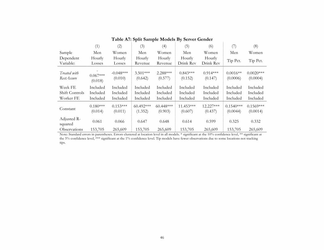
Table A7: Split Sample Models By Server Gender
(1) (2) (3) (4) (5) (6) (7) (8)
Sample Men Women Men Women Men Women Men Women Dependent Variable:
Hourly Losses
Hourly Losses
Hourly Revenue
Hourly Revenue
Hourly Drink Rev
Hourly Drink Rev Tip Pct. Tip Pct.
Treated with RestAssure
-0.067*** (0.018)
-0.048*** (0.010)
3.501*** (0.642)
2.288*** (0.577)
0.843*** (0.152)
0.914*** (0.147)
0.0016** (0.0006)
0.0020*** (0.0004)
Week FE Included Included Included Included Included Included Included Included Shift Controls Included Included Included Included Included Included Included Included Worker FE Included Included Included Included Included Included Included Included
Constant 0.180*** (0.014)
0.153*** (0.011)
60.492*** (1.352)
60.448*** (0.903)
11.453*** (0.607)
12.227*** (0.437)
0.1540*** (0.0044)
0.1569*** (0.0014)
Adjusted R-squared 0.061 0.066 0.647 0.648 0.614 0.599 0.325 0.332
Observations 153,705 265,609 153,705 265,609 153,705 265,609 153,705 265,609 Note: Standard errors in parentheses. Errors clustered at location level in all models. * significant at the 10% confidence level, ** significant at the 5% confidence level, *** significant at the 1% confidence level. Tip models have fewer observations due to some locations not tracking tips.
46