Sustainable water resource management

under hydrological uncertainty

Newsha K. Ajami,1 George M. Hornberger,2 and David L. Sunding3

Received 6 December 2007; revised 2 June 2008; accepted 12 August 2008; published 6 November 2008.

[1] A proper understanding of the sources and effects of uncertainty is needed to achievethe goals of reliability and sustainability in water resource management and planning.Many studies have focused on uncertainties relating to climate inputs (e.g., precipitationand temperature), as well as those related to supply and demand relationships. In theend-to-end projection of the hydrological impacts of climate variability, however,hydrological uncertainties have often been ignored or addressed indirectly. In this paper,we demonstrate the importance of hydrological uncertainties for reliable water resourcesmanagement. We assess the uncertainties associated with hydrological inputs, parameters,and model structural uncertainties using an integrated Bayesian uncertainty estimatorframework. Subsequently, these uncertainties are propagated through a simple reservoirmanagement model in order to evaluate how various operational rules impact thecharacteristics of the downstream uncertainties, such as the width of the uncertaintybounds. By considering different operational rules, we examine how hydrologicaluncertainties impact reliability, resilience, and vulnerability of the management system.The results of this study suggest that a combination of operational rules (i.e., an adaptiveoperational approach) is the most reliable and sustainable overall management strategy.

Citation: Ajami, N. K., G. M. Hornberger, and D. L. Sunding (2008), Sustainable water resource management under hydrological

uncertainty, Water Resour. Res., 44, W11406, doi:10.1029/2007WR006736.

1. Introduction

[2] During the past decade there has been a surge in thedevelopment of techniques for assessing various sources ofuncertainty associated with hydrological forecasts [e.g.,Beven and Binley, 1992; Kuczera and Parent, 1998; Vrugtet al., 2003; Maier and Ascough, 2006; Ajami et al., 2007].Despite this progress, links between estimated hydrologicaluncertainties and water resources management uncertaintieshave not been extensively explored. Investigation of suchlinkages is especially important since it is not clear howuncertainty in scenario projections might affect the formu-lation of robust operational rules for reservoir management.This can directly impact the outcome of water resourcesplanning and management studies, especially climatechange studies that use climate forecasts (such as precipi-tation and temperature) to force hydrological models andconsequently project the impact of climate change onmanaging water resources [e.g., Chao, 1999; Maurer andDuffy, 2005; Vicuna et al., 2007]. None of these studiesspecifically account for the uncertainties associated with thehydrological modeling step, including model parametersand model structural uncertainties. Reliable hydrologic

predictions with estimates of associated uncertainties canprovide decision makers with information that allows themto incorporate risk in decision making and therefore mitigatesome of the social, economical and environmental impact ofpoor and conservative operational rules.[3] Georgakakos et al. [1998] generated an ensemble of

inflow forecasts for a reservoir by using a Monte Carloapproach that generated plausible atmospheric-forcingensembles based on historical climate variability. Using thisapproach they estimated measures of hydrologic forecastuncertainty assuming they had generated enough climateensembles to capture all the possible streamflow inputs tothe reservoir. They found that uncertainty projection is veryimportant for effective decision making and water resourcesmanagement. However, they did not assess any othersources of uncertainty such as hydrologic model structuraland parameter uncertainty that would impact the inputs tothe reservoir. Later, Yao and Georgakakos [2001] assessedthe sensitivity of reservoir performance under varioushistorical and climate scenarios. They went a step furtherthan Georgakakos et al. [1998] and in addition to climate-driven ensembles (GCM-conditioned ESPs), they usedhistorical analog extended streamflow prediction (analogESP), hydrologic ESP (which uses physical representationof Folsom watershed), operational forecast and finallyperfect forecast to create streamflow ensembles which werepropagated through the Folsom reservoir. They found thatthe ensemble reliability and forecast spread are two impor-tant factors that need to be used in decision making foreffective reservoir management and better handling theassociated risk. Yao and Georgakakos [2001] did notquantify and assess various sources of uncertainties that

1Berkeley Water Center, University of California, Berkeley, California,USA.

2Institute for Energy and Environment, Vanderbilt University, Nashville,Tennessee, USA.

3Department of Agricultural and Resource Economics, University ofCalifornia, Berkeley, California, USA.

Copyright 2008 by the American Geophysical Union.0043-1397/08/2007WR006736$09.00

W11406

WATER RESOURCES RESEARCH, VOL. 44, W11406, doi:10.1029/2007WR006736, 2008ClickHere

for

FullArticle

1 of 10

impacts inflow to the reservoir, explicitly. They generated aset of ensembles of streamflow inputs to the reservoir andattempted to indirectly address some of the hydrologicaluncertainties such as input (by including GCM-conditionedESPs and hydrologic ESP), parameter and state uncertainty(by using a stochastic framework), however they did notaccount for hydrologic model structural uncertainty. Boththese studies [Georgakakos et al., 1998; Yao andGeorgakakos, 2001] attempted to address in different waysthe importance of assessing various sources of hydrologicaluncertainties for more efficient water resource management,however they did not use an integrated approach to quantifyoverall and end-to-end hydrological uncertainties that im-pact streamflow inputs to the reservoir. Another commonapproach to studying how hydrological variability affectswater supply reliability is to use a historical sequence ofmeasured hydrological variables [e.g., Brekke et al., 2004;Cai and Rosegrant, 2004]. This approach avoids the uncer-tainty introduced from using a hydrological model, but isseriously limited by use of a relatively short record and stillsuffers from an inherent measurement uncertainty. Further,given climate change and some other factors, history willnot repeat itself, and the use of historical information canlead to the development of inefficient and ineffective watermanagement strategies.[4] In this paper we study the characteristics of hydro-

logical uncertainties as they are propagated through a waterresource management system. A state-of-the-art Bayesianframework called integrated Bayesian uncertainty estimator(IBUNE) [Ajami et al., 2007], was used to quantify input,parameter and hydrological model structural uncertainties.Subsequently, the simulated streamflow ensembles are usedto force a hypothetical reservoir system to evaluate theimpacts of operational rules on the way hydrologicaluncertainties are propagated through a water resourcessystem. We show how the characteristics of uncertainty

change as the reservoir is operated on the basis of differentsets of operational rules.

2. Methods

2.1. Study Site

[5] For this study we used data for the watersheds thatcontribute to the Shasta reservoir in the upper portion of theSacramento River, California (Figure 1). This upper portionof the watershed was subdivided into twelve subcatchmentsthat contribute to Shasta, with a monthly climate time seriesderived from the 1/8� gridded daily time series computed asan average of all grid cell values within the individualcatchment [Maurer et al., 2002]. The Shasta reservoir servesmultiple purposes including flood control, irrigation, mu-nicipal and industrial water supplies, and hydropowergeneration [Environmental Protection Agency, 2005].[6] Monthly precipitation was calculated as the sum of

the daily values for the period 1962 through 1994. Demanddata and other climate variable, including temperature, windspeed and humidity were each specified as monthly valuesfor each catchment. The climatology of the Upper Sacra-mento River is dominated by winter snowfall and dry, warmsummers with little or no precipitation.

2.2. Integrated Assessment of HydrologicalUncertainty

[7] Hydrologic models are simple mathematical concep-tualizations of complex and spatially distributed watershedprocesses that can be used to provide estimates of currentand future hydrologic events. The reliability of these modelsdepends on proper parameter and state estimation; however,errors inherent in meteorological and hydrological observa-tions, model states, model parameters, and model structureultimately introduce bias and uncertainty into the applica-tion. When models are applied for hydrologic prediction tobe used as reservoir inputs, incomplete accounting of these

Figure 1. The 12 catchments of the Upper Sacramento that contribute to the upper Shasta reservoir(40.8068 latitude, �121.3808 longitude, 1483 m altitude).

2 of 10

W11406 AJAMI ET AL.: WATER RESOURCES AND HYDROLOGICAL UNCERTAINTY W11406

uncertainties may lead to unreliable and inefficient man-agement of our water resources.[8] Various hydrological models, regardless of their com-

plexity, suffer from parameter and model structural uncer-tainties, therefore under the same input forcing performdifferently and result in different streamflow predictions[Reed et al., 2004]. The problem of computing streamflowunder conditions of input, model structure, and parameteruncertainty can be formulated as

yk;t ¼ f It; qk ;Mk ; tð Þ; ð1Þ

where yk,t represents streamflow estimate under model K attime t, It is input (e.g., precipitation) at time t, qk, isparameters of the model K, Mk is the model under studyfrom the pool of models and t is time.[9] We use IBUNE [Ajami et al., 2007] to account for the

various sources of uncertainty. To account for model struc-tural uncertainty we study and combine three hydrologicmodels, the Sacramento Soil Moisture Accounting model(SAC-SMA, 13 parameters [Burnash et al., 1973]), theSimple Water Balance model (SWB, five parameters[Schaake et al., 1996]) and the Hydrological Model(HYMOD, five parameters [Boyle, 2001]). For each modelK (MK) we need to assess uncertainty associated with themodel parameter estimation pk(qjyobs, yk,t, Mk) consideringobserved streamflow data, yobs and consequently the prob-ability of correctness of the estimated streamflow using thatmodel, pk(yk,tjq, yobs, Mk). To account for input forcinguncertainty, we introduce an input error model in the formof multipliers, It = 8tIt

obs, 8t � N(m8, s8). We assume thatthe multipliers 8t at each time step are drawn from someidentical normal distributions with unknown mean (m8) andstandard deviation (s8). The unknown mean and standarddeviation are added to the list of hydrological modelparameters to be estimated using a probabilistic parameterestimation method such as shuffle complex evolution Me-tropolis (SCEM) [Vrugt et al., 2003].[10] The climatological data (1962–1994) were used as

the forcing data for the abovementioned three differenthydrological models. The models are run in simulationmode using all the available data. IBUNE first estimatesthe parameters of the three models and assesses the uncer-tainty associated with the model parameters and the inputforcing using SCEM [Vrugt et al., 2003]. Later IBUNEaccounts for model structural uncertainty in streamflowsimulation by combining, the estimated streamflow gener-ated by the individual hydrological models using theBayesian model averaging approach. Bayesian model aver-aging (BMA) [Hoeting et al., 1999] is a probabilisticmultimodel combination technique that combines models

on the assumption that at each particular time step, there isonly one best ensemble member or model but we do notknow which one. BMA assigns weights to each model.These weights represent the likelihood of each model beinga correct model and are defined on the basis of overallperformance of each model in representing observedstreamflow. The final product of this step of IBUNE is aset of streamflow ensembles that represent the most prob-able streamflow estimate at each time step with its associ-ated uncertainty from input (precipitation error), modelparameter estimation, and model structural deficiencies(more details on IBUNE are given by Ajami et al.[2007]). These streamflow ensembles then are used as aninput to our management model. The accuracy of theestimated uncertainty bounds using IBUNE are measuredby the percentage of observations falling within thesebounds while they stay as narrow as possible. If theestimated uncertainty bounds are narrow but do not captureobservation points they are not taken to be accurate becausethey underestimate the overall uncertainty in the system.Also if the estimated uncertainty bounds capture all theobservation points because they are too wide, their precisionis questionable because they overestimate the uncertainty inthe system. If none of the models that are being used capturea certain event there is a high chance that the combinationwill not capture that event either. Therefore missing some ofevents may be a result of underestimation of model struc-tural uncertainty in the system. This shortcoming could beaddressed by considering additional hydrologic models withdifferent capacities and complexity levels in the model pool.This type of adjustment is beyond the scope of this paperand will not be discussed further. For further discussion onthe matter, readers are encouraged to review the work byAjami et al. [2007].

2.3. Reservoir Operation and Management Scenarios

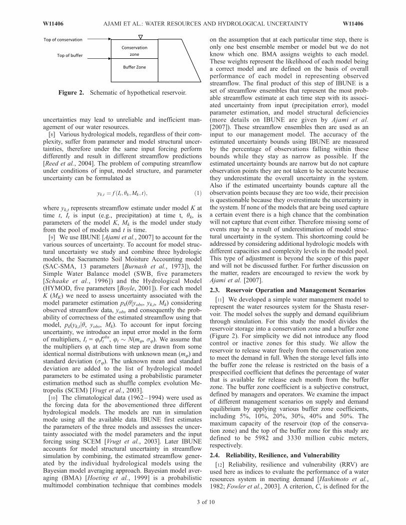
[11] We developed a simple water management model torepresent the water resources system for the Shasta reser-voir. The model solves the supply and demand equilibriumthrough simulation. For this study the model divides thereservoir storage into a conservation zone and a buffer zone(Figure 2). For simplicity we did not introduce any floodcontrol or inactive zones for this study. We allow thereservoir to release water freely from the conservation zoneto meet the demand in full. When the storage level falls intothe buffer zone the release is restricted on the basis of aprespecified coefficient that defines the percentage of waterthat is available for release each month from the bufferzone. The buffer zone coefficient is a subjective construct,defined by managers and operators. We examine the impactof different management scenarios on supply and demandequilibrium by applying various buffer zone coefficients,including 5%, 10%, 20%, 30%, 40% and 50%. Themaximum capacity of the reservoir (top of the conserva-tion zone) and the top of the buffer zone for this study aredefined to be 5982 and 3330 million cubic meters,respectively.

2.4. Reliability, Resilience, and Vulnerability

[12] Reliability, resilience and vulnerability (RRV) areused here as indices to evaluate the performance of a waterresources system in meeting demand [Hashimoto et al.,1982; Fowler et al., 2003]. A criterion, C, is defined for the

Figure 2. Schematic of hypothetical reservoir.

W11406 AJAMI ET AL.: WATER RESOURCES AND HYDROLOGICAL UNCERTAINTY

3 of 10

W11406

water supply sources where an unsatisfactory conditionoccurs when the specified demand is not met. Here, weexpect that the reservoir will supply 100% of the demanddownstream, therefore Ct is defined as the total demand thatneeds to be met at every time step. The time series ofmonthly demand coverage, Xt, are evaluated. Index Ztsignifies a satisfactory or unsatisfactory state of the system.On the basis of our definition of Ct, if all the demand is metthe system is in a satisfactory (S) state and Zt is one,otherwise in an unsatisfactory (U) state and Zt is zero[Hashimoto et al., 1982]:

Zt ¼1; if Xt 2 S

0; if Xt 2 U :

8<: ð2Þ

An index, Wt, is defined to capture the transitions betweensatisfactory and unsatisfactory states [Hashimoto et al.,1982]:

Wt ¼1; if Xt 2 U and Xtþ1 2 S

0; otherwise:

8<: ð3Þ

Hashimoto et al. [1982] treat reliability as a binary measureusing index Zt. In other words, the system either satisfies thepredefined criterion for meeting demand and is notpenalized, or does not satisfy the criterion and is penalized.Here is this study, we measure reliability on the basis ofwhether the system meets the prespecified demand criterionand if not, what percentage of the demand has been met (or

not been met) over the desired period (a year or the entiresimulation period):

Reliability CR ¼

XTi¼1

Xi

XTi¼1

Ci

: ð4Þ

Now, if the periods of unsatisfactory state Xt are J1, . . ., JNthen resilience and vulnerability are defined as follows[Hashimoto et al., 1982; Fowler et al., 2003], where T is thetotal length of the time series:

Resilience CRS ¼

XTt¼1

Wt

T �XTt¼1

Zt

ð5Þ

Vulnerability CV ¼ maxXt2Ji

C � Xt; i ¼ 1::::N

( ): ð6Þ

Here, reliability, CR, measures the percentage of the demandthat has been met and resilience, CRS, indicates the recoveryspeed of the system from the state of failure (unsatisfactory).Reliability and resilience are both positive measures (thehigher, the better). Vulnerability, CV, is a measure of theextent of failure which here has been shown as the maximumshortfall among all the continuous failure or unsatisfactory

Figure 3. Streamflow predictions and the 95% uncertainty bounds associated with input, modelparameters, and model structural uncertainty, assessed by IBUNE.

4 of 10

W11406 AJAMI ET AL.: WATER RESOURCES AND HYDROLOGICAL UNCERTAINTY W11406

periods. In other words, if there are n unsatisfactory periods,on the basis of equation (6), we first calculate the sum ofshortfall over each period and then select the highest of thesevalues as vulnerability. This value shows how poorly thesystem can perform during an unsatisfactory period inmeeting the demand. Vulnerability is a negative measure (thesmaller, the better). For more details on these measures, thereader is referred to Hashimoto et al. [1982] and Fowler etal. [2003].[13] An efficient management and operational strategy

should improve the reliability and resilience of the systemwhile reducing vulnerability. Reliability and vulnerabilityare inversely related. As reliability of the system increases,the vulnerability of the system lessens. However, thisrelationship is not direct and linear; trade-off decisions oftenneed to be made in an attempt to accommodate both factorsand to find an acceptable balance between reliability andvulnerability of the system.[14] To evaluate overall performance of the system under

various operational rules, we can calculate sustainabilitymeasure [Loucks, 1997] by combining reliability, resilienceand vulnerability indices as follows:

S ¼ Reliability Resilience 1� Relative Vulnerabilityð Þ; ð7Þ

where reliability and resilience are calculated earlier on thebasis of equations (4) and (5). Relative vulnerabilityrepresents dimensionless vulnerability measure and isdefined as follows:

Relative Vulnerability ¼ CVXt2Jn

Xt

; ð8Þ

where CV is calculated using equation (6), Jn refers to theunsatisfactory period that CV represents and Xt is demand attime step t. The multiplication in equation (7) gives addedweight to the statistical measure that has the lowest value,therefore does not overestimate the system’s performance.Sustainability is a positive measure as well, the higher thebetter. This index reflects the overall performance of thesystem considering the RRV measures.

3. Results

3.1. Change in Characteristics of the Uncertainty

[15] The IBUNE procedure resulted in a simulation oftime-variant probability distributions of streamflow(Figure 3). The IBUNE uncertainty bounds associated withinput, parameter and model structural uncertainty, are rea-

Figure 4. Reservoir storage capacity under various conditions. The gray shading represents thehydrological uncertainties which have been propagated through the reservoir: (a) 5% buffer zonecoefficient, (b) 20% buffer zone coefficient, (c) 50% buffer zone coefficient, and (d) adaptive scenario(5% and 20%).

W11406 AJAMI ET AL.: WATER RESOURCES AND HYDROLOGICAL UNCERTAINTY

5 of 10

W11406

sonably narrow while almost 95% of the observation pointsfall within the 95% forecast range (Figure 3). The uncer-tainty bounds fail to capture some of the peak values (Figure3). We are using monthly streamflow values so the peakflows do not represent flood events and missing them in theuncertainty bounds does not mean that the hydrologicmodels failed for our purposes.[16] The streamflow input realizations (5000 ensembles),

which were simulated on the basis of assessed hydrologicaluncertainties, are propagated through our simple reservoirsystem. The characteristics of these hydrological uncertain-ties change as they are propagated through the reservoir ateach time step on the basis of the operational rules(Figure 4). We observed that the uncertainty bounds forreservoir storage generally widen. Also we can see thatcompared to the streamflow input uncertainty bound distri-bution (Figure 5a), the distribution of the width of thereservoir storage uncertainty bounds is bimodal. The bi-modality in the distribution is the result of two facts: (1) thereservoir capacity limitations and (2) buffer zone coeffi-cient. The first mode in Figures 5b–5h is created when thestorage level hits its maximum capacity (top of the conser-vation zone). Regardless of streamflow input level, there isno more space available in the reservoir to store the water,therefore, all the streamflow ensembles result in a singlestorage level or storage levels with negligible differences.As we impose various operational rules the second center ofmass becomes more dominant in the probability distribution(Figure 5). These operational rules, as mentioned earlier,include the percentage of water in the buffer zone which isavailable to meet the demand downstream. Because thereservoir acts as an accumulator, the widening of theuncertainty bounds is inevitable during periods of decliningstorage. Therefore, even when there are no rules in place thewidth of the uncertainty bounds widens compared to

streamflow input (Figures 5a and 5b). Because reservoirhas capacity limitation, even under the no rules scenario(Figure 5b), we can see a very weak second mode in thedistribution of the width of reservoir storage capacityuncertainty bounds. Once the rules are put into place, theprobability distribution sustains its bimodal shape and thecenter of mass moves between 0.75 and 1 million cubicmeters (Figures 5c–5f). As the buffer coefficient (i.e., theavailable free water from the buffer zone) increases to meetthe demand, the distribution again takes its original shape(no rules in place, Figures 5g and 5h) and the uncertaintybounds widen some more. Once 30% of the water in thebuffer zone becomes available to meet the demand thedistribution of the uncertainty bounds begins to revert to avery weak bimodal distribution. By the time half of thewater in the buffer zone is available for release (C = 0.5),the uncertainty distribution essentially returns to that of the‘‘no operational rules’’ scenario (Figure 5).[17] Examination of the width of the propagated hydro-

logical uncertainty bounds for unmet demand shows behav-ior opposite to reservoir storage capacity (Table 1). As thewidth of the uncertainty bounds enlarges with increase inreleased water, the width of the uncertainty bounds forunmet demand becomes narrower. This is expected sincemore water becomes available to meet the demand. Thewidth of the uncertainty bounds for unmet demand drops bymore than 50% as the buffer coefficient increases from 5%to 20%. Increases in the buffer coefficient beyond 20% donot significantly change the uncertainty bounds for unmetdemand (Table 1). This is expected since most of thedemand is met during normal years by taking 20% of thewater from the buffer zone and there is no need foradditional water. However during dry years by increasingthe buffer zone coefficient to more than 20%, regardless ofwhether more water becomes available to meet demand,

Figure 5. Distribution of the width of the reservoir storage uncertainty bounds under differentoperational rules.

6 of 10

W11406 AJAMI ET AL.: WATER RESOURCES AND HYDROLOGICAL UNCERTAINTY W11406

considerable deficiency continues to exist in storage andconsequently, cannot alleviate unmet demand. Therefore, nosignificant improvement (tightening) is seen in the width ofthe uncertainty bounds for the unmet demand as we increasethe buffer zone coefficient (Table 1).

3.2. Impacts of Operational Rules on SystemReliability, Resilience, and Vulnerability

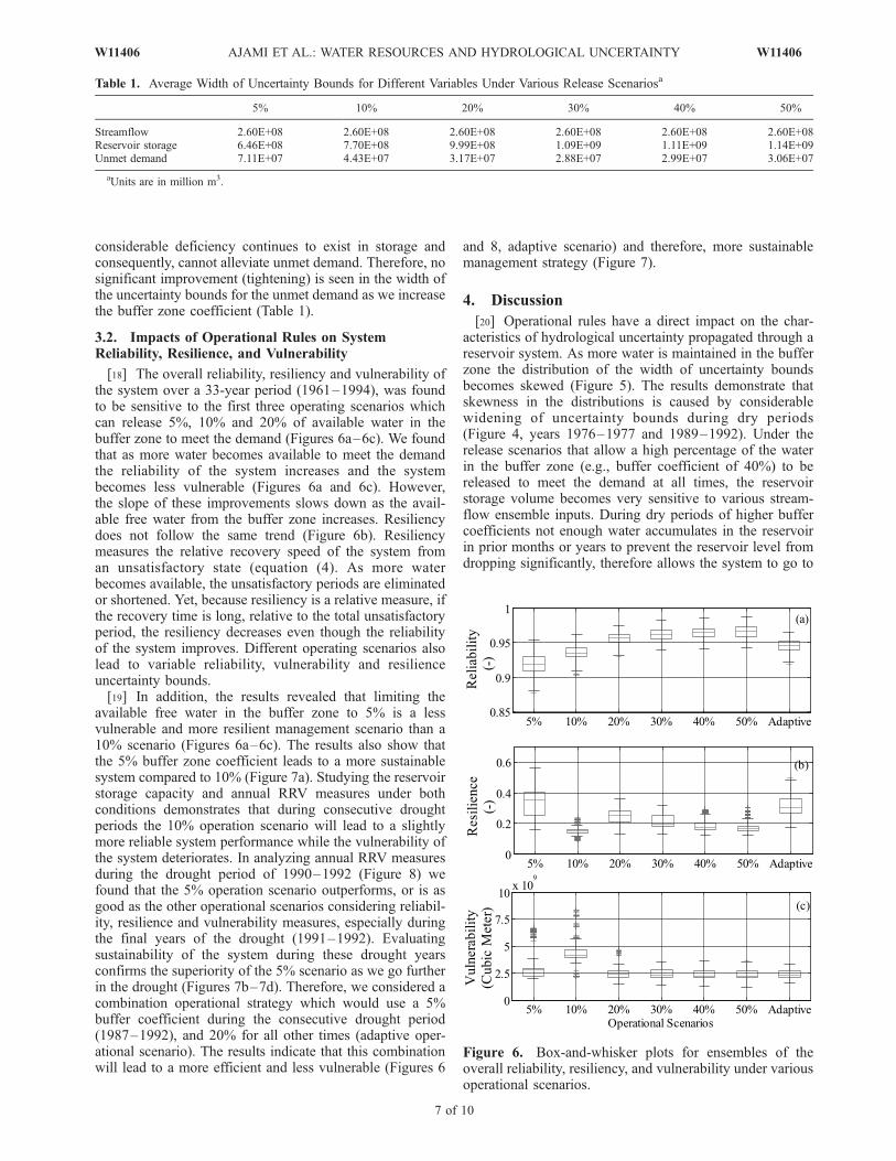
[18] The overall reliability, resiliency and vulnerability ofthe system over a 33-year period (1961–1994), was foundto be sensitive to the first three operating scenarios whichcan release 5%, 10% and 20% of available water in thebuffer zone to meet the demand (Figures 6a–6c). We foundthat as more water becomes available to meet the demandthe reliability of the system increases and the systembecomes less vulnerable (Figures 6a and 6c). However,the slope of these improvements slows down as the avail-able free water from the buffer zone increases. Resiliencydoes not follow the same trend (Figure 6b). Resiliencymeasures the relative recovery speed of the system froman unsatisfactory state (equation (4). As more waterbecomes available, the unsatisfactory periods are eliminatedor shortened. Yet, because resiliency is a relative measure, ifthe recovery time is long, relative to the total unsatisfactoryperiod, the resiliency decreases even though the reliabilityof the system improves. Different operating scenarios alsolead to variable reliability, vulnerability and resilienceuncertainty bounds.[19] In addition, the results revealed that limiting the

available free water in the buffer zone to 5% is a lessvulnerable and more resilient management scenario than a10% scenario (Figures 6a–6c). The results also show thatthe 5% buffer zone coefficient leads to a more sustainablesystem compared to 10% (Figure 7a). Studying the reservoirstorage capacity and annual RRV measures under bothconditions demonstrates that during consecutive droughtperiods the 10% operation scenario will lead to a slightlymore reliable system performance while the vulnerability ofthe system deteriorates. In analyzing annual RRV measuresduring the drought period of 1990–1992 (Figure 8) wefound that the 5% operation scenario outperforms, or is asgood as the other operational scenarios considering reliabil-ity, resilience and vulnerability measures, especially duringthe final years of the drought (1991–1992). Evaluatingsustainability of the system during these drought yearsconfirms the superiority of the 5% scenario as we go furtherin the drought (Figures 7b–7d). Therefore, we considered acombination operational strategy which would use a 5%buffer coefficient during the consecutive drought period(1987–1992), and 20% for all other times (adaptive oper-ational scenario). The results indicate that this combinationwill lead to a more efficient and less vulnerable (Figures 6

and 8, adaptive scenario) and therefore, more sustainablemanagement strategy (Figure 7).

4. Discussion

[20] Operational rules have a direct impact on the char-acteristics of hydrological uncertainty propagated through areservoir system. As more water is maintained in the bufferzone the distribution of the width of uncertainty boundsbecomes skewed (Figure 5). The results demonstrate thatskewness in the distributions is caused by considerablewidening of uncertainty bounds during dry periods(Figure 4, years 1976–1977 and 1989–1992). Under therelease scenarios that allow a high percentage of the waterin the buffer zone (e.g., buffer coefficient of 40%) to bereleased to meet the demand at all times, the reservoirstorage volume becomes very sensitive to various stream-flow ensemble inputs. During dry periods of higher buffercoefficients not enough water accumulates in the reservoirin prior months or years to prevent the reservoir level fromdropping significantly, therefore allows the system to go to

Table 1. Average Width of Uncertainty Bounds for Different Variables Under Various Release Scenariosa

5% 10% 20% 30% 40% 50%

Streamflow 2.60E+08 2.60E+08 2.60E+08 2.60E+08 2.60E+08 2.60E+08Reservoir storage 6.46E+08 7.70E+08 9.99E+08 1.09E+09 1.11E+09 1.14E+09Unmet demand 7.11E+07 4.43E+07 3.17E+07 2.88E+07 2.99E+07 3.06E+07

aUnits are in million m3.

Figure 6. Box-and-whisker plots for ensembles of theoverall reliability, resiliency, and vulnerability under variousoperational scenarios.

W11406 AJAMI ET AL.: WATER RESOURCES AND HYDROLOGICAL UNCERTAINTY

7 of 10

W11406

an unsatisfactory state in meeting the demand. This can leadto a very wide range of reservoir response depending on thedemand. The considerable drop in reservoir storage forlower inflow values from the simulation ensembles, thathappen under such scenarios, can cause some criticalproblems (such as failing to meet the agricultural and urbanwater demands or shortages in hydro electricity generation),especially during consecutive dry periods or drought spellswhen the reservoir does not have enough time to recoverfrom one crisis before the next one arrives.[21] We found that the distribution of the width of the

uncertainty bounds for operational scenarios of 5–30%buffer coefficient is less skewed compared to scenarios withlarger buffer coefficient (40% and 50%). When the reservoir

is full (or close to full), the uncertainty bounds are zero (orvery insignificant and narrow), creating one center of massaround zero bound width for all scenarios (Figure 5). Thesecond center of the mass around higher values in thebimodal distribution is created by even and uniform wid-ening of the uncertainty bounds throughout the simulationperiod around the buffer zone boundary line (Figures 4 and5). This widening mainly happens around the thresholdseparating the buffer zone from the conservation zoneespecially for the lower buffer zone coefficients. Reservoirstorage at the end of each month depends on the waterreleased to meet the demand, which is a function ofdemand, inflow to the reservoir during that month, andthe initial storage. For example, when stricter operational

Figure 7. Box-and-whisker plots for ensembles of sustainability measure.

Figure 8. Box-and-whisker plots for ensembles of annual reliability, resilience, and vulnerability undervarious operational scenarios for drought period of 1990–1992.

8 of 10

W11406 AJAMI ET AL.: WATER RESOURCES AND HYDROLOGICAL UNCERTAINTY W11406

rules are in place and the buffer zone coefficient is 5% andthe level of the reservoir is very close to the threshold, anysmall change in the inflow or outflow to the reservoir cancause the storage level to fluctuate between the two zonesfrom one time step to the other. In other words, thecombination of the inflow ensembles and the releaseensembles can lead to some chaotic reaction around thethreshold by jumping from one state to the other at differenttime steps (Figure 4). Since there is limited water availablein the buffer zone to be released under the stringentoperational rules (5% buffer zone coefficient), the widthof the uncertainty bounds becomes very narrow and uniformaround the threshold value during the simulation period,which leads to the denser second center of mass in thebimodal distribution (Figures 4 and 5). In contrast, looseroperational scenarios have a significant impact on theuncertainty bounds during dry periods since they allowreservoir storage to drop much lower in the buffer zone(Figure 4). This leads to significant widening of the uncer-tainty bounds and thus, skewness in the final distribution(Figure 5). To put this in perspective, we examined thedistribution of the width of the demand uncertainty boundsfor the 50% buffer zone coefficient, and found that thewidening and therefore skewness that is observed in reser-voir storage uncertainty bounds leads to the skewed distri-bution on the demand side as well. The widening of thedemand uncertainty bounds for higher buffer coefficients(30–50%) mainly happens toward the end of 1976–1977and 1989–1992 drought periods. As the reservoir tries tomeet the entire demand during the early years of drought byreleasing more water from the buffer zone, the storage levelgoes significantly down; consequently, there is not enoughwater in the later years of drought to meet the demand,especially for the ensembles with lower values. It is importantto keep in mind that we would like to have narrow and preciseuncertainty bounds that capture most of the observed valuesat all times. This may lead to more efficient and sustainableplanning and decrease risk. When the uncertainty boundsbecome too wide each given time step has many possibleevents that can take place which can significantly differ fromeach other. Such wide spread possibilities can increase risk offailure in decisionmaking because it is hard to come upwith aset of rules that can handle all possible events. Decisionmakers can try to manage such cases by using a set of veryconservative operational rules that would not fail under mostpossibilities. Such conservative decision rules can have veryinefficient social and economical impacts. Therefore, accu-racy and reliability in the hydrological forecast can mitigatesuch impacts and help decision makers to better handle therisk in decision making.[22] The overall reliability and vulnerability measures

showed considerable sensitivity to the 5% to 20% opera-tional rules. However, as the buffer coefficient is increased(30% to 50%), this sensitivity faded away and not muchimprovement was observed (neither in the mean value norin the width of the uncertainty bound) in increasing theavailable water. As the percentage of available water fromthe buffer zone is increased from 5% to 10%, both resilienceand vulnerability deteriorates while reliability improves.This is contrary to our expectation that the availability ofmore water from the buffer zone would improve the systemperformance on the basis of RRV measures, since there is

more water available to meet the demand (Figure 6). Wefound that this deterioration in the overall system perfor-mance can be attributed to the poor performance of the 10%operational scenario considering the resilience and vulner-ability, during consecutive drought years (Figure 8). The 5%operational scenario conserves some water by not fullymeeting the demand downstream, which helps increasesupply during the long drought periods, therefore beingable to meet the whole demand after a few months ofconservation. Therefore, the 5% operational scenarioimproves the resilience of the system by shortening theunsatisfactory periods (breaks them into two or three shortercycles rather than a one long one). This also leads to areduction in vulnerability compared to the 10% operationalscenario. The 5% scenario also performs as well as the otheroperational scenarios (30–50%) that provide more water tomeet the demand during dry periods (Figure 8).[23] Studying the uncertainty associated with each one of

these measures, one can see that the width of the uncertaintybounds on reliability and vulnerability does not changemuch from one operational rule to the other, especially aswe pass the 20% buffer coefficient. It seems that theuncertainty bounds on resilience are the most sensitive tothe operational rules. As the amount of available water fromthe buffer zone increases, resilience deteriorates while theuncertainty bounds narrow down (Figure 6c, comparing 5%to 50% buffer coefficient). To put these into perspective wetested the sustainability measure (Figure 7a). Close inves-tigation of an overall sustainability measure (Figure 7a)depicts that considering 5%, 40% and 50% buffer coeffi-cient almost leads to the same level of sustainability in thesystem considering their mean and the width of uncertaintybounds. Ten percent and 20 percent operational rules are theleast and the most sustainable scenarios, respectively. Theyalso lead to the narrowest (10%) and widest (20%) uncer-tainty bounds as well. Even though the mean value of thesustainability measure for the 20% operational rule has thehighest value, the uncertainty bounds around it are quitewide compared to all other scenarios, not a desirable factorfor decision makers because it can lead to development ofmore conservative and less efficient management rules todeal with the risk.[24] We found that a trade-off decision needs to be made

on the basis of the overall and annual reliability, resilienceand vulnerability of the system. The results demonstrate thatefficient and sustainable management is achievable throughthe use of a combination of buffer coefficients (Figures 7)that would lead to high overall reliability while maintaininghigh resilience and low vulnerability (Figures 6 and 8).Under the existing state of demand, our results indicate thatthe combination of a 20% release from the buffer zoneduring the normal and wet years and a 5% release duringconsecutive dry years, is the most efficient managementapproach here, considering the RRV measures (Figures 6and 8) and sustainability index (Figure 7).[25] The combination scenario (adaptive) also leads to the

narrowest uncertainty bounds in the reservoir storage sim-ulations during the critical years of 1989–1992 (Figure 4)and the overall sustainability measure (Figure 7a), which isvery important because it makes decision making andplanning easier and less uncertain. As demonstrated in thepioneering study of Burness and Quirk [1979], and in later

W11406 AJAMI ET AL.: WATER RESOURCES AND HYDROLOGICAL UNCERTAINTY

9 of 10

W11406

work by Sunding et al. [2008], there can be a largeeconomic value associated with reductions in uncertaintyabout future water supplies. The productivity of water isdetermined in large part by capital investments that increasethe value of water used in production processes. Uncertaintyis a disincentive to making such investments; consequently,resolution of uncertainty can improve the efficiency andproductivity of water use and help to cope with conditionsof scarcity and increasing competition. Also, accuratelyaccounting for various sources of uncertainty can reducethe social and economical impacts of inefficient and unsus-tainable decision making that is caused by poor knowledgeof inherited uncertainty and therefore, inaccuracy of thehydrological forecast.

5. Summary

[26] This paper evaluates the importance of hydrologicaluncertainty in sustainable and efficient management ofwater resource systems. The hydrological uncertainties wereestimated using the recently developed uncertainty estima-tion framework integrated Bayesian uncertainty estimator(IBUNE) [Ajami et al., 2007]. These uncertainties were laterpropagated through a reservoir system and various opera-tional rules were put into place to examine the impact ofthese rules on the characteristics of hydrological uncertain-ties. The change in the distribution of the width of uncer-tainty bounds from streamflow to reservoir storage capacityleads to nonintuitive effects in terms of measures of systemperformance. On the basis of the presented results, we inferthat an adaptive operational approach where the decisionmaker adjusts the operational rules on the basis of inflowclimate forecast and the existing state of reservoir storage ateach given time step, can lead to a more efficient andsustainable management of the reservoir. Therefore, im-proved reservoir management solely depends on accuracyof the climate forecast ensembles that would lead to moreaccurate hydrological forecasts and effective use of theseensembles. Hence, accurately accounting for various sour-ces of uncertainty that influence our forecasted inflow to thereservoir provides better and more precise information todecision makers and will help them operate a water resourcesystem in a more sustainable, socially and economicallyefficient way.

[27] Acknowledgments. This work was supported by the UC Berke-ley Water Center. The valuable comments by Richard Vogel and ananonymous reviewer significantly improved this paper and are gratefullyacknowledged.

ReferencesAjami, N. K., Q. Duan, and S. Sorooshian (2007), An integrated hydrologicBayesian multimodel combination framework: Confronting input, para-meter, and model structural uncertainty in hydrologic prediction, WaterResour. Res., 43, W01403, doi:10.1029/2005WR004745.

Beven, K., and A. Binley (1992), The future of distributed models: Modelcalibration and uncertainty prediction, Hydrol. Processes, 6, 279–298,doi:10.1002/hyp.3360060305.

Boyle, D. (2001), Multicriteria calibration of hydrological models, Ph.D.dissertation, Univ. of Ariz., Tucson.

Brekke, L., N. L. Miller, K. E. Bashford, N. W. T. Quinn, and J. A. Dracup(2004), Climate change impacts uncertainty for water resources in theSan Joaquin River Basin, California, J. Am. Water Resour. Assoc., 40,149–164, doi:10.1111/j.1752-1688.2004.tb01016.x.

Burnash, R. J., R. L. Ferral, and R. A. McGuire (1973), A generalizedstreamflow simulation system conceptual modeling for digital computers,

technical report, Natl. Weather Serv., U.S. Dep. of Commer., SilverSpring, Md.

Burness, H. S., and J. P. Quirk (1979), Appropriative water rights and theefficient allocation of resources, Am. Econ. Rev., 69(1), 25–37.

Cai, X., and M. W. Rosegrant (2004), Irrigation technology choices underhydrologic uncertainty: A case study from Maipo River Basin, Chile,Water Resour. Res., 40, W04103, doi:10.1029/2003WR002810.

Chao, P. (1999), Great Lakes water resources: Climate change impact ana-lysis with transient GCM scenarios, J. Am. Water Resour. Assoc., 35,1485–1499, doi:10.1111/j.1752-1688.1999.tb04232.x.

Environmental Protection Agency (2005), Shasta Lake water resources in-vestigation, Shasta and Tehama counties, CA, Fed. Regist. Environ. Doc.70 (194) 58744-58746, Washington, D. C. (Available at http://www.epa.gov/fedrgstr/EPA-IMPACT/2005/October/Day-07/i20169.htm)

Georgakakos, A. P., H. Yao, M. Mullusky, and K. P. Georgakakos (1998),Impacts of climate variability on the operational forecast and manage-ment of the Upper Des Moines River basin, Water Resour. Res., 34(4),799–821.

Fowler, H. J., C. G. Kilsby, and P. E. O’Connell (2003), Modeling theimpacts of climatic change and variability on the reliability, resilience,and vulnerability of a water resource system, Water Resour. Res., 39(8),1222, doi:10.1029/2002WR001778.

Hashimoto, T., J. R. Stedinger, and D. P. Loucks (1982), Reliability, resi-liency and vulnerability criteria for water resource system performanceevaluation, Water Resour. Res. , 18(1), 14 – 20, doi:10.1029/WR018i001p00014.

Hoeting, J. A., D. Madigan, A. E. Raftery, and C. T. Volinsky (1999),Bayesian model averaging: A tutorial, Stat. Sci., 14(4), 382 –417,doi:10.1214/ss/1009212519.

Kuczera, G., and E. Parent (1998), Monte Carlo assessment of parameteruncertainty in conceptual catchment models: The metropolis algorithm,J. Hydrol., 211, 69–85, doi:10.1016/S0022-1694(98)00198-X.

Loucks, D. P. (1997), Quantifying trends in system sustainability, Hydrol.Sci. J., 42(4), 513–530.

Maier, H. R., and J. C. Ascough II (2006), Uncertainty in environmentaldecision-making: Issues, challenges and future directions, in Proceedingsof the iEMSs Third Biennial Meeting: Summit on Environmental Model-ling and Software [CD-ROM], edited by A. Voinov, A. Jakeman, andA. Rizzoli, Int. Environ. Modell. and Software Soc., Burlington, Vt.(Available at http://www.iemss.org/iemss2006/sessions/all.html)

Maurer, E. P., and P. B. Duffy (2005), Uncertainty in projections of stream-flow changes due to climate change in California, Geophys. Res. Lett.,32, L03704, doi:10.1029/2004GL021462.

Maurer, E. P., A. W. Wood, J. C. Adam, D. P. Lettenmaier, and B. Nijssen(2002), A long term hydrologically-based data set of land surface fluxesand states for the conterminous United States, J. Clim., 15, 3237–3251,doi:10.1175/1520-0442(2002)015<3237:ALTHBD>2.0.CO;2.

Reed, S., V. Koren, M. Smith, Z. Zhang, F. Moreda, D. J. Seo, and D. M. I.P. Participants (2004), Overall distributed model intercomparison projectresults, J. Hydrol., 298, 27–60, doi:10.1016/j.jhydrol.2004.03.031.

Schaake, J. C., V. I. Koren, Q. Y. Duan, K. Mitchell, and F. Chen (1996),Simple water balance model for estimating runoff at different spatial andtemporal scales, J. Geophys. Res., 101(D3), 7461–7475, doi:10.1029/95JD02892.

Sunding, D., G. Moreno, D. Osgood, and D. Zilberman (2008), The valueof investments in water supply reslibility, Am. J. Agric. Econ., in press.

Vicuna, S., E. P. Maurer, P. Edwin, B. Joyce, J. A. Dracup, and D. Purkey(2007), The sensitivity of California water resources to climate changescenarios, J. Am. Water Resour. Assoc., 43, 482 –498, doi:10.1111/j.1752-1688.2007.00038.x.

Vrugt, J. A., H. V. Gupta, W. Bouten, and S. Sorooshian (2003), A ShuffledComplex Evolution Metropolis algorithm for optimization and uncer-tainty assessment of hydrologic model parameters, Water Resour. Res.,39(8), 1201, doi:10.1029/2002WR001642.

Yao, H., and A. Georgakakos (2001), Assessment of Folsom Lake responseto historical and potential future climate scenarios 2. Reservoir manage-ment, J. Hydrol., 249, 176–196, doi:10.1016/S0022-1694(01)00418-8.

����������������������������N. K. Ajami, Berkeley Water Center, University of California, Berkeley,

CA 94720-1766, USA. (newshaajami@berkeley.edu)

G. M. Hornberger, Institute for Energy and Environment, VanderbiltUniversity, Nashville, TN 37240, USA.

D. L. Sunding, Department of Agricultural and Resource Economics,University of California, Berkeley, CA 94720-3310, USA.

10 of 10

W11406 AJAMI ET AL.: WATER RESOURCES AND HYDROLOGICAL UNCERTAINTY W11406