climate change and global water resources: sres emissions and

Global Environmental Change 14 (2004) 31–52

ARTICLE IN PRESS

0959-3780/$ - see

doi:10.1016/j.glo

Climate change and global water resources: SRES emissions andsocio-economic scenarios

Nigel W. Arnell

School of Geography, University of Southampton, Southampton SO17 1BJ, UK

Abstract

In 1995, nearly 1400 million people lived in water-stressed watersheds (runoff less than 1000m3/capita/year), mostly in south west

Asia, the Middle East and around the Mediterranean. This paper describes an assessment of the relative effect of climate change and

population growth on future global and regional water resources stresses, using SRES socio-economic scenarios and climate

projections made using six climate models driven by SRES emissions scenarios. River runoff was simulated at a spatial resolution of

0.5� 0.5� under current and future climates using a macro-scale hydrological model, and aggregated to the watershed scale to

estimate current and future water resource availability for 1300 watersheds and small islands under the SRES population

projections. The A2 storyline has the largest population, followed by B2, then A1 and B1 (which have the same population). In the

absence of climate change, the future population in water-stressed watersheds depends on population scenario and by 2025 ranges

from 2.9 to 3.3 billion people (36–40% of the world’s population). By 2055 5.6 billion people would live in water-stressed watersheds

under the A2 population future, and ‘‘only’’ 3.4 billion under A1/B1.

Climate change increases water resources stresses in some parts of the world where runoff decreases, including around the

Mediterranean, in parts of Europe, central and southern America, and southern Africa. In other water-stressed parts of the world—

particularly in southern and eastern Asia—climate change increases runoff, but this may not be very beneficial in practice because

the increases tend to come during the wet season and the extra water may not be available during the dry season. The broad

geographic pattern of change is consistent between the six climate models, although there are differences of magnitude and direction

of change in southern Asia.

By the 2020s there is little clear difference in the magnitude of impact between population or emissions scenarios, but a large

difference between different climate models: between 374 and 1661 million people are projected to experience an increase in water

stress. By the 2050s there is still little difference between the emissions scenarios, but the different population assumptions have a

clear effect. Under the A2 population between 1092 and 2761 million people have an increase in stress; under the B2 population the

range is 670–1538 million, respectively. The range in estimates is due to the slightly different patterns of change projected by the

different climate models. Sensitivity analysis showed that a 10% variation in the population totals under a storyline could lead to

variations in the numbers of people with an increase or decrease in stress of between 15% and 20%. The impact of these changes on

actual water stresses will depend on how water resources are managed in the future.

r 2003 Elsevier Ltd. All rights reserved.

Keywords: Climate change impacts; Global water resources; Water resources stresses; SRES emissions scenarios; Macro-scale hydrological model;

Multi-decadal variability

1. Introduction

The UN Comprehensive Assessment of the Fresh-water Resources of the World (WMO, 1997) estimatedin 1997 that approximately a third of the world’spopulation was living in countries deemed to besuffering from water stress: they were withdrawing morethan 20% of their available water resources. Theassessment went on to estimate that up to two-thirdsof the world’s population would be living in water-stressed countries by 2025. Climate change due to an

front matter r 2003 Elsevier Ltd. All rights reserved.

envcha.2003.10.006

increasing concentration of greenhouse gases is likely toaffect the volume and timing of river flows andgroundwater recharge, and thus affect the numbersand distribution of people affected by water scarcity.Estimates of the effect of climate change, however,depend not only on the assumed emissions scenario andclimate model used to translate emissions into regionalclimates, but also on the assumed rate of populationchange.Since the UN Comprehensive Assessment of the

Freshwater Resources of the World was published in

ARTICLE IN PRESSN.W. Arnell / Global Environmental Change 14 (2004) 31–5232

1997, based on rather coarse national-scale data, therehave been a number of other global-scale assessments.Seckler et al. (1998, 1999) have assessed future waterresource scarcity at the global scale by 2025. Theyassumed no climate change, and their study concen-trated on the development of scenarios for water use,focusing particularly on irrigation use. Alcamo et al.(2000, 2003) refined their earlier assessment (Alcamoet al., 1997) by calculating water resources and resourcedemands at the river basin scale and using differentprojections of future demand: they did not, however,consider the effects of climate change. Their model wasalso used in UNEP’s Global Environment Outlook-3(UNEP, 2001), with different projections of futureresource use and including the effects of climate change(although the particular climate models used were notspecified). The Pilot Analysis of Global Ecosystems(PAGES) freshwater systems assessment (Revenga et al.,2000; World Resources Institute, 2000) also worked atthe major river basin scale, but used a different index ofwater resources stress: this study too did not consider theeffects of climate change, and like Alcamo et al. (1997)and UNEP (2001) projected substantial increases in thenumbers of people living in water-stressed basins, dueentirely to population growth. V .or .osmarty et al. (2000)compared demand growth and climate change scenariosat the 0.5� 0.5� scale, showing that over the next 25 yearsclimate change would have less effect on change in waterresources stresses than population and water demandgrowth. However, they did not explicitly compare thefuture situation with and without climate change.The aim of this paper is to present results of an

assessment of the implications of climate change for theglobal and regional numbers of people living in water-stressed watersheds, using consistent climate and socio-economic scenarios: the climatic effects of the differentIPCC SRES (IPCC, 2000) emissions scenarios arecompared with the assumed populations which gener-ated those emissions. The paper compares the relativeeffect of emissions scenario and population growth rateon the effects of climate change. It uses a macro-scalehydrological model to translate climate change scenariosconstructed from climate model simulations (using sixclimate models run with SRES emissions scenarios) intorunoff at the 0.5� 0.5� scale, and calculates waterresources stress indicators at the watershed scale. Acompanion paper (Arnell, 2003) describes the hydro-logical changes in more detail.

2. Methodology

The study adopted the conventional approach toclimate change impact assessment, following a change inclimate through to change in runoff, and then calculat-ing the implications for the number of people at risk of

increased water resources pressures. The primaryinnovation of the study lies in the use of a consistentset of emissions and socio-economic scenarios.The stages in the study were:

(i)
Construct scenarios for change in climate fromclimate model simulations of the climatic effects ofthe SRES emissions scenarios. Scenarios were con-structed from six climate models run with the SRESemissions scenarios—HadCM3, ECHAM4-OPYC,CSIRO-Mk2, CGCM2, GFDL r30 and CCSR/NIES2—characterising change in 30-year mean cli-mate relative to 1961–1990 by the 2020s (2010–2039),2050s (2040–2069) and 2080s (2070–2099).
(ii)
Apply these scenarios to a gridded baselineclimatology, describing climate over the period1961–1990 at a spatial resolution of 0.5� 0.5�
(New et al., 1999).
(iii) Run a macro-scale hydrological model at the
0.5� 0.5� resolution with the current and changedclimates to simulate 30 year time series of monthlyrunoff. Calculate average annual runoff from thesetime series.

(iv)
Sum the simulated runoff over approximately 1300watersheds and small islands to estimate water-shed-scale runoff volumes.
(v)
Determine the watershed population total undereach population growth scenario.
(vi)
Construct indicators of water resources stress foreach watershed from the simulated runoff andestimated watershed population.
These stages are described in more detail in the nextsection.

3. Emissions, climate, hydrological and socio-economic

scenarios

3.1. SRES population and emissions scenarios

The IPCCs Special Report on Emissions Scenarios(SRES) was published in 2000 (IPCC, 2000), andcontains a set of new projections of future greenhousegas emissions: these projections supersede the IS92family of projections. The starting point for eachprojection was a ‘‘storyline’’, describing the way worldpopulation, economies, political structure and lifestylesmay evolve over the next few decades. The storylineswere grouped into four scenario families, and ledultimately to the construction of six SRES markerscenarios (one of the families has three markerscenarios, the others one each). The four families canbe briefly characterised as follows:A1: Very rapid economic growth with increasing

globalisation, an increase in general wealth, with

ARTICLE IN PRESS

Table 1

Global population under the four SRES scenario families

A1 B1 A2 B2

Population (millions)

2025 7926 7926 8714 8036

2050 8709 8709 11778 9541

2085 7914 7914 14220 10235

N.W. Arnell / Global Environmental Change 14 (2004) 31–52 33

convergence between regions and reduced differences inregional per capita income. Materialist–consumeristvalues predominant, with rapid technological change.Three variants within this family make differentassumptions about sources of energy for this rapidgrowth: fossil intensive (A1FI), non-fossil fuels (A1T) ora balance across all sources (A1B).B1: Same population growth as A1, but development

takes a much more environmentally sustainable path-way with global-scale cooperation and regulation. Cleanand efficient technologies are introduced. The emphasisis on global solutions to achieving economic, social andenvironmental sustainability.A2: Heterogeneous, market-led world, with less rapid

economic growth than A1, but more rapid populationgrowth due to less convergence of fertility rates. Theunderlying theme is self-reliance and preservation oflocal identities. Economic growth is regionally oriented,and hence both income growth and technologicalchange are regionally diverse.B2: Population increases at a lower rate than A2 but

at a higher rate than A1 and B1, with development

Carbon emissions:IPCC SRES scenarios

0

5

10

15

20

25

30

1990 2000 2010 2020 2030 2040 2050 2060 2070 2080 2090 2100

Gt

Car

bon

per

year

A1B A1T A1F1 A2 B1 B2

Temperature change:IPCC SRES scenarios

0

1

2

3

4

5

1990 2000 2010 2020 2030 2040 2050 2060 2070 2080 2090 2100

o C r

elat

ive

to 1

990

A1B A1T A1FI A2 B1 B2

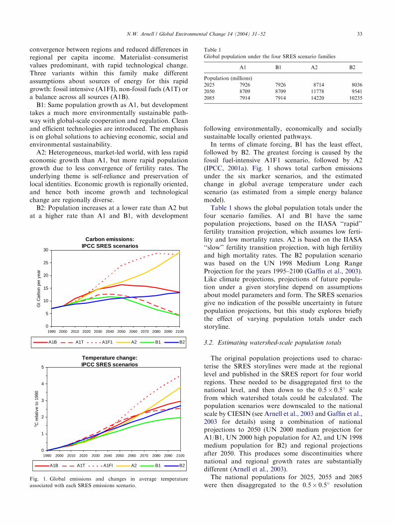
Fig. 1. Global emissions and changes in average temperature

associated with each SRES emissions scenario.

following environmentally, economically and sociallysustainable locally oriented pathways.In terms of climate forcing, B1 has the least effect,

followed by B2. The greatest forcing is caused by thefossil fuel-intensive A1F1 scenario, followed by A2(IPCC, 2001a). Fig. 1 shows total carbon emissionsunder the six marker scenarios, and the estimatedchange in global average temperature under eachscenario (as estimated from a simple energy balancemodel).Table 1 shows the global population totals under the

four scenario families. A1 and B1 have the samepopulation projections, based on the IIASA ‘‘rapid’’fertility transition projection, which assumes low ferti-lity and low mortality rates. A2 is based on the IIASA‘‘slow’’ fertility transition projection, with high fertilityand high mortality rates. The B2 population scenariowas based on the UN 1998 Medium Long RangeProjection for the years 1995–2100 (Gaffin et al., 2003).Like climate projections, projections of future popula-tion under a given storyline depend on assumptionsabout model parameters and form. The SRES scenariosgive no indication of the possible uncertainty in futurepopulation projections, but this study explores brieflythe effect of varying population totals under eachstoryline.

3.2. Estimating watershed-scale population totals

The original population projections used to charac-terise the SRES storylines were made at the regionallevel and published in the SRES report for four worldregions. These needed to be disaggregated first to thenational level, and then down to the 0.5� 0.5� scalefrom which watershed totals could be calculated. Thepopulation scenarios were downscaled to the nationalscale by CIESIN (see Arnell et al., 2003 and Gaffin et al.,2003 for details) using a combination of nationalprojections to 2050 (UN 2000 medium projection forA1/B1, UN 2000 high population for A2, and UN 1998medium population for B2) and regional projectionsafter 2050. This produces some discontinuities wherenational and regional growth rates are substantiallydifferent (Arnell et al., 2003).The national populations for 2025, 2055 and 2085

were then disaggregated to the 0.5� 0.5� resolution


using the Gridded Population of the World (GPW)Version 2 data set (CIESIN, 2000), which has a spatialresolution of 2.5� 2.50, and summed to the watershedscale. This involved the following stages:

(i)

Table

Summ

scenar

Mode

HadC

CGCM

CSIR

ECHA

GFDL

CCSR

aRebA1

(2001a

rescale the 2.5� 2.50 resolution 1995 data to 2025,2055 and 2085 assuming that each grid cell in acountry changes at the national rate;

(ii)
sum the populations in each 0.5� 0.5� grid cell; (iii) sum the population in each watershed.
The key assumption is that population changeseverywhere within a country (and after 2050 a region)at the same rate. A more sophisticated approach wouldallow for differential growth rates between urban andrural areas, but this would not give substantiallydifferent results when populations are summed backup to the watershed scale.

3.3. Climate scenarios

The Third Assessment Report of the IPCC (IPCC,2001a) describes the results from nine climate modelsrun with two or more of the SRES emissions scenarios.This study uses the results from six of these climatemodels (Table 2).HadCM3 is the most recent version of the Hadley

Centre climate model used to project the climatic effectsof future emissions scenarios. It includes updatedrepresentations of some of the key processes in theatmosphere and ocean, and importantly does not needto use a flux correction to maintain a stable climate. Ithas a spatial resolution of 3.75� � 2.5� (Gordon et al.,2000). The Hadley Centre has conducted the followingseven climate change experiments with HadCM3 (Johnset al., 2003):

(i)
A1FI emissions scenario: one simulation. (ii) Three ensemble simulations with the A2 emissions
scenario. The three ensemble members have the

2

ary of climate change experiments using the SRES emissions

ios, with summary data on the IPCC-DDC

l name Emissions Resolution

(atmosphere)

lat.� long.aA1FI A2 B1 B2

M3 Y Y Y Y 2.5� 3.75�

2 Y Y 3.8� 3.8�

O Mk 2 Y Y Y Y 3.2� 5.6�

M4/OPYC Y Y 2.8� 2.8�

R30 c Y Y 2.25� 3.75�

/NIES2 Yb Y Y Y 5.6� 5.6�

solution varies with latitude for some of the models.

b and A1t also run: A2 and B2 only used in this paper see IPCC

) for full model references.

same forcing but different initial boundary condi-tions, and the differences between them reflectnatural climatic variability.

(iii)
B1 emissions scenario: one simulation. (iv) Two ensemble simulations with the B2 emissions
scenario.

The spatial patterns in change in both temperatureand precipitation are very similar between the sevenscenarios (Johns et al., 2003). Temperature increases aregreatest at high latitudes, and in most scenarios there isa cooling or only a small increase in the North Atlantic.Annual precipitation increases in high latitudes andacross most of Asia: precipitation in winter increasesacross most mid-latitude regions. Annual precipitationdecreases around the Mediterranean and in much of theMiddle East, Central America and northern SouthAmerica, and Southern Africa.Climate scenarios for A2 and B2 worlds only were

constructed from the other five climate models (A1 andB1 simulations with CSIRO and CCSR/NIES were notused). The broad patterns of temperature change aresimilar between the six models, although the rates ofchange are different. For a given emissions scenario, theCCSR/NIES2 model produces the greatest increase intemperature, and GFDL R30 the least. There are alsobroad similarities in precipitation changes, but there aresome important regional differences between the mod-els. For example, HadCM3 and ECHAM4 simulateincreases in precipitation across east Asia, whilst theothers simulate decreases at least in part of the region.CGCM2, GFDL r30 and CCSR/NIES simulate reduc-tions in precipitation across eastern North America, butthe others simulate an increase (see maps in Arnell,2003).

3.4. Changes in runoff

The macro-scale hydrological model used to simulaterunoff across the world at a spatial resolution of0.5� 0.5� has been described by Arnell (1999b, 2003).In brief, it calculates the water balance in each cell on adaily basis, generating streamflow from precipitationfalling on the portion of the cell that is saturated and bydrainage from water stored in the soil. The modelparameters are not calibrated and are estimated fromspatial data bases, and a validation exercise (Arnell,2003) has shown that the model simulates averageannual runoff reasonably well.However, the model has two important omissions.

First, it does not simulate transmission loss along theriver channel, which is common in dry regions, and itdoes not incorporate the evaporation of water whichruns across the surface of the catchment and eitherinfiltrates downslope or enters ponds or wetlands. It,therefore, tends to overestimate the river flows in dry

ARTICLE IN PRESSN.W. Arnell / Global Environmental Change 14 (2004) 31–52 35

regions—by up to a factor of three (Arnell, 2003)—although arguably it provides a reasonable indication ofthe resources potentially available for use in such areas(many rural communities in dry areas take water fromriver beds or wetlands). Second, it does not include aglacier component, so river flows in a cell do not includeany net melt from upstream glaciers.Climate change must be seen in the context of multi-

decadal variability, which will lead to different amountsof water being available over different time periods evenin the absence of climate change. The effect of thismulti-decadal variability on runoff was assessed byconstructing eight scenarios for change in 30-year meanprecipitation and temperature from a long ‘‘unforced’’HadCM3 run (Gordon et al., 2000) in which theconcentration of greenhouse gases was assumed con-stant. The precise patterns and magnitudes of the effectof this multi-decadal variability depend of course onwhich of the eight scenarios is used as the baseline, but

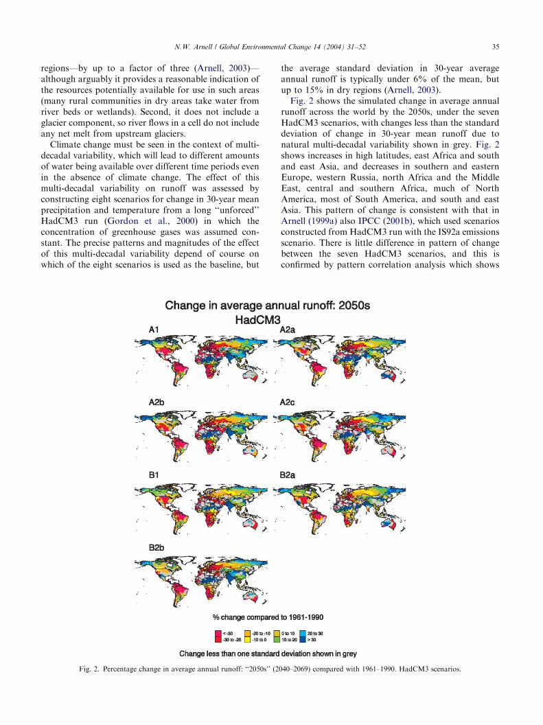
Fig. 2. Percentage change in average annual runoff: ‘‘2050s’’ (2

the average standard deviation in 30-year averageannual runoff is typically under 6% of the mean, butup to 15% in dry regions (Arnell, 2003).Fig. 2 shows the simulated change in average annual

runoff across the world by the 2050s, under the sevenHadCM3 scenarios, with changes less than the standarddeviation of change in 30-year mean runoff due tonatural multi-decadal variability shown in grey. Fig. 2shows increases in high latitudes, east Africa and southand east Asia, and decreases in southern and easternEurope, western Russia, north Africa and the MiddleEast, central and southern Africa, much of NorthAmerica, most of South America, and south and eastAsia. This pattern of change is consistent with that inArnell (1999a) also IPCC (2001b), which used scenariosconstructed from HadCM3 run with the IS92a emissionsscenario. There is little difference in pattern of changebetween the seven HadCM3 scenarios, and this isconfirmed by pattern correlation analysis which shows

040–2069) compared with 1961–1990. HadCM3 scenarios.

ARTICLE IN PRESS

Fig. 3. Percentage change in average annual runoff ‘‘2050s’’ (2040–2069) compared with 1961–1990. A2 scenarios.

N.W. Arnell / Global Environmental Change 14 (2004) 31–5236

that the correlations between the three A2 ensemblemembers or the two B2 ensemble members are generallyno higher than between any pair of scenarios. It wouldbe expected that the changes from the A1FI scenariowould be greater than those from A2 and B2, with thesmallest changes from the B1 scenario. One measure ofthe magnitude of change in runoff is the standarddeviation of change across all watersheds (Arnell, 2003).This shows little systematic difference by the 2020s, andby the 2050s there are only slight indications thatA1FI produces the biggest change and B1 the smallest.By the 2080s the differences between the scenarios areclearer. This implies that until the 2080s, it is possible totreat all seven climate scenarios as members of a singleensemble set.Fig. 3 shows the simulated change in runoff under the

A2 emissions scenario for all six climate models. Thepatterns are, like those for precipitation, broadlysimilar, but with some regional differences. Areas wheremore than half of the simulations show a significantdecrease in runoff (greater than the standard deviationof natural multi-decadal variability) include much ofEurope, the Middle East, southern Africa, NorthAmerica and most of South America. Areas withconsistent increases in runoff include high latitude

North America and Siberia, eastern Africa, parts ofarid Saharan Africa and Australia, and south and eastAsia.

4. Indicators of water resources stress

There is a wide range of potential indicators of waterresources stress, including measures of resources avail-able per person, and populations living in definedstressed categories. This study concentrates on thenumbers of people affected by water resources stress,rather than hydrologically based indicators whichare difficult to compare with those constructed forother impact sectors. There are a number of keyissues associated with the development of appropriateindicators.The first relates to the scale at which the indicators are

calculated. As noted in the introduction, the earliestassessments of global water resources stresses werebased on national scale indices, because that is the levelat which information is generally available. However,national indices can hide very significant sub-nationalvariability, particularly in China, Russia and NorthAmerica, and it is preferable to work at a finer spatial

ARTICLE IN PRESS

Table 3

Water resources index classes

Resources per capita (m3/capita/year)

Index Class

>17001 No stress

1000–1700 Moderate stress

500–1000 High stress

o500 Extreme stress


resolution. Like the Alcamo et al. (2000), PAGE(Revenga et al., 2000) and GEO-3 (UNEP, 2001)studies, the current study calculates indices at the

watershed scale, assuming implicitly that resources in awatershed are equally available throughout that wa-tershed. A number of major world basins are dividedinto several watersheds. In this study, each watershed istreated independently and there is no import of waterfrom upstream watersheds. In practice there will also bedifferent stresses within a watershed. It is possible tocalculate indices at the 0.5� 0.5� scale—both popula-tion and simulated runoff data are available at thatscale—but this will underestimate resource availabilityin areas where large volumes of water are imported fromupstream.The second issue concerns the definition of an

appropriate indicator of pressures on water resources.One widely used indicator is the ratio of withdrawals toaverage annual runoff (as used in the UN Comprehen-sive Assessment of the Freshwater Resources and in theAlcamo et al., 2000, 2003; V .or .osmarty et al., 2000 andGEO-3 studies), but this requires estimates of futurewater withdrawals which will depend not only on futurepopulation but also assumed future water use efficiency.There are currently three global data bases on current

water withdrawals: one developed for the UN Compre-hensive Assessment of the Freshwater Resources of theWorld (Shiklomanov, 1998; Raskin et al., 1997), onepresented in publications of the World ResourcesInstitute (e.g. WRI, 2000) and most recently updatedin Gleick (1998), and one collated by FAO and storedon AQUASTAT (www.fao.org/ag/agl/aglw/aquastat/main/index.shtm). A fourth data set covering 118countries has been prepared at the International WaterManagement Institute (Seckler et al., 1998, 1999).However, due to the use of different baselines and insome cases assumptions, the four data sets rarely givethe same estimates for current water use, with some verylarge differences. Projections of future withdrawals weremade for the UN Comprehensive Assessment (Raskinet al., 1997), by Seckler et al. (1998) and for GEO-3(UNEP, 2001), and again there are substantial differ-ences reflecting different assumptions in particularabout future irrigation use, population growth andwater use efficiency in general. The first two projectionswere based on baseline data from the early 1990s,and in many countries in eastern Europe and centralAsia water withdrawals have fallen substantially sincethen: Moldova’s withdrawals fell by around 50%between 1990 and 1996, for example (UNEP, 1999).Indicators based on estimated future water withdrawalsare therefore highly sensitive to some key, uncertain,assumptions.A second indicator is the amount of water resources

available per person, expressed as m3/capita/year. Theadvantage of this index is that it does not require

assumptions about future water withdrawals: thedisadvantage is that it tends to underestimate stressesin areas where there are very large withdrawals(principally for irrigation). This index was used by thePAGE study (Revenga et al., 2000). The current study

concentrates on resources per capita.The third issue concerns the measure of water

resource availability. The most widely used measure isaverage annual runoff, both generated within the unit ofassessment and imported from upstream. However, insome areas pressures on water resources may bedetermined by the amount of water available in ‘‘dry’’years, and the relationship between mean and extremerunoff varies from region to region (in general, thevariability in runoff from year to year increases as theclimate becomes drier). The current study uses both

average annual runoff and the 10-year return period

minimum annual runoff to characterise available water

resources.The fourth issue concerns the definition of who is water

stressed, and revolves around the specification of criticalthresholds. Table 3 shows a widely used classification ofwater resources stresses (Falkenmark et al., 1989), basedoriginally on a comparison of national resource avail-ability data with an assessment of whether a country wasexperiencing water-related problems. In practice, thethresholds are arbitrary, and all are well above minimumphysiological requirements. The current study assumes

that areas with less than 1000 m3/capita/year are water-

stressed. Revenga et al. (2000) use thresholds of both1700 and 1000m3/capita/year.The final issue relates to the characterisation of the

effects of a change in the amount of resources availableon water resources stresses. A simple measure is thenumber of people who move into, or out of, the water-stressed category. It is not appropriate simply todetermine the net change, because this assumes that‘‘winners’’ exactly compensate ‘‘losers’’, and this is notnecessarily the case: the economic and social costs ofpeople becoming water-stressed are likely to outweighthe economic and social benefits of people ceasing to bewater-stressed (although this suggestion needs furtherinvestigation). Also, the increase in runoff tends to occurduring the wet season, and if not stored will lead to littlebenefit during the dry season, and may be associatedwith an increased frequency of flooding (Arnell, 2003).

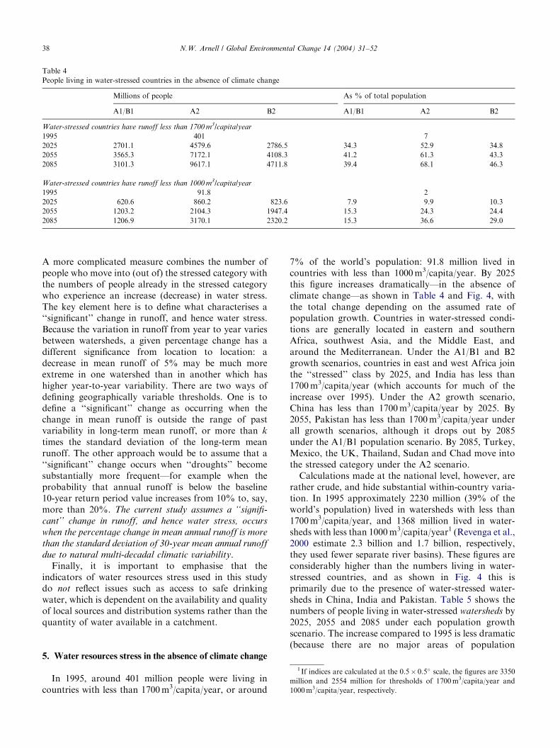
http://www.fao.org/ag/agl/aglw/aquastat/main/index.shtm

http://www.fao.org/ag/agl/aglw/aquastat/main/index.shtm

Table 4

People living in water-stressed countries in the absence of climate change

Millions of people As % of total population

A1/B1 A2 B2 A1/B1 A2 B2

Water-stressed countries have runoff less than 1700 m3/capita/year

1995 401 7

2025 2701.1 4579.6 2786.5 34.3 52.9 34.8

2055 3565.3 7172.1 4108.3 41.2 61.3 43.3

2085 3101.3 9617.1 4711.8 39.4 68.1 46.3

Water-stressed countries have runoff less than 1000 m3/capita/year

1995 91.8 2

2025 620.6 860.2 823.6 7.9 9.9 10.3

2055 1203.2 2104.3 1947.4 15.3 24.3 24.4

2085 1206.9 3170.1 2320.2 15.3 36.6 29.0


A more complicated measure combines the number ofpeople who move into (out of) the stressed category withthe numbers of people already in the stressed categorywho experience an increase (decrease) in water stress.The key element here is to define what characterises a‘‘significant’’ change in runoff, and hence water stress.Because the variation in runoff from year to year variesbetween watersheds, a given percentage change has adifferent significance from location to location: adecrease in mean runoff of 5% may be much moreextreme in one watershed than in another which hashigher year-to-year variability. There are two ways ofdefining geographically variable thresholds. One is todefine a ‘‘significant’’ change as occurring when thechange in mean runoff is outside the range of pastvariability in long-term mean runoff, or more than k

times the standard deviation of the long-term meanrunoff. The other approach would be to assume that a‘‘significant’’ change occurs when ‘‘droughts’’ becomesubstantially more frequent—for example when theprobability that annual runoff is below the baseline10-year return period value increases from 10% to, say,more than 20%. The current study assumes a ‘‘signifi-

cant’’ change in runoff, and hence water stress, occurs

when the percentage change in mean annual runoff is more

than the standard deviation of 30-year mean annual runoff

due to natural multi-decadal climatic variability.Finally, it is important to emphasise that the

indicators of water resources stress used in this studydo not reflect issues such as access to safe drinkingwater, which is dependent on the availability and qualityof local sources and distribution systems rather than thequantity of water available in a catchment.

1 If indices are calculated at the 0.5� 0.5� scale, the figures are 3350

million and 2554 million for thresholds of 1700m3/capita/year and

1000m3/capita/year, respectively.

5. Water resources stress in the absence of climate change

In 1995, around 401 million people were living incountries with less than 1700m3/capita/year, or around

7% of the world’s population: 91.8 million lived incountries with less than 1000m3/capita/year. By 2025this figure increases dramatically—in the absence ofclimate change—as shown in Table 4 and Fig. 4, withthe total change depending on the assumed rate ofpopulation growth. Countries in water-stressed condi-tions are generally located in eastern and southernAfrica, southwest Asia, and the Middle East, andaround the Mediterranean. Under the A1/B1 and B2growth scenarios, countries in east and west Africa jointhe ‘‘stressed’’ class by 2025, and India has less than1700m3/capita/year (which accounts for much of theincrease over 1995). Under the A2 growth scenario,China has less than 1700m3/capita/year by 2025. By2055, Pakistan has less than 1700m3/capita/year underall growth scenarios, although it drops out by 2085under the A1/B1 population scenario. By 2085, Turkey,Mexico, the UK, Thailand, Sudan and Chad move intothe stressed category under the A2 scenario.Calculations made at the national level, however, are

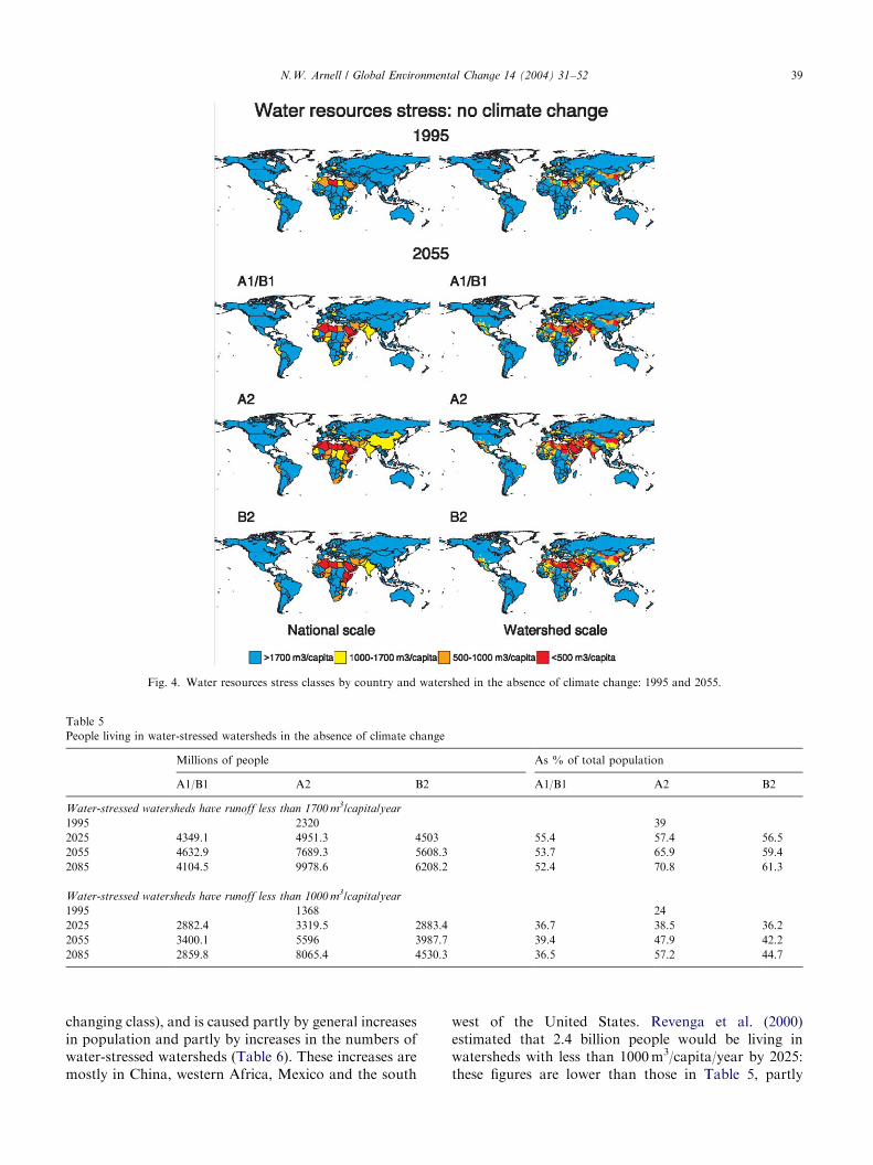
rather crude, and hide substantial within-country varia-tion. In 1995 approximately 2230 million (39% of theworld’s population) lived in watersheds with less than1700m3/capita/year, and 1368 million lived in water-sheds with less than 1000m3/capita/year1 (Revenga et al.,2000 estimate 2.3 billion and 1.7 billion, respectively,they used fewer separate river basins). These figures areconsiderably higher than the numbers living in water-stressed countries, and as shown in Fig. 4 this isprimarily due to the presence of water-stressed water-sheds in China, India and Pakistan. Table 5 shows thenumbers of people living in water-stressed watersheds by2025, 2055 and 2085 under each population growthscenario. The increase compared to 1995 is less dramatic(because there are no major areas of population

ARTICLE IN PRESS

Fig. 4. Water resources stress classes by country and watershed in the absence of climate change: 1995 and 2055.

Table 5

People living in water-stressed watersheds in the absence of climate change


A1/B1 A2 B2 A1/B1 A2 B2

Water-stressed watersheds have runoff less than 1700 m3/capita/year

1995 2320 39

2025 4349.1 4951.3 4503 55.4 57.4 56.5

2055 4632.9 7689.3 5608.3 53.7 65.9 59.4

2085 4104.5 9978.6 6208.2 52.4 70.8 61.3

Water-stressed watersheds have runoff less than 1000 m3/capita/year

1995 1368 24

2025 2882.4 3319.5 2883.4 36.7 38.5 36.2

2055 3400.1 5596 3987.7 39.4 47.9 42.2

2085 2859.8 8065.4 4530.3 36.5 57.2 44.7


changing class), and is caused partly by general increasesin population and partly by increases in the numbers ofwater-stressed watersheds (Table 6). These increases aremostly in China, western Africa, Mexico and the south

west of the United States. Revenga et al. (2000)estimated that 2.4 billion people would be living inwatersheds with less than 1000m3/capita/year by 2025:these figures are lower than those in Table 5, partly


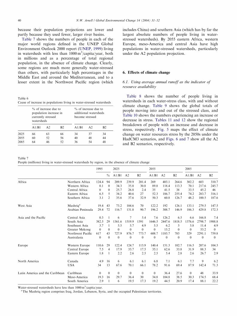
because their population projections are lower andpartly because they used fewer, larger river basins.Table 7 shows the numbers of people in each of the

major world regions defined in the UNEP GlobalEnvironment Outlook 2000 report (UNEP, 1999) livingin watersheds with less than 1000m3/capita/year, bothin millions and as a percentage of total regionalpopulation, in the absence of climate change. Clearly,some regions are much more generally water-stressedthan others, with particularly high percentages in theMiddle East and around the Mediterranean, and to alesser extent in the Northwest Pacific region (which

Table 6

Cause of increase in populations living in water-stressed watersheds

% of increase due to

population increase in

currently stressed

watersheds

% of increase due to

additional watersheds

become stressed

A1/B1 A2 B2 A1/B1 A2 B2

2025 66 63 66 34 37 34

2055 60 52 56 40 48 44

2085 64 46 52 36 54 48

Table 7

People (millions) living in water-stressed watersheds by region, in the absen

1995 2025

% A1/B1

Africa Northern Africa 124.4 94 209.9

Western Africa 0.1 0 34.3

Central Africa 0 0 25.7

Eastern Africa 6.5 5 34.2

Southern Africa 3.1 2 35.6

West Asia Mashriqa 19.4 43 73.2

Arabian Peninsula 29.4 72 116.7

Asia and the Pacific Central Asia 0.3 1 6

South Asia 382.5 29 1361.6

Southeast Asia 3.7 1 5.5

Greater Mekong 0 0 0

Northwest Pacific 617 43 727.9

Australasia 0 0 0

Europe Western Europe 110.6 29 122.4

Central Europe 7.5 4 17.9

Eastern Europe 1.8 1 2.2

North America Canada 4.9 16 6

USA 34 13 67.6

Latin America and the Caribbean Caribbean 0 0 0

Meso-America 19.3 16 29.7

South America 2.9 1 6

Water-stressed watersheds have less than 1000m3/capita/year.aThe Mashriq region comprises Iraq, Jordan, Lebanon, Syria, and the oc

includes China) and southern Asia (which has by far thelargest absolute numbers of people living in water-stressed watersheds). By 2055 eastern Africa, westernEurope, meso-America and central Asia have highpopulations in water-stressed watersheds, particularlyunder the A2 population projection.

6. Effects of climate change

6.1. Using average annual runoff as the indicator of

resource availability

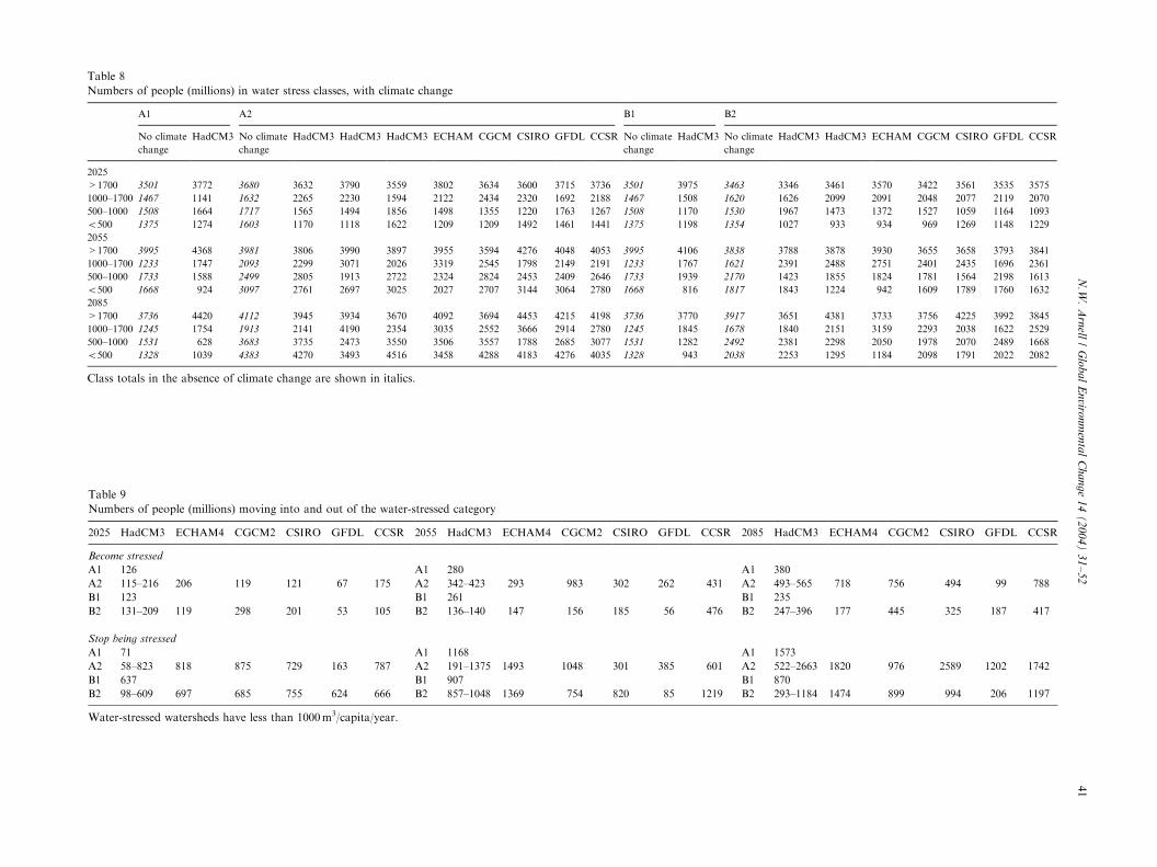
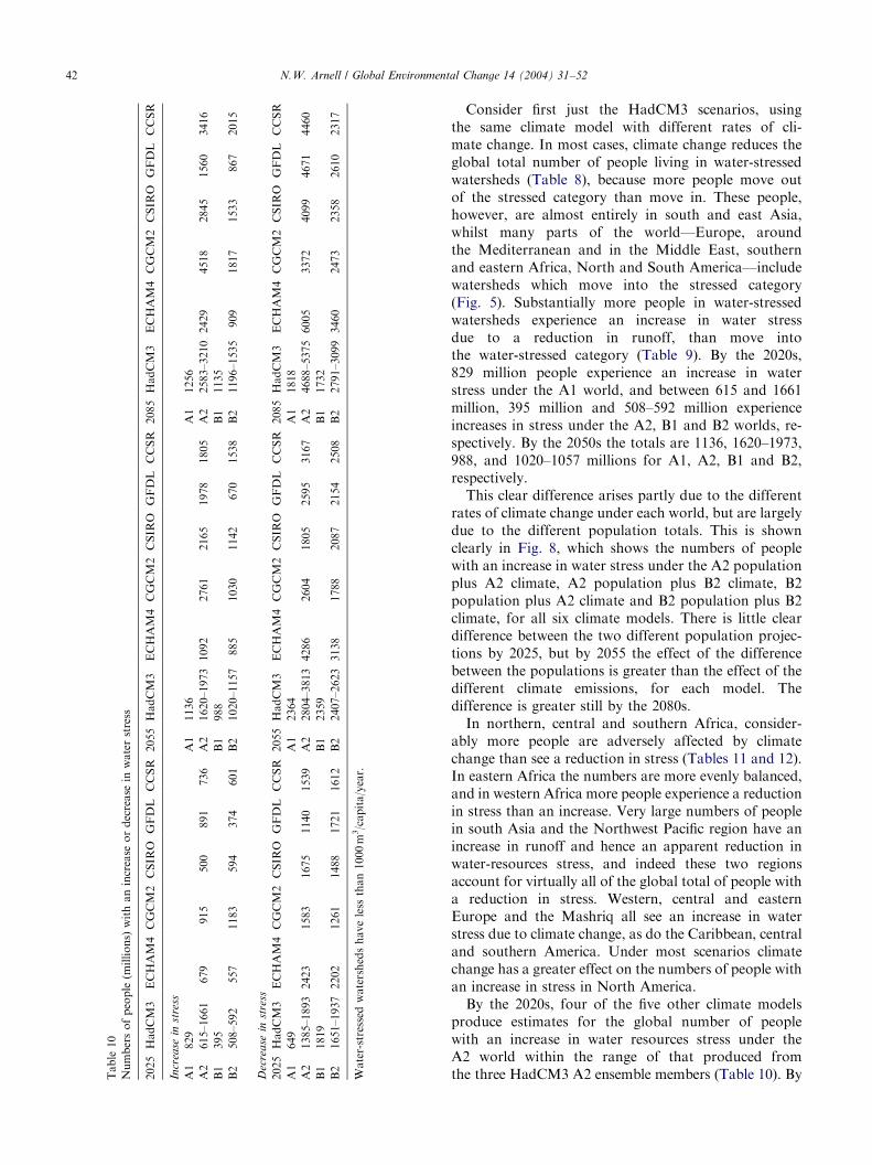
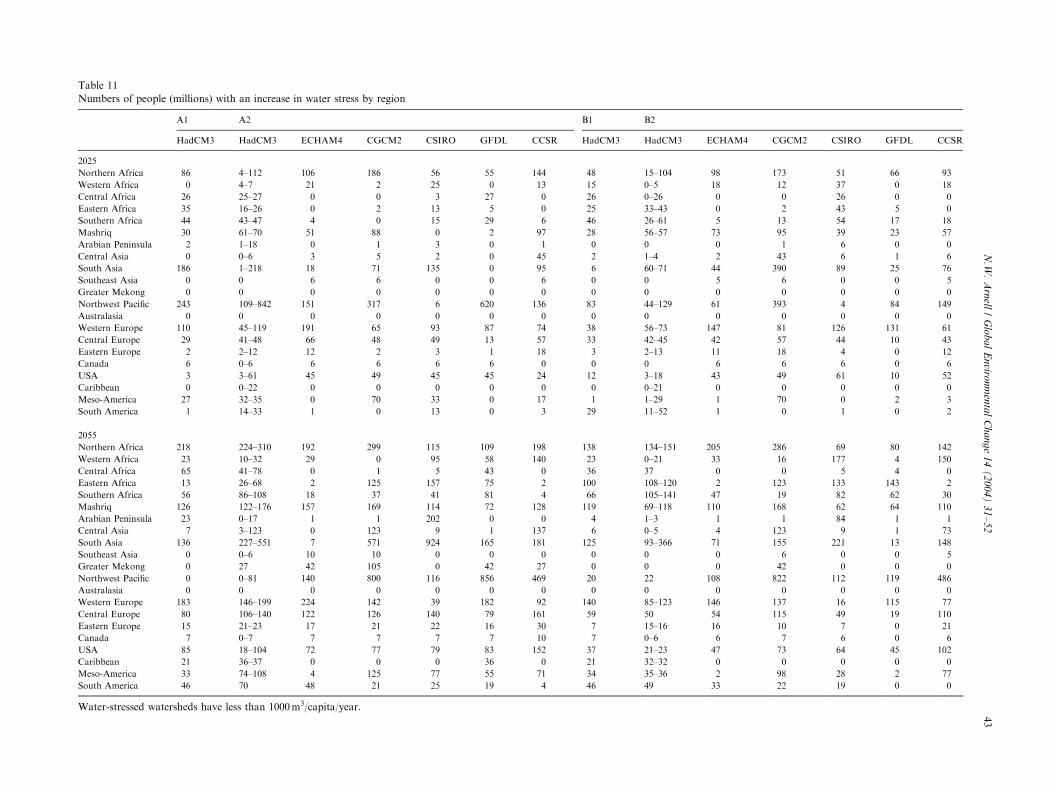
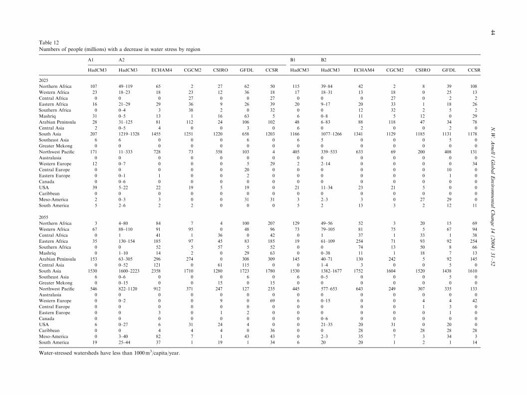
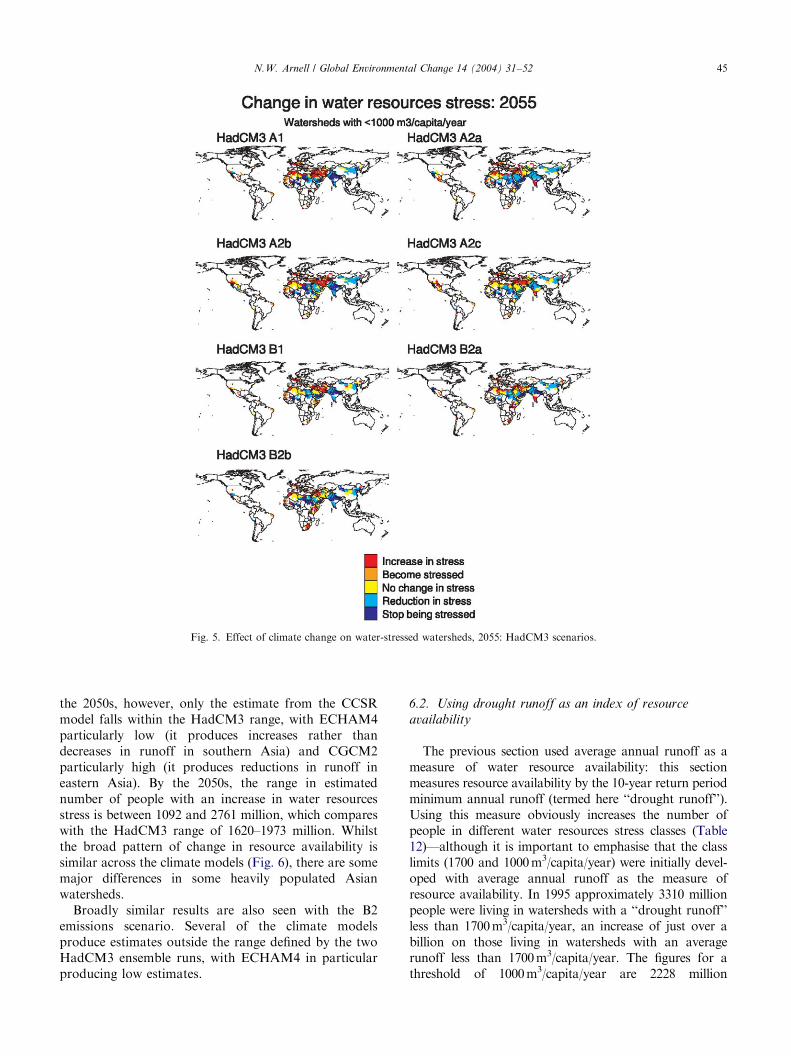
Table 8 shows the number of people living inwatersheds in each water-stress class, with and withoutclimate change. Table 9 shows the global totals ofpeople moving into and out of the stressed class, andTable 10 shows the numbers experiencing an increase ordecrease in stress. Tables 11 and 12 show the regionalbreakdown of people with an increase and decrease instress, respectively. Fig. 5 maps the effect of climatechange on water resources stress by the 2050s under theHadCM3 scenarios, and Figs. 6 and 7 show all the A2and B2 scenarios, respectively.

ce of climate change

2055 2085

A2 B2 A1/B1 A2 B2 A1/B1 A2 B2

239.9 201.4 269 403.1 264.6 302.2 603 310.7

35.8 30.8 89.8 118.4 113.3 70.1 217.6 245.7

26.8 2.4 35 41.5 38 33.5 45.2 46

40.6 27 52.3 186.7 255.4 74.2 283.7 316.1

37.6 32.9 50.3 60.8 126.7 48.2 100.5 187.6

104.6 70 122.2 192 126.1 133.1 279.5 147.5

131.8 90.7 196.2 308.7 146.9 186.3 429.8 172.3

7 5.4 7.6 126.2 6.5 6.6 166.8 7.4

1519.9 1391 1646.5 2447.6 1818.5 1376.6 2798.7 1988.8

5.7 4.9 5.5 6.2 5 5.8 11.4 4.9

0 0 0 15.2 0 0 53.2 0

876.7 773.7 608.7 1185.7 785 329 2291.1 759.8

0 0 0 0 0 0 0 0

124.7 113.9 140.4 151.3 102.7 116.5 207.6 104.3

33.7 17.5 35.1 62.6 33.8 31.9 88.3 34

2.6 2.5 2.5 5.4 2.8 2.6 26.7 2.9

6.1 6.1 6.8 7.1 6.1 7.7 9 6.2

70.1 66.1 78.2 91.6 69.4 87.9 142.4 71.3

0 0 0 36.4 27.6 0 48 33.9

36.4 30 34.8 104.8 38.5 30.3 174.5 68.4

19.5 17.3 19.2 44.5 20.9 17.4 88.1 22.2

cupied Palestinian territories.

ARTIC

LEIN

PRES

STable 8

Numbers of people (millions) in water stress classes, with climate change

A1 A2 B1 B2

No climate

change

HadCM3 No climate

change

HadCM3 HadCM3 HadCM3 ECHAM CGCM CSIRO GFDL CCSR No climate

change

HadCM3 No climate

change

HadCM3 HadCM3 ECHAM CGCM CSIRO GFDL CCSR

2025

>1700 3501 3772 3680 3632 3790 3559 3802 3634 3600 3715 3736 3501 3975 3463 3346 3461 3570 3422 3561 3535 3575

1000–1700 1467 1141 1632 2265 2230 1594 2122 2434 2320 1692 2188 1467 1508 1620 1626 2099 2091 2048 2077 2119 2070

500–1000 1508 1664 1717 1565 1494 1856 1498 1355 1220 1763 1267 1508 1170 1530 1967 1473 1372 1527 1059 1164 1093

o500 1375 1274 1603 1170 1118 1622 1209 1209 1492 1461 1441 1375 1198 1354 1027 933 934 969 1269 1148 1229

2055

>1700 3995 4368 3981 3806 3990 3897 3955 3594 4276 4048 4053 3995 4106 3838 3788 3878 3930 3655 3658 3793 3841

1000–1700 1233 1747 2093 2299 3071 2026 3319 2545 1798 2149 2191 1233 1767 1621 2391 2488 2751 2401 2435 1696 2361

500–1000 1733 1588 2499 2805 1913 2722 2324 2824 2453 2409 2646 1733 1939 2170 1423 1855 1824 1781 1564 2198 1613

o500 1668 924 3097 2761 2697 3025 2027 2707 3144 3064 2780 1668 816 1817 1843 1224 942 1609 1789 1760 1632

2085

>1700 3736 4420 4112 3945 3934 3670 4092 3694 4453 4215 4198 3736 3770 3917 3651 4381 3733 3756 4225 3992 3845

1000–1700 1245 1754 1913 2141 4190 2354 3035 2552 3666 2914 2780 1245 1845 1678 1840 2151 3159 2293 2038 1622 2529

500–1000 1531 628 3683 3735 2473 3550 3506 3557 1788 2685 3077 1531 1282 2492 2381 2298 2050 1978 2070 2489 1668

o500 1328 1039 4383 4270 3493 4516 3458 4288 4183 4276 4035 1328 943 2038 2253 1295 1184 2098 1791 2022 2082

Class totals in the absence of climate change are shown in italics.

Table 9

Numbers of people (millions) moving into and out of the water-stressed category

2025 HadCM3 ECHAM4 CGCM2 CSIRO GFDL CCSR 2055 HadCM3 ECHAM4 CGCM2 CSIRO GFDL CCSR 2085 HadCM3 ECHAM4 CGCM2 CSIRO GFDL CCSR

Become stressed

A1 126 A1 280 A1 380

A2 115–216 206 119 121 67 175 A2 342–423 293 983 302 262 431 A2 493–565 718 756 494 99 788

B1 123 B1 261 B1 235

B2 131–209 119 298 201 53 105 B2 136–140 147 156 185 56 476 B2 247–396 177 445 325 187 417

Stop being stressed

A1 71 A1 1168 A1 1573

A2 58–823 818 875 729 163 787 A2 191–1375 1493 1048 301 385 601 A2 522–2663 1820 976 2589 1202 1742

B1 637 B1 907 B1 870

B2 98–609 697 685 755 624 666 B2 857–1048 1369 754 820 85 1219 B2 293–1184 1474 899 994 206 1197

Water-stressed watersheds have less than 1000m3/capita/year.

N.W

.A

rnell

/G

lob

al

En

viron

men

tal

Ch

an

ge

14

(2

00

4)

31

–5

241

ARTICLE IN PRESS

Table10

Numbersofpeople(m

illions)withanincrease

ordecrease

inwaterstress

2025

HadCM3

ECHAM4

CGCM2

CSIR

OGFDL

CCSR

2055

HadCM3

ECHAM4

CGCM2

CSIR

OGFDL

CCSR

2085

HadCM3

ECHAM4

CGCM2

CSIR

OGFDL

CCSR

Incr

ease

inst

ress

A1

829

A1

1136

A1

1256

A2

615–1661

679

915

500

891

736

A2

1620–1973

1092

2761

2165

1978

1805

A2

2583–3210

2429

4518

2845

1560

3416

B1

395

B1

988

B1

1135

B2

508–592

557

1183

594

374

601

B2

1020–1157

885

1030

1142

670

1538

B2

1196–1535

909

1817

1533

867

2015

Dec

rease

inst

ress

2025

HadCM3

ECHAM4

CGCM2

CSIR

OGFDL

CCSR

2055

HadCM3

ECHAM4

CGCM2

CSIR

OGFDL

CCSR

2085

HadCM3

ECHAM4

CGCM2

CSIR

OGFDL

CCSR

A1

649

A1

2364

A1

1818

A2

1385–1893

2423

1583

1675

1140

1539

A2

2804–3813

4286

2604

1805

2595

3167

A2

4688–5375

6005

3372

4099

4671

4460

B1

1819

B1

2359

B1

1732

B2

1651–1937

2202

1261

1488

1721

1612

B2

2407–2623

3138

1788

2087

2154

2508

B2

2791–3099

3460

2473

2358

2610

2317

Water-stressed

watershedshavelessthan1000m3/capita/year.


Consider first just the HadCM3 scenarios, usingthe same climate model with different rates of cli-mate change. In most cases, climate change reduces theglobal total number of people living in water-stressedwatersheds (Table 8), because more people move outof the stressed category than move in. These people,however, are almost entirely in south and east Asia,whilst many parts of the world—Europe, aroundthe Mediterranean and in the Middle East, southernand eastern Africa, North and South America—includewatersheds which move into the stressed category(Fig. 5). Substantially more people in water-stressedwatersheds experience an increase in water stressdue to a reduction in runoff, than move intothe water-stressed category (Table 9). By the 2020s,829 million people experience an increase in waterstress under the A1 world, and between 615 and 1661million, 395 million and 508–592 million experienceincreases in stress under the A2, B1 and B2 worlds, re-spectively. By the 2050s the totals are 1136, 1620–1973,988, and 1020–1057 millions for A1, A2, B1 and B2,respectively.This clear difference arises partly due to the different

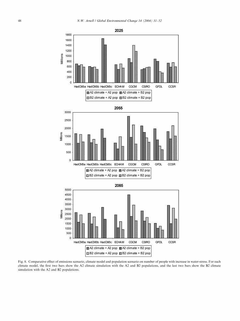
rates of climate change under each world, but are largelydue to the different population totals. This is shownclearly in Fig. 8, which shows the numbers of peoplewith an increase in water stress under the A2 populationplus A2 climate, A2 population plus B2 climate, B2population plus A2 climate and B2 population plus B2climate, for all six climate models. There is little cleardifference between the two different population projec-tions by 2025, but by 2055 the effect of the differencebetween the populations is greater than the effect of thedifferent climate emissions, for each model. Thedifference is greater still by the 2080s.In northern, central and southern Africa, consider-

ably more people are adversely affected by climatechange than see a reduction in stress (Tables 11 and 12).In eastern Africa the numbers are more evenly balanced,and in western Africa more people experience a reductionin stress than an increase. Very large numbers of peoplein south Asia and the Northwest Pacific region have anincrease in runoff and hence an apparent reduction inwater-resources stress, and indeed these two regionsaccount for virtually all of the global total of people witha reduction in stress. Western, central and easternEurope and the Mashriq all see an increase in waterstress due to climate change, as do the Caribbean, centraland southern America. Under most scenarios climatechange has a greater effect on the numbers of people withan increase in stress in North America.By the 2020s, four of the five other climate models

produce estimates for the global number of peoplewith an increase in water resources stress under theA2 world within the range of that produced fromthe three HadCM3 A2 ensemble members (Table 10). By

ARTIC

LEIN

PRES

S

Table 11

Numbers of people (millions) with an increase in water stress by region

A1 A2 B1 B2

HadCM3 HadCM3 ECHAM4 CGCM2 CSIRO GFDL CCSR HadCM3 HadCM3 ECHAM4 CGCM2 CSIRO GFDL CCSR

2025

Northern Africa 86 4–112 106 186 56 55 144 48 15–104 98 173 51 66 93

Western Africa 0 4–7 21 2 25 0 13 15 0–5 18 12 37 0 18

Central Africa 26 25–27 0 0 3 27 0 26 0–26 0 0 26 0 0

Eastern Africa 35 16–26 0 2 13 5 0 25 33–43 0 2 43 5 0

Southern Africa 44 43–47 4 0 15 29 6 46 26–61 5 13 54 17 18

Mashriq 30 61–70 51 88 0 2 97 28 56–57 73 95 39 23 57

Arabian Peninsula 2 1–18 0 1 3 0 1 0 0 0 1 6 0 0

Central Asia 0 0–6 3 5 2 0 45 2 1–4 2 43 6 1 6

South Asia 186 1–218 18 71 135 0 95 6 60–71 44 390 89 25 76

Southeast Asia 0 0 6 6 0 0 6 0 0 5 6 0 0 5

Greater Mekong 0 0 0 0 0 0 0 0 0 0 0 0 0 0

Northwest Pacific 243 109–842 151 317 6 620 136 83 44–129 61 393 4 84 149

Australasia 0 0 0 0 0 0 0 0 0 0 0 0 0 0

Western Europe 110 45–119 191 65 93 87 74 38 56–73 147 81 126 131 61

Central Europe 29 41–48 66 48 49 13 57 33 42–45 42 57 44 10 43

Eastern Europe 2 2–12 12 2 3 1 18 3 2–13 11 18 4 0 12

Canada 6 0–6 6 6 6 6 0 0 0 6 6 6 0 6

USA 3 3–61 45 49 45 45 24 12 3–18 43 49 61 10 52

Caribbean 0 0–22 0 0 0 0 0 0 0–21 0 0 0 0 0

Meso-America 27 32–35 0 70 33 0 17 1 1–29 1 70 0 2 3

South America 1 14–33 1 0 13 0 3 29 11–52 1 0 1 0 2

2055

Northern Africa 218 224–310 192 299 115 109 198 138 134–151 205 286 69 80 142

Western Africa 23 10–32 29 0 95 58 140 23 0–21 33 16 177 4 150

Central Africa 65 41–78 0 1 5 43 0 36 37 0 0 5 4 0

Eastern Africa 13 26–68 2 125 157 75 2 100 108–120 2 123 133 143 2

Southern Africa 56 86–108 18 37 41 81 4 66 105–141 47 19 82 62 30

Mashriq 126 122–176 157 169 114 72 128 119 69–118 110 168 62 64 110

Arabian Peninsula 23 0–17 1 1 202 0 0 4 1–3 1 1 84 1 1

Central Asia 7 3–123 0 123 9 1 137 6 0–5 4 123 9 1 73

South Asia 136 227–551 7 571 924 165 181 125 93–366 71 155 221 13 148

Southeast Asia 0 0–6 10 10 0 0 0 0 0 0 6 0 0 5

Greater Mekong 0 27 42 105 0 42 27 0 0 0 42 0 0 0

Northwest Pacific 0 0–81 140 800 116 856 469 20 22 108 822 112 119 486

Australasia 0 0 0 0 0 0 0 0 0 0 0 0 0 0

Western Europe 183 146–199 224 142 39 182 92 140 85–123 146 137 16 115 77

Central Europe 80 106–140 122 126 140 79 161 59 50 54 115 49 19 110

Eastern Europe 15 21–23 17 21 22 16 30 7 15–16 16 10 7 0 21

Canada 7 0–7 7 7 7 7 10 7 0–6 6 7 6 0 6

USA 85 18–104 72 77 79 83 152 37 21–23 47 73 64 45 102

Caribbean 21 36–37 0 0 0 36 0 21 32–32 0 0 0 0 0

Meso-America 33 74–108 4 125 77 55 71 34 35–36 2 98 28 2 77

South America 46 70 48 21 25 19 4 46 49 33 22 19 0 0


N.W

.A

rnell

/G

lob

al

En

viron

men

tal

Ch

an

ge

14

(2

00

4)

31

–5

243

ARTIC

LEIN

PRES

S

Table 12

Numbers of people (millions) with a decrease in water stress by region

A1 A2 B1 B2

HadCM3 HadCM3 ECHAM4 CGCM2 CSIRO GFDL CCSR HadCM3 HadCM3 ECHAM4 CGCM2 CSIRO GFDL CCSR

2025

Northern Africa 107 49–119 65 2 27 62 50 115 39–84 42 2 8 39 108

Western Africa 23 18–23 18 23 12 36 18 17 18–31 13 18 0 25 13

Central Africa 0 0 0 27 0 0 27 0 0 0 27 0 2 2

Eastern Africa 16 21–29 29 36 9 26 39 20 9–17 20 33 1 18 26

Southern Africa 0 0–4 3 38 2 0 32 0 0 12 32 2 5 2

Mashriq 31 0–5 13 1 16 63 5 6 0–8 11 5 12 0 29


Central Asia 2 0–5 4 0 0 3 0 6 0 2 0 0 2 0

South Asia 207 1219–1328 1455 1251 1220 658 1203 1166 1077–1266 1341 1129 1185 1131 1178

Southeast Asia 6 6 0 0 0 6 0 6 5 0 0 0 5 0

Greater Mekong 0 0 0 0 0 0 0 0 0 0 0 0 0 0


Australasia 0 0 0 0 0 0 0 0 0 0 0 0 0 0

Western Europe 12 0–7 0 0 0 5 29 2 2–14 0 0 0 0 34

Central Europe 0 0 0 0 0 20 0 0 0 0 0 0 10 0

Eastern Europe 0 0–1 1 0 0 2 0 0 0 0 0 0 1 0

Canada 0 0–6 0 0 0 0 0 0 0 0 0 0 0 0

USA 39 5–22 22 19 5 19 0 21 11–34 23 21 5 0 0

Caribbean 0 0 0 0 0 0 0 0 0 0 0 0 0 0

Meso-America 2 0–3 3 0 0 31 31 3 2–3 3 0 27 29 0

South America 5 2–6 2 2 0 0 0 5 2 13 3 2 12 11

2055

Northern Africa 3 4–80 84 7 4 100 207 129 49–56 52 3 20 15 69

Western Africa 67 88–110 91 95 0 48 96 73 79–105 81 75 5 67 94

Central Africa 0 1 41 1 36 0 42 0 1 37 1 33 1 38

Eastern Africa 35 130–154 185 97 45 83 185 19 61–109 254 71 93 92 254

Southern Africa 0 0 52 5 57 5 52 0 0 74 13 50 8 66

Mashriq 0 1–10 14 2 0 29 63 0 0–38 11 1 18 7 13


Central Asia 0 0–52 121 0 61 115 0 0 1–4 3 0 0 5 0

South Asia 1530 1600–2223 2358 1710 1280 1723 1780 1530 1382–1677 1752 1604 1520 1438 1610

Southeast Asia 6 0–6 0 0 0 6 0 6 0–5 0 0 0 5 0

Greater Mekong 0 0–15 0 0 15 0 15 0 0 0 0 0 0 0


Australasia 0 0 0 0 0 0 0 0 0 0 0 0 0 0

Western Europe 0 0–2 0 0 9 0 69 6 0–15 0 0 4 4 42

Central Europe 0 0 0 0 0 0 0 0 0 0 0 1 3 0

Eastern Europe 0 0 3 0 1 2 0 0 0 0 0 0 1 0

Canada 0 0 0 0 0 0 0 0 0–6 0 0 0 0 0

USA 6 0–27 6 31 24 4 0 0 21–35 20 31 0 20 0

Caribbean 0 0 4 4 4 0 36 0 0 28 0 28 28 28

Meso-America 0 3–40 82 7 1 43 43 0 2–3 35 7 3 34 3

South America 19 25–44 37 1 19 1 34 6 20 20 1 2 1 14


N.W

.A

rnell

/G

lob

al

En

viron

men

tal

Ch

an

ge

14

(2

00

4)

31

–5

244

ARTICLE IN PRESS

Fig. 5. Effect of climate change on water-stressed watersheds, 2055: HadCM3 scenarios.


the 2050s, however, only the estimate from the CCSRmodel falls within the HadCM3 range, with ECHAM4particularly low (it produces increases rather thandecreases in runoff in southern Asia) and CGCM2particularly high (it produces reductions in runoff ineastern Asia). By the 2050s, the range in estimatednumber of people with an increase in water resourcesstress is between 1092 and 2761 million, which compareswith the HadCM3 range of 1620–1973 million. Whilstthe broad pattern of change in resource availability issimilar across the climate models (Fig. 6), there are somemajor differences in some heavily populated Asianwatersheds.Broadly similar results are also seen with the B2

emissions scenario. Several of the climate modelsproduce estimates outside the range defined by the twoHadCM3 ensemble runs, with ECHAM4 in particularproducing low estimates.

6.2. Using drought runoff as an index of resource

availability

The previous section used average annual runoff as ameasure of water resource availability: this sectionmeasures resource availability by the 10-year return periodminimum annual runoff (termed here ‘‘drought runoff’’).Using this measure obviously increases the number ofpeople in different water resources stress classes (Table12)—although it is important to emphasise that the classlimits (1700 and 1000m3/capita/year) were initially devel-oped with average annual runoff as the measure ofresource availability. In 1995 approximately 3310 millionpeople were living in watersheds with a ‘‘drought runoff’’less than 1700m3/capita/year, an increase of just over abillion on those living in watersheds with an averagerunoff less than 1700m3/capita/year. The figures for athreshold of 1000m3/capita/year are 2228 million

ARTICLE IN PRESS

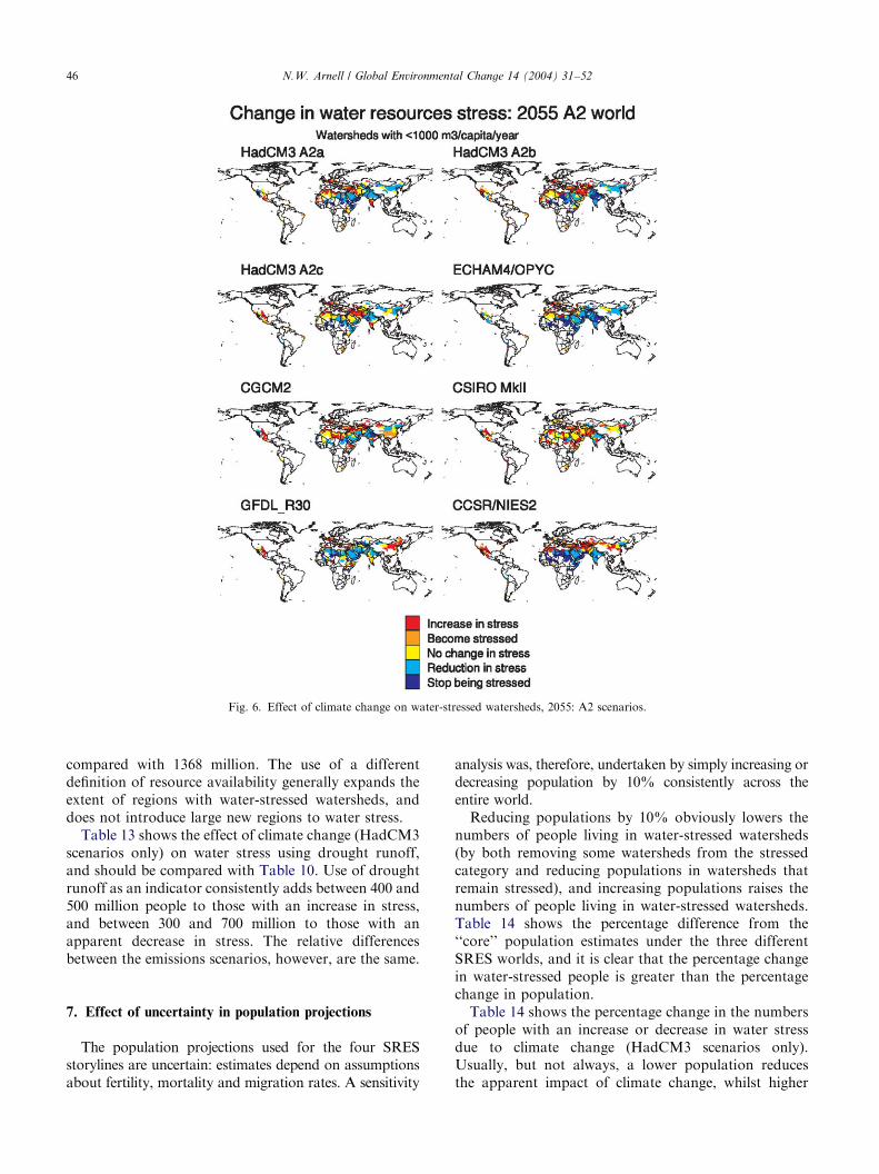
Fig. 6. Effect of climate change on water-stressed watersheds, 2055: A2 scenarios.


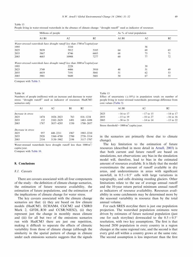
compared with 1368 million. The use of a differentdefinition of resource availability generally expands theextent of regions with water-stressed watersheds, anddoes not introduce large new regions to water stress.Table 13 shows the effect of climate change (HadCM3

scenarios only) on water stress using drought runoff,and should be compared with Table 10. Use of droughtrunoff as an indicator consistently adds between 400 and500 million people to those with an increase in stress,and between 300 and 700 million to those with anapparent decrease in stress. The relative differencesbetween the emissions scenarios, however, are the same.

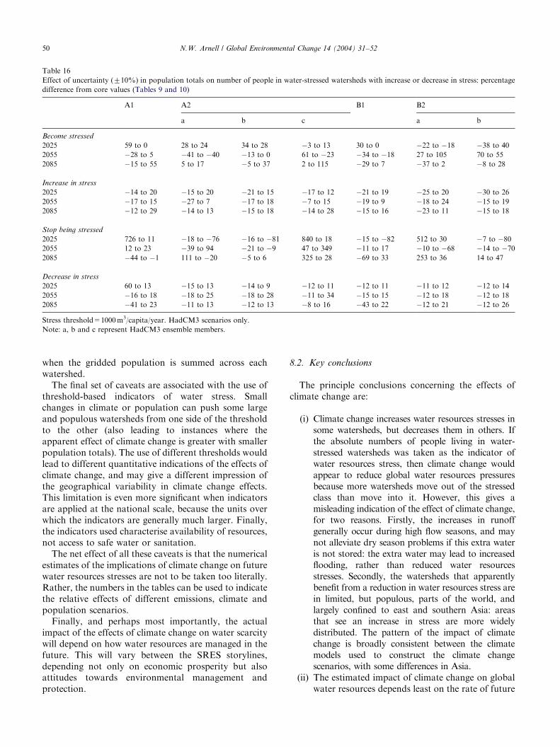
7. Effect of uncertainty in population projections

The population projections used for the four SRESstorylines are uncertain: estimates depend on assumptionsabout fertility, mortality and migration rates. A sensitivity

analysis was, therefore, undertaken by simply increasing ordecreasing population by 10% consistently across theentire world.Reducing populations by 10% obviously lowers the

numbers of people living in water-stressed watersheds(by both removing some watersheds from the stressedcategory and reducing populations in watersheds thatremain stressed), and increasing populations raises thenumbers of people living in water-stressed watersheds.Table 14 shows the percentage difference from the‘‘core’’ population estimates under the three differentSRES worlds, and it is clear that the percentage changein water-stressed people is greater than the percentagechange in population.Table 14 shows the percentage change in the numbers

of people with an increase or decrease in water stressdue to climate change (HadCM3 scenarios only).Usually, but not always, a lower population reducesthe apparent impact of climate change, whilst higher

ARTICLE IN PRESS

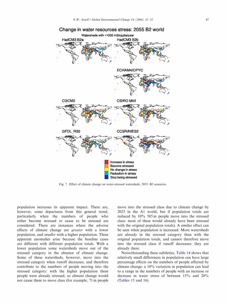
Fig. 7. Effect of climate change on water-stressed watersheds, 2055: B2 scenarios.


population increases its apparent impact. There are,however, some departures from this general trend,particularly when the numbers of people whoeither become stressed or cease to be stressed areconsidered. There are instances where the adverseeffects of climate change are greater with a lowerpopulation, and smaller with a higher population. Theseapparent anomalies arise because the baseline casesare different with different population totals. With alower population some watersheds move out of thestressed category in the absence of climate change.Some of these watersheds, however, move into thestressed category when runoff decreases, and thereforecontribute to the numbers of people moving into thestressed category: with the higher population thesepeople were already stressed, so climate change wouldnot cause them to move class (for example, 71m people

move into the stressed class due to climate change by2025 in the A1 world, but if population totals arereduced by 10% 585m people move into the stressedclass: most of these would already have been stressedwith the original population totals). A similar effect canbe seen when population is increased. More watershedsare already in the stressed category than with theoriginal population totals, and cannot therefore moveinto the stressed class if runoff decreases: they arealready there.Notwithstanding these subtleties, Table 14 shows that

relatively small differences in population can have largepercentage effects on the numbers of people affected byclimate change: a 10% variation in population can leadto a range in the numbers of people with an increase ordecrease in water stress of between 15% and 20%(Tables 15 and 16).

ARTICLE IN PRESS

Fig. 8. Comparative effect of emissions scenario, climate model and population scenario on number of people with increase in water-stress. For each

climate model, the first two bars show the A2 climate simulation with the A2 and B2 populations, and the last two bars show the B2 climate

simulation with the A2 and B2 populations.


ARTICLE IN PRESS

Table 13

People living in water-stressed watersheds in the absence of climate change: ‘‘drought runoff’’ used as indicator of resources


A1/B1 A2 B2 A1/B1 A2 B2

Water-stressed watersheds have drought runoff less than 1700 m3/capita/year

1995 3310 58

2025 5039 5912 5185 64 69 65

2055 5867 8746 6685 68 75 71

2085 4685 10908 7277 60 77 72

Water-stressed watersheds have drought runoff less than 1000 m3/capita/year

1995 2228 39

2025 3749 4406 3910 48 51 49

2055 4419 7191 5041 51 62 53

2085 3901 9449 5601 50 67 55

Compare with Table 5.

Table 14

Numbers of people (millions) with an increase and decrease in water

stress: ‘‘drought runoff’’ used as indicator of resources: HadCM3

scenarios only

A1 A2 B1 B2

Increase in stress

2025 1474 1026–2023 763 816–1234

2055 152 2102–2629 1491 1483–1698

2085 1787 3837–4295 1530 1708–2057

Decrease in stress

2025 957 448–2211 1967 1903–2210

2055 2928 3360–4788 2700 2758–3314

2085 2354 5130–5902 2198 3117–3707

Water-stressed watersheds have drought runoff less than 1000m3/

capita/year.

Compare with Table 10.

Table 15

Effect of uncertainty (710%) in population totals on number of

people living in water-stressed watersheds: percentage difference from

core values (Table 5)

A1/B1 A2 B2

2025 �16 to 17 �17 to 15 �14 to 17

2055 �15 to 19 �18 to 27 �16 to 16

2085 �30 to 21 �14 to 14 �13 to 22

Stress threshold=1000m3/capita/year.


8. Conclusions

8.1. Caveats

There are caveats associated with all four componentsof the study—the definition of climate change scenarios,the estimation of future resource availability, theestimation of future populations, and the estimation ofthe implications of climate change for water stress.The key caveats associated with the climate change

scenarios are that: (i) they are based on few climatemodels (HadCM3, ECHAM4, CGCM2 and CSIROMark 2, GFDL R30 and CCSR/NIES2), (ii) theyrepresent just the change in monthly mean climateand (iii) for all but two of the emissions scenariosrun with HadCM3 there are just one repetition,making it difficult to separate the effects of climaticvariability from those of climate change (although thesimilarity in the spatial pattern of change in climateunder each emissions scenario suggests that the signals

in the scenarios are primarily those due to climatechange).The key limitation to the estimation of future

resources (described in more detail in Arnell, 2003) isthat both current and future runoff are based onsimulations, not observations: any bias in the simulationmodel will, therefore, lead to bias in the estimatedamount of resources available. It is likely that the modeloverestimates the amount of runoff available in dryareas, and underestimates in areas with significantsnowfall, in 0.5� 0.5� cells with large variations intopography, and cells draining receding glaciers. Otherlimitations relate to the use of average annual runoffand the 10-year return period minimum annual runoffas indicators of resource availability. Resources avail-ability in some catchments may be determined more bythe seasonal variability in resource than by the totalannual volume.For each SRES storyline there is just one population

projection. The watershed population estimates weredriven by estimates of future national population (justone for each storyline) downscaled to the 0.5� 0.5�

resolution, with two key assumptions. The first is thatbeyond 2050 population in every country in a regionchanges at the same regional rate, and the second is thatevery grid cell within a country grows at the same rate.The second assumption is less important than the first

ARTICLE IN PRESS

Table 16

Effect of uncertainty (710%) in population totals on number of people in water-stressed watersheds with increase or decrease in stress: percentage

difference from core values (Tables 9 and 10)

A1 A2 B1 B2

a b c a b

Become stressed

2025 59 to 0 28 to 24 34 to 28 �3 to 13 30 to 0 �22 to �18 �38 to 40

2055 �28 to 5 �41 to �40 �13 to 0 61 to �23 �34 to �18 27 to 105 70 to 55

2085 �15 to 55 5 to 17 �5 to 37 2 to 115 �29 to 7 �37 to 2 �8 to 28

Increase in stress

2025 �14 to 20 �15 to 20 �21 to 15 �17 to 12 �21 to 19 �25 to 20 �30 to 26

2055 �17 to 15 �27 to 7 �17 to 18 �7 to 15 �19 to 9 �18 to 24 �15 to 19

2085 �12 to 29 �14 to 13 �15 to 18 �14 to 28 �15 to 16 �23 to 11 �15 to 18

Stop being stressed

2025 726 to 11 �18 to �76 �16 to �81 840 to 18 �15 to �82 512 to 30 �7 to �802055 12 to 23 �39 to 94 �21 to �9 47 to 349 �11 to 17 �10 to �68 �14 to �702085 �44 to �1 111 to �20 �5 to 6 325 to 28 �69 to 33 253 to 36 14 to 47

Decrease in stress

2025 60 to 13 �15 to 13 �14 to 9 �12 to 11 �12 to 11 �11 to 12 �12 to 14

2055 �16 to 18 �18 to 25 �18 to 28 �11 to 34 �15 to 15 �12 to 18 �12 to 18

2085 �41 to 23 �11 to 13 �12 to 13 �8 to 16 �43 to 22 �12 to 21 �12 to 26

Stress threshold=1000m3/capita/year. HadCM3 scenarios only.

Note: a, b and c represent HadCM3 ensemble members.


when the gridded population is summed across eachwatershed.The final set of caveats are associated with the use of

threshold-based indicators of water stress. Smallchanges in climate or population can push some largeand populous watersheds from one side of the thresholdto the other (also leading to instances where theapparent effect of climate change is greater with smallerpopulation totals). The use of different thresholds wouldlead to different quantitative indications of the effects ofclimate change, and may give a different impression ofthe geographical variability in climate change effects.This limitation is even more significant when indicatorsare applied at the national scale, because the units overwhich the indicators are generally much larger. Finally,the indicators used characterise availability of resources,not access to safe water or sanitation.The net effect of all these caveats is that the numerical

estimates of the implications of climate change on futurewater resources stresses are not to be taken too literally.Rather, the numbers in the tables can be used to indicatethe relative effects of different emissions, climate andpopulation scenarios.Finally, and perhaps most importantly, the actual

impact of the effects of climate change on water scarcitywill depend on how water resources are managed in thefuture. This will vary between the SRES storylines,depending not only on economic prosperity but alsoattitudes towards environmental management andprotection.

8.2. Key conclusions

The principle conclusions concerning the effects ofclimate change are:

(i)
Climate change increases water resources stresses insome watersheds, but decreases them in others. Ifthe absolute numbers of people living in water-stressed watersheds was taken as the indicator ofwater resources stress, then climate change wouldappear to reduce global water resources pressuresbecause more watersheds move out of the stressedclass than move into it. However, this gives amisleading indication of the effect of climate change,for two reasons. Firstly, the increases in runoffgenerally occur during high flow seasons, and maynot alleviate dry season problems if this extra wateris not stored: the extra water may lead to increasedflooding, rather than reduced water resourcesstresses. Secondly, the watersheds that apparentlybenefit from a reduction in water resources stress arein limited, but populous, parts of the world, andlargely confined to east and southern Asia: areasthat see an increase in stress are more widelydistributed. The pattern of the impact of climatechange is broadly consistent between the climatemodels used to construct the climate changescenarios, with some differences in Asia.
(ii)
The estimated impact of climate change on globalwater resources depends least on the rate of future

ARTICLE IN PRESSN.W. Arnell / Global Environmental Change 14 (2004) 31–52 51

emissions, and most on the climate model used toestimate changes in climate and the assumedfuture population. By the 2020s between 53 and206 million people move into the water-stressedcategory, and between 374 and 1661 millionpeople are projected to experience an increase inwater stress. There is little difference betweenemissions scenarios and population assumptions,and most of the range derives from the use ofdifferent climate models. By the 2050s there is stilllittle difference between emissions scenario, butthe different population assumptions have a cleareffect. Under the A2 population between 262 and983 million people move into the water-stressedcategory, and between 1092 and 2761 millionpeople have an increase in stress. Under the B2population the ranges are 56–476 million and 670–1538 million respectively, and under the A1/B1population are 261–280 million and 988–1136 (butbased on just one climate model). A change intotal population under a given population scenar-io of plus or minus 10%, for example, leads tochanges in the numbers of people with increases ordecreases in water stress of around 15–20%.

(iii)
Areas with an increase in water resources stressinclude the watersheds around the Mediterranean,in central and southern Africa, Europe, centraland southern America. Areas with an apparentdecrease in water resources stress are concentratedin south and east Asia.
Acknowledgements

This research has been funded by the UK Departmentfor the Environment, Food and Rural Affairs (DE-FRA), contract EPG/1/1/70. Climate baseline data andclimate change scenarios were provided through theClimate Impacts LINK project by Dr. David Viner ofthe Climatic Research Unit, University of East Anglia.The national population projections were provided byCIESIN, New York. Comments from the other mem-bers of the ‘‘Fast Track’’ group and the anonymousreferees are gratefully appreciated.

References

Alcamo, J., D .oll, P., Kaspar, F., Siebert, S., 1997. Global Change and

Global Scenarios of Water Use and Availability: An Application of

WaterGAP1.0. University of Kassel, Germany. 47pp+app.

Alcamo, J., Heinrichs, T., R .osch, T., 2000. World Water in 2025—

Global Modeling and Scenario Analysis for the 21st Century.

Report A0002, Center for Environmental Systems Research,

University of Kassel, Kurt Wolters Strasse 3, Kassel 34109,

Germany.

Alcamo, J., D .oll, P., Heinrichs, T., Kaspar, F., Lehner, B., R .osch, T.,

Siebert, S., 2003. Global estimates of water withdrawals and

availability under current and future business-as-usual conditions.

Hydrological Sciences Journal 48, 339–348.

Arnell, N.W., 1999a. Climate change and global water resources.

Global Environmental Change 9, S31–S49.

Arnell, N.W., 1999b. A simple water balance model for the simulation

of streamflow over a large geographic domain. Journal of

Hydrology 217, 314–335.

Arnell, N.W., 2003. Effect of IPCC SRES emissions scenarios on river

runoff: a global perspective. Hydrology and Earth System Sciences,

submitted for publication.

Arnell, N.W., Livermore, M.J.L., Kovats, S., Nicholls, R., Levy, P.,

et al., 2003. Socio-economic scenarios for climate change impacts

assessments: characterising the SRES storylines. Global Environ-

mental Change 14, 3–20.

Center for International Earth Science Information Network (CIE-

SIN), 2000. Columbia University; International Food Policy

Research Institute (IFPRI); and World Resources Institute

(WRI). 2000. Gridded Population of the World (GPW), Version

2. Palisades, NY: CIESIN, Columbia University; available at

http://sedac.ciesin.columbia.edu/plue/gpw.

Falkenmark, M., Lundquist, J., Widstrand, C., 1989. Macro-scale

water scarcity requires micro-scale approaches: aspects of vulner-

ability in semi-arid development. Natural Resources Forum 13,

258–267.

Gaffin, S.R., Xing, X., Yetman, G., 2003. Downscaling and geo-spatial

gridding of socio-economic projections from the IPCC Special

Report on Emissions Scenarios (SRES), in press.

Gleick, P.H., 1998. The World’s Water: The Biennial Report on

Freshwater Resources 1998–1999. Island Press, San Francisco.

Gordon, C., Cooper, C., Senior, C., Banks, H., Gregory, J.M., Johns,

T.C., Mitchell, J.F.B., Wood, R., 2000. The simulation of SST, sea-

ice extents and ocean heat transports in a version of the Hadley

Centre coupled model without flux adjustments. Climate Dynamics

16, 147–168.

IPCC, 2000. Emissions Scenarios. A Special Report of Working Group

II of the Intergovernmental Panel on Climate Change. Cambridge

University Press, Cambridge.

IPCC, 2001a. Climate Change 2001: The Scientific Basis. Contribu-

tion of Working Group 1 to the Third Assessment Report of

the Intergovernmental Panel on Climate Change. Cambridge


IPCC, 2001b. Climate Change 2001: The Synthesis Report. Cambridge


Johns, T.C., Gregory, J.M., Ingram, W.J., Johnson, C.E., Jones, A.,

Lowe, J.A., Mitchell, J.F.B., Roberts, D.L., Sexton, D.M.H.,

Stevenson, D.S., Tett, S.F.B., Woodage, M.J., 2003. Anthropo-

genic climate change for 1860 to 2100 simulated with the HadCM3

model under up-dated emissions scenarios. Climate Dynamics 20,

583–612.

New, M., Hulme, M., Jones, P.D., 1999. Representing twentieth

century space–time climate variability. Part 1: development of a

1961–1990 mean monthly terrestrial climatology. Journal of

Climate 12, 829–856.

Raskin, P., Gleick, P., Kirshen, P., Pontius, G., Strzepek, K., 1997.

Water Futures: Assessment of Long-range Patterns and Problems.

Background Report for the Comprehensive Assessment of the

Freshwater Resources of the World. Stockholm Environment

Institute: Stockholm, 78pp.

Revenga, C., Brunner, J., Henninger, N., Kassem, K., Payne, N.,

2000. Pilot Analysis of Global Ecosystems: Freshwater Ecosys-

tems. World Resources Institute and Worldwatch Institute,

Washington, DC.

Seckler, D., Amarasinghe, U., Molden, D., de Silva, R., Barker, R.,

1998. World Water Demand and Supply, 1990 to 2025: Scenarios

http://sedac.ciesin.columbia.edu/plue/gpw


and Issues. International Water Management Institute Research

Report 19, Sri Lanka.

Seckler, D., Barker, R., Amarasinghe, U., 1999. Water scarcity in the

twenty-first century. Water Resources Development 15, 29–42.

Shiklomanov, I.A., 1998. Assessment of Water Resources and Water

Availability of the World. Background Report for the Compre-

hensive Assessment of the Freshwater Resources of the World.

World Meteorological Organisation, Geneva.

UNEP, 1999. Global Environment Outlook 2000. Earthscan, London.

UNEP, 2001. Global Environment Outlook-3. Earthscan, London.

V .or .osmarty, C.J., Green, P.J., Salisbury, J., Lammers, R.B., 2000.

Global water resources: vulnerability from climate change and

population growth. Science 289, 284–288.

World Meteorological Organisation, 1997. A comprehensive assess-

ment of the freshwater resources of the world. WMO: Geneva.

World Resources Institute, 2000. World Resources 2000–2001. People

and Ecosystems: The Fraying Web of Life. World Resources

Institute, Washington.

climate change and global water resources: sres emissions and

Documents