1

Responding to Climate Change: the need for a paradigm shift

Diane L. Douglas, Ph.D., RPA

Abstract Global warming is one of the most important and dangerous issues facing man today. Many scientists and politicians have focused on anthropogenic causes of this change and the need to reduce CO2 emissions to limit or slow the process. Major climate changes, however, have occurred throughout earth’s history. The shifting of continental plates, rise of mountains, and cyclical changes in earth’s orbit around the sun are primary forcing mechanisms driving climate change. The complex coupling between the atmosphere, ocean, clouds, ice sheets, volcanoes, earthquakes, and the exchange of carbon within living organisms also affect climate. Over the past two million years, earth’s climate has been punctuated by glacial and interglacial periods—periods when earth’s temperature ranged from 8oC cooler to 4oC warmer than present. Hominids adapted their settlements and subsistence practices to these changes. Modern humans evolved around 40,000 years ago, during the last ice age, and at the end of the last ice age migrated to new lands and new continents. People developed new technologies and adaptive strategies in response to sea level rise and a more productive environment. Today we face climate change of a similar magnitude to the last interglacial. This paper shows how natural forcing mechanisms may drive earth into an interglacial as warm as the last interglacial, regardless of reductions in greenhouse gas emissions. Sea level may rise 4.6 – 6 m (15 – 20 ft), and in some regions storms will increase in frequency and strength, and in others deserts will expand. In order to plan appropriate responses climate change we must first obtain a comprehensive understanding of natural forcing mechanisms and how anthropogenic activities accentuate these mechanisms. At present there are two schools of thought: 1) anthropogenic burning of fossil fuels and land use practices are driving global warming; and 2) earth is experiencing a natural climate cycle, similar to cycles that have occurred in the past. The first argument is dismissed by some as being too simplistic—earth’s climate is driven by complex dynamics and recent warming can not be entirely explained by anthropogenic emissions of CO2 and other greenhouse gases. The second argument is dismissed by others because the rate of global warming observed in the past fifty years exceeds warming documented in historic records, or reconstructed further back in history using proxy data. This paper discusses the current state of scientific knowledge of global warming, and argues that the current state of knowledge is inadequate for developing reliable estimates of future climate change. The technical reports prepared by the intergovernmental panel for climate change (IPCC) are reviewed, gaps in knowledge identified by these authors are discussed, and recommendations for future research are proffered.

2

Table of Contents Abstract ........................................................................................................................................... 1 Introduction..................................................................................................................................... 3

Organization of this Paper .......................................................................................................... 5 The Global Warming Debate .......................................................................................................... 6 Earth’s Energy Balance................................................................................................................... 9

Variation in Earth’s Energy Balance ........................................................................................ 10 Photosynthesis....................................................................................................................... 10 CO2 Pressure in the Ocean versus Atmosphere .................................................................... 11 Albedo................................................................................................................................... 11 Tectonics and Volcanism...................................................................................................... 12 Atmospheric Circulation....................................................................................................... 15 Intertropical Convergence Zone (ITCZ)............................................................................... 16 Oceanic Circulation .............................................................................................................. 17 Changes in Atmospheric and Oceanic Circulation ............................................................... 18 Temporal Variations in Atmospheric and Oceanic Circulation............................................20 Celestial Mechanics .............................................................................................................. 20

Climate Models............................................................................................................................. 24 The IPCC Climate Models........................................................................................................ 26 Climate Models of the Past for Predicting the Future............................................................... 27

IPCC and Ocean Acidity....................................................................................................... 29 Verifying Climate Models ........................................................................................................ 30

Reconstructing Past Environments to Predict the Future ............................................................. 32 Proxy Data ................................................................................................................................ 32

Tree Rings as Proxy Data ..................................................................................................... 35 Pollen as Proxy Data............................................................................................................. 36 Macrobotanical Materials as Proxy Data.............................................................................. 36 Isotopes as Proxy Data.......................................................................................................... 38

Proxy Data Limitations............................................................................................................. 41 Limitations of Tree-Rings and Macrobotanical Data ........................................................... 42 Limitations of Isotopes: Ice Cores and Foraminifera........................................................... 42

Archaeology, History and Climate Change .................................................................................. 46 Economics of Greenhouse Gas Policies ....................................................................................... 47 Discussion..................................................................................................................................... 48

Punctuated Equilibrium and the Threshold Effect.................................................................... 49 Research Suggestions.................................................................................................................... 51

Paleoenvironmental Reconstructions........................................................................................ 51 Modeling................................................................................................................................... 52

Conclusions................................................................................................................................... 52 References..................................................................................................................................... 54 Appendix 1.................................................................................................................................... 66 Climate Models and Their Parameters.......................................................................................... 66

3

Introduction

Global warming is one of the most important and dangerous issues facing man today. Many

scientists and politicians have focused on anthropogenic causes of this change and the need to

reduce CO2 emissions to limit or slow the process. For several years, many scientists have

argued that anthropogenic greenhouse gas (GHG) emissions and land use practices are the

primary forcing mechanism driving current global warming. The idea that people are the primary

cause of global warming as observed in worldwide temperature records is based on reports from

the Intergovernmental Panel of Climate Change (ICPP). The IPCC was established in 1988 by

the United Nations Environment Programme (UNEP) and the World Meteorological

Organization (WMO), both of which are a part of the United Nations (IPCC 2008). This

organization was formed to review and summarize climate studies that analyze the affects of

anthropogenic GHG emissions, including carbon dioxide (CO2), methane (CH4), nitrous oxide

(N2O) and various chlorofluorocarbons (CFCs), and human land use on climate change. Human

land use is an important consideration in climate change studies because deforestation removes

trees and plants that convert CO2 to oxygen (O2) through photosynthesis.

In order to understand how different trace gases affect global warming, the heat potential of CO2,

CH4, N2O and CFC and other miscellaneous gases have been analyzed (United States

Department of Energy (DOE) 2000). The analysts determined that CO2 has the highest potential

for retaining heat, and that relative to other trace gases in the atmosphere it contributes 72.34% to

global warming. The IPCC reports indicate that anthropogenic emissions of CO2 is increasing

the %age of CO2 in the atmosphere, which is causing the atmosphere to warm at a faster rate

than would occur under natural conditions (Forster et al. 2007; Jansen et al. 2007; Randall et al.

2007). Because CO2 retains considerably more heat than CH4, N2O or CFCs, the IPCC has

warned policymakers that if anthropogenic emissions of CO2 are not reduced and maintained at

levels pre-dating 1990, the earth will warm by up to 6.1oC between 2060 and 2090 (Barker et al.

2007:39). Warming of this magnitude replicates the degree of warming that scientists have

determined occurred during the last interglacial period, between 125,000 and 115,000 years ago.

Sea level during this period was approximately 5m (16 ft) higher than present—a level that will

result in devastating flooding of major coastal cities such as Venice, Italy, New York, New York,

and St. Petersburg, Florida. In addition to these heavily populated areas, many coastal natural

world heritage sites that contribute to earth’s rich biodiversity and beauty will be inundated.

World heritage cultural sites located along coastlines subjected to erosion and intense storms will

also be destroyed and lost to future generations.

In addition to direct impacts on coastal cities, estuaries, beaches and cultural sites, warming of

this magnitude has the potential to affect changes in atmospheric and oceanic circulation,

4

resulting in more intense storms in some regions and drought in others. Changes in atmospheric

and oceanic circulation will also affect the distribution of arable lands and the distribution of

shellfish, fish, and other marine organisms that people rely upon for food. The IPCC panel

predicts devastating effects to the world economy as a result of stresses to global food and

potable water supplies, and social and political stresses associated with the need to relocate

millions of people from coastal communities and low-lying islands.

The economic and social implications of global warming have spurred policymakers to request

guidance from economists and scientists on how to slow, and ultimately stop global warming.

To return CO2 in the atmosphere to pre-1990 levels, governments of developed nations have

invested billions of dollars to identify the technological means to reduce global greenhouse gas

emissions. Nearly all of the member nations of the United Nations have ratified the Kyoto

Protocol, a measure established by the United Nations Framework Convention on Climate

Change (UNFCCC) which legally binds ratifying countries to control their GHG emissions

(UNFCCC 2008). To achieve this goal, however, several billion more dollars will need to be

spent to develop new sources of energy and modify industry, vehicles, and homes to be more

energy efficient. In the United States alone it is estimated that the cost to ratify the Kyoto

Protocol would be approximately 400 hundred billion dollars and result in a loss of roughly 4.9

million jobs (Daynes and Sussman 2006). Further, consultants to UNEP report that in response to

climate change over $ 210 billion dollars will be invested annually by 2030 to mitigate and

develop a sustainable energy supply infrastructure (UNEP 2008:9). Given the financial cost of

responding to global warming, communities worldwide can hope that the Kyoto Protocol and

other measures being implemented to reduce anthropogenic GHG emissions and minimize

deforestation will have a significant impact on slowing and/or stopping global warming.

The current worldwide recession makes it clear that the world’s financial resources are limited,

and we must be efficient and effective in our actions to combat and respond to global warming.

Some scientists argue, however, that we are not adequately considering natural forcing

mechanisms that may be the underlying cause of much of the global warming observed in recent

decades. The scientific studies reviewed and reported upon by the IPCC Fourth Working Group

(Barker et al. 2007; IPCC 2007a and IPCC 2007b; Jansen et al. 2007; Forster et al. 2007; Randall

et al. 2007), document multiple areas where the research reviewed does not conclude with

certainty that anthropogenic GHG emissions and land use practices are the primary forcing

mechanism causing recent global warming. These scientists note that additional research must be

performed to understand the complex interaction of anthropogenic behavior and natural forcing

mechanisms (Jansen et al. 2007; Randall et al. 2007; Meehl et al. 2007). For example, the

climate models used to simulate future climate could not fully integrate natural climate forcing

mechanisms because of time and cost constraints, as well as limited knowledge of some physical

5

processes (Jansen et al. 2007; Randall et al. 2007). The Fourth Working Group technical reports

were summarized by the IPCC (e.g., Barker et al. 2007; IPCC 2007a and 2007b). Although these

summaries recognize uncertainties in the technical reports, they state that the scientific evidence

overwhelmingly indicates people are having a significant impact on global warming; these

reports are being used to guide the UNFCCC on how global climate change should be addressed

(Barker et al. 2007; IPCC 2007a and 2007b).

This paper summarizes the current state of knowledge of climate change based on the IPCC

technical reports (Forster et al. 2007; Jansen et al. 2007; Randall et al. 2007), as well as

independent studies (e.g. Hirst 1999; Giorgi and Mearns 2001; Freidenreich and Ramaswamy

2005; Gregory et al. 2005; Hall et al. 2005; Berger et al. 2006). Gaps in knowledge regarding

global climate change identified by these scientists are summarized. Natural forcing mechanisms

that may be contributing to the rapid climate change observed over the past 50 years are

highlighted (e.g. Trogler et al. 1997; Patterson 2005), and additional research that might fill the

data gaps identified by the IPCC are discussed. In addition to the IPCC technical reports, over

150 scientific papers were reviewed by the author of this paper in an effort to bridge the gap

between what is known about anthropogenic forcing of global warming and natural forcing of

global warming. The author’s intent is to highlight areas where additional research is needed to

better understand the natural mechanisms that are accentuating anthropogenic affects of climate

change. This research was performed to inform policymakers that the current approaches to

combating and responding to global warming may not be sufficient to prepare world

communities to climate change that may be imminent. The author’s objective is to provide

policymakers with information that can be used to direct use of the world’s limited financial

resources more efficiently and effectively than is currently planned. No money was accepted

from any parties for the research or writing of this report—additionally the report was prepared

by the author on time off from work and does not reflect the views of her employer.

Organization of this Paper

This paper places anthropogenic causes of global within the context of natural forcing

mechanisms that have driven climate change over millions of years. The first section of the

paper summarizes the history of socio-political and scientific concerns regarding the impacts of

anthropogenic aerosol pollutants on human health and the environment. The next section

discusses the balance between incoming solar radiation from the sun and outgoing long wave

radiation emitted from earth, and highlights how earth’s atmosphere functions. The following

section summarizes the physical processes that affect climate variability on different temporal

and spatial scales. The next section explains how information on earth’s physical dynamics is

used to develop climate models that reconstruct past climates and simulate future climate change.

6

Methods used to verify the accuracy and reliability of these models is then reviewed. The next

section discusses climate models used by the IPCC Fourth Working Group to simulate climate

change under different socio-economic and technological scenarios (Randall et al. 2007).

Inadequacies of these models to predict future climate change is also summarized (Randall et al.

2007). The following section summarizes the types of environmental data (proxy data) used to

verify models of past climates (Jansen et al. 2007) and the limitations of these data for

reconstructing climate conditions at different temporal and spatial scales (Schwander and

Stauffer 1984; Mix and Ruddiman 1984; Stauffer et al. 1985; Mix 1987; Barnola et al. 1991;

Petit et al. 1999; Jansen et al. 2007; Fontanier et al 2008). Following this the economic and social

implications of global warming induced by anthropogenic and natural forcing mechanisms are

discussed (Forster et al. 2007; IPCC 2007; Meehl et al. 2007). Finally, research that could

provide greater understanding of the magnitude of current global warming caused by natural

forcing mechanisms is proposed.

The Global Warming Debate Scientists first became concerned that anthropogenic activities were having an adverse effect on

the atmosphere in the 1950s when they began identifying adverse affects of anthropogenic

aerosols (CO2, CH4, N2O and CFCs) on human health, agricultural productivity and livestock. In

response to this discovery, the United States Congress passed the Air Pollution Control Act

(1955, public law 84-159) and over the next eight years implemented two amendments,

encouraging additional research on the impacts of aerosols on human health and the

environment. In 1963 the United States Congress passed the Clean Air Act (public law 88-206)

and granted 95 million dollars to conduct additional research and develop programs to control

aerosol emissions. Over the next 27 years, scientists identified increasing adverse effects of air

pollutants to human health and the environment (American Meteorological Society 2008). Prior

to publicity regarding the effects of anthropogenic GHG emissions on global warming, the most

widely publicized discovery was the affect of CFCs on the ozone layer. This layer of natural

atmospheric gas (O3) is located in the stratosphere and absorbs approximately 95% of the sun’s

ultraviolet light, which can cause an increase in skin cancer, as well as damage livestock, crops,

plankton and algae. When policymakers became aware of the imminent threat on human life, the

U.S. Congress amended the Clean Air Act (1990, public law 101-549) and mandated adoption of

best available control technologies to reduce CFC emissions.

Around this same time, the UNEP and WMO formed the IPCC to study the extent to which

human land use practices and anthropogenic GHG emissions are causing global warming (IPCC

2009). Since 1988, the IPCC has performed an extensive review of scientific studies on climate

change and prepared exhaustive reports detailing the results of these reviews. The IPCC is

7

organized into three working groups, one which summarizes the physical sciences of climate

change, another which summarizes the vulnerability of human and natural systems to climate

change, and a third which evaluates mitigation measures to reduce or control GHG emissions

(IPCC 2009). It is important to note that these scientists do not perform independent research,

but rather review the results of studies performed by other scientists.

The first IPCC technical report series was released in 1990, and its findings were key in

establishing the Intergovernmental Negotiating Committee (INC) for the United Nations

Framework Convention on Climate Change (UNFCCC). The IPCC’s second report was released

in 1995, and their statement that, “[t]he balance of evidence suggests a discernible human

influence on global climate,” contributed significantly to the formation and adoption of the

Kyoto Protocol (IPCC 2009). The third and fourth assessment reports, released in 2001 and

2007 respectively, contributed even more to the perception that human land use (deforestation,

desertification, draining of wetlands, and expansion of cities) and anthropogenic GHG emissions

from industry and vehicles are major forcing mechanisms in global warming.

Based on the early findings of the IPCC, the United Nations gave the UNFCCC the task of

promoting the adoption of best available control technologies to reduce GHG emissions. Within

a few years of being formed, 192 of the member nations of the United Nations ratified the

UNFCCC and pledged to limit or reduce their GHG emissions. The release of the first IPCC

reports made scientists and policymakers aware of the amounts of anthropogenic GHG emissions

being emitted into the atmosphere relative to natural volumes of GHG emissions and the

UNFCCC adopted more extreme measures to reduce anthropogenic GHG emissions. In 1997 the

UNFCCC adopted the Kyoto Protocol which legally binds ratifying countries to control their

GHG emissions (UNFCCC 2008).

Concurrent with the IPCC investigations of human-induced global warming, other climate

scientists have argued that anthropogenic GHG emissions contribute less than 1% to global

warming, and that natural and anthropogenic CO2 combined contribute only 3.62% to

greenhouse warming (Trogler et al. 1997; Patterson 2005). Chemical analyses of the heat

retention characteristics of atmospheric trace gases and water vapor have determined that the

heat retention characteristics of water vapor are much higher than that of CO2 (see the United

States Department of Energy [DOE] 2000); atmospheric physicists note that water vapor retains

95% of the heat in the atmosphere (Trogler et al. 1997). Based on these findings, and the fact that

CO2 comprises less than 0.04% of the atmosphere and water vapor comprises 1% several

scientists have argued that changes in the amount of water vapor in the atmosphere must be

8

driving the rate and magnitude of global warming that has occurred since AD 1850 (see for

example Trogler et al. 1997; Essenhigh 2001; Jaworowski 2004; Patterson 2005).

However, the arguments presented by these scientists are often dismissed without serious

consideration, their critics claiming that the research performed by these scientists must have

been financed by big industry, biasing their results (Gore 2006; Michaels 2008, Reinhard 2008).

However, the much of the data reported upon by these scientists are derived from United States

federal agencies, and these data are available to the public (and scientists) for review,

consideration and analysis. These agencies include the: National Oceanic and Atmospheric

Administration (NOAA); National Center for Atmospheric Research (NCAR); Carbon Dioxide

Information Analysis Center of the United States DOE; and National Aeronautics and Space

Administration (NASA). Public links for these organizations and their data are presented in the

references section of this paper; these data were used by the author to develop several of the

graphs and charts presented in this paper.

Dismissing the arguments of climate scientists who state earth’s natural forcing mechanisms are

the primary cause of global warming out-of-hand does not do justice to the scientific process.

Perhaps more critically, it suggests policymakers are not giving full consideration to the natural

forcing mechanisms driving global warming. The statements made by these scientists should be

evaluated with the rigor applied to the scientific studies reviewed and reported upon by the

IPCC. The IPCC’s “role is to assess on a comprehensive, objective, open and transparent basis

the latest scientific, technical and socio-economic literature produced worldwide relevant to the

understanding of the risk of human-induced climate change” (IPCC 2009, emphasis added).

Relative to this mandate, the IPCC reports are extremely comprehensive (Forester et al. 2007;

Jansen et al. 2007; Randall et al. 2007; Meehl et al. 2007).

However, given that the policies adopted by the world’s leading nations will affect all life on

earth as well as the global economy for generations to come, perhaps natural forcing mechanisms

should be given full consideration in the analysis of climate change: present and future. These

natural mechanisms combined with anthropogenic effects may result in even more extreme

conditions than the UNFCCC and its member nations are currently considering. Earth’s physical

processes and the dynamics of earth’s energy balance that drive the CO2 cycle and climate

change are very complex, as are the climate models that are used to simulate climate change.

Below, the physical processes that drive earth’s energy balance are reviewed to provide a

framework for understanding natural forcing mechanisms that drive climate change. This

information provides a context for understanding the additional research that the IPCC Fourth

Working Group identifies as necessary for developing a more comprehensive understanding of

climate change.

9

Earth’s Energy Balance

Life on earth would not be possible without the energy received from the sun and the life-giving

air of our atmosphere. Earth’s atmosphere is composed of nitrogen (78.8%), oxygen (20.95%),

argon (0.93%), carbon dioxide (0.038%), various other trace gases and water vapor (1%). The

molecules associated with these gases have mass. Correspondingly, because of the effect of

gravity air is denser closer to the earth (such as at sea level) than it is higher in the atmosphere

(such as on top of Mount Everest). Understanding atmospheric pressure is important for

understanding climate change on seasonal to millennial time scales, because it affects how warm

air is distributed from the equator to the poles, as well as how warm and cold air is distributed

across continents. In climatology, air density is measured by atmospheric pressure and at sea

level mean atmospheric pressure is about 101300 pascals (1013 millibars: mbar). On top of

Mount Everest, roughly 8.9 kilometers (5.5 miles) above sea level, mean atmospheric pressure is

about 34000 pascals (340 mbar) (West 1999). Atmospheric pressure also varies temporally and

spatially across the globe in response to variations in incoming solar radiation and oceanic

circulation. These changes in atmospheric pressure cause changes in regional weather, including

everything from droughts, thunderstorms and tornadoes to hurricanes and monsoon rains.

The energy received from the sun as short wave radiation (insolation) is in delicate balance with

the energy emitted by earth as outgoing long wave radiation (Figure 1). The average amount of

energy received at the top of the atmosphere from the sun is approximately 1,366 watts per

square meter (W/m2), with the highest levels of radiation received at the equator. A marked

increase or decrease in insolation effects earth’s climate, and is the primary reason earth

experiences ice ages (glacial periods) and interglacial periods, such as today. Approximately 19

% of the sun’s shortwave radiation is absorbed by the earth’s atmosphere, and 51% is absorbed

by the land and water bodies (Pidwirny 2006a and 2006b); the remaining short wave radiation

(30%) is reflected back to space by particles in the atmosphere, clouds, and earth’s albedo.

Figure 1. Earth’s Energy Balance.

10

For earth’s heat budget to remain in balance, the amount of incoming solar radiation absorbed by

the atmosphere and earth (70%) must be balanced by the same amount of outgoing longwave

radiation (70%). Radiation emitted by the earth is called longwave radiation because it is cooler

than the sun and emits longer wavelengths of energy. Approximately 70% of the longwave

radiation emitted by earth passes through the atmosphere and escapes to space. The remaining

30% is trapped by water vapor and aerosols (trace gases) in the atmosphere and warms the

earth—this is referred to as the greenhouse effect. The greenhouse effect makes life on earth

possible, but changes in the amount of aerosols and/or water vapor in the atmosphere can have a

marked effect on climate. Higher levels of trace gases (greenhouse gases) trap more longwave

radiation and effectively heat earth’s surface; a reduction in the levels of greenhouse gases

allows more long-wave radiation to escape, effectively cooling earth’s surface.

Variation in Earth’s Energy Balance

Variation in earth’s energy balance occurs over long and short time scales and in response to

multiple variables including changes in: 1) the amount of incoming solar radiation 2) earth’s CO2

cycle – photosynthesis and diffusion into the ocean, 3) albedo, 4) tectonic and volcanic activity,

5) atmospheric and oceanic circulation and 6) celestial mechanics. The contribution of each of

these systems to earth’s energy balance is discussed in greater detail below.

Photosynthesis

Energy from the sun drives photosynthesis in all land plants, algae and some types of

photosynthetic bacteria (Whitmarsh and Govinjee 1999). Photosynthesis converts CO2 from the

air and water (H2O) into O2 and carbohydrates (C6H12O6); O2 is utilized by all oxygen

consuming organisms on earth (Whitmarsh and Govinjee 1999:11). Deforestation and land

clearing therefore result in less CO2 being absorbed by plants, throwing off the natural balance of

earth’s CO2 cycle.

Whitmarsh and Govinjee (1999), note that absorption of CO2 by planktonic foraminifera in the

upper layers of the oceans removes approximately 2 x 1015 grams of carbon per year from the

atmosphere. The process is initiated by plankton photosynthesizing CO2 into organic carbon

(Whitmarsh and Govinjee 1999), as well as CO2 and H2O reacting to form HCO3 (carbonate

ions) which is absorbed by marine organisms to form shells of calcium carbonate (CaCO3). As

these organisms die, they sink to the bottom of the ocean where they settle into the sediment

(Whitmarsh and Govinjee 1999).

11

The ocean contains approximately 19 and 50 times more CO2 than the terrestrial biosphere,

atmosphere, respectively (Sabine 2008). In Polar waters, CO2 absorption is highest during the

summer when the Arctic regions are blanketed in flora; absorption decreases during winter

because of ice cover (Tans et al. 1990; Primack 2004).

CO2 Pressure in the Ocean versus Atmosphere

In addition to CO2 being absorbed by planktonic foraminifera, CO2 is absorbed by the upper

layers of the ocean when the CO2 gas pressure (pCO2) in the atmosphere is higher than the pCO2

in the ocean’s upper layers (Sabine 2008). In high latitudes, CO2 flows from the atmosphere into

the ocean and in the tropics CO2 is released from the ocean to the atmosphere through

evaporation (Glushkov et al. 2005). Large shifts in CO2 concentrations in the oceans occurs

horizontally and vertically as a result of the slow rate of mixing by volume; the concentration of

dissolved CO2 is approximately 10 % higher by volume in the deep ocean than it is at the surface

(Sabine 2008).

Albedo

Albedo refers to the absorptive and reflectivity properties of clouds, the ocean and various

landforms to incoming solar radiation. Light colored surfaces such as snow reflect the greatest

amount of radiation back to space, whereas dark surface like asphalt absorb a lot of solar

radiation. Human land use practices affect earth’s albedo because development, deforestation,

desertification, agriculture and grazing livestock (a few of many human activities) change the

absorptive and reflective properties of earth’s surface. These activities therefore have a direct

affect on earth’s energy balance. Deforestation also affects the amount of vegetation available to

absorb CO2 and convert it to O2, through photosynthesis, which as described above, also affects

earth’s energy balance.

Different types of clouds have different physical properties which affect whether the cloud

absorbs or reflects short wave and long wave radiation. Stratocumulus clouds, which are low

thick clouds, cool the earth’s surface by reflecting short wave radiation back to space. In

contrast, high altitude cirrus clouds warm the atmosphere because they transmit incoming solar

radiation to earth’s surface and also reflect outgoing long wave radiation back to earth (NASA

2007). There is seasonal and regional variability in the cooling versus heating effect of clouds on

the global energy balance, and NASA scientists (2007) note that the effects of low and high

altitude clouds on climate generally balance each other out; the cooling effect of low altitude

clouds is slightly stronger than the warming effect of high altitude clouds, however (NASA

2007).

12

Tectonics and Volcanism

Throughout earth’s history, levels of CO2 in the atmosphere has varied, ranging from over 3000

parts per million by volume (ppmv) to about 100 ppmv (Pagani et al. 2005). Extreme variations

in atmospheric CO2 have occurred in response to natural geologic and biological processes (e.g.,

Pearson and Palmer 2000; Berner and Kothavala 2001; Obzhirov et al. 2003; Cardellini et al.

2004; Pagani et al. 2005; Spence and Telmer 2005; Gurrieri et al. 2006). During the late

Paleocene and early Eocene, roughly 60 to 50 million years ago, atmospheric levels of CO2

ranged from 1000 to 1500 ppmv and during this period, temperate forests extended to the poles

and tropical climates extended to 45o N latitude (Pagani et al. 2005). Today only herbs, grasses,

forbs, sedges and stunted trees grow at high latitudes due to lower insolation levels, and arid

grasslands and temperate forests grow where tropical forests once thrived. The high levels of

atmospheric CO2 during this period are attributed to volcanism in East Greenland (Pagani et al.

2005) and potentially a massive release of methane from the disturbance of organic matter buried

on the sea floor as the result of an earthquake or mudslide (Venere 2006).

This period in earth’s geologic history is known as the Paleocene-Eocene Thermal Maximum

(PETM). The high CO2 levels of this geologic time in earth’s history, combined with increased

CO2 levels during the PETM led to acidification of the ocean, a 6o C to 7o C rise in high latitude

temperatures and contributed to the extinction of dinosaurs (Storey et al. 2007). Over the next

several million years, atmospheric CO2 gradually decreased with this trace gas reaching modern

levels by the late Oligocene (33.7 to 23.8 million years ago). Retallack et al. (2004: 817) note

that several factors may have contributed to this decrease in atmospheric CO2 including changes

in oceanic circulation associated with movement of continental plates, weathering associated

with mountain building, and the expansion of grassland and grazers into formerly forested areas.

Others note that a massive bloom of water ferns (Azolla) and subsequent die off resulted in a

drawdown of atmospheric CO2 from roughly 3000 ppmv to 650 ppmv, as the dead ferns sank to

the sea floor and became incorporated into deep sea sediments—known as the Azolla event

(Dickens et al. 1997; Pagani et al. 2005). The expansion of temperate forests during the Miocene

(23.03 to 5.33 million years ago) resulted in a further drawdown of atmospheric CO2 from 650

ppmv to 100 ppmv. After this period, earth’s plates continued to shift and mountains formed in

New Zealand and Europe affecting atmospheric and oceanic circulation. During the Miocene

earth began to experience ice ages, but the extreme glacial events of the Quaternary period

(starting 1.8 million years ago) would not occur for several million years. Atmospheric CO2 is

typically lower during glacial periods than during interglacial periods because ice sheets cover

areas that are blanketed with flora during interglacial periods.

13

Shifts in the location of tectonic plates, affects atmospheric and oceanic circulation which affects

climate and the CO2 balance; small scale movements (earthquakes) also affect earth’s CO2

balance. Seismic slipping along fault lines can cause supersaturation of CO2 in the melted

sediment/rock. Infrared analysis of friction induced melts in rock, caused by seismic slipping

along the Nojima fault during the 1995 Kobe earthquake (Japan), indicate 1.8 to 3.4 thousand

tons of CO2 were released by the earthquake (Famin et al. 2007). Similarly, geochemical analysis

of water from springs located near active faults in the Gulf of Corinth, Greece (Pizzino et al.

2004) revealed high levels of dissolved CO2 for 1 to 10 months following earthquakes (Famin et

al. 2007).

Volcanism also affects the amount of CO2 in the atmosphere, but generally leads to hemispheric

cooling rather than heating because sulfur dioxide (SO2) is the primary gas released, not CO2

(Gerlach 1990, 1991; Halmer et al. 2002) (Figure 2). When Mount Pinatubo erupted in 1991, 14

to 26 million tons of SO2 were released to the atmosphere.

Figure 2. Satellite Photograph of an Exploding Volcano (from NOAA 2009a).

The SO2 combined with the haze created by the volcanic ash and dust cooled the atmosphere by

0.5oC for a period of 12 to 18 months, ameliorating any warming caused by emission of CO2 to

the atmosphere. However, active volcanic regions release CO2 to the atmosphere through

volcanic vents (fumaroles) and porous soil, even when the volcano is quiescent (USGS 2008).

For example, Ajuppa et al. (2004) studied rates of CO2 degassing on the flanks of the Somma-

Vesuvius volcano and found that soil CO2 concentrations ranged from 50 to 10,500 ppmv. In

another study, Favara et al. (2001) analyzed the amount of CO2 degassing from soils and vents

on Pantelleria Island, an active volcanic complex, to determine how much CO2 is emitted from

the soils, water and fumeroles on the island. These scientists found that 1.79 million metric tones

of CO2 was degassing from the soil, water and fumeroles on the island.

14

The emissions of SO2 and CO2 from terrestrial and marine volcanoes are significant sources of

trace gases into the atmosphere. Because of their threat to human life, as well as their impact on

climate, terrestrial volcanoes are extensively studied (USGS 2008). However, 70 % of

volcanic activity occurs along deep sea rifts located over one mile below the surface of the

ocean, and the effect these marine volcanoes have on earth’s climate is poorly understood

(NOAA 2009a). Because deep sea volcanoes have a significant impact on the global chemical

and heat balance, the NOAA established a program dedicated to studying deep sea hydrothermal

systems: Pacific Marine Environmental Laboratory (PMEL). In 2004, PMEL scientists studying

hydrothermal vents along the Mariana Arc in the North Pacific Ocean (Figure 3) discovered a

vent emitting a wide stream of effervescent bubbles (Lupton and Butterfield 2004). They

captured a sample of the liquid (Figure 4.) in containers and brought these to the surface for

analysis. Lupton and Butterfield (2004) identified 2.3 moles (101g) of gaseous CO2 per liter of

hot water recovered from the vent. The rate in which CO2 is released from one section of the

vent over a period of one day may be comparable to the rate of flow from a water hose. It is

estimated that 30 liters of water flows from an average backyard water hose (1.6 cm diameter)

every minute. If the amount of CO2 emitted from a 1.6 cm2 section of the hydrothermal vent was

constant for 24 hours this area would emit 4,300 metric tonnes of CO2 in one day. If a single 1.6

cm2 area of a vent released liquid CO2 year round, 9 million metric tonnes of CO2 would be

released from this small area in one year. Given there are almost 22,000 kilometers (~12,000

miles) of volcanic arcs along the ocean floor that are not well studied, this system could be

contributing significant levels of CO2 to the ocean and atmosphere.

Figure 3. Earth’s Plate Boundaries: The Mariana Arc (from NOAA 2009).

15

Figure 4. Photograph of Hydrothermal Vent Emitting Liquid CO2 (from NOAA 2009).

Atmospheric Circulation

The majority of the sun’s incoming solar radiation is received at the equator and this heat is

transported to the poles by atmospheric circulation. The Hadley cell (0 to 30o N/S), Ferrell cell

(30 to 60o N/S), and Polar cell (90 to 60o N/S) drive large scale atmospheric circulation and

distribute heat from the equator to the Poles (Figure 5). High pressure systems dominate the

Hadley cell between 20 and 40o N/S, and the Polar cell between 70 to 90o N/S. These systems

Figure 5. Schematic cross-section of earth’s atmospheric circulation cells.

16

form when dry air converges high in the atmosphere creating a parcel of air with higher pressure

than the surrounding atmosphere. The parcel of dry air sinks to earth’s surface creating some of

earth’s largest deserts. The Gobi (Asia), Great Victoria (Australia), Kalahari and Sahara (Africa)

and Sonoran (North America) occur in a band between 20 and 40o N/S. The Polar cell is also

comprised of dry air and as such the Arctic and Antarctic are considered polar deserts.

In contrast to areas of high pressure, low pressure systems dominate where moist air rises near

the equator and between 40 and 60o N/S. Low pressure systems form when air diverges in the

upper atmosphere creating a vacuum that draws in surface air. Air rushes in to fill the vacuum

created by a low pressure system. As the air rises it cools and condenses creating clouds and

precipitation. When extreme low pressure systems form over warm-ocean water the surrounding

air spirals in generating hurricanes and cyclones, such as hurricane Katrina (Handwerk 2005) and

tropical storm Kammuri (Bradhere 2008).

In addition to pressure (temperature) differences between the equator and poles driving

atmospheric circulation, physical forces associated with earth’s rotation on its axis affects

circulation. The force of earth spinning causes winds in the atmosphere to be deflected away

from the equator (Coriolis force). Winds associated with high pressure systems are deflected

clockwise in the Northern Hemisphere and counterclockwise in the Southern Hemisphere

(NASA 2007). Winds associated with low pressure systems are deflected counterclockwise in

the Northern Hemisphere and clockwise in the Southern Hemisphere. The Coriolis force also

results in the formation of earth’s prevailing winds: the Westerlies, Polar easterlies, Doldrums,

Horse latitudes and Trade Winds.

Intertropical Convergence Zone (ITCZ)

Seasonal changes in the location of the solar zenith effects shifts in the location of the Hadley,

Ferrell and Polar cells; the shift is greatest near the equator creating the Intertropical

Convergence Zone (ITCZ). The ITCZ is an area of low pressure that forms where the Northeast

Trade Winds meet the Southeast Trade Winds near the earth's equator. As these winds converge,

moist air is forced upward—as the air cools it condenses and creates a heavy band of

precipitation—the ITCZ also affects the duration and intensity of monsoon rains. In response to

changes in the location of the solar zenith, the ITCZ shifts from approximately 25 o N in

Northern Hemisphere summer (June-July-August) to 20o S in Southern Hemisphere summer

(November-December-January); the shift in the ITCZ results in monsoons in each hemisphere

(Gordon 2000).

17

Oceanic Circulation

Like the atmosphere, oceanic circulation distributes heat from the equator to high latitudes in

currents driven by earth’s prevailing winds, the Coriolis force and differences in the salinity

(density) of the water (Gross 1993). Because large scale ocean circulation is driven by

differences in temperature and salinity it is referred to as thermohaline circulation. The upper

400 meters of the ocean is also driven by prevailing winds in the atmosphere and wind driven

currents are critical to the movement of warm equatorial surface waters to higher latitudes

(Figure 6). The Gulf Stream, originating in the Gulf of Mexico is the largest surface current on

earth (NOAA 2009c). The Gulf Stream carries warm, relatively fresh water along the eastern

coast of North America to northern Newfoundland where it is deflected east by the Coriolis force

and flows to the mid-Atlantic ocean. West of Ireland, the current splits with one branch flowing

north and another south. The northern branch becomes a broad, shallow swath of warm water

called the North Atlantic Drift Current (NADC) which carries warm saline water to the North

Atlantic, moderating the climate of Europe and western Scandinavia. The southern branch of the

current joins the southward flowing Canary Current, which is wide, slow moving current that

flows south to Senegal where it is deflected west (Rossby 1996 and 1999).

Figure 6. Oceanic Circulation: Earth’s Thermohaline Belt (from NOAA,2009).

18

A similar circulation system occurs in the Pacific Ocean. The Kuroshio Current is akin to the

Gulf Stream, originating near Taiwan it flows north along the coast of Asia carrying warm water

to the North Pacific Ocean. The current is deflected west north of Japan and becomes a broad

swath of warm water moving east. In the eastern North Pacific Ocean the current splits into a

northern and southern branch. The northern branch, the Alaska Current carries warm waters

north and the southern branch, the California Current, carries cooler waters south.

The surface and deep water currents of the oceans form the Meridonal Overturning Circulation

(MOC) system. Surface currents are driven by wind, whereas deep ocean currents are driven by

differences in temperature and salinity. In the North Atlantic, the warm surface water condenses

when it encounters colder air causing seasonal fog, rain and snow in Europe and Scandinavia (a

similar system exists in the North Pacific Ocean). The colder, highly saline water left behind is

dense and sinks to depths of 1500 to 2500 m (4900 to 8200 ft), forming the North Atlantic Deep

Water (NADW) current. The NADW flows south along the coasts of the Americas finally

deflecting east near the tip of South America to join the Antarctic Circumpolar Current (ACC).

The ACC flows along the northern edge of Antarctica until it splits into two branches off the tip

of South Africa. One branch flows north into the Indian Ocean and another continues east along

the Antarctic coast until it reaches the Pacific Ocean. Here the current deflects and flows north

off the New Zealand coast and ultimately into the North Pacific Ocean (Smith et al. 2008).

In the North Pacific, this cold, deep current gradually mixes with overlying warmer surface water

and forms into a surface current deflected to the southwest and into the Indonesian Ocean. The

current continues a westward path, with branches entering the Indian and Atlantic oceans. As it

reaches the Atlantic Ocean, the current is deflected north and ultimately returns to the North

Atlantic Ocean where it once again mixes with cold, saline water, sinks and the conveyor-belt

cycle begins again. Oceanic models indicate it takes approximately 1000 years for a parcel of

water within the conveyor belt to complete one cycle from the North Atlantic Ocean to the North

Pacific Ocean and back to the North Atlantic Ocean (Doney et al. 2006).

Changes in Atmospheric and Oceanic Circulation

Changes in the volume and temperature of the Gulf Stream and Kuroshio Current can cause

significant changes in regional weather in the North Pacific Ocean and North Atlantic. Seasonal

changes in regional sea surface temperature as well as shifts in the location and intensity of

surface ocean currents and deep water upwelling cause changes in regional and global climate

(Broeker 1997; Little et al. 1997; Doney et al. 2006; Randall et al. 2007; NOAA 2009c). These

are referred to as coupled ocean-atmosphere circulation systems and shifts in these systems can

19

have dramatic effects on the intensity and duration of droughts in some regions and storms in

others. Systems that are tracked by NOAA include the: Pacific North American (PNA)

Oscillation, Arctic Oscillation (AO), North Atlantic Oscillation (NAO), El Nino/Southern

Oscillation (ENSO), and Antarctic Oscillation (AAO) (NOAA 2006b).

The location and intensity of weather patterns associated with each of these systems is driven by

the location and intensity of the high and low pressure systems that drive them (Randall et al.

2007; NOAA 2009b), as well as the influence of surface currents and NADW (Schiller et al.

1997; Bischoff et al. 2003). For example, the strength of the NAO is directly affected by the

warmth and volume of the Gulf Stream current (Saunders and Qian 2001; NOAA 2009b).

Variation in the NAO effects winter weather in Europe and the UK (Saunders and Qian 2002). A

moderately negative NAO leads to colder, drier, and calmer winters than average in northwest

Europe and warmer and wetter winters in southern Europe (Saunders and Qian 2001). A

moderately positive NAO results in wetter, stormy winters than average in northwest Europe,

and cold dry winters in southern Europe (Saunders and Qian 2001).

Like the NAO, variation in ENSO can significantly influence weather patterns in different

regions. Warm ENSO events (El Niño) occur when sea surface temperatures (SST) are

unusually warm in the central and east-central equatorial Pacific (Figure 7). El Niño events

typically result in above average precipitation in California and Mexico and drought in eastern

Australia (NOAA 2009b). Cool ENSO events (La Niña) occur when SST in the equatorial

pacific are unusually cool and result in above average precipitation in the Northwest of North

America, dry conditions in California and Mexico and increased rains in eastern Australia

(NOAA 2009b).

Figure 7. El Niño Southern Oscillation: El Niño and La Niña (from NOAA 2009b).

20

Temporal Variations in Atmospheric and Oceanic Circulation

Changes in atmospheric and oceanic circulation driven by low frequency changes in earth orbit

around the sun (celestial mechanics: see below) contributed to earth’s glacial and interglacial

periods. Little et al. (1997) speculated that at different times in the past, intensified trade winds,

forced a higher volume of warm tropical and subtropical waters across the equator and into the

Gulf Stream. As this large body of warm water moved into the North Atlantic it cooled and

condensed resulting in increased precipitation/ snow, enhancing the growth of ice-sheets and

potentially contributing to the onset of ice ages (Broecker 1997; Little et al. 1997;; Clark et al.

2002; Manabe and Stouffer 1988, 1997; Manabe et al. 1991; Vellinga and Wood 2002;

Stoufferand Manabe 2003). Near the end of interglacial periods, it is conceivable that heat

stored in the atmosphere and ocean over thousands of years drives more intensive tropical and

subtropical storms resulting in more fresh water being dumped into the Gulf Stream through

runoff and precipitation (Douglas 1989). Over several years, the repeated influx of low-saline

water from the Gulf Stream into the Atlantic Ocean would dilute the cold, high-saline Arctic

waters, potentially causing the MOC to shut down (Douglas 1989). Shutting down the MOC

would cause water from the Gulf Stream to pool in the North Atlantic, causing higher levels of

precipitation and stronger storms in Western Europe and Scandinavia. This precipitation and

cooler temperatures would enhance the growth of alpine glaciers and ice sheets in these regions.

Additionally, because fresh water freezes at a higher temperature than salt water 0o C versus -1.9o

C to -19o C, respectively (the temperature at which sea water freezes varies considerably,

contingent upon the level of salinity, wind sheer, current strength), sea ice could form more

readily as a result of an influx of less saline water to the Arctic via the Gulf Stream (see for

example Frey et al. 2003).

Celestial Mechanics

The astronomical theory developed by Milutin Milankovitch in the early 1900s is widely

accepted by climate scientists as the best theory for explaining changes in the seasons, as well as

climate change over hundreds of thousands of years (Milankovitch 1941; Kerr 1987).

Milankovitch identified seasonal and longer-term systematic variations in earth’s orbit around

the sun based on meticulous measurements on the position of stars and equations that explained

how the gravitational pull of other planets and stars affected earth’s orbit. Through his

calculations, Milankovitch identified three primary celestial mechanisms that affect long-term

cycles of cooling and warming on earth including eccentricity, precession of the equinox and

obliquity. Each of these is discussed in greater detail below.

21

Eccentricity refers to a systematic shift in earth’s orbit around the sun from an eclipse to a

circular pattern and back to an eclipse every 95,000 to 136,000 years, averaging 100,000 years

(Figures 8 and 9). The shape of earth’s orbit around the sun affects how close the earth is to the

Figure 8. Schematic of Variation in Earth’s Axial Tilt (from NOAA 2009).

22

Figure 9. Schematic of Precession (from NOAA 2009).

23

sun on its annual cycle. When earth’s orbit is circular, its distance from the sun is relatively

steady throughout the year, minimizing extreme seasonal variation. When earth’s orbit is

eccentric, seasonal variation in temperature is more extreme. In an eccentric orbit, the earth is

closest to the sun at perihelion and farthest from the sun at aphelion. If perihelion occurs during

northern hemisphere summer this accentuates the length and intensity of the summer season. If

aphelion occurs during northern hemisphere summer, the season is shorter and less intense.

Precession refers to a wobble of the earth in its orbital path around the sun that occurs every

19,000 to 23,000 years (refer to Figure 9). This wobble affects the point when earth’s orbit is

nearest the sun (the location of perihelion), and shifts from the northern to the southern

hemisphere approximately every 9,500 to 11,500 years. Changes in earth’s orbital cycle

(eccentric or round) accentuate the affect of precession on hemispheric warming and cooling

(Imbrie and Imbrie 1980; Bradley 1985; Kutzbach 1987).

Obliquity refers to the earth rotating on an axis that is tilted at an oblique angle to the plane of

ecliptic (Figure 9); the angle of earth’s tilt varies from 22.3 to 24.5o every 41,000 years. This tilt

is what causes the seasons; northern hemisphere summer occurs when the North Pole is tilted

toward the sun, and southern hemisphere summer occurs when the South Pole is tilted toward the

sun. Seasons can be accentuated or modified by eccentricity and precession.

Astronomical theory suggests that cyclic changes in earth’s orbital parameters accentuates

seasons and contributes to the onset of glacial and interglacial periods. Examination of the

mathematical components of eccentricity, obliquity and precession reveal several components

that suggest periodic movement of a wave in a fixed frequency and wavelength (Imbrie and

Imbrie 1980). As such, changes in earth’s orbital parameters can be calculated over the past

several million years as well as into the future (Imbrie and Imbrie 1980). The mathematical

certainty of earth’s orbital parameters allows climate scientists to use the calculations to

reconstruct the timing of glacial and interglacial periods, as well as predict future climate driven

by celestial mechanics (e.g., Ruddiman et al. 2005; Douglas 2007a and 2007b; Stuckless and

Levitch 2007) (Figure 10). However, Imbrie and Imbrie (1980) caution that celestial mechanics

explain only 25% of climate change, noting that other natural forcing mechanisms and feedbacks

drive 75 % of climate change.

24

Figure 10. Reconstruction of Insolation (400,000 years to present) based on Earth’s Orbital Parameters (from NOAA 2009).

Climate Models Over the past thirty years, scientists have developed models to simulate changes in earth’s

climate on global (Muller 1997; Muller et al. 1997; Lopez et al. 2006), hemispheric (Kutzbach

1987) and regional scales (Giorgi and Francisco 2000a and 2000b), based on celestial mechanics

and other natural forcing mechanisms. Models utilized by climate scientists vary in their

resolution and sophistication. Common models used to better understand past glacial and

interglacial periods as well as predict future climate include: earth system models of intermediate

complexity (EMICs), general circulation models (GCMs), and atmospheric-ocean general

circulation models (AOGCM) (see Figures 11, 12 and 13 for images of climate models) (Randall

et al. 2007).

Climate models are based on the fundamental laws of physics, such as Fourier’s law of heat

conduction (heat moves matter (or air) from an area of higher temperature to an area of lower

temperature), or Newton’s laws of motion (Randall et al. 2007). To simulate climate, scientists

must enter specific boundary conditions into their models including solar radiation at the top of

the atmosphere, composition of the atmosphere, height of the land surface including mountains

and ice sheets as well as the characteristics of these landmasses (e.g. albedo and roughness)

(Kutzbach, 1987). Sea-ice location, extent of the ocean surface and ocean temperature and

locations of other major water bodies (such as the Great Lakes) are also crucial variables.

Provided this information is correct, GCMs and AOGCMs can simulate many (but not all)

features of the present climate (Randall et al. 2007). Changes in any one of these systems effects

changes in the others.

25

Figure 11. 3-D Image of a Climate Model: Atmosphere and Ocean (from NOAA 2009).

Figure 12. 3-D Image of a Climate Model of Hurricane Katrina (from NOAA 2009).

26

Figure 13. 3-D Image of a Climate Model: Atmosphere and Ocean (from NOAA 2009).

The IPCC Climate Models The EMICs used by the IPCC were developed specifically to investigate physical processes and

interactions within the climate system over long time scales. EMICs are more simplistic models

than AOGCMs, but because they simulate fewer complex variables they require less computer

time. The time required to run different types of climate models is critical because few

computers in the world have the capacity to run AOGCMs and model run-times on these

computers are costly and therefore limited (Randall et al. 2007). EMICs therefore compliment

AOGCMs, providing inferences about large scale processes over longer periods of time than can

be achieved by current AOGCMs (Randall et al. 2007:592).

Scientists contributing to the IPCC Fourth Annual Report analyzed 22 AOGCMs developed by

leading research institutes in Australia, Canada, China, France, Germany, Japan, Korea, Norway,

Russia and the United States (Randall et al. 2007). A summary of the parameters included in a

selection of the models analyzed by the IPCC is provided in Appendix 1 Model Parameters. For

detailed information on the variables and parameters of these AOGCMs please refer to Randall

et al. (2007:597-599). In general, the AOGCMs utilized by the IPCC varied in sophistication as

determined by their horizontal and vertical resolution, as well as the complexity of physical

27

dynamics and feedbacks modeled. Horizontal resolution in the AOGCMs varied from 1o x 1o of

longitude and latitude to 4o x 5 o longitude and latitude. Similarly, there was variability in the

height of the atmosphere modeled above the ground surface (2500 pascals to 5 pascals [25 mbar

to 0.05 mbar]) as well as how the atmosphere was subdivided into different levels, ranging from

16 to 56 levels. Similarly, the horizontal resolution of the ocean grid varied (0.2° x 0.3° to 4 o x

5 o) as did ocean flow (rigid lid to a free surface), and depth (16 to 45 levels) below surface.

The characteristics of sea ice dynamics and structure also varied in the AOGCMs with some

scientist’s modeling the physical/elastic properties of sea ice as it interacts with the atmosphere,

ocean and other sea ice. Other models were simpler and did not calculate the dynamics of these

physical interactions; rather they assumed free drift of the sea ice. There was also a range of

variability in how land features were modeled with some representing soil moisture as a single

layer and others as multiple layers; the extent and complexity of the vegetation canopy and river

routing also varied between models. The IPCC climatologists also note whether they made

adjustments for surface momentum, and heat or freshwater fluxes in coupling the atmosphere,

ocean and sea ice components of the models (Randall et al. 2007:597). Below, the potential

future climate scenarios predicted by these models are compared with simulations of climate

conditions during the last interglacial period. These comparisons are made to determine how

warmer temperatures than present affected the earth’s environment.

Climate Models of the Past for Predicting the Futur e

Kaspar and Cubasch (2006) used a coupled AOGCM called ECHO-G to analyze how changes in

Earth’s orbital parameters influenced the last interglacial (Eemian) and subsequent glacial epoch.

Their model determined that temperatures in the Arctic were approximately 4oC warmer than

present (Kaspar and Cubasch 2006). Astronomical models of earth’s orbital parameters for the

period spanning 130,000 to 125,000 years ago, suggest that summers were considerably warmer

than today because earth’s axial tilt was more extreme than today (Kaspar and Cubasch 2006).

Further, during this period earth’s precession was at perihelion during northern hemisphere

summer, magnifying the effect of earth’s extreme tilt on the amount of solar radiation received in

the Arctic. Paleoenvironmental studies (discussed in greater detail in a later section of this

paper), indicate that during the Eemian interglacial (ca. 130,000 – 115,000 years ago), ice sheets

were significantly smaller (Cuffey and Marshall, 2000; Tarasov and Peltier, 2003; Lhomme et al.

2005), and sea level was 4 to 6 m (13 to 20 ft) higher than it is today (Scherer et al. 1998;

Shackleton et al. 2002; Overpeck et al. 2006).

28

Within the first few thousand years of the onset of the Holocene interglacial (roughly 9,000 to

8,000 years ago), earth’s orbital parameters were similar to those calculated for the Eemian

(Bradley 1980; Kutzbach 1987; Lorenz et al. 2006). Correspondingly, summer insolation and

temperatures in the northern hemisphere were higher than they are at present (Lorenz et al.

2006). Since that time, earth’s tilt has become less extreme and perihelion shifted from summer

to spring 5,500 years ago and now occurs during winter (refer to Figure 9) (Bradley 1985). This

orbital cycle is similar to that of the Eemian: The most extreme orbital parameters occurred

within the first few thousand years of the onset of the interglacial, and over the next 10,000 years

earth moved into a glacial period. Astronomical models indicate earth is currently moving into a

glacial epoch, but one that is not as extreme or as cold as the last glacial epoch (Ruddiman et al.

2005; Douglas 2007a and 2007b; Stuckless and Levitch 2007). Some climate scientists speculate

that current and estimated future levels of anthropogenic GHG emissions in the atmosphere will

keep earth from moving into an ice age (Jansen et al. 2007; Randall et al. 2007).

Climate models evaluated by the IPCC Fourth Working Group suggest that by 2090

anthropogenic GHG emissions will not only stop the next ice age, but will override the global

cooling being driven by celestial mechanics (Allali et al. 2007; Randall et al. 2007).

Anthropogenic GHG emissions will amplify the greenhouse effect and cause global temperatures

to rise resulting in environmental conditions similar to those of the Eemian interglacial. The

Fourth Working Group modeled future climate based on seven different social, technological and

economic scenarios that represented potential energy use and land use practices in different

regions of the world. Simulations of the most conservative scenarios indicate that by 2090-2099,

northern hemisphere temperature will rise less than 2oC, and sea level will rise less than 10

centimeters (Table 1). Simulations of more extreme scenarios suggest northern hemisphere

temperature will rise by up to 6.4oC, global temperature will increase an additional 2oC and sea

level will rise up to 0.59 m by 2090-2099 (Jansen et al. 2007; Randall et al. 2007).

The IPCC Fourth Working Group models suggest that by 2300, global warming induced by

anthropogenic GHG emissions will cause the Arctic ice pack and the Greenland ice sheet to melt,

sea level will rise 5 m above its present elevation and the MOC will shut down (Randall et al.

2007).

29

Table 1. IPCC CO2-eq Social, Economic and Technological Scenarios and Their Impacts, 2090-2099

Scenarios GHG

Equivalent (ppm) Likely Temp Increase ( C )

Range of Temp Increase ( C )

Estimated Sea Level Rise

B1 Scenario 600 1.8 1.1-2.9 0.18-0.38 A1T Scenario 700 2.4 1.4-3.8 0.2-0.45

B2 Scenario 800 2.4 1.4-3.8 0.2-0.43 A1B Scenario 850 2.8 1.7-4.4 0.21-0.48

A2 Scenario 1250 3.4 2.0-5.4 0.23-0.51 A1F1 Scenario 1550 4 2.4-6.4 0.26-0.59 Scenario Descriptions

A1 Scenario Split into three sub-scenarios -- assumes world with very rapid global population Rapid introduction of more efficient technologies growth that peaks around 2050.

A1T Scenario Adopts non-fossil energy technologies A1B Scenario Balanced adoption of technologies (fossil and non-fossil)

A1F1 Scenario Fossil intensive technologies A2 Scenario A heterogenous world with high population growth, slow economic development and slow

technological change B1 Scenario Same population as A1 scenario, but more rapid changes toward a service and information

economy B2 Scenario Intermediate population with emphasis on local solutions to economic, social and

environmental solutions

Oceanic models indicate the MOC could shut down if a large enough flux of fresh water entered

the Arctic Ocean when the Greenland ice sheet melted, because the salinity and density of North

Atlantic waters would be reduced and the NADW current would not be able to form (e.g.

Broecker 1997; Clark et al. 2002; Manabe and Stouffer1988, 1997; Vellinga and Wood 2002).

For example, climate models and paleoenvironmental reconstructions (see next section) indicate

that the MOC shut down between 12,800 and 11,000 years ago following a catastrophic release

of fresh water into the North Atlantic from Lake Agassiz, a glacial lake spanning the borders of

Manitoba, North Dakota and Minnesota (Broecker 2003). When glacial ice receded at the end of

the last ice age, Lake Agassiz flooded the Mississippi drainage and St. Lawrence Valley and the

cold glacial water flowed to the Atlantic Ocean causing rapid cooling of the northern

Hemisphere; this period is referred to as the Younger Dryas (Dansgaard et al. 1989; Broecker

1997; Clark et al. 2002).

IPCC and Ocean Acidity

In addition to modeling the effect of anthropogenic GHG emissions on climate change, IPCC

also evaluated models that examine the effect of these emissions on ocean acidity (Meehl et al.

2007). When CO2 enters the ocean it is converted to carbonic acid and bicarbonate and carbonate

ions resulting in a reduction in the pCO2 in the water which facilitates diffusion of more CO2

from the atmosphere (Sabine 2008). Recent studies indicate that increases in anthropogenic

30

atmospheric CO2 are causing more CO2 to be absorbed by the ocean. Correspondingly, the ocean

is becoming more acidic which is dissolving the shells of marine organisms, killing plankton,

reducing the number of organisms that absorb CO2, and throwing the marine ecosystem off

balance (Allali et al. 2007; Meehl et al. 2007).

Verifying Climate Models Predicting earth’s future climate is strongly dependent on the assumptions underlying the

methods used in the models (Lopez et al. 2006) and the current state of scientific understanding

of climate dynamics (Kettleborough et al. 2006). In the 1980s, leading climate scientists noted

that models only predicted future climate with about 25% accuracy (Imbrie and Imbrie 1980).

Fortunately, since that time the accuracy and reliability of climate models has enhanced

significantly. Given the importance of climate models in estimating the impacts of anthropogenic

GHG emissions and land use practices on global warming, scientists have devoted considerable

effort to enhancing the reliability of climate models. The most critical measure of a climate

model’s ability to predict climate is its ability to reliably reconstruct climate for a period of

historic record.

Nine AOGCMs used by the IPCC Third Working Group were independently evaluated by Girogi

and Mearns (2001) to determine their accuracy and reliability simulating climate for two of the

IPCC’s forcing scenarios (A2 and B2, see above). The A2 scenario developed by the IPCC is

considered to have ‘high’ GHG forcing and the B2 scenario is considered to have ‘medium low’

GHG forcing. Statistical analyses of the nine models were performed to calculate the reliability

of their estimates of temperature and precipitation for 22 land regions around the world for the

period spanning 1961-1990 (Giorgi and Mearns 2001:1144). The results were compared to

historical records to determine the reliability of each model. Following this, they performed

statistical analyses to evaluate the temperature and precipitation estimates derived from each

AOGCM against the other eight AOGCMs. They found that greater reliability could be obtained

by measuring the range of uncertainty in each model, and eliminating models that exceeded the

confidence interval of the other models (Giorgi and Mearns 2001:1143).

In their statistical evaluation of the AOGCMs, Giorgi and Mearns (2001) found that model

reliability ranged from 20 to 80% in their estimates of temperature, and 70 to 90% in their

estimates of precipitation. Based on their study, Giorgi and Mearns (2001:1155) recommended

that models should be tuned as accurately as possible to replicate present-day regional climate

conditions before being used to predict future climate. Several others have used similar

techniques to test the validity and reliability of climate models with similar results (see for

example Murphy et al. 2004; Piani et al., 2005; Shukla et al. 2006; Knutti et al. 2006).

31

Climate scientists contributing to the IPCC Fourth Working Group recognized that there was

considerable uncertainty in the models used by the Third Working Group, and as such

established 18 modeling groups that worked together to compare the accuracy and reliability of

the AOGCMs to be used by the Fourth Working Group (Randall et al. 2007). They performed

coordinated, standard modeling experiments and analyzed the results. These coordinated efforts

facilitated “rapid identification and correction of errors, the creation of standardized benchmark

calculations and a more complete and systematic record of modeling progress” (Randall et al.

2007:593). Accuracy and reliability of the AOGCMs was evaluated by forecasting weather for a

few days to a few months and comparing the model results with recorded climate data. The

Fourth Working Group enhanced the AOGCMs by reformulating energy transport schemes,

increasing the horizontal and vertical resolution of the models, and developing a more

comprehensive model of earth’s physical processes. The revised models predicted daily and

seasonal weather conditions with enough accuracy that they were determined capable of

simulating some key physical processes and teleconnections in the climate system (Randall et al.

2007:593).

The terrestrial and oceanic components of AOGCMs continue to be improved through systematic

evaluation of the models against actual observations, as well as against more comprehensive

models (Randall 2007:593). Terrestrial components critical to simulating large-scale climate

processes over the next 20 to 30 years are included in current AOGCMs, but these models do not

include physical dynamics that drive climate change on longer time scales (Randall et al. 2007).

Additionally, many AOGCMs still require significant advances to reliably model glacial and ice

sheet dynamics under the IPCC climate scenarios. Few AOGCMs include ice sheet and glacier

dynamics because several variables effect accumulation and ablation (melting/calving),

including: altitude, latitude, aspect, and distance from large water bodies. Greater progress has

been made modeling sea ice dynamics including consideration of sea ice thickness and

thermodynamics (including sea ice interface with underlying sea water and overlying

atmosphere). It is also difficult to model dynamics caused by freshwater fluxes such as river and

estuary mixing schemes, however, some AOGCMs include these variables (Randall et al. 2007).

Trace gases found in the atmosphere have also been incorporated into some models via

interactive aerosol modules, facilitating comparisons of predicted natural variation with

estimates of climate change under anthropogenic GHG driven scenarios (Forster et al. 2007;

Randall et al. 2007). For detailed information on models used by the IPCC Fourth Working

Group, refer to Randall et al. (2007).

Despite advances in AOGCMs, the Fourth Working Group identified several variables and

parameters that current models cannot estimate with reliability (Tables 2 and 3). In part, a

32

weakness of current AOGCMs is that they only model changes in solar radiation (as associated

with celestial mechanics) and volcanism as the only natural forcing mechanisms in climate

change: The other forcing mechanisms in the models are attributed to human land use practices

and anthropogenic GHG emissions. Given the complexity of earth’s physical systems and lag

time associated with the transport of heat energy and trace gases in the ocean, considerable work

is required to enhance AOGCMs so they can reliably simulate these systems over longer periods

of time (Table 4).

Reconstructing Past Environments to Predict the Fut ure

In order to understand the implications of how future climate change may affect life on earth,

scientist must reconstruct environments that existed in the past under different climatic

conditions. Using celestial mechanics as the primary forcing mechanism, climate scientists have

reconstructed the extent of glaciers and ice sheets at different times in prehistory (see for

example Ruddiman and Wright 1987), as well as estimated temperature and precipitation for

these periods. The accuracy of these models is verified through an examination of proxy data

(such as ancient pollen and microorganisms) recovered from sediment cores (Mix and Ruddiman

1984; Mix 1987; Bond et al. 1993; Williams et al. 1993), or oxygen and carbon isotopes

recovered from ice cores (Bender et al. 1994; Petit et al. 2000). Proxy data are used under the

principle of uniformatarianism, which postulates that the relationships between climatic

conditions and environmental response (e.g. precipitation, temperature and days of sunshine

required to grow certain species of plants) have operated unchanged throughout the period of

interest (Bradley 1980; Williams et al. 1993).

Proxy Data Proxy data commonly used to estimate past climatic conditions include: coral reefs, sediment

cores from lakes (sedimentological, isotopic, geochemical, and palynolgical analyses), ice cores

(isotopic and geochemical analyses), deep sea marine sediment cores (sedimentological, isotopic,

geochemical, and foraminiferal analyses), glacial geologic features, macrobotanical materials

(e.g., seeds, needles, twigs, cones), faunal materials, paleontological materials (fossilized animals

and plants) and tree-rings (Bradley 1985; Williams 1993). Each of these have different levels of

temporal and spatial resolution with tree-rings providing the highest level of resolution (seasonal

to annual resolution spanning several hundreds to several thousand years (e.g. Fritts 1976; Briffa

et al. 1990; Hughes 1991; Graumlich 1993; Douglas 1998) to oxygen isotopes (18O/16O ratios)

and hydrogen isotopes (2H) having the greatest spatial (global) and temporal resolution

(hundreds of thousands of years) (e.g. Mix 1987; Ruddiman 1987; Waelbroeck et al. 1995).

Below, the methods for reconstructing climate using pollen, macrobotanical materials and

isotopes are discussed.

33

Table 2. Sample of Data Gaps and Modeling Inadequacies Noted in IPCC Fourth Assessment Technical Reports (Randall et al. 2007 and Meehl et al. 2007)

For Clouds For Soil Moisture and Terrestrial Ice For Sea Ice Nevertheless, important deficiencies remain in the simulation of clouds and tropical precipitation (with their important regional and global impacts) (Randall et al. 2007:592)

Overall, the uncertainty in surface-atmosphere coupling has implications for the reliability of the simulated soil moisture atmosphere feedback. It tempers our interpretation of the response of the hydrologic cycle to simulated climate change in ‘hot spot’ regions. Note that no assessment has been attempted for seasons other than NH summer (Randall et al. 2007: 606).

Despite notable progress in improving sea ice formulations, AOGCMs have typically achieved only modest progress in simulations of observed sea ice since the TAR. The relatively slow progress can partially be explained by the fact that improving sea ice simulation requires improvements in both the atmosphere and ocean components in addition to the sea ice component itself (Randall et al. 2007: 592)

The relatively poor simulation of these clouds in the present climate is a reason for some concern. The response to global warming of deep convective clouds is also a substantial source of uncertainty in projections since current models predict different responses of these clouds. Observationally based evaluation of cloud feedbacks indicates that climate models exhibit different strengths and weaknesses, and it is not yet possible to determine which estimates of the climate change cloud feedbacks are the most reliable (Randall et al. 2007:593)

Evaluation of the land surface component in coupled models is severely limited by the lack of suitable observations. The terrestrial surface plays key climatic roles in influencing the partitioning of available energy between sensible and latent heat fluxes, determining whether water drains or remains available for evaporation, determining the surface albedo and whether snow melts or remains frozen, and influencing surface fluxes of carbon and momentum. Few of these can be evaluated at large spatial or long temporal scales. This section therefore evaluates those quantities for which some observational data exist (Randall et al. 2007: 617).

Additionally, while impressive advances have occurred in developing sea ice components of the AOGCMs since the TAR, particularly by the inclusion of more sophisticated dynamics in most of them (see Section 8.2.4), evaluation of cryospheric feedbacks through the testing of model parametrizations against observations is hampered by the scarcity of observational data in the polar regions. In particular, the lack (Randall et al. 2007: 639)

Significant uncertainties, in particular, are associated with the representation of clouds, and in the resulting cloud responses to climate change. Consequently, models continue to display a substantial range of global temperature change in response to specified greenhouse gas forcing (Randall et al. 2007:601)

Because the available models do not include all relevant processes, there is much uncertainty and no consensus about what dynamical changes could occur in the Antarctic Ice Sheet (see, e.g., Vaughan and Spouge, 2002; Alley et al., 2005a). Paleoclimatic data indicate sea level was 4 to 6 m higher than present during the last interglacial, and these levels cannot be explained by a reduction in the Greenland ice sheet. As such, Oppenheimer and Alley (2005) speculate that an increase of 2°C in global temperature is the threshold beyond which the West Antarctic Ice Sheet will melt and contribute to sea level rise (Meehl et al. 2007: 831).

In general, the possible climate changes associated with future evolution of the Greenland Ice Sheet are better understood than are those associated with changes in the Antarctic Ice Sheets (Randall et al. 2007: 642)

34

Table 3. Sample of Data Gaps and Modeling Inadequacies Noted in IPCC Fourth Assessment Technical Reports (Forster et al. 2007 and Meehl et al. 2007)

For Aerosols and Water Vapor

For dates before about 1950 indirect measurements are relied upon. For these periods, levels of atmospheric CO2 are usually determined from analyses of air bubbles trapped in polar ice cores. (Forster et al. 2007:137)

One of the large sources of uncer-tainties is the poor knowledge of the amount and distribution of anthro-pogenic aerosols used in the model simulations, particularly for pre-industrial conditions (Forster et al. 2007:179)

Some effects are not quantified, either because they do not have enough evidence or because their quantification lacks consensus. These include certain mechanisms associated with land use, stratospheric water vapour and cosmic rays (Forster et al. 2007:200).

Since the AOGCMs are integrated with scenarios of CO2 concentration, uncertainties in carbon cycle feedbacks are not included in the results. The carbon cycle uncertainty in projections of temperature change cannot be translated into sea level rise because thermal expansion is a major contributor…” (Meehl et al. 2007: 820)

Models also have weaknesses in representing convection processes and aerosol distributions, and simulating updraft velocities and convection-cloud interactions. Even without considering the existing biases in the model-generated clouds, differences in the aerosol chemical composition and the subsequent treatment of activation lead to uncertainties that are difficult to quantify and assess. The presence of organic carbon, owing to its distinct hygroscopic and absorption properties, can be particularly important for the cloud albedo effect in the tropics (Ming et al., 2007). (In Forster et al. 007:179)

Uncertainties in the water vapour flow to the atmosphere from irrigation are significant and Gordon et al.(2005) gave a substantially higher estimate compared to that of Boucher et al. (2004). Most of this uncertainty is likely to be linked to differences between the total withdrawal for irrigation and the amount actually used (Boucher et al., 2004). Furthermore, Gordon et al. (2005) also estimated a reduced water vapour flow to the atmosphere from deforestation, most importantly in tropical areas. This reduced water vapour flow is a factor of three larger than the water vapour increase due to irrigation in Boucher et al. (2004), but so far there are no estimates of the effect of this on the water vapour content of the atmosphere and its RF. Water vapour changes from deforestation will, like irrigation, affect the surface evaporation and temperature and the water cycle in the atmosphere. Radiative forcing from anthropogenic sources of tropospheric water vapour is not evaluated here, since these sources affect surface temperature more significantly through these non-radiative processes, and a strict use of the RF is problematic. The emission of water vapour from fossil fuel combustion is significantly lower than the emission from changes in land use (Boucher et al., 2004). (In Forster et al. 2007:185)

Testing the reliability of estimates of radiative forcing caused by GHGs and ozone is difficult due to the lack of high resolution historical data as well as uncertainties in the knowledge of past emissions and chemical-microphysical modeling. (Forster et al. 2007:208).

35

Tree Rings as Proxy Data

Tree growth is constrained by available water and temperature, and different species of trees are

either more sensitive to shortages of water or extreme heat. Trees that are constrained by

available water grow less during drought years, such as Piñon pine (Pinus edulis), and this is

reflected in their annual growth rings. Trees that are constrained by temperature at high

elevations, such as Bristlecone pine (Pinus aristata and Pinus longaeva), grow less during short

summer seasons (Figure 14). By correlating the annual growth rings (Figure 15) of several trees

growing in an area, dendrochronologists develop a tree-ring chronology that reflects the average

response of trees growing at that site to either temperature or precipitation (see Fritts 1970). As

such, through statistical analyses annual tree rings can be used to reconstruct climate for the

length of the tree-ring chronology. For example, the Bristlecone pine chronology for the White

Mountains, California has been used to reconstruct temperature going back over 7,000 years

(LaMarche 1973).

Figure 14. Photograph of Bristlecone Pine Tree from White Mountains (NOAA 2009).

Figure 15. Image of Tree-rings for Reconstructing Climate (NOAA 2009).

Table 4. Climate Models and Their Evaluation (after Randall et al. 2007)

Quote from Randall et al. (2007:601) Quote from Randall et al. (2007:602)

Deficiencies remain in the simulation of tropical precipitation, the El Niño-Southern Oscillation and the Madden-Julian Oscillation (an observed variation in tropical winds and rainfall with a time scale of 30 to 90 days). The ultimate source of most such errors is that many important small-scale processes cannot be represented explicitly in models, and so must be included in approximate form as they interact with larger-scale features. This is partly due to limitations in computing power, but also results from limitations in scientific understanding or in the availability of detailed observations of some physical processes.

The climate system includes a variety of physical processes, such as cloud processes, radiative processes and boundary-layer processes, which interact with each other on many temporal and spatial scales. Due to the limited resolutions of the models, many of these processes are not resolved adequately by the model grid and must therefore be parametrized. The differences between parametrizations are an important reason why climate model results differ.

36

Pollen as Proxy Data

All plants, trees and grasses have temperature and precipitation thresholds that constrain where

they can grow; soil type and amount of sunlight also affect growth. As such, pollen can be used

to reconstruct the climate at the time the plant, tree, or grass lived. Several studies have been

done to identify how far different types of pollen can be transported on the wind (e.g. Jansson

1966, 1973; Barnosky et al. 1987; Jacobsen et al. 1987; Bradley 1995). Pollen grains of

flowering plants are relatively heavy and sticky and are either transported by insects or fall near

the plant (Figure 17). In contrast, pollen of non-flowering plants and trees (e.g. pines, firs and

spruce) are winged so that they can be transported great distances on the wind. Differences in

how pollen of different species are transported facilitates reconstructions of local (flowering) and

regional (non-flowering) shifts in vegetation over time based on pollen recovered from sediment

cores (e.g. Barnosky et al. 1987; Jacobsen et al. 1987).

Figure 16. Pollen grains (from www.vancouver.wsu.edu)

Macrobotanical Materials as Proxy Data

Like the pollen of flowering plants, macrobotanical remains (e.g. seeds) are not transported far

by wind. However, seeds and other macrobotanical materials are often deposited in lake or bog

sediments and can be used to reconstruct the environment, temperature and precipitation that

existed locally at the time that they were deposited. Macrobotanical materials can also be

recovered from packrat middens and used to reconstruct the habitat surrounding the midden

(Figure 17).

37

Figure 17. Paul Martin and an indurated packrat midden (from NOAA 2009).

Packrats are medium-sized rodents (Figure 18) and live in a range of habitats from sea level to

approximately 3,350 m (10,988 ft) elevation. Packrats collect various plant materials within 30 to

50 m (100 to 165 ft) of their den for food as well as to construct a nest (Betancourt et al. 1990).

These materials can be preserved for several thousand years when they are deposited in the right

setting and conditions (Van Devender et al. 1987). When packrats create dens in dry

rockshelters, portions of their dens can become indurated by urine and form into hard, dark

organic deposits termed middens. These middens can provide a rich source of well preserved,

perishable organic materials from deserts, woodlands, and forests that represent a “snap shot” of

the habitat that existed when the den was created (Betancourt et al. 1990). Plant materials

recovered from middens can typically be identified to species and radiocarbon dated with great

enough accuracy to establish a date of deposition with a standard deviation of only +/- 50 to +/-

150 years. By analyzing middens from different elevations that date to approximately the same

period it is possible to reconstruct a “habitat” transect for a specific period.

Figure 18. Photograph of a Packrat (from NOAA 2009).

38

Isotopes as Proxy Data

Reconstructions of global-scale climate change are derived from oxygen, carbon and hydrogen

isotopes recovered from foraminifera and ice cores. Foraminifera are single-cell organisms that

range in size from 100 micrometers to 20 cm in length (Figure 19). These organisms form shells

made of CaCO3; the oxygen in these shells is comprised of two different isotopes (18O and 16O),

the ratio of these isotopes present in an organism provide a signature of global ice volume and

temperature of the ocean where the organism lived. The 16O isotope is lighter than the 18O

isotope and therefore evaporates more readily from oceans and other water bodies. During an

interglacial, these isotopes readily re-enter the ocean or other water body through a cycle of

evaporation/ condensation and rain. In contrast, during glacial periods the 16O becomes trapped

in polar ice essentially removing it from the evaporation/ condensation cycle. These physical

dynamics result in changes in the 18/16O ratio present in the shells of foraminifera (and ice cores)

during glacial and interglacial periods—the ratio of 18/16O is referred to as the delta and is

hereafter shown as δ 18O.

Figure 19. Photograph of a Foraminifera (from NOAA 2009).

Some of the earliest work on δ18O was conducted by Emiliani (1955) who extracted oxygen

isotopes from foraminifera recovered from marine sediment cores, and recognized that they

could be used as a paleothermometer. Although there is still some controversy over the rates,

timing and nature of conditions under which planktonic (shallow) versus benthic (deep sea)

foraminifera shells calcify (affecting the δ18O signature) most oceanographers and climate

scientists recognize that there is a remarkable similarity among planktonic and benthic δ18O

records from many areas of the globe. These similarities suggest that forams can be used to

estimate ice-volume changes and therefore δ18O records from forams are used as a proxy for ice

volume. Similar studies have been conducted on air bubbles extracted on ice cores (e.g., Petit et

39

al. 1999); see Figures 20 and 21). However, some of the best publicized data from ice cores are

the temperature reconstructions derived from a hydrogen isotope (2H -- referred to as deuterium)

that is locked in the ice (Waelbroeck et al. 1995; Masson-Delmotte et al. 2005). Equations that

convert 2H values to temperature values were developed in the 1980s and since then 2H isotopes

have been used to estimate global temperature variation reflected in ice cores (e.g. Lorius et al.

1985 and Waelbroeck et al. 1995).

Figure 20. Vostok Antarctica Ice Coring Station (from NOAA 2009).

Figure 21. Ice Cores in Refrigeration (from NOAA 2009).

40

In addition to reconstructions of temperature using isotopes derived from ice cores,

reconstructions of variation in atmospheric chemistry has become increasingly important. Over

the past 20 years, CO2 and CH4 and extracted from ice cores have been used to reconstruct

changes in atmospheric CO2 during glacial and interglacial periods (Petit et al. 1999). More CO2

and CH4 are present in the atmosphere during interglacial periods because they are linked with

organic matter (Figure 23); during glacial periods ice covers large areas of the northern

hemisphere reducing the amount of area available for colonization by different plants, grasses

and trees.

Variations in CO2 and CH4 have been reconstructed as far back as 160,000 and 414,000 years,

respectively from air bubbles extracted from the Vostok ice core in Antarctica (see Barnola et al.

1987 and Petit et al. 2001). Variations in the CO2 and CH4 recovered from the core are examined

relative to reconstructions of past temperature, sea level, and global ice cover as determined by

other proxy data, to develop an understanding of environmental conditions that existed when

CO2 and CH4 values were different than present (Bradley 1985; Jansen 2007). These

reconstructions are in turn examined relative to variation in earth’s orbital parameters to identify

the correlation between climate change driven by celestial mechanics and the amount of CO2 and

CH4 present in the atmosphere (Randall et al. 2007). These reconstructions indicate that CO2

values ranged from 180 to 297 ppmv over the past 160,000 years, and CH4 values ranged from

319 to 773 ppbv over the past 400,000 years (Petit et al. 2001).

The stomatal density of fossil plants can also be used to estimate past atmospheric CO2 (Reid et

al. 2000). Botanists have demonstrated that under higher levels of CO2 plants become more

efficient and produce fewer stomates; under lower CO2 concentrations they produce more

stomates in order extract adequate CO2 from the atmosphere for conversion into carbohydrates

(Reid et al. 2000). This has been demonstrated by modeling (Roth-Nebelsick et al. 2006) as well

as growing plants in greenhouses with enhanced CO2. Given the results of these studies,

paleontologists speculate that stomatal density in fossil leaves is an indicator of CO2

concentration in the atmosphere.

41

Figure 22. Reconstructions of CO2 (160,000 years to present) and CH4 (400,000 years to present) from Vostok Ice Core, Antarctica (data derived from NOAA). Proxy Data Limitations There are several limitations associated with using proxy data to reconstruct past climate. One

limitation is the assumption that plants and animals living in at different times in the past were

constrained by the same temperature and precipitation as they are today. The greatest limitations

42

of proxy data are errors associated with dating and the inability to reconstruct high frequency

climate variation beyond the length of tree-ring records with any degree of confidence. Below,

limitations of the primary forms of proxy data used to reconstruct climate are discussed.

Limitations of Tree-Rings and Macrobotanical Data

Although higher resolution climate reconstructions can be obtained by analyzing tree-rings and

macro-botanical materials than isotopes these data sets also have limitations. Trees, plants and

grasses take time to respond to changes in environmental conditions; species may die off

relatively quickly in a given area due to climate change, but it generally takes much longer for a

new species to become established in a given area due to climate change (Van Devender et al.

1987). Furthermore:

(t)he first appearance of a plant in a packrat-midden sequence can indicate a climatic

change, but the timing is also subject to the different dispersal capabilities and

migrational distances for individual species. Additionally, although dispersal along an

elevational gradient after a climatic change could be rapid, dispersal along latitudinal

gradients may lag because of differential migration rates. In either case, immigrating

plants may be delayed due to competition if plants with similar ecological adaptation

occupy an area first (Van Devender et al. 1987:325).

Additionally, Van Devender et al. (1987:325) noted that modern analogues of plant assemblages

associated with an ecosystem or ecotone usually differ from paleo-assemblages in some

significant aspect. In particular, plant assemblages were inherently different during glacial

periods from those of today. Similarly, environmental lapse rates for temperature were likely

different in the past than they are today (6.45o C for every 1000 m or 3.56 o F for every 1000 ft)

because the baseline conditions were different. Correspondingly it is somewhat tenuous to apply

modern lapse rates to reconstructions of past environments along an elevational transect.

Limitations of Isotopes: Ice Cores and Foraminifera

Understanding how air bubbles form in ice cores is critical to understanding the limits of using

isotopes trapped in the ice to reconstruct past temperature, precipitation and amounts of trace

gases in the atmosphere. A common misconception is that CO2 recovered from air bubbles

trapped in Arctic and Antarctic ice sheets reflects an annual ‘snap shot’ of these trace gases at a

specific time in earth’s history. In reality, air bubbles do not form at the surface of a glacier, but

rather become trapped at the firn-ice transition about 90 m below a glacier’s surface (Barnola et

al. 1991), and this process can take 100 to 3,000 years depending on climate conditions

(Schwander and Stauffer 1984). During this period, air moves in the ice (horizontally and

43

vertically) and therefore an air bubble that finally becomes trapped in the ice reflects the

atmosphere spanning several decades to several thousands of years, not a single year. As such,

levels of CO2 determined to reflect atmospheric conditions 400,000 years ago, or even 1,000

years ago, based on air bubbles trapped in an ice core reflects average atmospheric conditions

over a period of time—annual and decadal maximum and minim values are not captured.

In addition to the averaging inherent in the sample, before a date (gas age) can be determined for

air bubbles from a band of ice, the snow accumulation rates and regional temperature must be

reconstructed for the period of glacier formation and this information is used to estimate the age

of the ice for different depths using a semi-empirical model. Barnola et al. (1991) developed a

mathematical model to estimate the age of air bubbles by calculating the rate of ice formation

relative to the formation of air bubbles under different climatic conditions. These age

determinations have considerable margins of error associated with them because they are

estimates based on other proxy data (δ18O and 2H isotopes). Additionally, periods of glacial melt

can affect the reliability of ice age determinations; deformation of the ice from the compressive

pressure of the overlying glacier and tensile stress associated with movement of the glacier also

affects the reliability of dates assigned to portions of ice cores (Schwander and Stauffer 1984;

Barnola et al. 1991; Charles et al. 1994; Blunier and Schwander 2000; Bender et al. 2006;

Loulergue et al. 2007). Scientists using Barnola et als. (1991) model determined that air bubbles

in the Vostok ice core, from east Antarctica, were approximately 2000 to 6750 years younger

than the surrounding ice (Petit et al. 1999); the difference is greatest during glacial periods.

Figure 24 illustrates three different temperature reconstructions developed for Vostok using

versions of Barnola et als. model (Lorius et al. 1985; Jouzel et al. 1987 and Jouzel et al. 1993;

Sowers et al. 1993). These reconstructions, derived from the same ice cores, have an

approximately 6,000 year range in when the Eemian interglacial period began and approximately

a 1,350 year range on the timing of the onset of the Holocene (see Figure 23).

Given the lag time that it takes for air bubbles to become trapped in ice (100 – 3,000 years),

dissolution of air through the ice, mixing of water and air in the ice during melt/thaw cycles, and

errors associated with dating the air trapped in ice (2,000 to 6,000 years), scientists need to be

careful to avoid making statements that these reconstructions are directly comparable to present

day values of CO2 and CH4 determined from air sampled by high precession instruments that

take hourly readings at locations all over the world (Earth System Research Laboratory, NOAA

2009d). Conceivably, high frequency variation in atmospheric CO2 and CH4 occurred in the past

but can not be identified in proxy data because of the physical processes of air bubble formation

in ice and the errors discussed above. Additionally, samples extracted from cores are generally

taken in increments of one meter or more; these physical gaps mean that ice is being sampled for

44

atmospheric analysis in roughly 2,000 year increments, precluding identification of high

frequency variation in trace gases in the atmosphere.

Similar to limitations of ice core studies, planktonic (shallow water) and benthic (deep water)

foraminifera also have limitations. For example, foraminifera recovered from deep sea sediment

cores may have died higher in the water column, drifted to the sea floor, been transported along

the sea floor by turbidity and finally deposited only to later be disturbed by bioturbation caused

by burrowing sea life, earthquakes, or deep sea landslides (Mix and Ruddiman 1984; Mix 1987).

As such, the date of deposition of foraminifera recovered from a sediment core may not reflect

the year the animal died or the environment in which it lived. Additionally, studies of the

isotopic composition (δ 13C and δ18O) of shells from living foraminifera indicate that the δ 13C

signatures of most foraminifera reflects the microhabitat in which they lived, rather than the

dissolved inorganic carbon in the bottom-water where they are recovered (Fontanier et al

2008:39). Climate reconstructions derived from foraminifera must, therefore, take into

consideration the microhabitat of the organism when it lived rather than attributing these

conditions to the sediments where the organism was recovered. In addition to these problems,

dating segments of deep sea cores that exceed the threshold for carbon dating (40,000 years)

requires the use of Uranium/Thorium (U/Th) dating methods which has an error of

approximately 3,000 years (Henderson et al. 2001). In summary, the reliability of climate

reconstructions using foraminfera is compromised by the uncertainty associated with the

depositional environment versus the microhabitat in which the organism lived as well as dating

constraints.

Below, reconstructions of past climates are reviewed relative to the dispersal of human

populations across the globe. This section is important for placing current global warming within

the context of long-term climate cycles that the earth has experienced for billions of years, and

humans and their ancestors have faced for over one hundred thousand years.

45

Figure 23. Three Different Temperature Reconstructions using the same Vostok Ice Cores, Antarctica: note differences in peak dates (data derived from NOAA).

46

Archaeology, History and Climate Change Around 135,000 years ago, earth moved from a glacial period into the Eemian interglacial period

which was approximately 4oC warmer than the present interglacial. Sea level was nearly 6 m (~

20 ft) higher than it is today and tropical forests grew as far north as Greenland. This interglacial

lasted approximately 20,000 years, with earth shifting back into a glacial period around 115,000

years ago. During this period temperatures were up to 8oC colder than present in high latitudes

and ice sheets covered virtually all of Canada, and northern regions of Russia, China and Europe.

Like all ice ages, this last ice age was punctuated with periods of slightly warmer conditions that

spanned centuries to millennia, but conditions were not warm enough to cause ice sheets to melt.

The last ice age lasted approximately 100,000 years, with earth moving into the current

interglacial period (the Holocene) about 15,000 years ago (Bradley 1985).

During this period of extreme climatic variation, our ancestors adapted to the punctuated cold

and warm cycles by moving to areas where the fauna and flora were abundant enough to sustain

them. Within the last 40,000 years, modern humans evolved and migrated to every continent on

earth (Morlan 1980; Bonnichsen et al. 1985; Bonnichsen et al. 1987; Bryan 1986; Allen et al.

1995; Bednarik 2000). Archaeologists can reconstruct the movement of past populations across

the landscape by excavating the remains of their camp sites, food processing sites and even areas

where they gathered raw materials to make tools (Bonnichsen et al. 1985; Bonnichsen et al.

1987; Douglas 1990; Bonnichsen et al. 1992; Madsen et al. 2007).

At the end of the last ice age, continental ice sheets and alpine glaciers retreated, opening the

landscape for varieties of grasses, shrubs and trees to become established. As new life took hold

in areas formerly covered by ice, animals and humans could move into these areas. As the ice of

glaciers estimated to be nearly one mile-thick melted (Hughes 1987), sea level rose by hundreds

of feet and people formerly living near the sea moved onto higher. Estuaries and lagoons became

established in many areas that were formerly river beds draining to the sea, providing habitat for

fish, shell fish, birds and plants that could be used for food, clothing, as well as the creation of

other items, such as baskets. The archeological record is replete with prehistoric sites now

buried under hundreds of feet of water and sediment deposited from glacial melt and run-off

from rivers. Since the end of the last ice age earth’s topography has continued to change in

response to the retreat of continental ice sheets. The immense weight of continental ice sheets

compressed earth’s crust and it continues to rebound today; this process has resulted in some

coastal areas that were formerly underwater to rise above sea level (Gutenberg 1941; Farrand

1962; Brevick 1994; Peltier 1944, 1996, 2001). As they were exposed, these areas became open

47

to use by people for habitation and procurement of resources. Throughout human evolution

people have adapted to climate change either by moving into habitable areas or by modifying

inhospitable environments so they would sustain human populations.

Economics of Greenhouse Gas Policies

The IPCC technical reports (Forster et al. 2007; Jansen et al. 2007; Meehl et al. 2007; Randall et

al. 2007), and the summaries written for policymakers (Barker et al. 2007; IPCC 2007a and

2007b) have engendered widespread concern that anthropogenic GHG emissions must be

reduced to below 1990 levels to curb global warming. In response, governments worldwide are

rapidly developing policies to reduce anthropogenic GHG emissions through tax strategies and

by offering incentives for industry and business to adopt cleaner technologies. In a summary

report for the IPCC, Barker et al. (2007) identified means to raise some of the funds necessary to

develop new technologies required to reduce anthropogenic GHG emissions including

establishing:

regulations and standards, taxes and charges, tradable permits, voluntary agreements,

phasing out subsidies and providing financial incentives, research and development and

information instruments. Other policies, such as those affecting trade, foreign direct

investments and social development goals can also affect GHG emissions. In general,

climate change policies, if integrated with other government policies, can contribute to

sustainable development in both developed and developing countries (Barker et al. 2007:

87).

The cost of implementing these types of mitigation measures is calculated on the basis of every

U.S. dollar spent to reduce or eliminate one ton of CO2 equivalent GHG emissions ($US/t CO2-

eq) (Barker et al. 2007). Economists ran several models to determine the cost of reducing CO2-

eq under the different IPCC scenarios studied by the technical analysts (e.g. Forester et al 2007;

Randall et al. 2007). Each combination is referred to in their report as a diversified portfolio

(Barker et al. 2007), and has costs associated with providing incentives for industry and the

public to adopt new technology. An example of potential costs associated with reducing CO2-eq

to 550 ppm under one socio-economic scenario (referred to as Category III stabilization) is

associated with energy sector infrastructure, which “alone is projected to require at least US$29

trillion investment to 2030” and furthermore “the options for (CO2-eq) stabilization will be

heavily constrained by the nature and carbon intensity of the investment” (IPCC 2007a:80).

Other scenarios indicate the costs to change energy infrastructure could be substantially less, but

the ultimate cost is uncertain because of the number of environmental, economic, political and

48

social variables at play. Over time, it is anticipated that investments in mitigation measures

would pay off with the adoption of more efficient technologies.

Global warming scenarios that identify anthropogenic GHG emissions and land use practices as

primary forcing mechanisms indicate that reduced GHG emissions would result in a cessation of

global warming after the atmosphere-ocean circulation system achieved equilibrium. The IPCC

(2007a) ultimately determined that an integrated approach to reducing air pollutants would be the

most cost effective for participating countries. The IPCC noted that “addressing climate change

and air pollution simultaneously through a single set of measures and policies offers potentially

large reductions in the cost of air-pollution control” (2007a:81). In other words, regulations to

modify technology used by large industry should compliment regulations to modify vehicle

emissions.

If controlling anthropogenic GHG emissions and land use practices stopped global warming, the

billions of dollars spent to develop and adopt more efficient technology would be worthwhile.

Attempting to stop global warming by developing and adopting more efficient technology is

admirable, and no doubt will be beneficial to human health and earth’s environment. However,

too little is known about the natural forcing mechanisms that drive climate change to equivocally

state that controlling anthropogenic GHG emissions and reducing CO2 to pre-1990 levels will

have a marked effect on global warming.

Discussion

The IPCC technical reports summarize the current state of knowledge and make best estimates of

what future climate will be like under different anthropogenic GHG emission scenarios.

However, the scientists contributing to the technical reports, clearly state that the current state of

understanding of long-term climate dynamics is incomplete, and can not be adequately modeled

for multiple reasons (Forster et al. 2007; Jansen et al. 2007; Meehl et al. 2007; Randall et al.

2007). Limitations of these investigations are summarized in Tables 3, 4 and 5: the statements in

these tables are direct quotes from the technical reports.

Foremost, the scientific community has focused much of its research and resources on studying

climate change in high latitudes and limited research has been performed in tropical regions.

Leading climate scientists have stated that because of the heat potential of water vapor, it is

critical that we develop a better understanding of fluxes in water vapor in the tropics to truly

grasp what is driving current global warming (e.g. Tim Patterson [see 2005). Further, the IPCC

scientists (Forster et al. 2007) clearly state that water vapor is not adequately addressed in their

models, noting that:

49

Some effects are not quantified, either because they do not have enough evidence or

because their quantification lacks consensus. These include certain mechanisms

associated with land use, stratospheric water vapour and cosmic rays (Forster et al.

2007:200).

and

Deficiencies remain in the simulation of tropical precipitation, the El Niño-Southern

Oscillation and the Madden-Julian Oscillation (an observed variation in tropical winds

and rainfall with a time scale of 30 to 90 days). The ultimate source of most such errors is

that many important small-scale processes cannot be represented explicitly in models,

and so must be included in approximate form as they interact with larger-scale features.

This is partly due to limitations in computing power, but also results from limitations in

scientific understanding or in the availability of detailed observations of some physical

processes (Randall et al. 2007:601).

The scientists reporting for the IPCC note that additional research on water vapor (Forster et al.

2007) and on atmospheric and oceanic circulation in the tropics and Antarctica is needed before

we can understand natural forcing mechanisms driving global warming (Jansen et al. 2007;

Randall et al. 2007). These scientists note that there is a lack of observational data for them to

work with in developing their models, and/or in reconstructing past climate variation at different

regional and temporal scales. If the scientists reporting for the IPCC note that additional research

is needed to understand natural forcing mechanisms of climate change (Forster et al. 2007;

Jansen et al. 2007), and that more computer time is required to adequately model long-term

climate change at a global scale (Randall et al. 2007), why have the IPCC and policymakers

stated that anthropogenic GHG emissions are the primary cause of current global warming?

Punctuated Equilibrium and the Threshold Effect

The author of this paper argues that too little is known about past climate conditions that existed

immediately before the onset of previous ice ages to dismiss the possibility that natural

mechanism are driving the current global warming, and humans are simply accentuating those

conditions. Until scientists have a better understanding of the natural processes affecting climate

change, beyond the 25% explained by orbital forcing and the miniscule percent explained by

volcanism, we can not reliably state that humans are responsible for 75% of the climate change

observed in the past few centuries. The lack of temporal and spatial resolution associated with

reconstructions of past environmental and climatic conditions, combined with our inability to

precisely date the timing, magnitude and amplitude of past climate change, severely minimizes

50

the significance of the IPCC’s statement that recent climate change exceeds the rate and

magnitude of any climate variation that occurred within the past 600,000 years—the resolution

of proxy data that extend climate reconstructions beyond the length of tree-ring records is

inadequate to make such comparisons.

High resolution climate reconstructions derived from tree-ring data (e.g. Graumlich 1993;

Cleaveland et al. 2003; Woodhouse 2003; Pielke et al. 2005) indicate that high-frequency

climate change has occurred over the past 7,000 years. Perhaps the most widely recognized high

frequency climate events reconstructed from tree-rings and historical documents are the

Medieval Warm Period, spanning ca. AD 900 – 1300 (Keigwin 1996; Bradley et al. 2003;

Raymond et al. 2003; Jones and Mann 2004) and the Little Ice Age, spanning ca. AD 1400 - 1850

(Lamb 1977, Grove 1990; Fagan 2001). These events are best documented in Europe, but

reconstructions of past environments elsewhere in the world suggest they may have been global

phenomena (e.g. Thompson et al. 1986; Douglas 1998; Stone 2004; Araneda et al. 2007),

although the timing and magnitude of the events varied by hemisphere and region (Douglas-

Dalziel 2001).

Current limitations of proxy data preclude reconstructing seasonal, annual, decadal, or even

centennial climate variability extending beyond tree-ring records. Given the cyclic nature of

climate, it is very likely that high frequency fluctuations in climate occurred at other times during

the Quaternary period (past 1.8 million years). Further, undoubtedly higher levels of CO2 existed

during warmer cycles than occurred within interglacial periods due to the expansion of

vegetation, but maximum values of CO2 are lost in reconstructions derived from proxy data.

Regardless of high-frequency variations in CO2 values that can not be identified in the proxy

record, it is more critical to understand the atmospheric and oceanic dynamics that occurred at

the end of the last interglacial in order to identify natural forcing mechanisms that may be

driving recent global warming. Based on celestial mechanics, the current interglacial should be

ending and earth should be entering another glacial epoch (Imbrie and Imbrie 1980; Ruddiman et

al. 2005; Douglas 2007a and 2007b; Stuckless and Levitch 2007). Although earth’s orbital

parameters were different at the end of the last interglacial cycle than they are today, similar

climate dynamics reflecting earth moving from an interglacial period and into a glacial period

may be expected. It is important to reiterate that celestial mechanics only explain approximately

25% of climate change (Imbrie and Imbrie 1980), and therefore other natural forcing

mechanisms must explain how the earth shifts between glacial and interglacial cycles.

The ocean is earth’s largest body of stored heat energy followed by water vapor in the

atmosphere. As such, changes in the dynamics of these systems likely drives shifts between

51

glacial and interglacial periods. During interglacial periods, considerable heat and CO2 are

stored in the ocean. Low-frequency climate change associated with celestial mechanics drives

the atmospheric-ocean circulation system and these systems are in relative equilibrium for

several thousand years until they reach a temperature or salinity threshold that forces rapid

change in the systems. Recent global warming may reflect water vapor and CO2 that is stored in

the ocean into the atmosphere through evaporation in low latitudes—this process would enhance

the greenhouse effect and result in rapid global warming. Increased water vapor in tropical

regions would also result in increased precipitation in low latitudes. Higher levels of

precipitation and runoff would result in more fresh water being fed into the Gulf Stream, which

would carry higher volumes of relatively fresh water into the North Atlantic.

Several climate models indicate that an influx of fresh water into the North Atlantic could slow

and/or stop the formation of the NADW current and the MOC, potentially causing the onset of a

glacial period (Rahmstorf et al. 2005). Although some scholars speculate that anthropogenic

GHG emissions are keeping earth from entering an ice age, the author would argue that there is

insufficient understanding of the natural dynamics associated with shifts between interglacial and

glacial periods to reliably make a statement that anthropogenic GHG emissions can stop the

onset of an ice age. Until a comprehensive understanding of the natural forcing mechanisms that

drove past glacial and interglacial cycles is obtained we can not truly understand human impacts

on these systems.

Below, the author recommends areas where additional research might enhance scientific

understanding of climate conditions that occurred near the end of the last interglacial, and

facilitate identification of natural forcing mechanisms driving current global warming.

Understanding the natural forcing mechanisms underlying high frequency climate change that

occurred at the end of the last interglacial period is the only way scientists will be able to

determine the degree to which anthropogenic effects are driving current global warming with a

high level of statistical certainty.

Research Suggestions

Paleoenvironmental Reconstructions Ice cores: Additional studies on the diffusion of air in ice under different temperatures and

pressures might contribute understanding to how much atmospheric CO2 varied (minimums and

maximums) at different times during the Quaternary period.

Deep-sea sediment cores from the tropics and subtropics: We need to develop a more

comprehensive understanding of low- and high-frequency changes in oceanic circulation (surface

52

and deep currents) near the equator, so we can better understand changes in the distribution of

heat energy, and diffusion of CO2 at the ocean-atmosphere interface.

Sediment cores from relict lakes in tropical and subtropical regions of Africa, Asia and South

America: These studies may shed light on changes in the location and intensity of the ITCZ

through time—a system which has considerable impact on the hydrologic cycle.

Deep-sea sediment cores Antarctica: Scientists have little understanding of the dynamic

coupling associated with ocean currents and sea ice in Antarctica—additional marine studies

may shed light on these systems and how they have changed through time.

Hydrothermal vents and submarine volcanoes: These systems cover thousands of miles of our

ocean floors and are extremely dynamic. Understanding the amount of thermal energy and gases

emitted from these systems would contribute significant understanding to changes in earth’s heat

balance, as well as conceivably fluctuations in ocean acidity.

Modeling Climate models are essential for simulating earth’s complex physical dynamics and human

impacts on natural climate systems. It is a shame that the climate scientists tasked with obtaining

an understanding of these dynamics and systems do not have adequate funding to run the models

required to study natural forcing mechanisms at a global scale. As with establishing a better

baseline of proxy data, more funding is required to pay for longer run-times of more complex

AOGCMs, as well as to pay for verifying these models.

Conclusions

Governments have dedicated hundreds of billions of dollars to developing and adopting more

energy efficient technologies in a ‘panic’ to stop global warming. The author of this paper

recommends that a percentage of this money be dedicated to unbiased scientific research to

develop a solid baseline identifying natural climate forcing mechanisms so that future

generations can truly understand how human behavior affects long-term climate cycles. The

IPCC’s mandate to study human-induced impacts on global warming precludes IPCC scientists

from studying the natural forcing mechanisms that underlie the anthropogenic signature of

climate change to the degree required to understand the causes of recent global warming. As

highlighted in Tables 3, 4 and 5, the scientists reporting to the IPCC note insufficient research,

poor understanding of natural forcing mechanisms (Forster et al. 2007; Jansen et al. 2007), and

inadequate funding to run high resolution AOGCM models for the period of time required to

identify natural dynamics driving climate change (Randall et al. 2007); these scientists focused

53

on what they were funded to focus on: Human-induced climate change. In contrast, large

industry often funds research on natural cycles of climate variability, but this research has

typically been focused on climate change that has occurred within the past few thousand years.

The results of these studies are often used to counter the results of the IPCC. For examples of

organizations Greenpeace identified as being funded by Exxon to develop counter arguments to

the global warming debate:

http://www.exxonsecrets.org/html/list organizations.php

Because these scientists accepted funding from large industry, their arguments are often

dismissed as biased (Gore 2006; Littlemoore 2006; Michaels 2009, Reinhard 2008). However,

this argument could equally be applied to the IPCC technical reports which were funded to focus

on human-induced climate change.

If earth experiences global warming of the magnitude that occurred during the last interglacial

period, sea level will rise by 5 to 6 m and atmospheric and oceanic circulation will change

significantly. The rise in sea level and changes in circulation will flood thousands of miles of

coast line and result in more intensive storms in some regions and severe drought in others. In

addition to loss of life and property, the composition and distribution of terrestrial and marine

flora and fauna that people rely upon for subsistence will change dramatically. Lands that are

currently arable could become desolate wastelands due to water shortages and extreme

temperatures. Cities and villages located on the edge of dune-fields could become buried in sand

as deserts expand into formerly vegetated landscapes. Social and economic stresses will

skyrocket as humanity attempts to adapt to extreme changes in their environment with limited

financial resources.

If controlling anthropogenic GHG emissions could stop or stem these conditions, the hundreds of

billions of dollars dedicated to develop and adopt green technologies will be well spent. If,

however, natural forcing mechanisms are the primary cause of current global warming and

anthropogenic effects are only accentuating these mechanisms, billions of dollars that could have

been allocated to: moving coastal populations to higher ground, helping the fishing industry

adapt to changes in the composition and distribution of marine organisms used for subsistence,

developing desalination plants to reduce the effects of water shortages, and establishing an

infrastructure that can support earth’s growing population on reduced/stressed land area, then

perhaps a portion of this money would be better spent planning to adapt to climate change that is

imminent. With so much at risk, it is time to lay down the gloves and identify a strategy for

studying the interplay of natural and anthropogenic climate forcing so we can better plan for the

future using the global community’s limited financial resources.

54

References Ajuppa, A., A. Caleca, C. Federico, S. Gurrieri, M. Valcenza. 2007. Diffuse degassing of carbon dioxide at Somma-Vesuvius volcanic complex (Southern Italy) and its relation with regional tectonics. Journal of Volcanology and Geothermal Research, 133(1–4):55–79.

Air Pollution Control Act of 1955, Public Law 84-159 (1955).

Allen, J. and S. Holdaway. 1995. The contamination of Pleistocene radiocarbon determinations in Australia. Antiquity, 69:101–112.

Araneda, A., F. Torrejón, M. Aguayo, L. Torres, F. Cruces, M. Cisternas, and R. Urrutia. 2007. Historical records of San Rafael glacier advances (North Patagonian Icefield): Another clue to ‘Little Ice Age’ timing in southern Chile? The Holocene, 17:987–998.

Barnola, J.M., P. Pimienta, D. Raynaud, and Y.S. Korotkevich. 1991. CO2 climate relationship as deduced from the Vostok ice core: A re-examination based on new measurements and on a re-evaluation of the air dating. Tellus, 43B:83–91.

Bednarik, R.G. 2000. Crossing the Timor sea by Middle Paleolithic raft. Anthropos, 95:37–45.

Bender, M.L., G. Floch, J. Chappellaz, M. Suwa, J.-M. Barnola, T. Blunier, G. Dreyfus, J. Jouzel, and F. Parrenin. 2006. Gas age-ice age differences and the chronology of the Vostok ice core, 0–100 ka. Journal of Geophysical Research, 111:D21115. doi:10.1029/2005JD006488.

Bender, M., T. Sowers, M.L. Dickson, J. Orchardo, P. Grootes, P.A. Mayewski, and D. Meese. 1994. Climate connections between Greenland and Antarctica throughout the last 100,000 years. Nature, 372:663–666.

Berger, A., M.F. Loutre, and J.L. M´elice. 2006. Equatorial insolation: From precession harmonics to eccentricity frequencies. Climate of the Past, 2:131–136.

Berner, R.A. and Z. Kothavala. 2001. GEOCARB III: A revised model of atmospheric CO2 over Phanerozoic time. American Journal of Science, 301:182–204.

Betancourt, J.L., T.R. Van Devender, and P.S. Martin. 1990. Packrat Middens: The Last 40000 Years of Biotic Change. Tucson. University of Arizona Press.

Bischof, B., A.J. Mariano, and E.H. Ryan. 2003. The North Atlantic drift current. Ocean Surface Currents. <http://oceancurrents.rsmas.miami.edu/atlantic/north-atlantic-drift.html>. Accessed January 24, 2009.

Blunier, T. and J. Schwander. 2000. Gas Enclosure in Ice: Age Difference and Fractionation. In Physics of Ice-Core Records, pp. 307–326. Edited by T. Hondoh. Hokkaido. Hokkaido University Press.

Gourdji, S.M., K.L. Mueller, K. Schaefer, and A.M. Michalak. 2008. Global monthly averaged CO2 fluxes recovered using a geostatistical inverse modeling approach: 2. Results including auxiliary environmental data. Journal of Geophysical Research, 113:D21115. doi:10.1029/2007JD009733.

Bonnichsen, R., G.L. Jacobsen, Jr., R.B. Davis, and H.W. Borner, Jr. 1985. The environmental setting for human colonization of northern New England and adjacent Canada in late Pleistocene time. In Late

55

Pleistocene History of Northeastern New England, p. 151–159. Edited by H.W. Borns, Jr., P. LaSalle, and W.B. Thompson. Special Paper 197. Boulder, Colorado. Geological Society of America.

Bonnichsen, R., D. Stanford, and J.L. Fastook. 1987. Environmental change and developmental history of human adaptive patterns: The Paleoindian case. In North America and Adjacent Oceans during the Last Deglaciation. The Geology of North America, Vol. K-3, pp. 403–424. Edited by W.F. Ruddiman and H.E. Wright, Jr. Boulder, Colorado. Geological Society of America.

Bradley, R.S. 1985. Quaternary Paleoclimatology. Boston. Allen & Unwin.

Brevik, E.C. 1994. Isostatic rebound in the Lake Agassiz Basin since the late Wisconsinan: MS Thesis, University of North Dakota.

Bryan, A.B. 1986. New Evidence for the Pleistocene Peopling of the Americas. Orono, Maine. Center for the Study of Early Man, University of Maine.

Butterfield, D.A. 2005. Hydrothermal vents, ocean chemistry and extreme microbes. Pacific Marine Environmental Laboratory, NOAA. <http://oceanexplorer.noaa.gov/explorations/02fire/background/vent_chem/ventchem.html>. Accessed 26 December 2008.

Carbon Dioxide Information Analysis Center. 2009. Global change data and information products. <http://cdiac.ornl.gov/by_new/bysubjec.html#carbon>. Accessed 25 January, 2009.

Cardellini, C., G. Chiodini, and F. Frondini. 2003. Application of stochastic simulation to CO2 flux from soil: Mapping and quantification of gas release. Journal of Geophysical Research, 108(B9):2425–2437.

Charles, C.D., D. Rind, J. Jouzel, R.D. Koster, and R.G. Fairbanks. 1994. Glacial-interglacial changes in moisture sources for Greenland: Influences on the ice core record of climate. Science, 263:508–511.

Clark, P.U., N.G. Pisias, T.F. Stocker, and A.J. Weaver. 2002. The role of the thermohaline circulation in abrupt climate change. Nature, 415:863–869.

Clean Air Act of 1963, Public Law 88-206 (1963).

Cleaveland, M.K., D.W. Stahle, M.D. Therrell, J. Villanueva Diaz, and B.T. Burns. 2003. Tree-ring reconstructed winter precipitation and tropical teleconnections in Durango, Mexico. Climatic Change, 59(3):369–388.

Cuffey, K.M. and S.J. Marshall. 2002. Substantial contribution to sea-level rise during the last interglacial from the Greenland ice sheet. Nature, 404(6778):591–594.

Dansgaard, W., J.W.C. White, and S.J. Johnsen. 1989. The abrupt termination of the Younger Dryas climate event. Nature, 339:532–533.

Daynes, B.W. and G. Sussman. 2006. Greenless’ Diplomacy: Kyoto without the U.S. A paper prepared for a poster session at the 2005 Annual Meeting of the American Political Science Association in Washington, D.C., September 1–4, 2005.

56

Dickens, G.R., M.M. Castillo, J.C.G. Walker. 1997. A blast of gas in the latest Paleocene: Simulating first-order effects of massive dissociation of oceanic methane hydrate. Geology, 25(3):259–262. doi:10.1130/0091-7613(1997)025<0259:ABOGIT>2.3.CO;2.

Doney, S.C., K. Lindsay, I. Fung, and J. John. 2006. Natural variability in a stable, 1000-yr global coupled climate-carbon cycle simulation. Journal of Climate, 19(13):3033–3054.

Douglas, D.L. 1989. The Onset of Ice Ages. Ms. on file, Center for the Study of the First Americans, Texas A&M University, College Station, Texas.

Douglas, D.L. 1990. Mammoth Meadow: Lithic Technology at a Multi-Component Workshop Site, Beaverhead Range, Montana. MS Thesis. Institute for Quaternary Studies, University of Maine, Orono, Maine.

Douglas, D.L. 1998. Temperature Reconstructions Spanning the Continental Divide: Bristlecone and Limber Pine Trees as Proxy Data, Doctoral Dissertation, UMI Number 9910273, Ann Arbor Michigan.

Douglas, D.L. 2007a. Future Climate Change: Implications for Radioactive Waste. Abstracts XVII INQUA Congress, Cairns, Australia, 2007. http://www.icms.com.au/inqua2007/abstract/528.htm

Douglas, D.L. 2007b. Climate Studies Conducted for Waste Control Specialists LLC License Application for Disposal of Low-Level Radioactive Waste, Andrews County, Texas. Ms on file with Texas Low-Level Radioactive Waste Disposal Authority, Austin, Texas.

Douglas-Dalziel, D.L. 2001. Little Ice Age: A Global Phenomenon? Annotated Bibliography of Worldwide Paleoenvironmental Reconstructions (AD 1400–1850). Ms on file Arizona State Office of Climatology, Arizona State University.

Emiliani, C. 1955. Pleistocene temperatures. Journal of Geology, 63:538–578.

Essenhigh, R.H. 2001. Does CO2 Really Drive Global Warming? Journal of Chemical Innovation, 31(5):44–46.

Fagan, B.M. 2001. The Little Ice Age: How Climate Made History, 1300–1850. New York. Basic Books.

Famin, V., S. Nakashima, A.-M. Boullier, K. Fujimoto, and T. Hirono. 2007. Earthquakes produce carbon dioxide in crustal faults. Earth and Planetary Science Letters, 266(3–4):487–497.

Farrand, W.R. 1962. Postglacial rebound in North America. American Journal of Science, 260:181–198.

Forster, P., V. Ramaswamy, P. Artaxo, T. Berntsen, R. Betts, D.W. Fahey, J. Haywood, J. Lean, D.C. Lowe, G. Myhre, J. Nganga, R. Prinn, G. Raga, M. Schulz, and R. Van Dorland. 2007. Changes in atmospheric constituents and in radiative forcing. In Climate Change 2007: The Physical Science Basis. Contribution of Working Group I to the Fourth Assessment Report of the Intergovernmental Panel on Climate Change. Edited by S. Solomon, D. Qin, M. Manning, Z. Chen, M. Marquis, K.B. Averyt, M.Tignor, and H.L. Miller. Cambridge, United Kingdom: Cambridge University Press.

Freidenreich, S.M. and V. Ramaswamy. 2005. Refinement of the Geophysical Fluid Dynamics Laboratory solar benchmark computations and an improved parameterization for climate models

Journal of Geophysical Research, 110, D17105. doi: 10.1029/2004JD005471

57

http://www.gfdl.noaa.gov/bibliography/related_files/smf0501.pdf?PHPSESSID=d8ec14e64cae203459e0c9196bcfa691.

Frey, K.E., L.C. Smith, and D.E. Alsdorf. 2003. Controls on Eurasian coastal sea ice formation, melt onset and decay from ERS scatterometry: Regional contrasts and effects of river influx. International Journal of Remote Sensing, 24(24):5283–5315.

Giorgi, F. and L.O. Mearns. 2001. Calculation of average, uncertainty range, and reliability of regional climate changes from AOGCM simulations via the ‘‘Reliability Ensemble Averaging’’ (REA) method. Journal of Climate, 15(10):1141–1158.

Giorgi, F and R. Francisco. 2000a. Uncertainties in regional climate change prediction: A regional analysis of ensemble simulations with the HADCM2 coupled AOGCM. Climate Dynamics, 16:169–182.

Giorgi, F. and R. Francisco. 2000b. Evaluating uncertainties in the prediction of regional climate change. Geophysical Research Letters, 27(9):1295–1298.

Glushkov, A., V.N. Khokhlov, N.S. Loboda. 2005. Influence of oceanic biota on carbon dioxide flux at atmosphereoceanInterface 37th International Liège, May 2–6, Colloquium on Ocean Dynamics, Gas Transfer at Water Surfaces.

Gore, A. 2007. An Inconvenient Truth. A Paramount Classics and Participant Productions video. Produced by L. David, L. Bender and S. Z. Burns. Executive producers, J. Skoll and D. Guggenheim. Co-producer L. Chilcott.

Graumlich, L.J. 1993. A 1000-year record of temperature and precipitation in the Sierra Nevada. Quaternary Research, 39(2):249–255.

Gregory, J.M., K.W. Dixon, R.J. Stouffer, A.J. Weaver, E. Driesschaert, M. Eby, T. Fichefet, H. Hasumi, A. Hu, J.H. Jungclaus, I.V. Kamenkovich, A. Levermann, M. Montoya, S. Murakami, S. Nawrath, A. Oka, A.P. Sokolov, and R.B. Thorpe. 2005. A model intercomparison of changes in the Atlantic thermohaline circulation in response to increasing atmospheric CO2 concentration. Geophysical Research Letters, 32:L12703. doi:10.1029/2005GL023209.

Gross, M.G. 1993. Oceanography: A View of Earth. Englewood Cliffs, New Jersey. Prentice Hall.

Grove, J.M. 1990. The Little Ice Age. London. Routledge.

Gutenberg, B. 1941. Changes in sea level, post-glacial uplift, and mobility of the earth's interior. Geological Society of America Bulletin, 52:721–772.

Hall, A., A. Clement, D.W.J. Thompson, A. Broccoli, and C. Jackson. 2005. The importance of atmospheric dynamics in the Northern Hemisphere wintertime climate response to changes in the Earth’s orbit. Journal of Climate, 18:1315–1325.

Henderson, G.M., N.C. Slowey, and M.Q. Fleisher. 2001. U-Th dating of carbonate platform and slope sediments. Geochimica et Cosmochimica Acta, 65(16):2752–2770.

Hirst, A.C. 1999. The Southern Ocean response to global warming in the CSIRO coupled ocean-atmosphere model. Environmental Modelling and Software, 14(4):227–241.

58

Imbrie, J. and J.Z. Imbrie. 1980. Modeling the climatic response to orbital variations. Science, 207:943–953.

[IPCC] Intergovernmental Panel on Climate Change. 2007a. Summary for policymakers. In Climate Change 2007: Impacts, Adaptation and Vulnerability. Contribution of Working Group II to the Fourth Assessment Report of the Intergovernmental Panel on Climate Change, pp. 7–22. Edited by M.L. Parry, O.F. Canziani, J.P. Palutikof, P.J. van der Linden, and C.E. Hanson. Cambridge, United Kingdom: Cambridge University Press.

[IPCC] Intergovernmental Panel on Climate Change. 2007b. Summary for policymakers. In Climate Change 2007: Mitigation. Contribution of Working Group III to the Fourth Assessment Report of the Intergovernmental Panel on Climate Change. Edited by B. Metz, O.R. Davidson, P.R. Bosch, R. Dave, L.A. Meyer. Cambridge, United Kingdom: Cambridge University Press.

[IPCC] Intergovernmental Panel on Climate Change. 2009. About IPCC. <http://www.ipcc.ch/press/index.htm>. Accessed 19 November 2008.

Jansen, E., J. Overpeck, K.R. Briffa, J.-C. Duplessy, F. Joos, V. Masson-Delmotte, D. Olago, B. Otto-Bliesner, W.R. Peltier, S. Rahmstorf, R. Ramesh, D. Raynaud, D. Rind, O. Solomina, R. Villalba, and D. Zhang. 2007. Palaeoclimate. In Climate Change 2007: The Physical Science Basis. Contribution of Working Group I to the Fourth Assessment Report of the Intergovernmental Panel on Climate Change. Edited by S. Solomon, D. Qin, M. Manning, Z. Chen, M. Marquis, K.B. Averyt, M. Tignor, and H.L. Miller. Cambridge, United Kingdom: Cambridge University Press.

Jaworowski, Z. 2007. CO2: The greatest scientific scandal of our time. EIR Science, 16 March 2007:38–53.

Jaworowski, Z. 2004. Solar cycles, not CO2, determine climate. 21st Century Science & Technology, Winter 2003–2004:52–65.

Jones, P.D. and M.E. Mann. 2004. Climate over past millennia. Reviews of Geophysics, 42:RG2002. doi:10.1029/2003RG000143.

Jouzel, J., C. Lorius, J.R. Petit, C. Genthon, N.I. Barkov, V.M. Kotlyakov, and V.M. Petrov. 1987. Vostok ice core: A continuous isotope temperature record over the last climatic cycle (160,000 years). Nature, 329:403–408.

Jouzel, J., N. I. Barkov, J. M. Barnola, M. Bender, J. Chappelaz, C. Genthon, V. M. Kotlyakov, V. Lipenkov, C. Lorius, J. R. Petit, D. Raynaud, G. Raisbeck, C. Ritz, T. Sowers, M. Stievenard, F. Yiou and P. Yiou. 1993. Extending the Vostok ice-core record of paleoclimate to the penultimate glacial period, Nature, 364: 407-412.

Kaspar, F. and U. Cubasch. 2006. Simulations of the Eemian interglacial and the subsequent glacial inception with a coupled ocean-atmosphere general circulation model. In The Climate of Past Interglacials, pp. 499–516. Edited by F. Sirocko, M. Claussen, M.F. Sánchez-Goñi, and T. Litt. Amsterdam. Elsevier Science.

Keigwin, L.D. 1996. The Little Ice Age and Medieval Warm Period in the Sargasso Sea. Science, 274(5292):1503–1508. doi:10.1126/science.274.5292.1503.

Kerr, R.A. 1987. Milankovitch climate cycles through the ages. Science, 235:973–974.

59

Kettleborough, J.A., B.B. Booth, P.A. Stott, and M.R. Allen. 2006. Estimates of uncertainty in predictions of global mean surface temperature. Journal of Climate, 20(5):843.

Knutti, R., G.A. Meehl, M.R. Allen, and D.A. Stainforth. 2006. Constraining climate sensitivity from the seasonal cycle in surface temperature. Journal of Climate, 19:4224–4233.

Kutzbach, J.E. 1987. Model simulations of the climatic patterns during the deglaciation of North America. In North America and Adjacent Oceans during the Last Deglaciation. The Geology of North America, Vol. K-3, pp.425-446. Edited by W.F. Ruddiman and H.E. Wright, Jr. Boulder, Colorado. Geological Society of America.

LaMarche, V.C., Jr. 1973. Holocene climatic variations inferred from tree line fluctuations in the White Mountains, California. Quaternary Research, 3:632–660.

Lamb, H.H. 1977. Climate: Present, Past and Future. London. Methuen.

Lhomme, N., G.K.C. Clarke, and C. Ritz. 2005. Global budget of water isotopes inferred from polar ice sheets. Geophysical Research Letters, 32:L20502. doi:10.1029/2005GL023774.

Little, M.G., R.R. Schneider, D. Kroon, B. Price, C.P. Summerhayes, M. Segl. 1997. Trade wind forcing of upwelling, seasonality, and Heinrich events as a response to sub-Milankovitch climate variability. Paleoceanography, 12:568–576.

Littlemore, R. 2006. The inconvenient truth about Robert C. Balling. <http://www.desmogblog.com/the-inconvenient-truth-about-robert-c-balling>. Accessed December 15, 2008.

Lopez, A., C. Tebaldi, M. New, D. Stainforth, M. Allen, and J. Kettleborough. 2006. Two approaches to quantifying uncertainty in Global Temperature Changes. Journal of Climate, 19:4785–4796.

Lorenz, S.J., J-H, Kim, N. Rimbu, R.R. Schneider, and G. Lohmann. 2006. Orbitally driven insolation forcing on Holocene climate trends: Evidence from alkenone data and climate modeling. Paleoceanography, 21. doi:10.1029/2005PA001152.

Lorius, C., J. Jouzel, C. Ritz, L. Merlivat, N.I. Barkov, Y.S. Korotkevitchand, V.M. Kotlyakov. 1985. A 150,000-year climatic record from Antarctic ice. Nature, 316:591–596.

Loulergue, L., F. Parrenin, T. Blunier, J.-M. Barnola, R. Spahni, A. Schilt, G. Raisbeck, and J. Chappellaz. 2007. New constraints on the gas age-ice age difference along the EPICA ice cores, 0–50 kyr. Climate of the Past, 3:527–540.

Lupton, J., D. Butterfield, M. Lilley, L. Evans, K. Nakamura, W. Chadwick, Jr., J. Resing, R. Embley, E. Olson, G. Proskurowski, E. Baker, C. de Ronde, K. Roe, R. Greene, G. Lebon, and C. Young. 2006. Submarine venting of liquid carbon dioxide on a Mariana Arc volcano. Geochemistry, Geophysics, and Geosystems, 7:Q08007. doi:10.1029/2005GC001152.

Madsen, D.B., F. Chen, and X. Gao. 2007. Late Quaternary Climate Change and Human Adaptation in Arid China, Vol. 9. Developments in Quaternary Sciences. Amsterdam. Elsevier.

Manabe, S. and R.J. Stouffer. 1988. Two stable equilibria of a coupled ocean-atmosphere model. Journal of Climate, 1(9):841–866.

60

Manabe, S. and R.J. Stouffer. 1997. Coupled ocean-atmosphere model response to freshwater input: Comparison to Younger Dryas event. Paleoceanography, 12:321–336.

Manabe, S., R.J. Stouffer, M.J. Spelman, and K. Bryan. 1991. Transient responses of a coupled ocean atmosphere model to gradual changes of atmospheric CO2. I. Annual mean response. Journal of Climate, 4:785–818.

Masson-Delmotte, V., G. Dreyfus, P. Braconnot, S. Johnsen, J. Jouzel, M. Kageyama, A. Landais, M-F. Loutre, J. Nouet, F. Parrenin, D. Raynaud, B. Stenni, and E. Tuenter. 2006. Past temperature reconstructions from deep ice cores: relevance for future climate change. Climate of the Past, 2:145-165.

Meehl, G.A., T.F. Stocker, W.D. Collins, P. Friedlingstein, A.T. Gaye, J.M. Gregory, A. Kitoh, R. Knutti, J.M. Murphy, A. Noda, S.C.B. Raper, I.G. Watterson, A.J. Weaver, and Z.-C. Zhao. 2007. Global climate projections. In Climate Change 2007: The Physical Science Basis. Contribution of Working Group I to the Fourth Assessment Report of the Intergovernmental Panel on Climate Change. Edited by S. Solomon, D. Qin, M. Manning, Z. Chen, M. Marquis, K.B. Averyt, M. Tignor and H.L. Mille. Cambridge, United Kingdom. Cambridge University Press.

Michaels, P.D. 2009. Energy and Commerce Subcommittee Hearing on “The Climate Crisis: National Security, Public Health, and Economic Threats, February 12, 2009, in 2123 Rayburn House Office Building.

Milankovitch, M.M. 1941. Canon of insolation and the ice-age problem. Beograd: Koniglich Serbische Akademie. English translation by the Israel Program for Scientific Translations, published for the US Department of Commerce, and the National Science Foundation, Washington, D.C. (1969).

Mix, A.C. 1987. The oxygen-isotope record of glaciation. In Edited by W.F. Ruddiman and H.E. Wright, Jr. North America and Adjacent Oceans during the Last Deglaciation. The Geology of North America, Vol. K-3, pp. 111-136. Edited by W.F. Ruddiman and H.E. Wright, Jr. Boulder, Colorado. Geological Society of America.

Mix, A.C. and W.F. Ruddiman. 1984. Structure and timing of the last deglaciation: Oxygen isotope evidence. Quaternary Science Reviews, 4:59–108.

Morlan, R.E. 1980 Taphonomy and archaeology in the upper Pleistocene on the northern Yukon territory: A glimpse of the peopling of the New World. National Museums of Canada, Ottaway, Mercury Series No. 94, pp. 1–398.

Muller, R.A. and G.J. MacDonald. 1997. Glacial cycles and astronomical forcing. Science, 277:215–218.

Murphy, J.M., D.M.H. Sexton, D.N. Barnett, G.S. Jones, M.J. Webb, M. Collins, and D.A. Stainforth. 2004. Quantification of modelling uncertainties in a large ensemble of climate change simulations. Nature, 430:768–772.

[NASA] National Aeronautics and Space Administration. 2007. Worldbook: Weather. <http://www.nasa.gov/worldbook/weather_worldbook.html>. Accessed 24 January 2009.

61

Shackleton, N.J., M.F. Sánchez-Goñi, D. Pailler, and Y. Lancelot. 2002. Marine isotope Substage 5e and the Eemian Interglacial. Global and Planetary Change, 36(3):151–155. doi:10.1016/S0921-8181(02)00181-9.

Nicholls, N. 1992. Historical El Niño/Southern Oscillation variability in the Australasian region. In El Niño: Historical and Paleoclimatic Aspects of the Southern Oscillation, pp. 151–173. Edited by H.F. Diaz and V. Markgraf. Cambridge, United Kingdom. Cambridge University Press.

Nie, A.J., B.P. Wang, C.W. Yang, and D.B. Tan. 2008. Energetics of the northern hemisphere storm tracks in strong AO anomaly winters. Geophysical Research Abstracts, Vol. 10, EGU2008-A-05188, 2008.

[NOAA] National Oceanic and Atmospheric Administration. 2009a. Pacific Marine Environmental Laboratory. http://www.pmel.noaa.gov/>. Accessed 24 January 2009.

[NOAA] National Oceanic and Atmospheric Administration. 2009b. NOAA Ocean Service education: Currents. <http://oceanservice.noaa.gov/education/kits/currents/05currents1.html>. Accessed 24 January 2009.

[NOAA] National Oceanic and Atmospheric Administration. 2009c. Teleconnections. <http://www.cpc.noaa.gov/products/precip/CWlink/daily_ao_index/teleconnections.shtml>. Accessed December 15, 2008.

[NOAA] National Oceanic and Atmospheric Administration. 2009d. Earth System Research Laboratory. <http://www.esrl.noaa.gov/> Accessed December 16, 2008.

Overpeck, J.T., B.L. Otto-Bliesner, G.H. Miller, D.R. Muhs, R.B. Alley, and J.T. Kiehl. 2006. Paleoclimatic evidence for future ice-sheet instability and rapid sea-level rise. Science, 311(5768):1747–1750.

Obzhirov, A., R. Shakirov, A. Salyuk, E. Suess, N. Biebow, A. Salomatin. 2004. Relations between methane venting, geological structure and seismo-tectonics in the Okhotsk Sea. Geo-Marine Letter, 24 (3): 135-139.

Pagani, M., J.C. Zachos, K.H. Freeman, B. Tipple, and S. Bohaty. 2005. Marked Decline in Atmospheric Carbon Dioxide Concentrations During the Paleogene. Science, 309: 600-603.

Patterson., T. 2005. The geologic record and climate change. <http://www.tcsdaily.com/article.aspx?id=010405M>. Accessed January 4, 2009.

Pearson, P.N. and M.R. Palmer. 2000. Atmospheric carbon dioxide concentrations over the past 60 million years. Nature, 406:695–699.

Peltier, W. 1994. Ice age paleotopography. Science, 265:195–201.

Peltier, W.R. 1996. Mantle viscosity and ice age ice sheet topography. Science, 273:1359–1364.

Peltier, W.R., 2001. Global glacial isostatic adjustment and modern instrumental records of relative sea level history. In Sea Level Rise: History and Consequences. International Geophysics Series, 75:65–95. Edited by B. Douglas, M. Kearney and S. Leatherman.

62

Petit J.R., J. Jouzel, D. Raynaud, N.I. Barkov, J.M. Barnola, I. Basile, M. Bender, J. Chappellaz, J. Davis, G. Delaygue, M. Delmotte, V.M. Kotlyakov, M. Legrand, V. Lipenkov, C. Lorius, L. Pépin, C. Ritz, E. Saltzman, M. Stievenard. 1999. Climate and atmospheric history of the past 420,000 years from the Vostok ice core, Antarctica. Nature, 399:429–436.

Petit, J.R., D. Raynaud, C. Lorius, J. Jouzel, G. Delaygue, N.I. Barkov, and V.M. Kotlyakov. 2000. Historical isotopic temperature record from the Vostok ice core. In Trends: A Compendium of Data on Global Change. Carbon Dioxide Information Analysis Center, Oak Ridge National Laboratory, U.S. Department of Energy, Oak Ridge, Tenn., U.S.A. http://cdiac.ornl.gov/trends/temp/vostok/jouz_tem.htm. Accessed December 15, 2008. Petit, J.R., J. Jouzel, D. Raynaud, N.I. Barkov, J.M. Barnola, I. Basile, M. Bender, J. Chappellaz, J. Davis, G. Delaygue, M. Delmotte, V.M. Kotlyakov, M. Legrand, V. Lipenkov, C. Lorius, L. Pépin, C. Ritz, E. Saltzman, M. Stievenard. 2001. Vostok Ice Core Data for 420,000 Years, IGBP PAGES/World Data Center for Paleoclimatology Data Contribution Series #2001-076. NOAA/NGDC Paleoclimatology Program, Boulder, Colorado. Piani, C., D.J. Frame, D.A. Stainforth, and M.R. Allen. 2005. Constraints on climate change from a multi-thousand member ensemble of simulations. Geophysical Research Letters, 32:L23825. doi:10.1029/2005GL024452. Pidwirny, M. 2006a. Global scale circulation of the atmosphere. In Fundamentals of Physical Geography, 2nd ed. <http://www.physicalgeography.net/fundamentals/7p.html>. Accessed December 15, 2008. Pidwirny, M. 2006b. Net radiation and the planetary energy balance. Fundamentals of Physical Geography, 2nd ed. <http://www.physicalgeography.net/fundamentals/7i.html>. Accessed December 15, 2008. Pielke, Sr., R.A., N. Doesken, O. Bliss, T. Green, C. Chaffin, J.D. Salas, C.A. Woodhouse, J.J. Lukas, K. Wolter. 2005. Drought in 2002 in Colorado: An unprecedented drought or routine drought. Pure and Applied Geophysics, 162:1455–1479. doi:10.1007/s00024-005-2679-6. Pizzino, L., P. Burrato, F. Quattrocchi, and G. Valensise. 2004. Geochemical signatures of large active faults: the Example of the 5 February 1783, Calabrian earthquake (southern Italy). Journal of Seismology, 8:363-380 Primack, D., C. Imbres, R.B. Primack, A.J. Miller-Rushing, and P. Del Tredici. 2004. Herbarium specimens demonstrate earlier flowering times in response to warming in Boston. American Journal of Botany, 91:1260–1264.

Rahmstorf, S., M. Crucifix, A. Ganopolski, H. Goosse, I. Kamenkovich, R. Knutti, G. Lohmann, R. Marsh, L.A. Mysak, Z. Wang, A.J. Weaver. 2005. Thermohaline circulation hysteresis: A model intercomparison. Geophysical Research Letters, 32:L23605. doi:10.1029/2005GL023655.

Randall, D.A., R.A. Wood, S. Bony, R. Colman, T. Fichefet, J. Fyfe, V. Kattsov, A. Pitman, J. Shukla, J. Srinivasan, R.J. Stouffer, A. Sumiand, and K.E. Taylor. 2007. Climate models and their evaluation. In Climate Change 2007: The Physical Science Basis. Contribution of Working Group I to the Fourth Assessment Report of the Intergovernmental Panel on Climate Change. Edited by S. Solomon, D. Qin, M. Manning, Z. Chen, M. Marquis, K.B. Averyt, M.Tignor, and H.L. Miller. Cambridge, United Kingdom. Cambridge University Press.

63

Raymond S.B., M.K. Hughes, H.F. Diaz. 2003. Climate in medieval time. Science, 302(5644):404–405. doi:10.1126/science.1090372. PMID 14563996.

Reid, C.D., R.B. Jackson, and J.K. Ward. 2000. Carbon dioxide as a selective agent for stomatal density. Ecological Society of America Meeting, 2000.

Reinhard, D. 2008. The global warming debate heats up. OregonLive.com. <http://www.oregonlive.com/opinion/index.ssf/2008/07/the_globalwarming_debate_heats.html>. Accessed 23 July 2008.

Retallack, G.J., N.O. William, D.R. Prothero, R.A. Duncan, P.R. Kester, C.P. Ambers. 2004. Eocene-Oligocene extinction and paleoclimatic change near Eugene, Oregon. GSA Bulletin, 116(7/8):817–839.

Rossby, T. 1996. The North Atlantic current and surrounding waters: At the crossroads. Review of Geophysics, 34:463–481.

Rossby, T. 1999. On gyre interactions. Deep-Sea Research Part II: Topical Studies in Oceanography, 46(1–2):139–164.

Roth-Nebelsick, A., W. Konrad, M. Grein. 2006. Mechanistic Modeling of the Interrelationship of Stomatal Density, Gas Diffusion and Photosynthesis as an Approach for Reconstructing Past Atmospheric Concentration of Carbon Dioxide American Geophysical Union, Fall Meeting 2006, abstract #PP21B-1690.

Ruddiman, W.F. 1987. Northern oceans. In North America and Adjacent Oceans during the Last Deglaciation. The Geology of North America, Vol. K-3, pp. 137-154. Edited by W.F. Ruddiman and H.E. Wright, Jr. Boulder, Colorado. Geological Society of America.

Ruddiman, W.F. and H.E. Wright. 1987. North America and Adjacent Oceans during the Last Deglaciation. The Geology of North America, Vol. K-3, 501 pages, plus plates. Edited by W.F. Ruddiman and H.E. Wright, Jr. Boulder, Colorado. Geological Society of America.

Ruddiman, W.F, S.J. Vavrus, J.E. Kutzbach. 2005. A test of the overdue-glaciation hypothesis. Quaternary Science Reviews, 24(1–2):1–10.

Sabine, C.L. 2008. Carbon dioxide in the ocean and atmosphere. <http://www.waterencyclopedia.com/Bi-Ca/Carbon-Dioxide-in-the-Ocean-and-Atmosphere.html>. Accessed 2008 Nov. 16.

Saunders, M.A. and B. Qian. 2002 Seasonal predictability of the winter NAO from North Atlantic sea surface temperatures. Geophysical Research Letters, 29(22):2049. doi:10.1029/2002GL014952.

Scherer, R.P., A. Aldahan, S. Tulaczyk, G. Possnert, H. Engelhardt, B. Kamb. 1998. Pleistocene collapse of the West Antarctic ice sheet. Science, 281(5373):82–85.

Schiller, A., U. Mikolajewicz, and R. Voss. 1997. The stability of the North Atlantic thermohaline circulation in a coupled ocean-atmosphere general circulation model. Climate Dynamics, 13:325–347.

Schwander, J., and B. Stauffer. 1984. Age difference between polar ice and the air trapped in its bubbles. Nature (311): 45-47, 1984.

64

Shukla, J., T. DelSole, M. Fennessy, J. Kinter, and D. Paolino. 2006: Climate model fidelity and projections of climate change. Geophysical Research Letters, 33:L07702. doi:10.1029/2005GL025579.

Smith, R., M. Desflots, S. White, A.J. Mariano, and E.H. Ryan. 2008. Antarctic CP current. Ocean Surface Currents. <http://oceancurrents.rsmas.miami.edu/southern/antarctic-cp.html>. Accessed 24 January 2009.

Sowers, T., M. Bender, L. D. Labeyrie, J. Jouzel, D. Raynaud, D. Martinson and Y. S. Korotkevich. 1993. 135 000 year Vostok - SPECMAP common temporal framework. Paleoceanography, 8: 737-766.

Spence, J. and K. Telmer. 2005. The role of sulfur in chemical weathering and atmospheric CO2 fluxes: Evidence from major ions, δ13CDIC, and δ34SSO4 in rivers of the Canadian Cordillera. Geochimica et Cosmochimica Acta, 69(23):5441–5458.

Stauffer, B., J. Schwander, and H. Oeschger. 1985. Enclosure of air during metamorphosis of dry firn to ice, Annals of Glaciology,( 6):108-112.

Stone, Richard. 2004. Iceland's doomsday scenario? Science, 306(5700):1278–1281. doi:10.1126/science.306.5700.1278. PMID 15550636.

Storey, M., R.A. Duncan, C.C. Swisher. 2007. Paleocene-Eocene thermal maximum and the opening of the Northeast Atlantic. Science, 316:5824:587–589.

Stouffer, R.J. and S. Manabe. 2003. Equilibrium response of thermohaline circulation to large changes in atmospheric CO2 concentration. Climate Dynamics, 20(7/8):759–773.

Stuckless, J.S. and R.A Levich. 2007. The Geology and Climatology of Yucca Mountain and Vicinity, Southern Nevada and California, Published by Geological Society of America, 2007.

Tans, P.P., I.Y. Fung, and T. Takahashu. 1990. Observational contrains on the global atmospheric CO2 budget. Science, 247:1431–1439. doi:10.1126/science.247.4949.1431.

Tarasov, L. and W.R. Peltier. 2003. Greenland glacial history, borehole constraints, and Eemian extent. Journal of Geophysical Research, 108:2143. doi:10.1029/2001JB001731.

Thompson, L.G., E. Mosley-Thompson, W. Dansgaard, and P.M. Gootes. 1986. The Little Ice Age as recorded in the stratigraphy of the tropical Quelccaya Ice Cap. Science, 234:361–364.

Trogler, W.J., E. Bruner, G. Westwood, B. Sawrey, and P. Neill. 1997. Global Budgets for Atmospheric Nitrous Oxide—Anthropogenic Contributions.

[UNEP] United Nations Environment Program. 2008. Background paper on green jobs. <http://www.unep.org/labour_environment/PDFs/Green-Jobs-Background-paper-18-01-08.pdf>. Accessed 2 February 2009.

[UNFCCC] United Nations Framework Convention on Climate Change. 2008. Kyoto Protocol. http://unfccc.int/kyoto_protocol/items/2830.php . Accessed November 28, 2009.

[USGS] United States Geological Survey. 2008. Volcanic gases and their effects. <http://volcanoes.usgs.gov/hazards/gas/index.php>. Accessed January 4, 2009.

65

van den Dool, H.M., S. Saha, and Å. Johansson. 2000. Empirical orthogonal teleconnections. Journal of Climate. 13:1421–1435.

Van Devender, T.R., R.S. Thompson, and J.L. Betancourt. 1987. Vegetation history of the deserts of southwestern North American: The nature and timing of the Late Wisconsin-Holcene transition. In North America and Adjacent Oceans during the Last Deglaciation. The Geology of North America, Vol. K-3, pp. 323-351. Edited by W.F. Ruddiman and H.E. Wright, Jr. Boulder, Colorado. Geological Society of America.

Vellinga, M. and R.A. Wood. 2002. Global climate impacts of a collapse of the Atlantic thermohaline circulation. Climate Change, 54:251–267.

Venere, E. 2006. North Pole's ancient past holds clues about future global warming. http://www.purdue.edu/UNS/html4ever/2006/060531.Huber.northpole.html. Accessed January 15, 2009.

Waelbroeck, C., J. Jouzel, L. Labeyrie, C. Lorius, M. Labracherie, M. Stievenard and N. I. Barkov. 1995. Comparing the Vostok ice deuterium record and series from Southern Ocean core MD 88-770 over the last two glacial-interglacial cycles Climate Dynamics, 12:113 - 123.

West, J.B. 1999. Barometric pressures on Mt. Everest: New data and physiological significance. Journal of Applied Physiology, 86:1062–1066.

Whitmarsh, J. and Govindjee. 1999. The Photosynthetic Process. In Concepts in Photobiology: Photosynthesis and Photomorphogenesis, pp. 11–51, ed. G.S. Singhal, G. Renger, K-D. Irrgang, S. Sopory, and Govindjee. New Delhi/Dordrecht: Narosa Publishers/Kluwer Academic Publishers.

Williams, M.A.J., D.L. Dunkerley, P. De Deckker, A.P. Kershaw, T. Stokes. 1993. Quaternary Environments. Edward Arnold. London.

Woodhouse, C.A. 2003. A 431-yr reconstruction of western Colorado snowpack from tree rings. Journal of Climate, 16(10):1551–1561.

66

Appendix 1

Climate Models and Their Parameters

67

Appendix 1. IPCC Energy Moisture Balance Models and their Parameters

Name Atmosphere Ocean Sea Ice Coupling Flux/Adjustments Land Surface Biosphere Ice Sheets

Model E1: BERN2.5CC E1: BERN2.5CC (Plattner et al., 2001;Joos et al., 2001)

EMBM, 1-D (ϕ), NCL,7.5° x 15° (Schmittner and Stocker, 1999)

FG with parametrized zonal pressure gradient,

2-D (ϕ, z), 3 basins, RL,

0-LT, 2-LIT (Wright and Stocker, 1993)

PM, NH, NW (Stocker et al., 1992; Schmittner and Stocker, 1999)

NST, NSM (Schmittner and Stocker, 1999)

BO (Marchal et al., 1998),BT (Sitch et al., 2003;Gerber et al., 2003),BV (Sitch et al., 2003;Gerber et al., 2003)

Energy moisture

balance model;zonally and vertically averaged;

ISO, MESO, 7.5°x15° , 14L(Wright and Stocker, 1992)

0-layer thermodynamic scheme two-level ice thickness distribution (level ice and leads).

Prescribed momentum flux no heat flux adjustmentno fresh water flux adjustment

No explicit computation of soil temperature no moisture storage in soil

Model of oceanic carbon dynamics model of terrestrial carbon dynamics;dynamical vegetation model.

Non-interacive

cloudiness Frictional geostrophic model with parameterized zonal pressure gradient, 2 dimensional, zonally averaged three basins; rigid lid isopycnal diffusion; parametrization of the effect

7.5 x 15 degree grid

7.5 x 15 degree grid

68

Appendix 1. IPCC Energy Moisture Balance Models and their Parameters (Continued)

Name Atmosphere Ocean Sea Ice Coupling Flux/Adjustments Land Surface Biosphere Ice Sheets

Model E2: C-GOLDSTEIN E2: C-GOLDSTEIN (Edwards and Marsh, 2005)

EMBM, 2-D(ϕ, λ), NCL, 5° x 10° (Edwards and Marsh, 2005)

FG, 3-D, RL, ISO, MESO, 5° x 10°, L8 (Edwards and Marsh, 2005)

0-LT, DOC, 2-LIT (Edwards and Marsh, 2005)

GM, NH, RW (Edwards and Marsh, 2005)

NST, NSM, RIV (Edwards and Marsh, 2005)

Energy moisture

balance model; vertically averaged; non-interactive cloudiness; 5 x 10 degree grid

Frictional geostrophic model three dimensional rigid lid isopycnal diffusion; parametrization of the effect 5 x 10 degree grid 8 levels

0-layer thermodynamic scheme drift with ocean currents two-level ice thickness distribution (level ice and leads).

Global momentum flux adjustment no heat flux adjustment regional fresh water flux adjustment

No explicit computation of soil temperature no moisture storage in soil river routing scheme

Model E3:CLIMBER-2 E3: CLIMBER-2 (Petoukhov et al.,2000)

SD, 3-D, CRAD, ICL, 10° x 51°, L10 (Petoukhov et al., 2000)

FG with parametrized zonal pressure gradient,

2-D (ϕ, z), 3 basins, RL, 2.5°, L21 (Wright and

0-LT, DOC, 2-LIT (Petoukhov et al., 2000)

NM, NH, NW (Petoukhov et al., 2000)

1-LST, CSM, RIV (Petoukhov et al., 2000)

BO (Brovkin et al., 2002), BT (Brovkin et al., 2002), BV (Brovkin et al., 2002)

TM, 3-D, 0.75° x 1.5°, L20* (Calov et al., 2005)

Statistical

dynamical model; comprehensive radiation scheme 3 dimensional interactive cloudiness 10 levels 10 x 51 degree grid

Frictional geo-strophic model with parameterized zonal pressure gradient, 2 dimensional zonally averaged, 3 basins; rigid lid 2.5 degree grid, 21 L

0-layer thermodynamic scheme drift with ocean currents two-level ice thickness distribution (level ice and leads).

No momentum flux adjustment no heat flux adjustment no fresh water flux adjustment

1-layer soil temperature scheme complex model for soil moisture river routing scheme

Model of oceanic carbon dynamics model of terrestrial carbon dynamics; dynamical vegetation model.

69

Appendix 1. IPCC Energy Moisture Balance Models and their Parameters (Continued)

Name Atmosphere Ocean Sea Ice Coupling Flux/Adjustments Land Surface Biosphere Ice Sheets

Model E4: CLIMBER-3a E4: CLIMBER-3a (Montoya et al., 2005)

SD, 3-D, CRAD, ICL, 7.5° x 22.5°, L10 (Petoukhov et al., 2000)

PE, 3-D, FS, ISO, MESO, TCS, DC*, 3.75° x 3.75°, L24 (Montoya et al., 2005)

2-LT, R, 2-LIT (Fichefet and Morales Maqueda, 1997)

AM, NH, RW (Montoya et al., 2005)

1-LST, CSM, RIV (Petoukhov et al., 2000)

BO* (Six and Maier-Reimer, 1996), BT* (Brovkin et al., 2002), BV* (Brovkin et al., 2002)

Statistical

dynamical model; comprehensive radiation scheme 3 dimensional interactive cloudiness

Primitive equation model 3-dimensional; free surface isopycnal diffusion; parametrization of the effect complex turbulence closure scheme parametrization of density-driven down-sloping currents

2-layer thermodynamic scheme viscous-plastic or elastic-viscous-plastic rheology two-level ice thickness distribution (level ice and leads).

Momentum fl ux anomalies relative to the control run are computed and added to climatological data no heat flux adjustment regional fresh water flux adjustment

1-layer soil temperature scheme complex model for soil moisture river routing scheme

Model of oceanic carbon dynamics model of terrestrial carbon dynamics;dynamical vegetation model.

10 levels 7.5 x 22.5 degree grid

24 levels 3.75 x 3.75 degree grid

70

Appendix 1. IPCC Energy Moisture Balance Models and their Parameters (Continued) Name Atmosphere Ocean Sea Ice Coupling

Flux/Adjustments Land Surface Biosphere Ice Sheets

Model E5: LOVECLIM E5: LOVECLIM (Driesschaert, 2005)

QG, 3-D, LRAD, NCL, T21 (5.6° x 5.6°), L3, (Opsteegh et al.,1998)

PE, 3-D, FS, ISO, MESO, TCS, DC, 3° x 3°, L30, (Goosse and Fichefet, 1999)

3-LT, R, 2- LIT (Fichefet and Morales Maqueda, 1997)

NM, NH, RW (Driesschaert., 2005)

1-LST, BSM, RIV (Opsteegh et al., 1998)

BO (Mouchet and François, 1996), BT (Brovkin et al., 2002), BV (Brovkin et al., 2002)

TM, 3-D, 10 km x 10 km, L30 (Huybrechts, 2002)

Quasi-geostrophic model three dimensional linearized radiaiton scheme non-interactive cloudiness

Primitive equation model 3-dimensional; free surface isopycnal diffusion; parametrization of the effect complex turbulence closure scheme parametrization of density-driven down-sloping currents

3-layer thermodynamic scheme viscous-plastic or elastic-viscous-plastic rheology two-level ice thickness distribution (level ice and leads).

No momentum flux adjustment no heat flux adjustment regional fresh water flux adjustment

1-layer soil temperature scheme bucket model for soil moisture river routing scheme

Model of oceanic carbon dynamics model of terrestrial carbon dynamics;dynamical vegetation model.

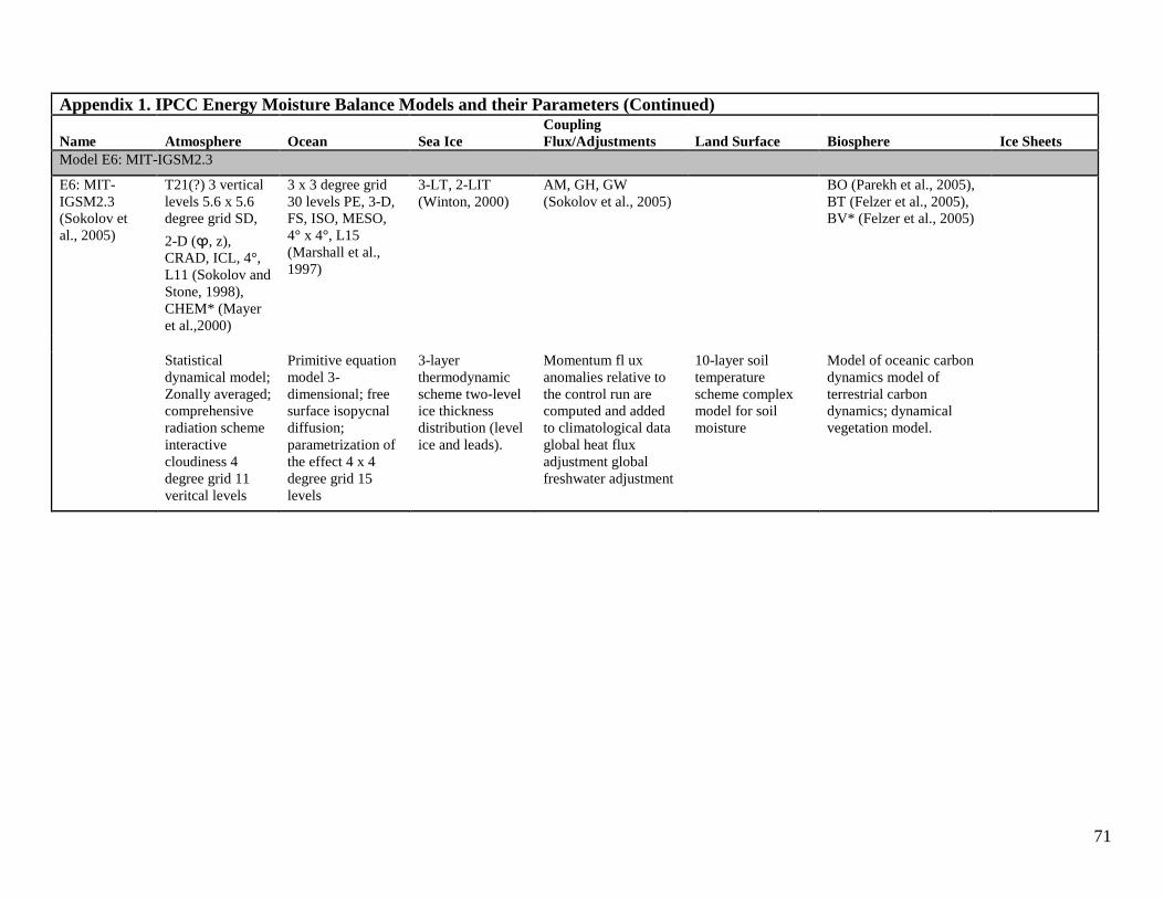
71

Appendix 1. IPCC Energy Moisture Balance Models and their Parameters (Continued)

Name Atmosphere Ocean Sea Ice Coupling Flux/Adjustments Land Surface Biosphere Ice Sheets

Model E6: MIT-IGSM2.3

E6: MIT-IGSM2.3 (Sokolov et al., 2005)

T21(?) 3 vertical levels 5.6 x 5.6 degree grid SD,

2-D (ϕ, z), CRAD, ICL, 4°, L11 (Sokolov and Stone, 1998), CHEM* (Mayer et al.,2000)

3 x 3 degree grid 30 levels PE, 3-D, FS, ISO, MESO, 4° x 4°, L15 (Marshall et al., 1997)

3-LT, 2-LIT (Winton, 2000)

AM, GH, GW (Sokolov et al., 2005)

BO (Parekh et al., 2005), BT (Felzer et al., 2005), BV* (Felzer et al., 2005)

Statistical

dynamical model; Zonally averaged; comprehensive radiation scheme interactive cloudiness 4 degree grid 11 veritcal levels

Primitive equation model 3-dimensional; free surface isopycnal diffusion; parametrization of the effect 4 x 4 degree grid 15 levels

3-layer thermodynamic scheme two-level ice thickness distribution (level ice and leads).

Momentum fl ux anomalies relative to the control run are computed and added to climatological data global heat flux adjustment global freshwater adjustment

10-layer soil temperature scheme complex model for soil moisture

Model of oceanic carbon dynamics model of terrestrial carbon dynamics; dynamical vegetation model.

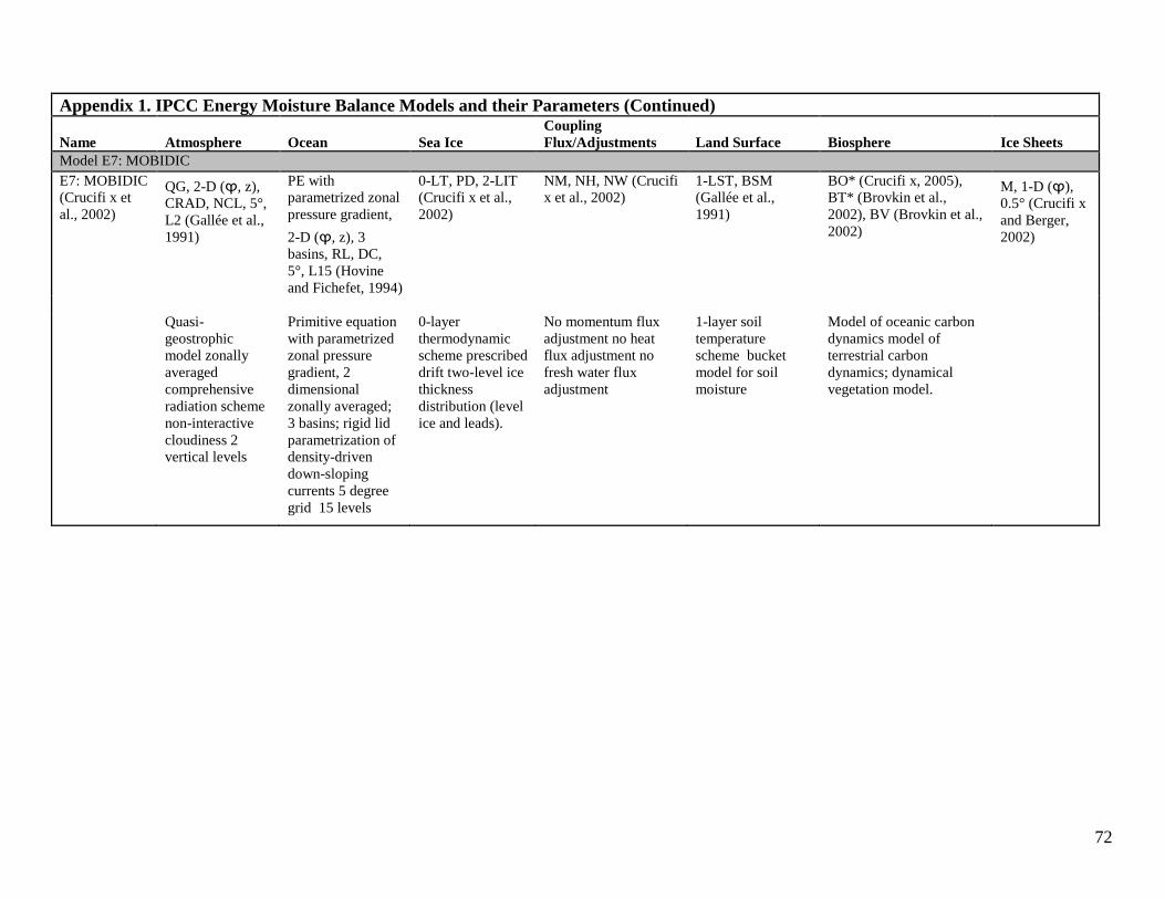
72

Appendix 1. IPCC Energy Moisture Balance Models and their Parameters (Continued)

Name Atmosphere Ocean Sea Ice Coupling Flux/Adjustments Land Surface Biosphere Ice Sheets

Model E7: MOBIDIC E7: MOBIDIC (Crucifi x et al., 2002)

QG, 2-D (ϕ, z), CRAD, NCL, 5°, L2 (Gallée et al., 1991)

PE with parametrized zonal pressure gradient,

2-D (ϕ, z), 3 basins, RL, DC, 5°, L15 (Hovine and Fichefet, 1994)

0-LT, PD, 2-LIT (Crucifi x et al., 2002)

NM, NH, NW (Crucifi x et al., 2002)

1-LST, BSM (Gallée et al., 1991)

BO* (Crucifi x, 2005), BT* (Brovkin et al., 2002), BV (Brovkin et al., 2002)

M, 1-D (ϕ), 0.5° (Crucifi x and Berger, 2002)

Quasi-

geostrophic model zonally averaged comprehensive radiation scheme non-interactive cloudiness 2 vertical levels

Primitive equation with parametrized zonal pressure gradient, 2 dimensional zonally averaged; 3 basins; rigid lid parametrization of density-driven down-sloping currents 5 degree grid 15 levels

0-layer thermodynamic scheme prescribed drift two-level ice thickness distribution (level ice and leads).

No momentum flux adjustment no heat flux adjustment no fresh water flux adjustment

1-layer soil temperature scheme bucket model for soil moisture

Model of oceanic carbon dynamics model of terrestrial carbon dynamics; dynamical vegetation model.

73

Appendix 1. IPCC Energy Moisture Balance Models and their Parameters (Continued)

Name Atmosphere Ocean Sea Ice Coupling Flux/Adjustments Land Surface Biosphere Ice Sheets

Model E8: UVIC E8: UVIC (Weaver et al., 2001)

DEMBM, 2-D

(ϕ, λ), NCL, 1.8° x 3.6° (Weaver et al., 2001)

PE, 3-D, RG, ISO, MESO, 1.8° x 3.6° (Weaver et al., 2001)

0-LT, R, 2-LIT (Weaver et al., 2001)

AM, NH, NW (Weaver et al., 2001)

1-LST, CSM, RIV (Meissner et al., 2003)

BO (Weaver et al., 2001), BT (Cox, 2001), BV (Cox, 2001)

M, 2-D (ϕ, λ), 1.8° x 3.6°* (Weaver et al., 2001)

Energy moisture balance model with some dynamics vertically averaged non-interactive cloudiness 1.8 x 3.6 degree grid

0-layer thermodynamic scheme viscous-plastic or elastic-viscous-plastic rheology two-level ice thickness distribution (level ice and leads).

Momentum fl ux anomalies relative to the control run are computed and added to climatological data no heat flux adjustment no fresh water flux adjustment

1-layer soil temperature scheme complex model for soil moisture river routing scheme

Model of oceanic carbon dynamics model of terrestrial carbon dynamics;

Note: a EMBM = energy-moisture balance model; DEMBM = energy-moisture balance model including some dynamics; SD = statistical-dynamical model; QG = quasi-

geostrophic model; 1-D (ϕ) = zonally and vertically averaged; 2-D(ϕ, λ) = vertically averaged; 2-D(ϕ, z) = zonally averaged; 3-D = three-dimensional; LRAD = linearized radiation scheme; CRAD = comprehensive radiation scheme; NCL = non-interactive cloudiness; ICL = interactive cloudiness; CHEM = chemistry module; horizontal and vertical resolutions: the horizontal resolution is expressed either as degrees latitude x longitude or as spectral truncation with a rough translation to degrees latitude x longitude;

the vertical resolution is expressed as ‘Lm’, where m is the number of vertical levels. b FG = frictional geostrophic model; PE = primitive equation model; 2-D (ϕ, z) = zonally averaged; 3-D = three-dimensional; RL = rigid lid; FS = free surface; ISO = isopycnal diffusion; MESO = parametrization of the effect of mesoscale eddies on tracer distribution; TCS = complex turbulence closure scheme; DC = parametrization of density-driven down-sloping currents; horizontal and resolutions: the horizontal resolution is expressed as degrees latitude x longitude; the vertical resolution is expressed as ‘Lm’, where m is the number of vertical levels.c n-LT = n-layer thermodynamic scheme; PD = prescribed drift; DOC = drift with oceanic currents; R = viscous-plastic or elastic-viscous-plastic rheology; 2-LIT = two-level ice thickness distribution (level ice and leads). Notes (continued):d PM = prescribed momentum fl ux; GM = global momentum fl ux adjustment; AM = momentum fl ux anomalies relative to the control run are computed and added to climatological data; NM = no momentum fl ux adjustment; GH = global heat fl ux adjustment; NH = no heat fl ux adjustment; GW = global freshwater fl ux

adjustment; RW = regional freshwater fl ux adjustment; NW = no freshwater fl ux adjustment.e NST = no explicit computation of soil temperature; n-LST = n-

layer soil temperature scheme; NSM = no moisture storage in soil; BSM = bucket model for soil moisture; CSM = complex model for soil

moisture; RIV = river routing scheme.f BO = model of oceanic carbon dynamics; BT = model of terrestrial carbon dynamics; BV = dynamical

vegetation model. g TM = thermomechanical model; M = mechanical model (isothermal); 1-D (ϕ) = vertically averaged with east-west parabolic profi le; 2-

D (ϕ, λ) = vertically averaged; 3-D = three-dimensional; horizontal and vertical resolutions: the horizontal resolution is expressed either as degrees latitude x longitude or kilometres x kilometres; the vertical resolution is expressed as ‘Lm’, where m is the number of vertical levels.

74