Climate Modeling: A Brief Exploration

Dr Hong YangDr Qin Leng

Collin Gagnon

April 9, 2014

Dr Brian Blaishttp://web.bryant.edu/~bblais

What is a Model?

What is a Model?

What is a Model?

Another advantage of explicit models is the feasibility of sensitivity analysis. One can

sweep a huge range of parameters over a vast range of possible scenarios to identify the

most salient uncertainties, regions of robustness, and important thresholds. I don't see

how to do that with an implicit mental model. It is important to note that in the policy

sphere (if not in particle physics) models do not obviate the need for judgment. However,

by revealing tradeoffs, uncertainties, and sensitivities, models can discipline the dialogue

about options and make unavoidable judgments more considered.

Can You Predict?

No sooner are these points granted than the next question inevitably arises: "But can you

predict?" For some reason, the moment you posit a model, prediction--as in a crystal ball

that can tell the future--is reflexively presumed to be your goal. Of course, prediction

might be a goal, and it might well be feasible, particularly if one admits statistical

prediction in which stationary distributions (of wealth or epidemic sizes, for instance) are

the regularities of interest. I'm sure that before Newton, people would have said "the

orbits of the planets will never be predicted." I don't see how macroscopic prediction--

pacem Heisenberg--can be definitively and eternally precluded.

Sixteen Reasons Other Than Prediction to Build Models

But, more to the point, I can quickly think of 16 reasons other than prediction (at least in

this bald sense) to build a model. In the space afforded, I cannot discuss all of these, and

some have been treated en passant above. But, off the top of my head, and in no

particular order, such modeling goals include:

1. Explain (very distinct from predict)

2. Guide data collection

3. Illuminate core dynamics

4. Suggest dynamical analogies

5. Discover new questions

6. Promote a scientific habit of mind

7. Bound (bracket) outcomes to plausible ranges

8. Illuminate core uncertainties.

9. Offer crisis options in near-real time

10. Demonstrate tradeoffs / suggest efficiencies

11. Challenge the robustness of prevailing theory through perturbations

12. Expose prevailing wisdom as incompatible with available data

13. Train practitioners

14. Discipline the policy dialogue

15. Educate the general public

16. Reveal the apparently simple (complex) to be complex (simple)

How many parameters?

y = mx+ b

data

2 parameters

How many parameters?

y = mx+ b

data

? parameters

How many parameters?

y = mx+ b

data

14 parameters

m1, b1

m5, b5t1

t4

Parameter Estimation and Uncertainty

y = mx+ b

2 parameters

Prediction

y = mx+ b

2 parameters

Should it surprise you to learn that this model predicts a significant temperature

increase over the next 100 years?

Two models

1.Evaporation Model With Isotope Data2.Oscillation Model with Temperature Data

Isotopes and Fractionation

•...are the same chemically (e.g. H2O, D2O)•...have different weight•...evaporate at different rates•...measured in modern and fossil leaves and sediments

Isotopes...

Model

(equator) (north pole)

E(✓)

✓ = 0 ✓ = 90

P (✓)E(✓) E(✓)

P (✓) P (✓)

H/L

Hp/LpHe/Le

Hprecip(✓) =H(✓)↵precip · P (✓)

L(✓) +H(✓)↵precip

Hevap(✓) =RSMOW · ↵evap · E(✓)

1 +RSMOW · ↵evap

Lprecip(✓) =L(✓) · P (✓)

L(✓) +H(✓)↵precip

Levap(✓) = E(✓)�Hevap =E(✓)

1 +RSMOW · ↵evap

dH

d✓= Hevap(✓)�Hprecip(✓)

dL

d✓= Levap(✓)� Lprecip(✓)

Rprecip = Hprecip/Lprecip

�precip =

✓Rprecip

RSMOW� 1

◆⇥ 1000

Given evaporation and precipitation profiles vs. latitude: E(θ) and P(θ)

Parcel moves from equator to pole, H and L isotope quantities in the vapor change

Fractionation processes modify the isotope quantities for evaporation and precipitation

δD values calculated from the precipitation

Evaporation and Precipitation

⌧E

⌧P

Latitude parameters

•Metasequoia and sediment samples were collected from known Middle Miocene deposits from across the Northern Hemisphere. •Several sample values used in this model have been previously collected and measured using relatively similar procedures and protocols.•Isotope-Ratio Mass-Spectrometer provides us with the ratio of deuterium to hydrogen (δ2H/1H) on the C-27, C-29, and C-31 n-alkanes.

Sample%Locations%Our&data&set&includes&8&Northern&Hemisphere&samples&(from&7&sites)&at&various&laFtudes&

Data

Evaporation

Precipitation

Dependence on Latitude

Exponential Model

Gaussian Model

Oscillation Model

Ecological Modelling 171 (2004) 433–450

Climate change: detection and attribution of trendsfrom long-term geologic data

Craig Loehle∗NCASI, 552 S. Washington Street #224, Naperville, IL 60540, USA

Received 6 August 2002; received in revised form 28 July 2003; accepted 13 August 2003

Abstract

Two questions about climate change remain open: detection and attribution. Detection of change for a complex phenomenonlike climate is far from simple, because of the necessary averaging and correcting of the various data sources. Given thatchange over some period is detected, how do we attribute that change to natural versus anthropogenic causes? Historical datamay provide key insights in these critical areas. If historical climate data exhibit regularities such as cycles, then these cyclesmay be considered to be the “normal” behavior of the system, in which case deviations from the “normal” pattern would beevidence for anthropogenic effects on climate. This study uses this approach to examine the global warming question. Two3000-year temperature series with minimal dating error were analyzed. A total of seven time-series models were fit to thetwo temperature series and to an average of the two series. None of these models used 20th Century data. In all cases, agood to excellent fit was obtained. Of the seven models, six show a warming trend over the 20th Century similar in timingand magnitude to the Northern Hemisphere instrumental series. One of the models passes right through the 20th Centurydata. These results suggest that 20th Century warming trends are plausibly a continuation of past climate patterns. Results arenot precise enough to solve the attribution problem by partitioning warming into natural versus human-induced components.However, anywhere from a major portion to all of the warming of the 20th Century could plausibly result from natural causesaccording to these results. Six of the models project a cooling trend (in the absence of other forcings) over the next 200 yearsof 0.2–1.4 ◦C.© 2003 Elsevier B.V. All rights reserved.

Keywords: Cyclic model; Climate history; Null model; Greenhouse gases; Solar forcing

1. Introduction

Two fundamental issues must be resolved in orderto address the climate change question: detection andattribution. Neither of these is simple in the case ofclimate change. Climate is a distributed and abstractproperty of weather, being neither directly measurablenor concrete. All climate records are necessarily con-structed from various instrumental records distributed

∗ Tel.: +1-630-579-1190; fax: +1-630-579-1195.E-mail address: cloehle@ncasi.org (C. Loehle).

across the globe. When proxy records (e.g. tree ringwidth, glacier extent), are used, the degree of abstrac-tion increases and the number of assumptions involvedin the analysis increases.For simple instrumental measures, detection of

change is simple. We can put a thermometer in apot of water and say that it has or has not changedits temperature compared to an hour ago. However,if the question is whether the behavior of a systemhas changed, we do not have such a simple detectionproblem. For example, if we wish to say whether thepattern of tornadoes is different this year compared

0304-3800/$ – see front matter © 2003 Elsevier B.V. All rights reserved.doi:10.1016/j.ecolmodel.2003.08.013

Oscillation Mathematics

C. Loehle / Ecological Modelling 171 (2004) 433–450 435

to know the mechanism in order to capture a periodicphenomenon. We can fit a curve to day length as afunction of the date at a locality without doing orbitalcalculations. Third, as an approximating function, asinusoidal model provides a starting point for moresophisticated models.I fit a cyclic model (Model 1) to the Sargasso data.

I estimated parameters by nonlinear minimization,based on a least-squares criterion using proceduresavailable in Mathematica. The model for temperaturedeviations from the temperature in 1975 is

Tt = a1× t + b1× cos[

π × (b2− t)

b3

]

+ c1× cos[

π × (c2− t)

c3

]

where T is temperature, t is time in years, a1 is thelinear cooling trend effect, b1 and b2 are cycle magni-tudes, and b3 and c3 are 1/2 cycle lengths. Additionalterms are added in later analyses. It uses a base yearof 2000 a.d. with years prior to this being negative(i.e. year 1975 is −25 ◦C) for ease of plotting. Threealternate models forms were tested.Prior studies (Bond et al., 2001; Broecker, 2001;

Campbell et al., 1998) have found a strong 1500years climate periodicity. Model 1 was thus fit witha 1500-year fixed cycle (parameter b3). A free-formfitting did not produce a better result. The best-fitparameter set for this model (Fig. 1A) isModel 1:

Tt = 0.000225× t + 0.354× cos[

π × (422.7− t)

750

]

+ 0.39× cos[

π × (37.9− t)

255.2

]

with a simple correlation of 0.41. All models dis-cussed are summarized in Table 1. The model hitsmajor peaks and valleys of the Sargasso data rea-sonably well. Of the peaks and troughs in modeland data, 67% line up, using a moving windowmeasure. These measures of fit are not outstanding,but are promising. Notably, the model and the databoth show a major peak during the Medieval WarmPeriod (800–1200 a.d.), which Broecker (2001) ar-gues was a globally warm interval, a conclusionsupported by deMenocal et al. (2000) and Soon and

Table 1Summary of cyclic models

Model Description Correlation Turnsstatistic(%)

1 Sargasso data: two-cycle,1500-year cycle fixed

0.41 67

2 Sargasso data: three-cycle,1500-year cycle fixed

0.52 76

3 Sargasso data: three-cycle 0.64 854 South Africa data: three-cycle 0.42 295 South Africa data: four-cycle 0.48 506 Two-series mean two-cycle 0.40 617 Two-series mean three-cycle 0.58 83

Baliunas (2003). Other studies also show the Me-dieval Warm Period (Little Climatic Optimum) inEurope (Lamb, 1965; Shindell et al., 2001), Green-land (Dahl-Jensen et al., 1998), Africa (deMenocalet al., 2000; Holmgren et al., 2001), North America(Campbell et al., 1998; Li et al., 2000; Petersen, 1994;Shabalova and Weber, 1999), South America (Iriondoet al., 1993; Villabala, 1994), and Asia (Hong et al.,2000; Liu et al., 1998). The Little Ice Age (1500–1850a.d.) is also captured by the model, with the beginningof this period of cooling coinciding with a model peakat 1500 a.d. followed by a long deep cold trough.The Maunder Minimum of 1700 a.d. (Shindell et al.,2001; Solankl et al., 2000) is located near the bottomof the last trough in the model (Fig. 1A). The LittleIce Age has been observed clearly by a variety ofmethods across the world (e.g. Campbell et al., 1998;D’Arrigo et al., 1998; Dahl-Jensen et al., 1998;deMenocal et al., 2000; Feng and Epstein, 1994;Fjellsa and Nordberg, 1996; Holmgren et al., 1999;Hong et al., 2000; Iriondo et al., 1993; Karlén et al.,1999; Kaser, 1999; Lamb, 1965; Li et al., 2000; Liuet al., 1998; Petersen, 1994; Shabalova and Weber,1999; Shindell et al., 2001; Villabala, 1994). Anothermeasure of model fit is the relation of the coefficientsto prior studies. The linear cooling trend (parametera1) of 0.23 ◦C/1000 years corresponds closely to acooling of about 0.25 ◦C/1000 years observed sincethe peak of the interglacial warm period 6000 to 8000BP (Beck, 1998; Dahl-Jensen et al., 1998; Feng andEpstein, 1994; Fischer et al., 1999; Pielou, 1993;Petit et al., 1999; Yu et al., 1998) and seen in priorclimate reconstructions (e.g. Crowley, 2000; Jones,1998; Mann et al., 1998, 1999; Overpeck et al., 1997).

Two Oscillations

436 C. Loehle / Ecological Modelling 171 (2004) 433–450

-1 .0

-0 .5

0 .0

0 .5

1 .0

1 .5

2 .0

2 .5

-1 5 0 0 -1 0 0 0 -5 0 0 0 5 0 0 1 0 0 0 1 5 0 0 2 0 0 0

Calendar Years

Tem

pera

ture

Dev

iatio

n ˚C

Little Ice Age

MedievalWarmPeriod

MedievalWarmPeriod

-1 .0

-0 .5

0 .0

0 .5

1 .0

1 .5

2 .0

2 .5

-1 5 0 0 -1 0 0 0 -5 0 0 0 5 0 0 1 0 0 0 1 5 0 0 2 0 0 0

Calendar Years

Tem

pera

ture

Dev

iatio

n ˚C

Little Ice Age

(A)

(B)

-1 .0

-0 .5

0 .0

0 .5

1 .0

1 .5

2 .0

2 .5

-1 5 0 0 -1 0 0 0 -5 0 0 0 5 0 0 1 0 0 0 1 5 0 0 2 0 0 0

Calendar Years

Tem

pera

ture

Dev

iatio

ns ˚C

MedievalWarmPeriod

Little Ice Age(C)

Fig. 1. Comparison of cyclic models (darker line) fit to the Sargasso SST data (from Keigwin, 1996). Temperatures as deviations from1975 values (◦C). The Medieval Warm Period of 800–1200 a.d. and the Little Ice Age of 1500–1850 a.d. (Broecker, 2001) are clearlyseen in both the model and data. (A) Model 1, (B) Model 2, (C) Model 3.

C. Loehle / Ecological Modelling 171 (2004) 433–450 435

to know the mechanism in order to capture a periodicphenomenon. We can fit a curve to day length as afunction of the date at a locality without doing orbitalcalculations. Third, as an approximating function, asinusoidal model provides a starting point for moresophisticated models.I fit a cyclic model (Model 1) to the Sargasso data.

I estimated parameters by nonlinear minimization,based on a least-squares criterion using proceduresavailable in Mathematica. The model for temperaturedeviations from the temperature in 1975 is

Tt = a1× t + b1× cos[

π × (b2− t)

b3

]

+ c1× cos[

π × (c2− t)

c3

]

where T is temperature, t is time in years, a1 is thelinear cooling trend effect, b1 and b2 are cycle magni-tudes, and b3 and c3 are 1/2 cycle lengths. Additionalterms are added in later analyses. It uses a base yearof 2000 a.d. with years prior to this being negative(i.e. year 1975 is −25 ◦C) for ease of plotting. Threealternate models forms were tested.Prior studies (Bond et al., 2001; Broecker, 2001;

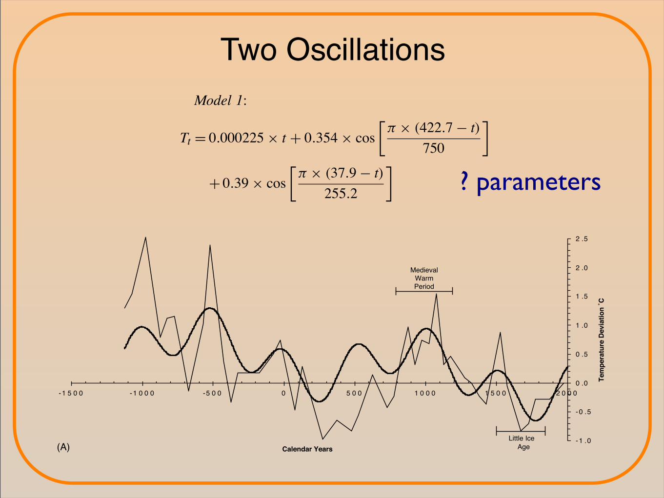
Campbell et al., 1998) have found a strong 1500years climate periodicity. Model 1 was thus fit witha 1500-year fixed cycle (parameter b3). A free-formfitting did not produce a better result. The best-fitparameter set for this model (Fig. 1A) isModel 1:

Tt = 0.000225× t + 0.354× cos[

π × (422.7− t)

750

]

+ 0.39× cos[

π × (37.9− t)

255.2

]

with a simple correlation of 0.41. All models dis-cussed are summarized in Table 1. The model hitsmajor peaks and valleys of the Sargasso data rea-sonably well. Of the peaks and troughs in modeland data, 67% line up, using a moving windowmeasure. These measures of fit are not outstanding,but are promising. Notably, the model and the databoth show a major peak during the Medieval WarmPeriod (800–1200 a.d.), which Broecker (2001) ar-gues was a globally warm interval, a conclusionsupported by deMenocal et al. (2000) and Soon and

Table 1Summary of cyclic models

Model Description Correlation Turnsstatistic(%)

1 Sargasso data: two-cycle,1500-year cycle fixed

0.41 67

2 Sargasso data: three-cycle,1500-year cycle fixed

0.52 76

3 Sargasso data: three-cycle 0.64 854 South Africa data: three-cycle 0.42 295 South Africa data: four-cycle 0.48 506 Two-series mean two-cycle 0.40 617 Two-series mean three-cycle 0.58 83

Baliunas (2003). Other studies also show the Me-dieval Warm Period (Little Climatic Optimum) inEurope (Lamb, 1965; Shindell et al., 2001), Green-land (Dahl-Jensen et al., 1998), Africa (deMenocalet al., 2000; Holmgren et al., 2001), North America(Campbell et al., 1998; Li et al., 2000; Petersen, 1994;Shabalova and Weber, 1999), South America (Iriondoet al., 1993; Villabala, 1994), and Asia (Hong et al.,2000; Liu et al., 1998). The Little Ice Age (1500–1850a.d.) is also captured by the model, with the beginningof this period of cooling coinciding with a model peakat 1500 a.d. followed by a long deep cold trough.The Maunder Minimum of 1700 a.d. (Shindell et al.,2001; Solankl et al., 2000) is located near the bottomof the last trough in the model (Fig. 1A). The LittleIce Age has been observed clearly by a variety ofmethods across the world (e.g. Campbell et al., 1998;D’Arrigo et al., 1998; Dahl-Jensen et al., 1998;deMenocal et al., 2000; Feng and Epstein, 1994;Fjellsa and Nordberg, 1996; Holmgren et al., 1999;Hong et al., 2000; Iriondo et al., 1993; Karlén et al.,1999; Kaser, 1999; Lamb, 1965; Li et al., 2000; Liuet al., 1998; Petersen, 1994; Shabalova and Weber,1999; Shindell et al., 2001; Villabala, 1994). Anothermeasure of model fit is the relation of the coefficientsto prior studies. The linear cooling trend (parametera1) of 0.23 ◦C/1000 years corresponds closely to acooling of about 0.25 ◦C/1000 years observed sincethe peak of the interglacial warm period 6000 to 8000BP (Beck, 1998; Dahl-Jensen et al., 1998; Feng andEpstein, 1994; Fischer et al., 1999; Pielou, 1993;Petit et al., 1999; Yu et al., 1998) and seen in priorclimate reconstructions (e.g. Crowley, 2000; Jones,1998; Mann et al., 1998, 1999; Overpeck et al., 1997).

Two Oscillations

436 C. Loehle / Ecological Modelling 171 (2004) 433–450

-1 .0

-0 .5

0 .0

0 .5

1 .0

1 .5

2 .0

2 .5

-1 5 0 0 -1 0 0 0 -5 0 0 0 5 0 0 1 0 0 0 1 5 0 0 2 0 0 0

Calendar Years

Tem

pera

ture

Dev

iatio

n ˚C

Little Ice Age

MedievalWarmPeriod

MedievalWarmPeriod

-1 .0

-0 .5

0 .0

0 .5

1 .0

1 .5

2 .0

2 .5

-1 5 0 0 -1 0 0 0 -5 0 0 0 5 0 0 1 0 0 0 1 5 0 0 2 0 0 0

Calendar Years

Tem

pera

ture

Dev

iatio

n ˚C

Little Ice Age

(A)

(B)

-1 .0

-0 .5

0 .0

0 .5

1 .0

1 .5

2 .0

2 .5

-1 5 0 0 -1 0 0 0 -5 0 0 0 5 0 0 1 0 0 0 1 5 0 0 2 0 0 0

Calendar Years

Tem

pera

ture

Dev

iatio

ns ˚C

MedievalWarmPeriod

Little Ice Age(C)

Fig. 1. Comparison of cyclic models (darker line) fit to the Sargasso SST data (from Keigwin, 1996). Temperatures as deviations from1975 values (◦C). The Medieval Warm Period of 800–1200 a.d. and the Little Ice Age of 1500–1850 a.d. (Broecker, 2001) are clearlyseen in both the model and data. (A) Model 1, (B) Model 2, (C) Model 3.

C. Loehle / Ecological Modelling 171 (2004) 433–450 435

to know the mechanism in order to capture a periodicphenomenon. We can fit a curve to day length as afunction of the date at a locality without doing orbitalcalculations. Third, as an approximating function, asinusoidal model provides a starting point for moresophisticated models.I fit a cyclic model (Model 1) to the Sargasso data.

I estimated parameters by nonlinear minimization,based on a least-squares criterion using proceduresavailable in Mathematica. The model for temperaturedeviations from the temperature in 1975 is

Tt = a1× t + b1× cos[

π × (b2− t)

b3

]

+ c1× cos[

π × (c2− t)

c3

]

where T is temperature, t is time in years, a1 is thelinear cooling trend effect, b1 and b2 are cycle magni-tudes, and b3 and c3 are 1/2 cycle lengths. Additionalterms are added in later analyses. It uses a base yearof 2000 a.d. with years prior to this being negative(i.e. year 1975 is −25 ◦C) for ease of plotting. Threealternate models forms were tested.Prior studies (Bond et al., 2001; Broecker, 2001;

Campbell et al., 1998) have found a strong 1500years climate periodicity. Model 1 was thus fit witha 1500-year fixed cycle (parameter b3). A free-formfitting did not produce a better result. The best-fitparameter set for this model (Fig. 1A) isModel 1:

Tt = 0.000225× t + 0.354× cos[

π × (422.7− t)

750

]

+ 0.39× cos[

π × (37.9− t)

255.2

]

with a simple correlation of 0.41. All models dis-cussed are summarized in Table 1. The model hitsmajor peaks and valleys of the Sargasso data rea-sonably well. Of the peaks and troughs in modeland data, 67% line up, using a moving windowmeasure. These measures of fit are not outstanding,but are promising. Notably, the model and the databoth show a major peak during the Medieval WarmPeriod (800–1200 a.d.), which Broecker (2001) ar-gues was a globally warm interval, a conclusionsupported by deMenocal et al. (2000) and Soon and

Table 1Summary of cyclic models

Model Description Correlation Turnsstatistic(%)

1 Sargasso data: two-cycle,1500-year cycle fixed

0.41 67

2 Sargasso data: three-cycle,1500-year cycle fixed

0.52 76

3 Sargasso data: three-cycle 0.64 854 South Africa data: three-cycle 0.42 295 South Africa data: four-cycle 0.48 506 Two-series mean two-cycle 0.40 617 Two-series mean three-cycle 0.58 83

Baliunas (2003). Other studies also show the Me-dieval Warm Period (Little Climatic Optimum) inEurope (Lamb, 1965; Shindell et al., 2001), Green-land (Dahl-Jensen et al., 1998), Africa (deMenocalet al., 2000; Holmgren et al., 2001), North America(Campbell et al., 1998; Li et al., 2000; Petersen, 1994;Shabalova and Weber, 1999), South America (Iriondoet al., 1993; Villabala, 1994), and Asia (Hong et al.,2000; Liu et al., 1998). The Little Ice Age (1500–1850a.d.) is also captured by the model, with the beginningof this period of cooling coinciding with a model peakat 1500 a.d. followed by a long deep cold trough.The Maunder Minimum of 1700 a.d. (Shindell et al.,2001; Solankl et al., 2000) is located near the bottomof the last trough in the model (Fig. 1A). The LittleIce Age has been observed clearly by a variety ofmethods across the world (e.g. Campbell et al., 1998;D’Arrigo et al., 1998; Dahl-Jensen et al., 1998;deMenocal et al., 2000; Feng and Epstein, 1994;Fjellsa and Nordberg, 1996; Holmgren et al., 1999;Hong et al., 2000; Iriondo et al., 1993; Karlén et al.,1999; Kaser, 1999; Lamb, 1965; Li et al., 2000; Liuet al., 1998; Petersen, 1994; Shabalova and Weber,1999; Shindell et al., 2001; Villabala, 1994). Anothermeasure of model fit is the relation of the coefficientsto prior studies. The linear cooling trend (parametera1) of 0.23 ◦C/1000 years corresponds closely to acooling of about 0.25 ◦C/1000 years observed sincethe peak of the interglacial warm period 6000 to 8000BP (Beck, 1998; Dahl-Jensen et al., 1998; Feng andEpstein, 1994; Fischer et al., 1999; Pielou, 1993;Petit et al., 1999; Yu et al., 1998) and seen in priorclimate reconstructions (e.g. Crowley, 2000; Jones,1998; Mann et al., 1998, 1999; Overpeck et al., 1997).

? parameters

Three Oscillations

C. Loehle / Ecological Modelling 171 (2004) 433–450 437

The 511-year cycle corresponds to the 500-year cyclefound in ice cores and other series (e.g. Li et al.,1997; Magny, 1993; Mayewski et al., 1997). Model1 does not show a 210-year cycle as used by Damonand Jirikowic (1992a,b). Forcing a 210-year cycle toreplace the 511-year cycle produced a very poor fit.The 11-year solar cycle was found by Damon andJirikowic to have a very small influence and was notused here. Data resolution does not permit estimationof such a short cycle in any case.Two models were tried with a linear term plus three

cyclic terms. In the first (Model 2), the 1500-year fixedcycle was kept for comparison.Model 2:

Tt = 0.000206× t + 0.34× cos[

π × (401.0− t)

750

]

+ 0.38× cos[

π × (44.7− t)

255.9

]

+ 0.374× cos[

π × (78.7− t)

510.3

]

The fitting produced a model with 1500, 1021, and512-year cycles, and a linear cooling of 0.21 ◦C/1000years (Fig. 1B). The simple correlation of 0.52 showsimproved fit. The moving window turns comparisongives a 76% match, which is also an improvement.Model 3 was fit without any constraints.Model 3:

Tt = 0.000186× t + 0.50× cos[

π × (1089.0− t)

973.3

]

+ 0.39× cos[

π × (235.3− t)

−115.1

]

+ 0.383× cos[

π × (42.0− t)

521.8

]

The fitting found a linear cooling of 0.19 ◦C/1000years and cycles of 1947, 1044, and 230 years. Thelatter cycle is very close to the 210-year cycle used byDamon and Jirikowic (1992a,b). The simple correla-tion is 0.64 (0.68 if we drop the single point at year525 b.c. as anomalous). Of the peaks and troughs, 85%matched using the moving window analysis. Model 3is thus considered the best-fit model overall. It is alsothe most assumption-free model.

The three models show certain robust features. Allthree show the Medieval Warm Period and the Lit-tle Ice Age (discussed for Model 1). The Jones et al.(1999) northern hemisphere reconstruction (in devia-tions from the 1950 mean), is one of the best seriesdemonstrating the warming of the latter part of the20th Century. It is compared here to the three fittedmodels (Fig. 2). Note that because of data resolutionlimitations, the fitting procedure could not estimate cy-cles shorter than 100 years, and thus models and datain Fig. 2 differ somewhat in resolution. Furthermore,the Jones hemisphere-scale data and the Sargasso SSTdata should not be expected to respond in magnitudeto a given warming or cooling exactly the same. Thuswe are looking for overall shape and trend similarities,rather than point by point correspondence. Fine scaledetails of the Jones data are not reproducible by themodels, but century long trends predicted by the mod-els should be comparable to the trends in the data. Allthree models show a warming trend of the same mag-nitude as that in the historical record over the past 150years. Model 1 passes right through the average trendof the historical data (Fig. 2A). All three models are onthe proper scale (not too high or too low by any largeamount). It is notable that these results were obtainedwithout using any data from the 20th Century duringparameter estimation. In previous studies, Damon andJirikowic (1992a,b) and Broecker (1975) identified theGleissberg≈88-year cycle as important. Since this cy-cle has a period too short to be fit with this data set,it was added directly to Model 3 to obtain Model 3a(Fig. 2D) for comparison. In all cases, model resultsthat follow are presented both with and without theGleissberg cycle, for comparative purposes. Based onDamon and Jirikowic (1992a,b) this cycle was givena fixed minimum in 1810 and a modest amplitude of0.2 ◦C. By adding the Gleissberg solar cycle, quali-tative features of 20th Century climate are captured(Fig. 2D) and the fit from 1910 on is remarkable. Themodel in fact passes through 0 ◦C deviations exactly in1975, the base year for calculating temperature devi-ations in the original data. Model 3a predicts a warm-ing of 1.1 ◦C over the 20th Century, versus 0.78 ◦C forthe northern hemisphere data.It is not possible from these models to draw any

conclusions about the fine-scale details of 20th Cen-tury climate, since short cycles of solar activity, vol-canic activity, land-cover change, and earth-system

436 C. Loehle / Ecological Modelling 171 (2004) 433–450

-1 .0

-0 .5

0 .0

0 .5

1 .0

1 .5

2 .0

2 .5

-1 5 0 0 -1 0 0 0 -5 0 0 0 5 0 0 1 0 0 0 1 5 0 0 2 0 0 0

Calendar Years

Tem

pera

ture

Dev

iatio

n ˚C

Little Ice Age

MedievalWarmPeriod

MedievalWarmPeriod

-1 .0

-0 .5

0 .0

0 .5

1 .0

1 .5

2 .0

2 .5

-1 5 0 0 -1 0 0 0 -5 0 0 0 5 0 0 1 0 0 0 1 5 0 0 2 0 0 0

Calendar Years

Tem

pera

ture

Dev

iatio

n ˚C

Little Ice Age

(A)

(B)

-1 .0

-0 .5

0 .0

0 .5

1 .0

1 .5

2 .0

2 .5

-1 5 0 0 -1 0 0 0 -5 0 0 0 5 0 0 1 0 0 0 1 5 0 0 2 0 0 0

Calendar Years

Tem

pera

ture

Dev

iatio

ns ˚C

MedievalWarmPeriod

Little Ice Age(C)

Fig. 1. Comparison of cyclic models (darker line) fit to the Sargasso SST data (from Keigwin, 1996). Temperatures as deviations from1975 values (◦C). The Medieval Warm Period of 800–1200 a.d. and the Little Ice Age of 1500–1850 a.d. (Broecker, 2001) are clearlyseen in both the model and data. (A) Model 1, (B) Model 2, (C) Model 3.

? parameters

Prediction

C. Loehle / Ecological Modelling 171 (2004) 433–450 439

oscillations (e.g. ENSO) are not included. However,looking at decadal to century trends, the three mod-els based on the Sargasso data suggest that warmingduring the 20th Century is plausibly a continuationof historical trends. The variability between the mod-els means that a precise estimate of how much of thewarming is natural versus anthropogenic cannot bemade.If the models properly capture the periodicities and

trends of the last 3000 years, they are likely validfor extrapolation over a 200-year horizon. The modelscan thus be used to make forecasts in the absence ofchanges in other forcings (Fig. 3). Models 1 and 2 pre-dict a fairly flat response with a modest cooling trendbeginning in 75 years. Model 3, the best-fit model forthe Sargasso data, projects a cooling trend that beginsalmost immediately and reaches a trough 0.7 ◦C coolerthan today by about 2125, compared to a cooling trendof 0.7 ◦C by 2150 projected by Damon and Jirikowic(1992a). Model 3a (Model 3 plus the Gleissberg cy-cle) shows a cooling beginning about 2012 and reach-ing a low 1.0 ◦C lower than today by 2145, coincidingclosely with the projection of Damon and Jirikowic(1992a). These projections would all clearly indicatean anthropogenic warming signal if temperatures con-tinue to rise over the next two decades.

-0.8

-0.6

-0.4

-0.2

0.0

0.2

0.4

0.6

0.8

2000 2050 2100 2150 2200

Calendar Years

Tem

pera

ture

Dev

iatio

n ˚C

model 1model 2model 3model 3a

Fig. 3. A 200-year projection of climate using the models fit to the Sargasso data. Temperatures as deviations from 1975 values (◦C).

To improve the estimate, a second long data se-ries (Holmgren et al., 1999, 2001) was evaluated. TheHolmgren data is derived from stalagmites in a cavein South Africa. Stalagmite color was found to be re-liably correlated with regional temperatures due to theeffect of temperature on the concentration of humicmaterials entering the ground water. Ten control pointswere used to estimate dates based on 230Th/234U ra-tios. Temperatures were reported as deviations fromthe 1961–1990 regional mean, which approximates the1975 zero-deviation used in the Sargasso study. In or-der to combine the two series, it is critical that bothseries have minimal dating error. Otherwise, the signalin the combined series will be obscured. I believe thatdating error is indeed minimal in the two series usedhere, because the usual sources of such error (sedimentmixing, 14C calibration errors, etc.) are largely absentbecause of the unique depositional environments ofthe two sites and the careful dating procedures used.Most other long-term records have large dating errors,are based on tree rings, which are not reliable for thispurpose (Broecker, 2001), or are too short for estimat-ing long-term cyclic components of climate (Fig. 3).Models with three and four cycles were fit to the

cave data. The three-cycle model (Model 4, Fig. 4A)fits reasonably well, with a correlation of 0.42.

Should it surprise you to learn that this model predicts a significant temperature decrease over the next 100 years?

Uncertainties

Period of Oscillation (years)

Period of Oscillation (years)

Uncertainties

Uncertainties in the period of

oscillations lead to uncertainties in the

pre/postdictions

Period of Oscillation (years)

Final ThoughtsSignificance&of&the&‘pause’&since&1998&

Under$condi?ons$of$anthropogenic$greenhouse$forcing:$•  Only$2%$of$climate$model$simula?ons$produce$trends$$$$$$$within$the$observa?onal$uncertainty$•  Modeled$pauses$longer$than$15$years$are$rare;$the$probability$of$a$

modeled$pause$exceeding$20$yrs$is$vanishing$small$

IPCC$AR5$

Extra

Modern values of and ⌧E ⌧P

and from an all-land model⌧E ⌧PModern (first run)

Miocene (first run) and from an all-land model⌧E ⌧P

Modern and from an all-ocean model⌧E ⌧P

Miocene and from an all-ocean model⌧E ⌧P

Modern and Climactic Variables81

DiscussionOur statistical analyses provide further insights into

how long-term climate signals may be registered in leaf tissues in the forms of stable isotopic compositions as well as elemental concentrations. The results include both predicted relationships as well as some surprises. An unexpected !nding is that there is no obvious re-lationship found between M. glyptostroboides leaf į13C values and any climate parameters. This is rather surprising given that among other factors, water avail-ability in particular is rather important in controlling 13C discrimination during photosynthesis (Warren et al., 2001), as indicated in previous studies using plant foliar (Hartman & Danin, 2010; Kloeppel et al., 1998) and tree ring (Loader et al., 2007) material. A recent global survey revealed strong relationship between plant į13C values and annual mean precipitation (AMP)

(Diefendorfa et al., 2010). We believe that it may be due to the unique water availability in these botanical gardens and university campuses where these culti-vated trees have been cared by supplementary arti!cial water (also see discussion below). On the other hand, we noticed that the carbon concentration is correlated with all four climate parameters with the strongest sup-port for a positive relationship with the annual mean precipitation (AMP) (Fig. 3C). To our knowledge, this is the !rst time when such an observation is made, and it may re"ect the particular growing habit of M. glyp-tostroboides that is largely dependent on large water supplies. It is known that the rapid growth of drought-intolerant M. glyptostroboides trees is heavily depen-dent on water availability (Vann, 2005). Both !eld ob-servations (Kuser, 1982) and greenhouse experiments (Jagels & Day, 2004; Jagels et al., 2003) demonstrated

Fig. 3 Correlations between isotope/elemental concentrations and climatic variables. — A: įD values against latitude, B: įD values against annual temperatures, C: bulk carbon against annual precipitation, D: bulk carbon against spring time temperatures, E: įD values against spring time tempera-tures, F: bulk nitrogen against spring time precipitation.

Stable isotope variations from cultivated Metasequoia trees in the United States (H. Yang et al.)

�D

81

DiscussionOur statistical analyses provide further insights into

how long-term climate signals may be registered in leaf tissues in the forms of stable isotopic compositions as well as elemental concentrations. The results include both predicted relationships as well as some surprises. An unexpected !nding is that there is no obvious re-lationship found between M. glyptostroboides leaf į13C values and any climate parameters. This is rather surprising given that among other factors, water avail-ability in particular is rather important in controlling 13C discrimination during photosynthesis (Warren et al., 2001), as indicated in previous studies using plant foliar (Hartman & Danin, 2010; Kloeppel et al., 1998) and tree ring (Loader et al., 2007) material. A recent global survey revealed strong relationship between plant į13C values and annual mean precipitation (AMP)

(Diefendorfa et al., 2010). We believe that it may be due to the unique water availability in these botanical gardens and university campuses where these culti-vated trees have been cared by supplementary arti!cial water (also see discussion below). On the other hand, we noticed that the carbon concentration is correlated with all four climate parameters with the strongest sup-port for a positive relationship with the annual mean precipitation (AMP) (Fig. 3C). To our knowledge, this is the !rst time when such an observation is made, and it may re"ect the particular growing habit of M. glyp-tostroboides that is largely dependent on large water supplies. It is known that the rapid growth of drought-intolerant M. glyptostroboides trees is heavily depen-dent on water availability (Vann, 2005). Both !eld ob-servations (Kuser, 1982) and greenhouse experiments (Jagels & Day, 2004; Jagels et al., 2003) demonstrated

Fig. 3 Correlations between isotope/elemental concentrations and climatic variables. — A: įD values against latitude, B: įD values against annual temperatures, C: bulk carbon against annual precipitation, D: bulk carbon against spring time temperatures, E: įD values against spring time tempera-tures, F: bulk nitrogen against spring time precipitation.

Stable isotope variations from cultivated Metasequoia trees in the United States (H. Yang et al.)

Yang, H., Blais, B.S., Leng, Q. 2011. Stable isotope variations from cultivated Metasequoia trees in the United States: A statistical approach to assess isotope signatures as climate signals. Jpn. J. His tor. Bot. 19 (1-2) pp 75-88.