NWS Science &Technology Infusion Climate Bulletin Supplement

34th NOAA Climate Diagnostics and Prediction Workshop Special Issue

Inside this issue:

1. The extratropical flow response to recurving western North Pacific tropical cyclones

H. M. Archambault, D. Keyser and L. F. Bosart ………… 1 2. Dominant modes of variability in the western U.S. coastal

cyclonic activity: Dynamical origins and impacts on the precipitation characteristics

Yi Deng ………… 5 3. Evaluation of 9 years of CPC long range precipitation fore-

casts in the northern Sierra Nevada of California Maury Roos ………… 11 4. The Pacific QDO as a natural predictor for the Great Salt

Lake elevation Robert R. Gillies and Shih-Yu Wang ………… 15

Climate Prediction S&T Digest

NOAA’s National Weather

Service

Office of Science and Technology 1325 East West Highway Silver Spring, MD 20910

Climate Prediction Center 5200 Auth Road Camp Springs, MD 20746

Monterey, CA

December 2009

NWS Science and Technology Infusion Climate Bulletin

http://www.nws.noaa.gov/ost/climate/STIP/index.htm

Science and Technology Infusion Climate Bulletin NOAA’s National Weather Service 34th NOAA Annual Climate Diagnostics and Prediction Workshop Monterey, CA, 26-30 October 2009

______________ Correspondence to: Heather M. Archambault, Department of Atmospheric and Environmental Sciences, University at Albany, State University of New York; E-mail: heathera@atmos.albany.edu

The Extratropical Flow Response to Recurving Western North Pacific Tropical Cyclones

Heather M. Archambault, Daniel Keyser and Lance F. Bosart Department of Atmospheric and Environmental Sciences, University at Albany, State University of New York

1. Introduction

Case studies of tropical cyclones that recurve and undergo extratropical transition (ET) over the western North Pacific (e.g., Harr and Dea 2009) reveal that recurving TCs can initiate or amplify Rossby wave trains along the North Pacific jet stream. The North Pacific basin is particularly favorable for Rossby wave train activity because of the near year-round occurrence of recurving western North Pacific TCs and the presence of an intense, longitudinally extensive extratropical jet stream (i.e., waveguide) during fall, winter, and spring. Understanding the factors that determine whether a high-amplitude Rossby wave train will be initiated or amplified by a recurving western North Pacific TC is a critical forecasting problem since such wave trains can persist on time scales of a week or more and can act as precursors to extreme weather events over North America.

The downstream response to a recurving western North Pacific TC is believed to depend on a variety of factors, including characteristics of the North Pacific jet stream and the presence of a preexisting upper-level trough or wave packet interacting with the TC. Since the latitude at which a TC recurves is strongly modulated by the strength and latitudinal position of the extratropical jet stream (e.g., Burroughs and Brand 1973), TCs recurving at different latitudes might be expected to produce different downstream responses because of different ambient jet stream characteristics. In this study, the Rossby wave train responses to western North Pacific TCs that recurve at different latitudes are compared using compositing. The compositing technique is detailed in section 2, key results are presented in section 3, and concluding remarks are contained in section 4.

2. Compositing technique

Western North Pacific recurving TCs are selected for compositing from the 413 TC recurvature episodes identified in a 30-year (1979–2008) best-track dataset constructed by the Regional Specialized Meteorological Center Tokyo-Typhoon Center. Based on Fig. 1, which shows the distribution of western North Pacific TC recurvature latitude, the three 5° latitude bands with the most TC recurvatures (15°–20°N, 20°–25°N, and 25°–30°N) are chosen as bins for compositing. To select for like recurving TC cases, additional criteria for compositing are: (i) the TC must be at typhoon strength at the time of recurvature, (ii) the TC must recurve between 125° and 145°E, (iii) the TC must obtain extratropical status at some point in its lifetime (i.e., complete ET), and (iv) the TC must not recurve within 10 days of another TC in the same composite bin. Using these criteria, 24 TCs are obtained for the 15°–20°N bin, 39 for the 20°–25°N

Fig. 1. Histogram of recurvature latitude for all 1979–2008 recurving western North Pacific TCs (n=413).

SCIENCE AND TECHNOLOGY INFUSION CLIMATE BULLETIN

2

bin, and 32 for the 25°–30°N bin. So that each composite bin contains the same number of members, 24 TCs are randomly selected for compositing from the TCs contained in the 20°–25°N and 25°–30°N bins.

The compositing procedure is “TC-recurvature-point centered” (i.e., individual member grids are spatially shifted so that the composite members are centered on the centroid of the TC recurvature points). Composite analyses are created using the 2.5° NCEP-NCAR reanalysis dataset (Kalnay et al. 1996; Kistler et al. 2001), and are shown for Day –1, Day +1, and Day +4 relative to the day of TC recurvature (Day 0). Composite 300-hPa meridional wind anomalies are calculated based on a 1979–2008 climatology, and statistical significance is assessed using a two-sided Student’s t test.

3. Results

Figures 2–4 illustrate distinct differences between the composite extratropical flow pattern surrounding TC recurvatures within the 15°–20°N, 20°–25°N, and 25°–30°N bands, hereafter lower-latitude (LL), middle-latitude (ML), and higher-latitude (HL) recurving TCs, respectively. One day prior to TC recurvature (Day –1; Fig. 2), an upper-tropospheric trough–ridge–trough pattern (i.e., a Rossby wave train) is apparent over southeastern Asia and the western North Pacific poleward of the TC in the LL composite, whereas no such pattern can be discerned in the ML and HL composites. Additionally, a region of strong upper-tropospheric winds (i.e., at least 65-kt winds) embedded in the western North Pacific jet stream is more expansive and extends farther equatorward in the LL composite than in the ML and HL composites.

Two days later, at Day +1 (Fig. 3), the amplitude and wavelength of the wave train in the LL composite has increased, and the wave train now extends across most of the North Pacific. At this time in the LL composite, southerly upper-tropospheric winds associated with the recurving TC have merged with those associated with a trough embedded in the wave train. A similar wave Fig. 3. Same as in Fig. 2, except for Day +1.

Fig. 2. Day –1 analyses for the 25°–30°N, 20°–25°N, and 15°–20°N composite bins (top, middle, and bottom panels, respectively). Analyses show 925−850-hPa layer-averaged relative vorticity (red contours, every 1 × 10−5 s−1, starting at 2 × 10−5 s−1), 300-hPa meridional wind anomaly (shaded in m s−1 according to the color bar, with black closed contours denoting statistical significance at the 95% level), 300-hPa potential vorticity (blue, every 1 PVU), and 300-hPa wind (barbs, >10 m s−1 only). Composite locations of the recurving TC are denoted with the “T” symbol.

ARCHAMBAULT ET AL.

3

train has also emerged in the ML composite over the western and central North Pacific, although the southerly winds on the leading edge of the wave are weaker and the wavelength of the wave train is slightly shorter. In contrast to the other two composites, a wave train is absent from the HL composite: only a ridge has amplified along the western North Pacific jet stream as the recurving TC moves poleward. In all three composites, the maximum wind speed of the western North Pacific jet stream increases between Day –1 and Day +1, from 90 kt to 105 kt, 70 kt to 95 kt, and 65 kt to 70 kt for the LL, ML, and HL composites, respectively.

By Day +4 (Fig. 4), the wave trains in the LL and ML composites have advanced downstream, yielding a ridge near the western North American coast and trough over the U.S. Great Basin. Accompanying ridge amplification along the western North American coast is warm air advection over western Canada and southern Alaska (not shown) in association with a Gulf of Alaska surface low (Fig. 4). The HL composite does not indicate a pronounced ridge–trough couplet over the eastern North Pacific and western North America: instead, only a weak trough over the western U.S. is evident within a relatively low-amplitude, short-wavelength wave train.

To examine whether recurving TCs contained in the LL, ML, and HL composites are favored at particular times of the year, the monthly frequency of recurving TCs is plotted in Fig. 5 for the three composite bins and the overall (1979–2009) recurving TC climatology. This figure reveals that recurving TCs contained in each of the composite bins tend to be favored at different times of the year: The HL recurving TCs occur near the climatological peak in recurving TC activity (September), the ML recurving TCs tend to occur slightly later in the season (October), and the LL recurving TCs tend to occur even later, as well as substantially earlier, in the season (November and May, respectively).

4. Concluding remarks

The results of the composite analysis suggest that LL and ML recurving TCs over the western North Pacific tend to induce or amplify Rossby wave trains that are characterized by higher amplitudes and longer wavelengths than HL recurving TCs. The LL and ML recurving TCs tend to favor the amplification of a ridge along the western North American coast and a downstream trough over the U.S. Great Basin

Fig. 4. Same as in Fig. 2, except for Day +4. Composite locations of key surface lows are denoted with an “L” symbol.

Fig. 5. Monthly frequency of recurving western North Pacific TCs for the three composite bins (n=24) and for the 1979–2008 climatology (n=413).

SCIENCE AND TECHNOLOGY INFUSION CLIMATE BULLETIN

4

approximately four days after TC recurvature. The composite analysis also suggests that LL recurving TCs may be more likely to be associated with a preexisting wave packet over eastern Asia and the western North Pacific than ML and HL recurving TCs.

The composite analysis illustrates that western North Pacific TCs that recurve closer to the equator tend to do so in the presence of a jet stream that is relatively strong and displaced equatorward, suggesting that TCs that recurve closer to the equator may be favored in late fall or in spring rather than in peak recurving TC season (i.e., late summer and early fall). A relationship between TC recurvature latitude and time of year is corroborated by the increased number of spring and late fall TCs in the composite bins as the latitude of the TC recurvature bin decreases.

In conclusion, the findings of this study suggest that western North Pacific TCs that recurve in late fall or in spring, when the North Pacific jet stream is relatively strong and displaced equatorward, may be more likely to induce or amplify a Rossby wave train that impacts North America than TCs that recurve in late summer or early fall when the North Pacific jet stream is relatively weak and displaced poleward. Future work will investigate the extent that forecast skill and uncertainty associated with the downstream extratropical response to a western North Pacific recurving TC depend upon the latitude at which the TC recurves.

References

Burroughs, L. D., and S. Brand, 1973: Speed of tropical storms and typhoons after recurvature in the western North Pacific Ocean. J. Appl. Meteor., 12, 452–458.

Harr, P. A., and J. M. Dea, 2009: Downstream development associated with the extratropical transition of tropical cyclones over the western North Pacific. Mon. Wea. Rev., 137, 1295–1319.

Kalnay, E., and Coauthors, 1996: The NCEP/NCAR 40-Year Reanalysis Project. Bull. Amer. Meteor. Soc., 77, 437–471.

Kistler, R., and Coauthors, 2001: The NCEP–NCAR 50-Year Reanalysis: Monthly means CD-ROM and documentation. Bull. Amer. Meteor. Soc., 82, 247–267.

Science and Technology Infusion Climate Bulletin NOAA’s National Weather Service 34th NOAA Annual Climate Diagnostics and Prediction Workshop Monterey, CA, 26-30 October 2009

______________ Correspondence to: Yi Deng, School of Earth and Atmospheric Sciences, Georgia Institute of Technology, 311 Ferst Drive, Atlanta, GA 30332-0340; E-mail: yi.deng@eas.gatech.edu

Dominant Modes of Variability in the Western U.S. Coastal Cyclonic Activity: Dynamical Origins and Impacts on the

Precipitation Characteristics Yi Deng

School of Earth and Atmospheric Sciences Georgia Institute of Technology, Atlanta, GA

1. Introduction

Coastal cyclones developing over the central and eastern North Pacific are responsible for majority of the winter precipitation in the western U.S. When approaching the land, these cyclones can bring hurricane-force winds and heavy precipitation to the coastal area causing flooding and mudslides in the Pacific Northwest and California (Ely et al. 1993; 1994). Moving further inland, they also directly contribute to or trigger significant snowfall events in the Sierra Nevada and Rockies, therefore partly control the depth of mountain snowpack that is crucial for the spring and summer water supply in the Southwest (Serreze et al. 1999). The characteristics of coastal cyclonic activity, including location, frequency and intensity, therefore have strong implications for natural hazards mitigation and water resource management in the western U.S. Past studies have examined the climatology of the winter cyclones focusing on either their spatial distributions or the variations of their occurrence frequency across various timescales (e.g., Sanders and Gyakum 1980; Parker et al. 1989; Sinclair 1994; Lefevre and Nielsen-Gammon 1995; Serreze et al. 1997; Key and Chan 1999). Anomalous cyclone tracks are also recognized as an integral part of the extratropical response to El Niño that is characterized by wetter (drier) than normal conditions in the southern (northern) part of the western U.S. (Schonher and Nicholson 1989; Dettinger et al. 1998; Mo and Higgins 1998). Raphael and Cheung (1998) further pointed out that the dryness in California during the second half of 1980s was related to the diminished extent of coastal cyclonic activity near California. Despite the obvious significance, few studies, however, have attempted to give a systematic account of the variability in coastal cyclones. Here we made an initial effort to quantify the dominant modes of interannual variability in the western U.S. coastal cyclonic activity, explore their likely dynamical origins, and examine their impacts on both the total amount and intensity of the winter precipitation.

2. Data and Methods

The analysis was focused on 27 winters (DJF, 1979/80-2005/06). A cyclone tracking data based on the NCEP/NCAR reanalysis (Sinclair 1997) was used to identify coastal cyclones, which include those making actual landfalls and those bypassing the west coastline. For each coastal cyclone identified, the latitude, longitude, sea level pressure (SLP) and 1000mb geostrophic vorticity at the first track point that gets within 475km distance from the coastline were recorded for further analysis. Based on the latitude and vorticity of the coastal cyclones, a cyclonic activity function (CAF) was

Fig. 1. Locations of the coastal cyclones (“+”) and the histogram of their occurrence frequency across latitudes. (Myoung and Deng 2009)

SCIENCE AND TECHNOLOGY INFUSION CLIMATE BULLETIN

6

defined as the accumulated intensity of the coastal cyclones (e.g., sum of the vorticities of the coastal cyclones) in a winter in each 1º latitude interval from 26ºN to 52ºN.

Daily precipitation from the North American Regional Reanalysis (NARR) (Mesinger et al. 2006) was used in conjunction with the cyclone tracking data to estimate the contributions of the cyclone-induced precipitation to the winter total precipitation. In particular, the NARR daily accumulated precipitation was mapped onto the area under a cyclone’s precipitation sectors. Such an area is assumed to encompass 4/cosθ to the west, 8/cosθ° to the east and 7.5° to the north and south from the center of the cyclone, where θ is the latitude of the track point.

Empirical Orthogonal Function (EOF) analyses were applied to the CAF and the DJF-mean precipitation in 27 winters to identify the principal modes of interannual variability in the coastal cyclonic activity and in the precipitation, respectively. Linear correlation analysis was conducted to quantify the relationship between the CAF and the winter precipitation, and to seek the dynamical origins of the principal modes of CAF variability. Composite analysis based upon the extreme phases of the CAF variability was performed to quantify the impacts of anomalous cyclonic activity on both the frequency and intensity of the winter precipitation in the western U.S.

3. Results and discussions

All the coastal cyclones observed in the 27 winters (1979/80-2005/06) are indicated by “+” in Fig. 1. The histogram on the left shows the frequency distribution of the cyclones across different latitudes. The peak frequency is located in the northern Canada at 60°N. The southern and northern U.S. borders are another two regions with relatively high frequency of cyclone passages.

Figure 2 shows the four leading EOF modes of the CAF, i.e., EOFCAF1, EOFCAF2, EOFCAF3, and EOFCAF4. They account for 40.7%, 29.6%, 14.4% and 3.9% of the total interannual variance, respectively. EOFCAF1 is characterized by a monopole with peak amplitude between 40°N and 50°N (Fig.2a). EOFCAF2 (Fig. 2b) on the other hand has a dipole structure with opposite signs between the south (35°N-42°N) and north (45°N-52°N). It indicates that above-normal

Fig. 2. EOF1 (a), EOF2 (b), EOF3 (c), and EOF4 (d) of the cyclonic activity function (CAF). (Myoung and Deng 2009).

Fig. 3. Ratio of the cyclone-induced precipitation amount to the winter total precipitation in the western U.S. Contour interval is 0.05. (Myoung and Deng 2009)

DENG

7

cyclonic activity along the northwest coast of U.S. tends to be accompanied by below-normal activity along the southwest coast and vice versa. The third mode (Fig. 2c) shows opposite signs between 40°N-44°N and 26°N-38°N/47°N-52°N. Enhanced cyclonic activity over the central west coast of U.S. (40°N-44°N) is associated with weakened activity over the southern California and the US-Canada border and vice versa. The fourth mode (Fig. 2d) is characterized by a quadruple with peak amplitudes occurring north of 40°N.

The ratio of the precipitation induced by coastal cyclones to the winter total precipitation is displayed in Fig. 3. The value increases rapidly from about 0.45 in the inland region to about 0.65 in the coastal area with maximum values at the Pacific Northwest and southern California exceeding 0.7. On average, this ratio is above 0.6 at most coastal areas indicating that more than 60% of the total winter precipitation is associated with the Pacific cyclones. If only the cyclones that made actually landfalls were considered, this ratio dropped to about 0.3, showing the substantial contributions to precipitation by those bypassing cyclones.

To establish the linkage between the variability in coastal cyclonic activity and in precipitation, we first examined the leading EOFs of the DJF-mean precipitation in the western U.S. (Fig. 4). The first mode (EOFPRECIP1) is characterized by a monopole with maximum amplitude over the Pacific Northwest and northern California. The second mode (EOFPRECIP2) shows a dipole structure with opposite signs between the Pacific Northwest and California. Correlation analysis between the principal components (PCs) of the precipitation and those of the CAF reveals that EOFPRECIP1 and EOFPRECIP2 are significantly related to EOFCAF1 and EOFCAF2 at the 95% level, respectively (Table 1).

As the most pronounced interannual signal in the climate system, ENSO is expected to modulate the coastal cyclonic activity (Noel and Changnon 1998). This was demonstrated by a significant correlation of -0.38 between PCCAF2 and the NINO3.4 SSTA. Given also the linkage between PCCAF2 and PCPRECIP2, these results support the speculation that ENSO contributes to the dipole of precipitation variability by inducing changes in the preferred latitudes of cyclone tracks.

To identify other large-scale processes that are potentially coupled to the CAF variability, we computed the correlations between PCs of the CAF and indices of major teleconnection patterns that are active over the North Pacific in winter (Table 2). The positive PNA or negative TNH phase features a negative height

CC PCPRECIP1 PCPRECIP2 PCCAF1 0.50 -0.08 PCCAF2 -0.07 -0.53 PCCaF3 0.03 0.18 PCCAF4 0.11 -0.35

PCCAF1 PCCAF2 PCCAF3 PCCAF4 PNA 0.11 -0.31 0.36 0.13 TNH -0.17 0.59 -0.05 -0.06 AO -0.29 -0.11 -0.47 -0.21 NP 0.00 0.29 -0.50 -0.19

Fig. 4. EOF1 (a) and EOF2 (b) of the western U.S. winter precipitation. Contour interval is 0.02. (Myoung and Deng 2009)

Table 1. Correlation coefficients between PCs of the winter precipitation and PCs of the cyclonic activity function, CAF. Bolds are statistically significant at the 95% level. (Myoung and Deng 2009)

Table 2. Correlation coefficients of PCs of CAF with DJF-averaged indices of PNA, TNH, AO and NP. Bolds are statistically significant at the 95% level. (Myoung and Deng 2009)

SCIENCE AND TECHNOLOGY INFUSION CLIMATE BULLETIN

8

anomaly west of the North America and a strengthened, eastward-displaced subtropical jet (Mo and Livzey 1986; Livzey and Mo 1987). This anomalous circulation pattern tends to bring more storms to the lower latitudes. A relatively weaker correlation (-0.31) was found between PCCAF2 and PNA compared to the one (0.59) between PCCAF2 and TNH. This difference is actually consistent with the fact that PCCAF2 is strongly modulated by ENSO and TNH is a more direct response to ENSO compared to PNA (Mo and Livzey 1986; Livzey and Mo 1987). Both the Negative AO and NP phase correspond to a deepening of the Aleutian Low and a stronger subtropical jet, which tend to enhance the eastward propagation of synoptic-scale eddies over the eastern North Pacific and therefore increase cyclonic activity at the Pacific Northwest and northern California. The significant, negative correlations of PCCAF3 with AO (-0.47) and NP (-0.5) are consistent with this argument. On the one hand, the teleconnection patterns discussed above may dynamically drive key variability in the coastal cyclonic activity. On the other hand, it is equally important to recognize that anomalous cyclonic activity often provides positive feedback to a teleconnection pattern and plays a key role in initiating and maintaining large-scale flow anomalies characteristic of such teleconnection (Holopainen and Fortelius 1987; Mullen 1987; Lau and Nath 1991; Nakamura et al. 1997).

As the last step, we will try to quantify the impacts of the principal CAF variability on the characteristics of winter precipitation. Composite anomalies of various precipitation statistics were calculated based upon the extreme phases of the CAF EOFs. Fig. 5 shows the differences of these statistics between the composite PC+ and PC- winters which are defined respectively as the average over the 5 winters with the highest and lowest values of each CAF PC. The three statistics we examined are the number of rainy days per winter, the 95th percentile of the daily rate, and the probability of precipitation being heavy given a rainy day. The first statistics quantifies precipitation frequency and the latter two are measures of precipitation extremes.

For PC1 (Fig. 5a-c), drastic differences at 38°N-49°N (Fig. 5a) are associated with significant changes of the cyclonic activity at 40°N-50°N (Fig. 2a). The maximum difference exceeds 14 days (out of 90 days per winter) at certain locations, which is equivalent to 48% of the average number of rainy days per winter at those locations. Significant differences in the 95th percentile of the rain rate (Fig. 5b) are found along the northwest coast and in its adjacent inland regions. Changes are greater than 16 mm/day in part of the northern California and southern Oregon. The increased probability of heavy precipitation from PC1- to PC1+ winter is evident in the northwestern U.S. (Fig. 5c).

Fig. 5. Differences of the number of rainy days per winter (a), the 95th percentile of the daily rain rate (unit: mm/day) (b) and the probability of precipitation being heavy given a rainy day (c) between PC1+ and PC1- winters (See the text for definitions). (d)-(f) and (g)-(i) are the same as (a)-(c) except for the differences between PC2+ and PC2- winters and between PC3+ and PC3- winters, respectively. (Myoung and Deng 2009)

DENG

9

Fig. 5d, e and f (Fig. 5g, h and i) are the same as Fig. 5a, b and c but between PC2+ and PC2- winters (PC3+ and PC3- winters). For PC2, the most distinct feature is the dipole between the northwestern and the southwestern U.S. Negative phases of EOFCAF2 are clearly leading to increases not only in the winter total precipitation but also in the extremeness of precipitation in the Southwest. The differences found for PC3 (Fig. 5g, h and i) are also in agreement with the mean precipitation changes driven by EOFCAF3 (Fig. 2c). In the central California, while the increase in the number of rainy days (Fig. 5g) is equivalent to 20-45% of its mean values, changes exceeding 100% of the corresponding mean values are found in the 95th

percentile of

the daily rain rate.

4. Summary and conclusion

This study examined the interannual variability in the cyclonic activity along the U.S. Pacific coast and quantified its impact on the characteristics of winter precipitation in the western U.S. A cyclonic activity function (CAF) was derived from objectively-identified cyclone tracks in 27 winters (1979/80-2005/06). EOF1 of the CAF was found to be responsible for the EOF1 of the winter precipitation in the western U.S., which is a monopole mode centered over the Pacific Northwest and northern California. EOF2 of the CAF contributes significantly to the EOF2 of the precipitation, which indicates that above-normal precipitation in the Pacific Northwest and its immediate inland regions tends to be accompanied by below-normal precipitation in California and the Southwest and vice versa. While EOF2s of the CAF and precipitation are linked to the ENSO signal on interannual time scales, EOF3 of the CAF shows robust relationship with NP and hemispheric-scale variability such as AO. A composite analysis revealed that the leading CAF modes increase (reduce) the winter total precipitation by increasing (reducing) both the number of rainy days per winter and the extremeness of precipitation.

Recent modeling studies have shown that the Pacific storm track, where most west coast cyclones originate, tends to shift poleward in a warm climate (Hall et al. 1994; Yin 2005). It is of great socioeconomic significance for us to understand how this poleward shift projects onto the coastal cyclonic activity and how the changes in the cyclonic activity affects the trend and variability of winter precipitation in the western U.S. In this regard, an improved understanding of the large-scale circulation features that determine the characteristics of coastal cyclones and their sensitivity to increased atmospheric concentrations of greenhouse gases will certainly benefit the society from perspectives of both the natural hazards mitigation and the water resource management.

References

Dettinger, M. D., D. R. Cayan, H. F. Diaz, and D. M. Meko, 1998: North–south precipitation patterns in western North America on interannual-to-decadal timescales. J. Climate, 11, 3095–3111.

Ely, L. L., Y. Enzel, V. R. Baker, and D. R. Cayan, 1993: A 5000-Year record of extreme floods and climate change in the southwestern United States. Science, 262, 410-412.

——, ——, and D. R. Cayan, 1994: Anomalous North Pacific atmospheric circulation and large winter floods in the southwestern United States. J. Climate, 7, 977–987.

Hall, N. M. J., B. J. Hoskins, P. J. Valdes, and C. A. Senior, 1994: Storm tracks in a high resolution GCM with doubled carbon dioxide. Q. J. R. Meteorol. Soc., 120, 1209-1230.

Holopainen, E., and C. Fortelius, 1987: High-Frequency Transient Eddies and Blocking. J. Atmos. Sci., 44, 1632–1645.

Key J. R., and A. C. K. Chan, 1999: Multidecadal global and regional trends in 1000 mb and 500 mb cyclone frequencies. Geophys. Res. Lett., 26, 2053–2056.

Lau, N.C., and M.J. Nath, 1991: Variability of the Baroclinic and Barotropic Transient Eddy Forcing Associated with Monthly Changes in the Midlatitude Storm Tracks. J. Atmos. Sci., 48, 2589–2613.

Lefevre, R. J., and J. W. Nielsen-Gammon, 1995: An objective climatology of mobile troughs in the Northern Hemisphere. Tellus, 47A, 638–655.

SCIENCE AND TECHNOLOGY INFUSION CLIMATE BULLETIN

10

Livezey, R. E., and K. C. Mo, 1987: Tropical–extratropical teleconnections during the Northern Hemisphere winter. Part II: Relationships between monthly mean Northern Hemisphere circulation patterns and proxies for tropical convection. Mon. Wea. Rev., 115, 3115–3132.

Mo, K. C., and R. E. Livezey, 1986: Tropical–extratropical geopotential height teleconnections during the Northern Hemisphere winter. Mon. Wea. Rev., 114, 2488–2515.

——, and R. W. Higgins, 1998: Tropical influences on California precipitation. J. Climate, 11, 412–430. Mullen, S.L., 1987: Transient Eddy Forcing of Blocking Flows. J. Atmos. Sci., 44, 3–22. Myoung, B., and Y. Deng, 2009: Interannual Variability of the Cyclonic Activity along the U.S. Pacific

Coast: Influences on the Characteristics of Winter Precipitation in the Western United States. J. Climate, 22, 5732–5747.

Nakamura, H., M. Nakamura, and J.L. Anderson, 1997: The Role of High- and Low-Frequency Dynamics in Blocking Formation. Mon. Wea. Rev., 125, 2074–2093.

Noel, J., and D. Changnon, 1998: A Pilot Study Examining U.S. Winter Cyclone Frequency Patterns Associated with Three ENSO Parameters. J. Climate, 11, 2152–2159.

Parker S. S., J. T. Hawes, S. J. Colucci, and B. P. Hayden, 1989: Climatology of 500-mb cyclones and anticylones, 1950–85. Mon. Wea. Rev., 117, 558–570.

Raphael, M. N., and I. K. Cheung, 1998: North Pacific midlatitude cyclone characteristics and their effect upon winter precipitation during selected El Niño/Southern Oscillation events. Geophys. Res. Lett., 25, 527-530.

Sanders, F., and J.R. Gyakum, 1980: Synoptic-Dynamic Climatology of the “Bomb”. Mon. Wea. Rev., 108, 1589–1606.

Schonher, T., and S. E. Nicholson, 1989: The relationship between California rainfall and ENSO events. J. Climate, 2, 1258–1269.

Serreze M. C., F. Carse, R. G. Barry, and J. C. Rogers, 1997: Icelandic low cyclone activity: Climatological features, linkages with the NAO and relationships with recent changes in the Northern Hemisphere circulation. J. Climate, 10, 453–464.

——, M. P. Clark, R. L. Armstrong, D. A. McGinnis, and R. S. Pulwarty, 1999: Characteristics of the western U.S. snowpack from SNOTEL data. Water Resour. Res, 35, 2145–2160.

Sinclair, M. R., 1994: An objective cyclone climatology for the Southern Hemisphere. Mon. Wea. Rev., 122, 2239–2256.

——, 1997: Objective identification of cyclones and their circulation intensity, and climatology. Wea. Forecasting, 12, 591-608.

Yin, J. H., 2005: A consistent poleward shift of the storm tracks in simulations of 21st century climate. Geophys. Res. Lett, 32, L18701, doi:10.1029/2005GL023684.

Science and Technology Infusion Climate Bulletin NOAA’s National Weather Service 34rd NOAA Annual Climate Diagnostics and Prediction Workshop Monterey, CA, 26-30 October 2009

______________ Correspondence to: Maurice Roos, California Department of Water Resources, P.O. Box 219000, Sacramento, CA, 95821-9000; E-mail: mroos@water.ca.gov.

Evaluation of 9 years of CPC Long Range Precipitation Forecasts in the Northern Sierra Nevada of California

Maurice Roos California Department of Water Resources, Sacramento, CA

1. Background

The northern Sierra Nevada is the most important runoff region in California, furnishing much of the water for the two largest water projects in the State – the Federal Central Valley Project and the State Water Project – as well as most of the water for the Sacramento San Joaquin River Delta. Estimated precipitation accumulation during the water year is monitored using eight stations to represent the 15,700 square mile watershed of the four major rivers. See the map of Figure 1 for the locations of the eight stations. The nearly 70 year historical record for the eight station index is shown in Figure 2.

The Climate Prediction Center (CPC) of the National Weather Service (NWS) has been making long range weather forecasts for over a decade with 0.5 to 12.5 months lead time. For us, the ones with the greatest potential are for the winter season. On average, half the annual precipitation, whether rain or snow, occurs during the December through February period with three-fourths from November through March. See the pie chart in Figure 3. Reliable forecasts during the early part of the rainy season have the most value as many decisions on water delivery and crop planting are made at that time before the halfway point in the accumulation season. Shortly after the first of February, we add the snowpack measurements to the forecasting methodology and the reliability improves.

The CPC precipitation forecasts, as you know, use three categories: more than chance probability of being wetter or drier and no slant either way (equal chances). Once in a while they indicate a zone where the probability is such that the area will be near normal. Usually only small portions of the country will be marked as more likely to be wet or dry with the larger space being without a signal. Figure 4 is a recent precipitation forecast map showing how the information is presented. Most of the time a precipitation shift is fairly modest. The edges of the shaded areas are 33 percent and increase to 40 or 45 percent and rarely 50 percent chance of being in the wet or dry tercile.

Fig. 1. Location of the 8 northern Sierra index stations.

Fig. 2. Northern Sierra precipitation record by water year.

SCIENCE AND TECHNOLOGY INFUSION CLIMATE BULLETIN

12

2. Evaluation

We tested with the northern Sierra eight station record of monthly or 3 month period precipitation for 9 water years (WY) from 2000 through 2008 and the early portion of WY 2009. We looked at the 0.5 month lead for the 1 month outlook, the 1-3 month outlook, and the 4-6 month outlook. To do this we reviewed all the forecasts, noting which ones showed all or part of the northern Sierra watershed in one of the shaded forecast areas. We made a judgment on the strength of the shift away from normal. These ranged from a slight 1 percent shift to a shift of 9 percent. To test the skill we then checked whether the measured precipitation was more or less than median for the month or the 3 month period. The skill is when the actual precipitation was in the same direction as the forecast. If it went the opposite way, the forecast was wrong. For example, if the forecast was shaded toward a wetter condition, a hit would be when the actual precipitation was above median – the right direction. Slightly over half of the forecasts for the region showed EC, equal chances, that is no signal. The EC forecasts were not counted in computing skill.

Results are shown on the first table. They show some skill: the 0.5 month lead one month forecast Heidke skill was 24 percent, the 1-3 month forecast skill was 23 percent, and the 4-6 month skill was a surprising 18 percent. However, when we looked at just the 5 wet months, for November through March (Table 2), the skill fell apart with more wrong than right except for the 4-6 month which only had 5 cases, with an apparent 60 percent skill, but too small a sample. So what this shows is that the skill is in the drier months which don’t matter as much in water supply.

Another evaluation approach was to examine just the months where a stronger confidence of wetter or drier was indicated, using at least a 5 percent shift as a threshold. The sample size was small and this did not show any consistent skill either (Table 3).

Another way to look at forecast results is to see how often the actual precipitation fell in the upper or lower tercile and to use how often their direction, either wet or dry, was indicated in the forecasts. Skill could be shown if the actual precipitation during those calls were slightly higher than the 33 percent expected from chance. Again no skill was shown except marginally in the 4-6 month outlook (see Table 4).

In 2004, CPC started revising the 1 month forecast at the end of the month. This did help quite a bit with the skill for that period rising from 27 percent for the 0.5 month lead forecast to 61 percent for the end of month revised outlook. A major factor is that forecasters can look at end of month weather patterns then and so improvement would be expected.

Fig. 4. Sample of CPC seasonal precipitation forecast (Made in October 2009)

Fig. 3. Average monthly distribution of northern California precipitation.

ROOS

13

The last table, Table 5, shows the directional skill each year of the 9 years for each of the three forecasts evaluated. The two best years were 2006 and 2008. But results in the intervening 2007 year were poor, more wrong than right.

Table 3. Same as Table 1 but for the months where

a stronger confidence of wetter or drier condition was indicated. A stronger signal is one with a 5 percent of more shift.

Table 4. For observed northern Sierra precipitation falling in the upper or lower tercile, evaluation of CPC forecast according to the direction indication (wet or dry).

3. Use of the forecast

For early season water project operations, the owner agencies are quite conservative. They are always worried that the season could turn dry and they would be unable to deliver amounts promised early in the season. Therefore, initial estimates of delivery are based in water in storage in the reservoirs and the amount of runoff anticipated for dry future conditions, either at the 90 or 99 percent probability level. Figure 5 shows a sample of last season’s January 1 Sacramento River system runoff forecast and how it changed during the course of December. Project operators (and the bankers who make crop loans to farmers) want to be very sure the water is there before promising delivery. For the State Water Project (SWP), that means the first allocation, usually shortly after December 1, is often less than 50 percent supply. Last year, in WY 2009, it was only 10 percent, which eventually was raised to 40 percent in the third year of drought. At the same time estimates of delivery amounts to users to be expected with normal future weather conditions and 75 and 25 percent

Table 1. Evaluation of CPC 0.5 month lead northern

Sierra precipitation forecast (2000-2008). Table 2. Same as Table 1 but for 5 wet months and for November through March only.

Table 5. Evaluation of directional skill for 2000-2008.

SCIENCE AND TECHNOLOGY INFUSION CLIMATE BULLETIN

14

probabilities are provided to guide water users in planning for the ensuing year. Because of the emphasis on dependability, a potentially important forecast product would be for forecasters to be able, with high confidence, to rule out future dry conditions in the forecast period, a more difficult task.

Probability shifts in future precipitation can be worked into runoff forecasts. But, so far, there shifts are small on the order of 5 percent. Near median probabilities, a 5 percent shift translates into fairly small quantitative amounts. See Figures 6 and 7 for charts of the one month December and the 3 month December through February winter season historical probabilities of precipitation amounts. For example, a 5 percent shift near median conditions works out to only about 1 and ½ inches in the 3 month winter season precipitation. As long as the climatological dry end of the spectrum is possible, these small shifts don’t really change a seasonal runoff forecast much. Reliability, especially in precluding future dry conditions, will have to improve a lot before significant changes in water operations are likely. There is a better chance to make use of small shifts in outlook if an agency has a good backup supply, such as groundwater, to take up the slack if the forecast is wrong. Some of the water customers do have multiple water supplies and are able to use the probability products to guide their operational planning.

Fig. 6. Probability distribution of northern Sierra 8 station average precipitation for December (1922-1999).

Fig. 7. Same as Figure 6 except for December-February 3 month precipitation.

Some of the CPC long range skill in the past is due to strong El Nino years. There were no strong El Ninos in this 9 year period; the best was a moderate warming event in late 2002. We were coming out of a strong cold La Nina event in water year 2000 at the start of this evaluation and the first portion of 2008 also saw a significant La Nina. Skill did seem a little better in 2008 but since it was not good in 2000 I hesitate to think that the cool events help much in signaling northern California winter precipitation. But we need to keep trying.

Fig. 5. Sample of water supply forecast.

Sacramento River Unimpaired Runoff 2009 Water Year Forecast as of January 1, 2009

Science and Technology Infusion Climate Bulletin NOAA’s National Weather Service 34rd NOAA Annual Climate Diagnostics and Prediction Workshop Monterey, CA, 26-30 October 2009

______________ Correspondence to: Robert R. Gillies, Utah Climate Center/Department of Plants, Soils, and Climate, Utah State University, Logan, UT; E-mail: Robert.Gillies@usu.edu

The Pacific QDO as a Natural Predictor for the Great Salt Lake Elevation Robert R. Gillies and Shih-Yu Wang

Utah Climate Center/Department of Plants, Soils, and Climate Utah State University, Logan, UT

1. Introduction

The lake elevation of the Great Salt Lake (GSL), a large closed basin in the arid western United States, is characterized by a pronounced quasi-decadal oscillation (QDO) (Lall and Mann 1995). Wang et al. (2009a) found that the variation of the GSL elevation is very coherent with the QDO of sea surface temperature anomalies in the tropical central Pacific, known as the Pacific QDO (White and Liu 2008a, b). The Pacific QDO can be depicted by the SST anomalies in the NINO4 region (Allan 2000), denoted as ΔSST (NINO4). Fig. 1 illustrates the coherence between the GSL elevation and ΔSST (NINO4). However, such a coherence denies any direct association between the precipitation over the GSL watershed and the Pacific QDO because, in a given frequency, the precipitation variations always lead the GSL elevation variations. In other words, a direct link between the Pacific QDO and the precipitation source of the GSL is absent. What causes the GSL elevation to vary so coherently with ΔSST (NINO4) is therefore an intriguing question.

A pronounced quasi-decadal variability was observed in the Intermountain precipitation (cf. Fig.2c) as well as the GSL elevation (cf. Fig. 2b). Wang et al. (2009a) noted that the precipitation QDO in the Intermountain region consistently lags the Pacific QDO by a quarter-phase, i.e. 3 years after the peak of the warm-phase Pacific QDO occurs, an anomalous trough develops over the Gulf of Alaska and enhances the Intermountain precipitation. For the opposite, the cool-phase Pacific QDO, 3 years later an anomalous ridge forms in the same location and thus reduces the Intermountain precipitation. These findings lead to a hypothesis that the quasi-decadal coherence between ΔSST (NINO4) and the GSL elevation, as described in Fig. 1, reflects a sequential process that begins with the warm/cool phase of the Pacific QDO and ultimately affects the GSL elevation, through modulations of the quadrature amplitude modulation of the Pacific QDO on the intermountain precipitation. Here we examine this hypothesis by analyzing the meteorological and hydrological variables over the Great Basin.

2. Data

Gridded data used in the analysis included the Kaplan Extended SST (Kaplan et al. 1998), the U.K. Meteorological Office Hadley Centre's mean sea level pressure (HadSLP2; Allan and Ansell 2006), the NCEP/NCAR Global Reanalysis (Kalnay et al. 1996), and the gauge-based monthly precipitation (Legates and Willmott 1990), all of which were provided through the NOAA/OAR/ESRL PSD. Lake elevations of the GSL over the period of record were obtained from the United States Geological Survey (USGS). This

Fig. 1. Monthly GSL elevation (in feet; thick solid curve) and the Kaplan SST anomalies (°C) in the NINO4 region (160°E-150°W, 5°S-5°N) denoted as ΔSST(NINO4) (thick dashed curve), both were smoothed by a 6 year lowpass. The original time series of the GSL elevation and ΔSST (NINO4) are superimposed as gray thin curve and gray dashed curve, respectively.

SCIENCE AND TECHNOLOGY INFUSION CLIMATE BULLETIN

16

study used the post-1900 records of the GSL elevation measured at the Boat Harbor location southwest of the GSL.

3. Results

a. Statistics

Power spectrums of the monthly unfiltered ΔSST (NINO4), the GSL elevation, and the precipitation within the hydrological drainage basin of the GSL are given in Fig. 2a-c. Significant signals between 10 and 15 years are clearly visible. To examine the apparent association between ΔSST (NINO4) and the GSL elevation as noted in Fig. 1, we performed the multitaper method (MTM) of spectral coherence analysis (Mann and Park 1996) on both the GSL elevation and ΔSST (NINO4) over the period of record from 1900 to 2007. As shown in Fig. 2d, a high degree of coherence between the GSL elevation and ΔSST (NINO4) stands out in the 10-15 year frequency domain. The peak of this quasi-decadal coherence is significant at the 95% confidence level with a near 180° phase difference, supporting the out-of-phase relationship as was revealed in Fig. 1. The MTM coherence between ΔSST (NINO4) and the GSL elevation tendency (Fig. 2e) resembles Fig. 2d, except for a 90° phase difference in the 10-15 year frequency domain. These features were also observed in Fig. 2f, as the coherence between ΔSST (NINO4) and the precipitation is significant at the 99% confidence level. The compilation of results in Fig. 2 indicates that the Pacific QDO leads both the precipitation and the GSL elevation tendency by a quarter-phase. Because the GSL elevation tendency follows the precipitation which leads the GSL elevation by a another quarter-phase, the GSL elevation should lag ΔSST(NINO4) by a half-phase (180°) in this quasi-decadal time scale.

To substantiate the analysis given in Fig. 2, monthly time series of ΔSST (NINO4), the precipitation, and the GSL elevation were subsequently filtered using the Hamming-Windowed filter (Iacobucci and Noullez 2005) within the 10-15 year frequency band, the result of which is given in Fig. 3. The warm, cool, rising and falling transition phases of the QDO evolution in ΔSST (NINO4) are illustrated along with the precipitation and the GSL elevation. Immediately obvious is that all three time series exhibit clear quasi-

Fig. 2. The global wavelet power spectrum of monthly unfiltered (a) ΔSST (NINO4), (b) GSL elevation, and (c) precipitation within the GSL hydrological drainage basin from 1900 to 2007. (d), (e), (f) MTM coherence (solid curve) and phase (dotted curve) between ΔSST (NINO4) and the GSL elevation (d), the GSL elevation tendency (e), and Precipitation (f) respectively using three 2π tapers. Dotted lines in (a)-(c) indicate the 99% significance level determined by a red-noise (autoregressive lag 1) background spectrum. The dashed horizontal lines in (d)-(f) are the 90%, 95%, and 99% confidence limits for the coherence amplitude. Note that the phase lags of 180° and -180° are the same. The phase difference at 0.075 < f < 0.1 in (e) and (f) has ΔSST (NINO4) leading the GSL elevation tendency and the precipitation, respectively.

Fig. 2. Day –1 analyses for the 25°–30°N, 20°–25°N, and 15°–20°N composite bins (top, middle, and bottom panels, respectively). Analyses show 925−850-hPa layer-averaged relative vorticity (red contours, every 1 × 10−5 s−1, starting at 2 × 10−5 s−1), 300-hPa meridional wind anomaly (shaded in m s−1 according to the color bar, with black closed contours denoting statistical significance at the 95% level), 300-hPa potential vorticity (blue, every 1 PVU), and 300-hPa wind (barbs, >10 m s−1 only). Composite locations of the recurving TC are denoted with the “T” symbol.

GILLIES AND WANG

17

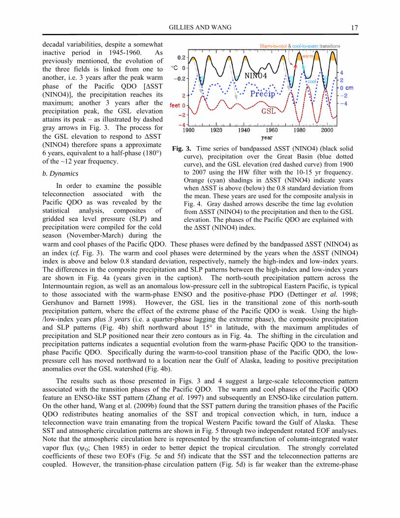
decadal variabilities, despite a somewhat inactive period in 1945-1960. As previously mentioned, the evolution of the three fields is linked from one to another, i.e. 3 years after the peak warm phase of the Pacific QDO [ΔSST (NINO4)], the precipitation reaches its maximum; another 3 years after the precipitation peak, the GSL elevation attains its peak – as illustrated by dashed gray arrows in Fig. 3. The process for the GSL elevation to respond to ΔSST (NINO4) therefore spans a approximate 6 years, equivalent to a half-phase (180°) of the ~12 year frequency.

b. Dynamics

In order to examine the possible teleconnection associated with the Pacific QDO as was revealed by the statistical analysis, composites of gridded sea level pressure (SLP) and precipitation were compiled for the cold season (November-March) during the warm and cool phases of the Pacific QDO. These phases were defined by the bandpassed ΔSST (NINO4) as an index (cf. Fig. 3). The warm and cool phases were determined by the years when the ΔSST (NINO4) index is above and below 0.8 standard deviation, respectively, namely the high-index and low-index years. The differences in the composite precipitation and SLP patterns between the high-index and low-index years are shown in Fig. 4a (years given in the caption). The north-south precipitation pattern across the Intermountain region, as well as an anomalous low-pressure cell in the subtropical Eastern Pacific, is typical to those associated with the warm-phase ENSO and the positive-phase PDO (Dettinger et al. 1998; Gershunov and Barnett 1998). However, the GSL lies in the transitional zone of this north-south precipitation pattern, where the effect of the extreme phase of the Pacific QDO is weak. Using the high-/low-index years plus 3 years (i.e. a quarter-phase lagging the extreme phase), the composite precipitation and SLP patterns (Fig. 4b) shift northward about 15° in latitude, with the maximum amplitudes of precipitation and SLP positioned near their zero contours as in Fig. 4a. The shifting in the circulation and precipitation patterns indicates a sequential evolution from the warm-phase Pacific QDO to the transition-phase Pacific QDO. Specifically during the warm-to-cool transition phase of the Pacific QDO, the low-pressure cell has moved northward to a location near the Gulf of Alaska, leading to positive precipitation anomalies over the GSL watershed (Fig. 4b).

The results such as those presented in Figs. 3 and 4 suggest a large-scale teleconnection pattern associated with the transition phases of the Pacific QDO. The warm and cool phases of the Pacific QDO feature an ENSO-like SST pattern (Zhang et al. 1997) and subsequently an ENSO-like circulation pattern. On the other hand, Wang et al. (2009b) found that the SST pattern during the transition phases of the Pacific QDO redistributes heating anomalies of the SST and tropical convection which, in turn, induce a teleconnection wave train emanating from the tropical Western Pacific toward the Gulf of Alaska. These SST and atmospheric circulation patterns are shown in Fig. 5 through two independent rotated EOF analyses. Note that the atmospheric circulation here is represented by the streamfunction of column-integrated water vapor flux (ψQ; Chen 1985) in order to better depict the tropical circulation. The strongly correlated coefficients of these two EOFs (Fig. 5e and 5f) indicate that the SST and the teleconnection patterns are coupled. However, the transition-phase circulation pattern (Fig. 5d) is far weaker than the extreme-phase

Fig. 3. Time series of bandpassed ΔSST (NINO4) (black solid curve), precipitation over the Great Basin (blue dotted curve), and the GSL elevation (red dashed curve) from 1900 to 2007 using the HW filter with the 10-15 yr frequency. Orange (cyan) shadings in ΔSST (NINO4) indicate years when ΔSST is above (below) the 0.8 standard deviation from the mean. These years are used for the composite analysis in Fig. 4. Gray dashed arrows describe the time lag evolution from ΔSST (NINO4) to the precipitation and then to the GSL elevation. The phases of the Pacific QDO are explained with the ΔSST (NINO4) index.

SCIENCE AND TECHNOLOGY INFUSION CLIMATE BULLETIN

18

one (Fig. 5c), corresponding to their associated SST patterns (Figs. 5a and 5b). Nonetheless, the teleconnection wave train during the transition-phase Pacific QDO is persistent and has direct impact on the Intermountain precipitation regime (Wang et al. 2009b). This forms the source of quasi-decadal signals recorded for the Intermountain precipitation as well as the GSL elevation.

Fig. 4. (a) Differences in precipitation (U. Delaware; shadings) and SLP (HadSLP2; contours) between composites of high-index years (1902-04, 1914-16, 1928-30, 1940-42, 1967-69, 1978-81, 1991-94, and 2003-05) and low-index years (1909-11, 1923, 1934-36, 1973-75, 1985-87, and 1997-2000) during the cold season (November of the previous year to March), based on the bandpassed ΔSST(NINO4) in Fig. 3. The contour interval of SLP is 0.5 hPa while precipitation below the 95% confidence level (t-test) is omitted. (b) Same as (a) but for the composites between high- and low-index years plus 3 years. Data are unfiltered. The GSL is indicated by a star. Significance level of SLP is not shown.

Fig. 5. (a) REOF 1 and (b) REOF 2 of the monthly Kaplan SST bandpassed by 10-15 year from 1948 to 2007. Contour interval is 0.1°C in (a) and 0.05°C in (b). (c) REOF 1 and (d) REOF 2 of the bandpassed column-integrated moisture flux streamfunction (ψQ). The normalized coefficients are shown in (e) and (f) as solid curves, with the coefficients of the bandpassed SST superimposed by shading; their correlation coefficients are shown in the upper left of (e) and (f). The teleconnection wave train is indicated by a red dashed arrow in panel (d).

4. Concluding remarks

Recurrent atmospheric circulation patterns develop over the Gulf of Alaska as a result of the teleconnection associated with the warm-to-cool and cool-to-warm transition phases of the Pacific QDO. These circulation patterns modulate transient synoptic activities over the western United States which, in turn,

GILLIES AND WANG

19

lead to a 3 year lag in both the precipitation and the hydrological cycle of the GSL watershed. The GSL elevation responds to such precipitation variations with a 3 year lag and therefore, it takes on average 6 years for the GSL elevation to respond to the warm/cool phases of the Pacific QDO. Such atmospheric and hydrological processes create a half-phase delay of the GSL elevation from the Pacific QDO, leading to their out-of-phase relationship as was shown in Fig. 1.

A proper monitoring of the status of the Pacific QDO evolution can therefore serve in part to predict the precipitation tendencies in the Great Basin and so, foretell the GSL elevation for future years. A conceptual model for such an application of the science was illustrated in Fig. 3.

References

Allan, R., 2000: ENSO and climatic variability in the last 150 years, El Niño and the Southern Oscillation: Multiscale Variability, Global and Regional Impacts, H. F. Diaz and V. Markgrav Ed., Cambridge Univ. Press, Cambridge, U.K, pp. 3–56.

Allan, R. J., and T. J. Ansell, 2006: A new globally-complete monthly historical gridded mean sea level pressure data set (HadSLP2): 1850-2004, J. Climate, 19, 5816-5842.

Chen, T.-C., 1985: Global water vapor flux and maintenance during FGGE. Mon. Wea. Rev., 113, 1801–1819.

Dettinger, M. D., D. R. Cayan, H. F. Diaz, and D. M. Meko, 1998: North–south precipitation patterns in western North America on interannual-to-decadal timescales. J. Climate, 11, 3095–3111.

Gershunov, A., and T. P. Barnett, 1998: Interdecadal modulation of ENSO teleconnections. Bull. Amer. Meteor. Soc., 79, 2715–2725.

Iacobucci, A. and A. Noullez, 2005: A frequency selective filter for short-length time series, Computational Economics, 25, 75-102.

Kalnay, E., and Co-Authors, 1996: The NCEP/NCAR 40-year reanalysis project, Bull. Amer. Meteor. Soc., 77, 437-470.

Kaplan, A., M. Cane, Y. Kushnir, A. Clement, M. Blumenthal, and B. Rajagopalan, 1998: Analyses of global sea surface temperature 1856-1991, J. Geophy. Res., 103, 567-589.

Lall, U., and M. Mann, 1995: The Great Salt Lake: A barometer of low-frequency climatic variability, Water Resour. Res., 31, 2503-2515.

Legates, D. R. and C. J. Willmott, 1990: Mean seasonal and spatial variability in gauge-corrected, global precipitation. Int. J. Climato., 10, 111-127.

Mann, M. E., Park. J., 1996: Greenhouse warming and changes in the seasonal cycle of temperature: Model versus observation, Geophy. Res. Lett., 23, 1111-1114.

Tourre, Y. M., B. Rajagopalan, Y. Kushnir, M. Barlow, and W. B. White, 2001: Patterns of coherent decadal and interdecadal climate signals in the Pacific Basin during the 20th Century. Geophys. Res. Lett., 28, 2069.

Wang, S.-Y., R. R. Gillies, J. Jin, and L. E. Hipps, 2009a: Coherence between the Great Salt Lake level and the Pacific quasi-decadal oscillation, J. Climate (in press), DOI: 10.1175/2009JCLI2979.1

____, ____, L. E. Hipps, and J. Jin, 2009b: A transition-phase teleconnection of the Pacific QDO, Climate Dynamics (http://cliserv.jql.usu.edu/paper/CD/pacific-qdo.pdf).

White W. B., and Z. Liu, 2008a: Non-linear alignment of El Niño to the 11-yr solar cycle, Geophys. Res. Lett., 35, L19607, doi:10.1029/2008GL034831.

____, and ____, 2008b: Resonant excitation of the quasi-decadal oscillation by the 11-year signal in the Sun’s irradiance, J. Geophys. Res., 113, C01002.

Zhang, Y., J. M. Wallace, and D. S. Battisti, 1997: ENSO-like interdecadal variability: 1900–93. J. Climate, 10, 1004–1020.