climate sensitivity: linear perspectives isaac held, jerusalem, jan 2009
DESCRIPTION
Climate Sensitivity: Linear Perspectives Isaac Held, Jerusalem, Jan 2009. 1. How can the response of such a complex system be “linear”?. Infrared radiation escaping to space - - 50km model under development at GFDL. 2. - PowerPoint PPT PresentationTRANSCRIPT

Climate Sensitivity: Linear Perspectives Isaac Held, Jerusalem, Jan 2009
1

Infrared radiation escaping to space -- 50km model under development at GFDL
How can the response of such a complex system be “linear”?
2

Response of global mean temperature to increasing CO2 seems simple, as one might expect from the simplest linear energy balance models
3

White areas => less than two thirds of the models agree on the sign of the change
Percentage change in precipitation by end of 21st century: PCMDI-AR4 archive
But we are not interested in global mean temperature, but rather things like the response in local precipitation
4
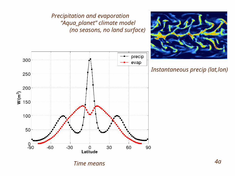
Precipitation and evaporation “Aqua_planet” climate model (no seasons, no land surface)
Instantaneous precip (lat,lon)
Time means 4a

Aqua planet (P – E) response to doubling of CO2
4b

Saturation vapor pressure
7% increase per 1K warming 20% increase for 3K
4c
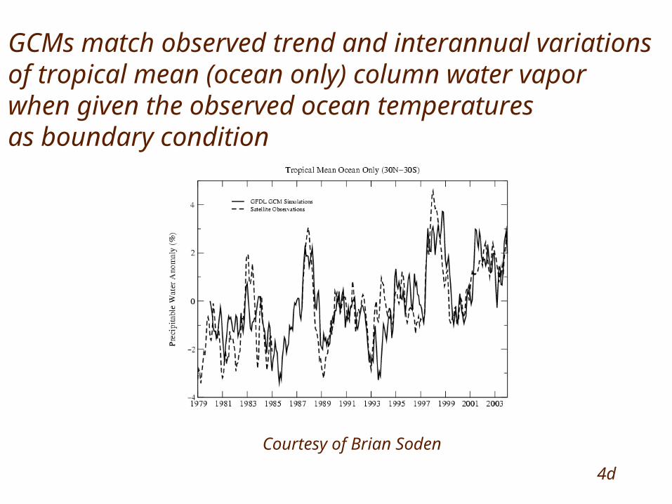
GCMs match observed trend and interannual variations of tropical mean (ocean only) column water vapor when given the observed ocean temperatures as boundary condition
Courtesy of Brian Soden
4d

Local vertically integrated atmospheric moisture budget:
precipitation
evaporation
vertically integrated moisture flux vapor mixing ratio
4e

PCMDI/CMIP3
But response of global mean temperature is correlated (across GCMs)with the response of the poleward moisture flux responsible for the pattern
of subtropical decrease and subpolar increase in precipitation
Global mean T
% increase inpolewardmoisture fluxIn midlatitudes
4f
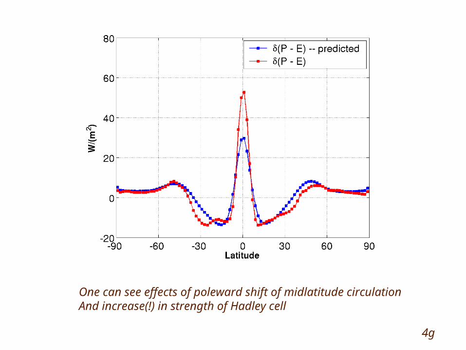
One can see effects of poleward shift of midlatitude circulationAnd increase(!) in strength of Hadley cell
4g

Temperature change
% P
reci
pita
tion
chan
ge
PCMDI -AR4 Archive
5
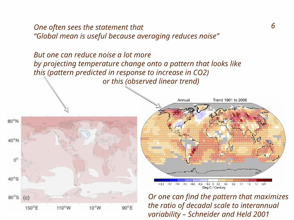
One often sees the statement that “Global mean is useful because averaging reduces noise”
But one can reduce noise a lot moreby projecting temperature change onto a pattern that looks like this (pattern predicted in response to increase in CO2) or this (observed linear trend)
Or one can find the pattern that maximizesthe ratio of decadal scale to interannualvariability – Schneider and Held 2001
6

“The global mean surface temperature has an especially simple relationship with the global mean TOA energy balance” ??
€
F(θ) = β (θ,ξ )δT∫ (ξ )dξ
< F >≡ F(θ)dθ = B(ξ )T(ξ )dξ∫∫ ; B(ξ ) = β (θ,ξ )dθ∫
if δT(θ) = f (θ) < T > then < F >= ˜ B < T >
˜ B ≡ B(ξ ) f (ξ )dξ∫
Seasonal OLR vs Surface Tat different latitudes
Seasonal OLR vs 500mb Tat different latitudes
Most general linear OLR-surfaceT relation
Relation between global means depends on spatial structure7
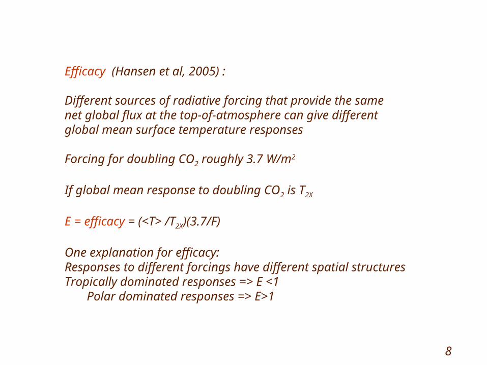
Efficacy (Hansen et al, 2005) :
Different sources of radiative forcing that provide the samenet global flux at the top-of-atmosphere can give differentglobal mean surface temperature responses
Forcing for doubling CO2 roughly 3.7 W/m2
If global mean response to doubling CO2 is T2X
E = efficacy = (<T> /T2X)(3.7/F)
One explanation for efficacy:Responses to different forcings have different spatial structuresTropically dominated responses => E <1 Polar dominated responses => E>1
8
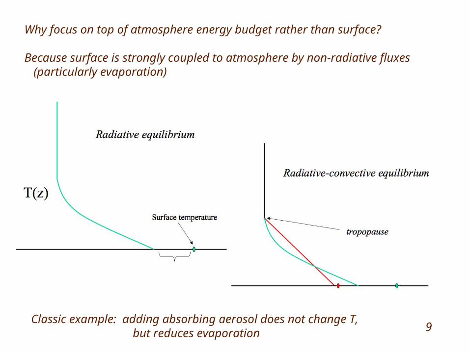
Why focus on top of atmosphere energy budget rather than surface?
Because surface is strongly coupled to atmosphere by non-radiative fluxes (particularly evaporation)
Classic example: adding absorbing aerosol does not change T, but reduces evaporation 9

If net solar flux does not change, outgoing IR does not change either (in equilibrium), -- with increased CO2, atmosphere is more opaque to infrared photons=> average level of emission to space moves upwards, maintaining same T=> warming of surface, given the lapse rate
Final response depends on how other absorbers/reflectors (esp. clouds, water vapor, surface snow and ice)
change in response to warming due to CO2, and on how the mean lapse rate changes 10

Equilibrium climate sensitivity:Double the CO2 and wait for the system to equilibrate
But what is the “system”? glaciers? “natural” vegetation? Why not specify emissions rather than concentrations?
Transient climate sensitivity:Increase CO2 1%/yr and examine climate at the time of doubling
t
CO2 forcing
Heat uptake by deep ocean
W/m2
~3.7
Typical setup – increase till doubling – then hold constant
After CO2 stabilized, warming of near surface can be thought of as due to reduction in heat uptake
T response
11

“Observational constraints” on climate sensitivity (equilibrium or transient)
Model (a,b,c,…)
Simulates some observed phenomenon: comparison with simulation constrains a,b,c …
predicts climate sensitivity;depends on a,b,c,…
Model can be GCM – in which case constraint can be rather indirect(constraining processes of special relevance to climate sensitivity)
Or it can be simple model in which climate sensitivity is determined by 1 or 2 parameters.
12
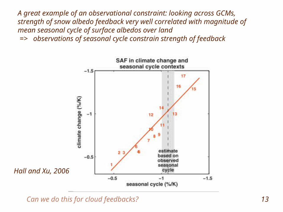
Hall and Xu, 2006
A great example of an observational constraint: looking across GCMs, strength of snow albedo feedback very well correlated with magnitude ofmean seasonal cycle of surface albedos over land => observations of seasonal cycle constrain strength of feedback
Can we do this for cloud feedbacks? 13

€
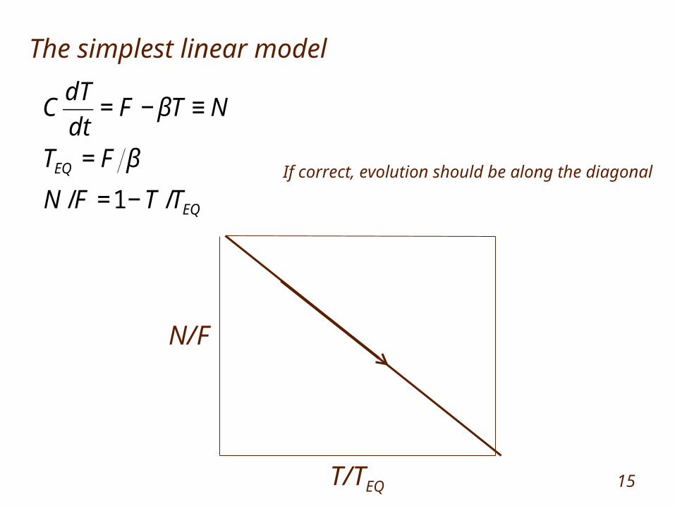
CdT
dt= F − βT ≡ N
TEQ = F β
The simplest linear model
The left-hand side of this equation (the ocean model) is easy to criticize, but what about the right hand side?
forcing
Heat uptake
14
€
CdT
dt= F − βT ≡ N
TEQ = F β
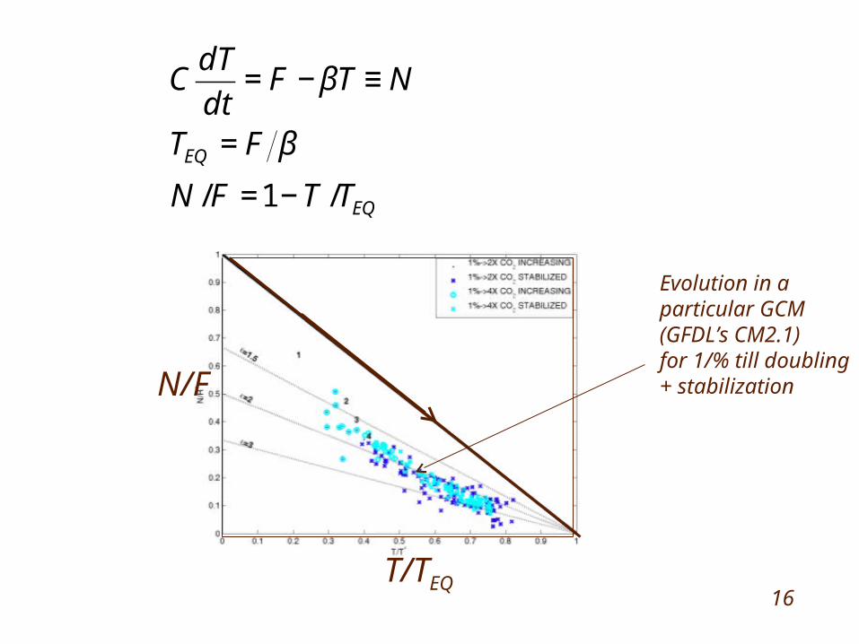
N /F =1− T /TEQ
N/F
T/TEQ
The simplest linear model
If correct, evolution should be along the diagonal
15
€
CdT
dt= F − βT ≡ N
TEQ = F β
N /F =1− T /TEQ
N/F
T/TEQ
Evolution in aparticular GCM(GFDL’s CM2.1)for 1/% till doubling+ stabilization
16

€
CdT
dt= F − βT ≡ N
TEQ = F β
N /F =1− T /TEQ
N/F
T/TEQ
€
βT = F − N
replaced by
βT = F − EN N
EN=2
The efficacy of heat uptake >1 since it primarily affects subpolarlatitudes
Transient sensitivity affectedby efficacy as well as magnitude of heat uptake
17
N/F
T/TEQ
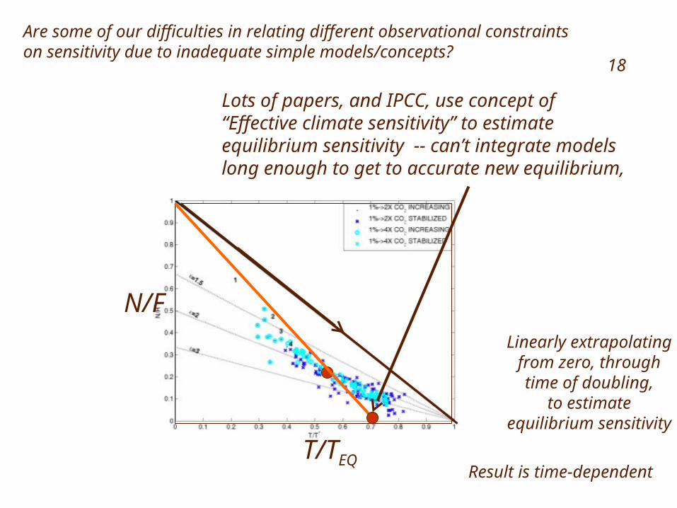
Lots of papers, and IPCC, use concept of “Effective climate sensitivity” to estimateequilibrium sensitivity -- can’t integrate modelslong enough to get to accurate new equilibrium,
Linearly extrapolatingfrom zero, throughtime of doubling,
to estimateequilibrium sensitivity
Result is time-dependent
Are some of our difficulties in relating different observational constraintson sensitivity due to inadequate simple models/concepts?
18
2 43 51
2
1.5
2.5
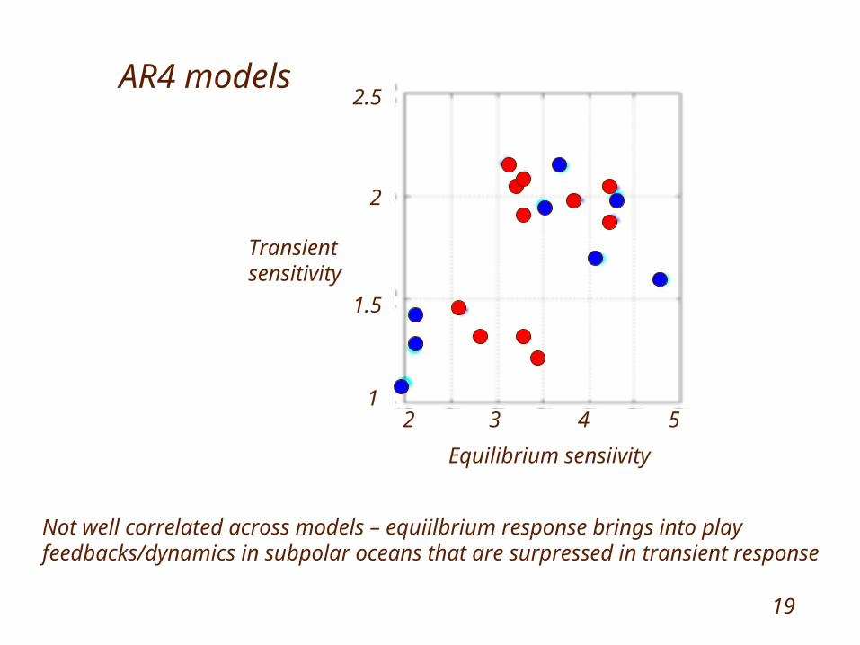
Equilibrium sensiivity
AR4 models
Transientsensitivity
Not well correlated across models – equiilbrium response brings into play feedbacks/dynamics in subpolar oceans that are surpressed in transient response
19
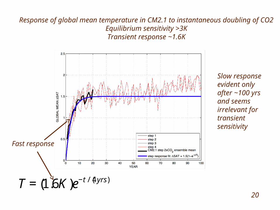
Response of global mean temperature in CM2.1 to instantaneous doubling of CO2Equilibrium sensitivity >3KTransient response ~1.6K
€
T = (1.6K)e−t /(4 yrs)
Fast response
Slow responseevident onlyafter ~100 yrsand seems irrelevant fortransient sensitivity
20
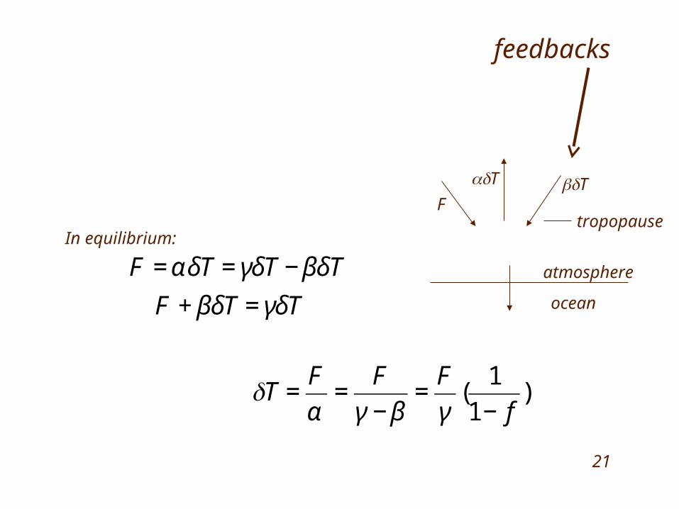
€
F = αδT = γδT − βδT
F + βδT = γδT
€
δT =F
α=
F
γ − β=
F
γ(
1
1− f)
tropopauseF
δT βδT
atmosphere
ocean
In equilibrium:
feedbacks
21

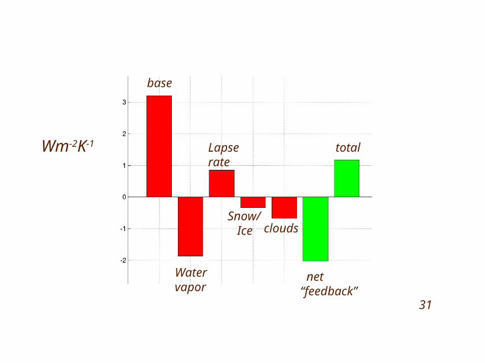
base
Lapserate
Snow/ Ice
Watervapor
clouds
net“feedback”
totalWm-2K-1
Positivefeedback
Global mean feedback analysis for CM2.1 (in A1B scenario over 21st century)
Base in isolation would give sensitivity of ~1.2KFeedbacks convert this to ~3K 22
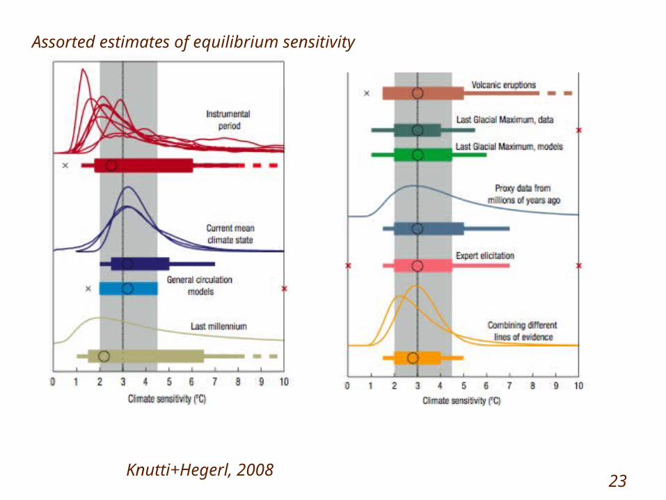
Knutti+Hegerl, 2008
Assorted estimates of equilibrium sensitivity
23

24

Roe-Baker
Gaussian distribution of f => skewed distribution of 1/(1-f)
25
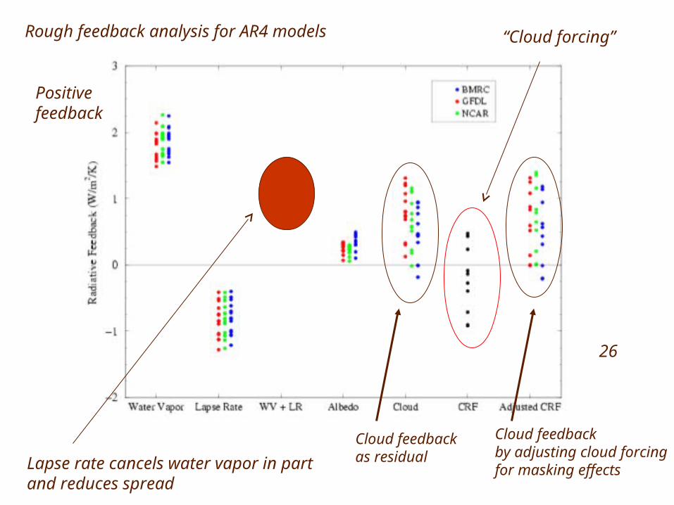
Cloud feedback as residual
Cloud feedback by adjusting cloud forcingfor masking effects
Positivefeedback
Rough feedback analysis for AR4 models “Cloud forcing”
Lapse rate cancels water vapor in partand reduces spread
26

€
R = (1− f )(α + βw1)
€
δR = δC R + δW R
δC R = −(α + βw1)δf
δW R = (1− f )βδw1
€
CRF = − f (α + βw2)
δCRF = −(α + βw2)δf − fβδw2
€
f
€
1− f
0
€
+βw1
€
w1
€
w2
Cloud forcing
Cloud feedback
Water vapor feedback
Cloud feedback is different from change in cloud forcing
27
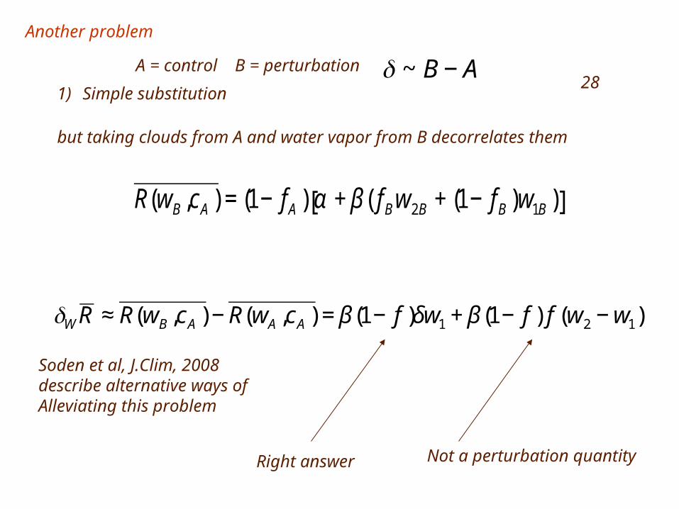
€
R(wB ,cA ) = (1− fA ) α + β ( fB w2B + (1− fB )w1B )[ ]
€
δW R ≈ R(wB ,cA ) − R(wA ,cA ) = β (1− f )δw1 + β (1− f ) f (w2 − w1)
1) Simple substitution
but taking clouds from A and water vapor from B decorrelates them
Not a perturbation quantity
€
δ ~ B − A
Right answer
A = control B = perturbation
Another problem
Soden et al, J.Clim, 2008describe alternative ways ofAlleviating this problem
28
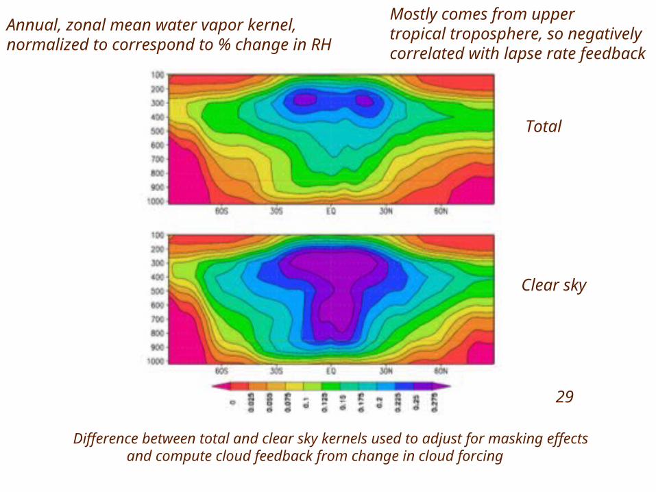
Annual, zonal mean water vapor kernel, normalized to correspond to % change in RH
Total
Clear sky
Difference between total and clear sky kernels used to adjust for masking effects and compute cloud feedback from change in cloud forcing
Mostly comes from uppertropical troposphere, so negativelycorrelated with lapse rate feedback
29

Courtesy of B. SodenNet cloud feedbackfrom 1%/ yr CMIP3/AR4simulations
SW
and
LW
clo
ud f
eedb
ack
LW feedbacks positive (FAT hypothesis? => Dennis’s lecture)SW feedbacks positive/negative, and correlated with total
30
base
Lapserate
Snow/ Ice
Watervapor
clouds
net“feedback”
totalWm-2K-1
31

alternative choices of starting point(not recommended)
€
a
1− f=
b
1− ′ f
b = aξ
′ f =1−ξ + ξf
Weak negative“lapse rate feedback”
Very strong negative“free tropospheric feedback”
Choice of “base” = “no feedback” is arbitrary!
32
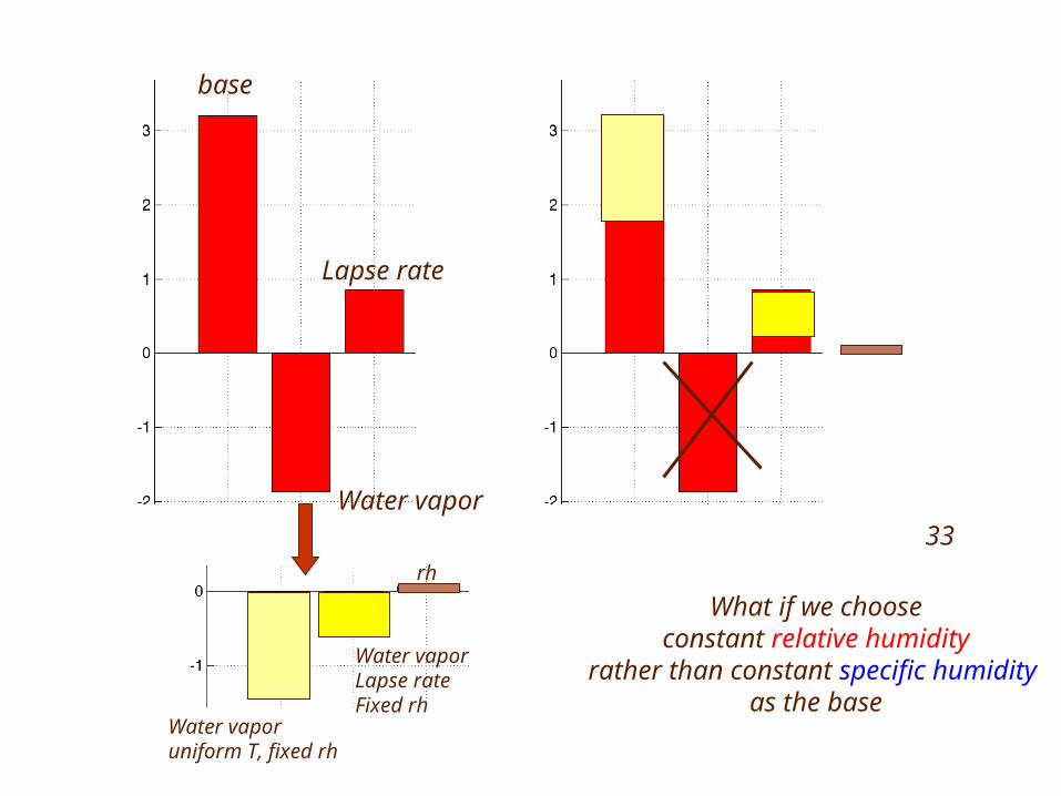
base
rh
Water vaporLapse rateFixed rh
Water vaporuniform T, fixed rh
Lapse rate
Water vapor
What if we chooseconstant relative humidity
rather than constant specific humidity as the base
33
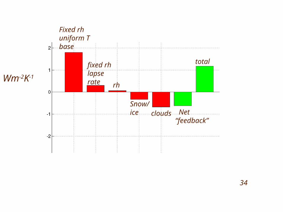
Fixed rhuniform Tbase
fixed rhlapserate rh
Snow/ice clouds Net
“feedback”
total
Wm-2K-1
34

3.3
1.85 clouds
Non-dimensional version
Clouds look like they have increased in importance (since water vapor change due to temperature changeresulting from cloud change is now charged to the “ cloud” account}
Net feedback
total
35
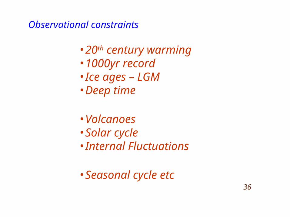
Observational constraints
•20th century warming•1000yr record •Ice ages – LGM•Deep time
•Volcanoes•Solar cycle•Internal Fluctuations
•Seasonal cycle etc36
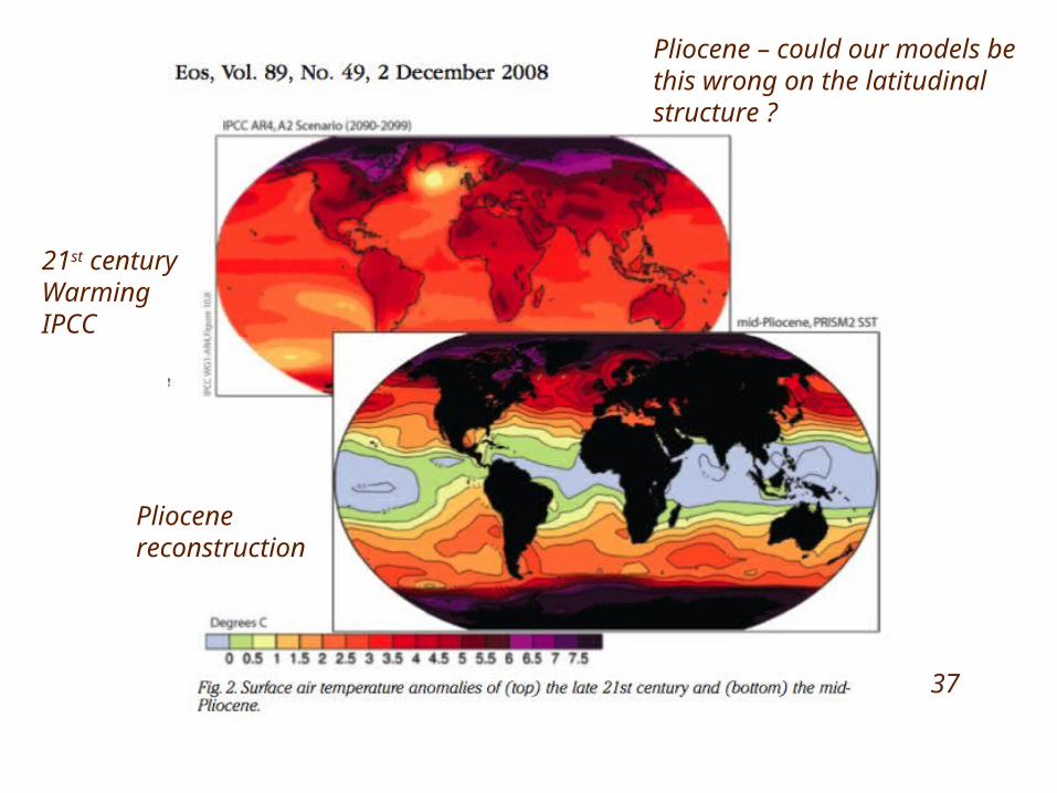
Pliocene – could our models bethis wrong on the latitudinalstructure ?
21st centuryWarmingIPCC
Pliocenereconstruction
37
38www.globalwarmingart.com
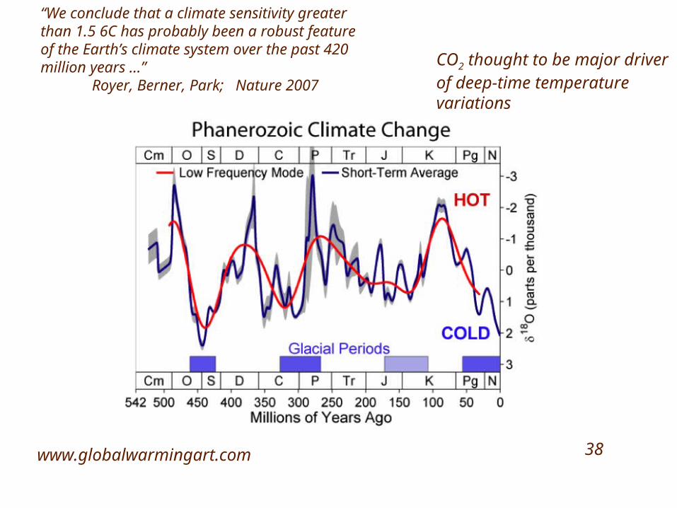
“We conclude that a climate sensitivity greater than 1.5 6C has probably been a robust feature of the Earth’s climate system over the past 420 million years …” Royer, Berner, Park; Nature 2007
CO2 thought to be major driverof deep-time temperaturevariations

39
www.globalwarmingart.com

Global mean cooling due to Pinatubo volcanic eruption
Range of ~10 ModelSimulationsGFDL CM2.1
Courtesy of G Stenchikov
Observationswith El Ninoremoved
Relaxation time after abrupt cooling contains information on climate sensitivity
40

Yokohata, et al, 2005
Low sensitivity model
High sensitivity model
Pinatubo simulation
41

Observed total solar irradiance variations in 11yr solar cycle (~ 0.2% peak-to-peak)
42

Tung et al => 0.2K peak to peak(other studies yield only 0.1K)
Seems to imply large transient sensitivity
4 yr damping time
1.8K (transient) sensitivity
Only gives 0.05 peak to peak
43
www.globalwarmingart.com
44
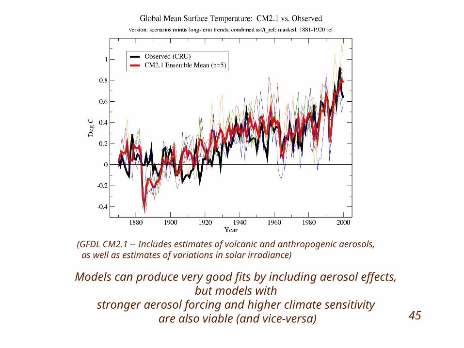
(GFDL CM2.1 -- Includes estimates of volcanic and anthropogenic aerosols, as well as estimates of variations in solar irradiance)
Models can produce very good fits by including aerosol effects, but models with
stronger aerosol forcing and higher climate sensitivity are also viable (and vice-versa) 45
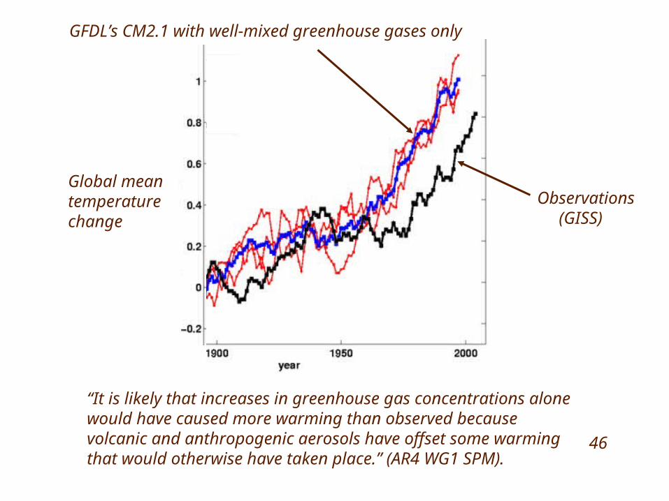
“It is likely that increases in greenhouse gas concentrations alone would have caused more warming than observed because volcanic and anthropogenic aerosols have offset some warming that would otherwise have taken place.” (AR4 WG1 SPM).
Observations (GISS)
GFDL’s CM2.1 with well-mixed greenhouse gases only
Global mean temperature change
46
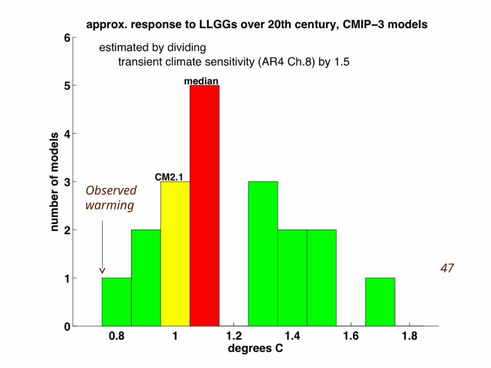
Observedwarming
47

Kiehl, 2008: In AR4, forcing over 20th century and equilibrium climate sensitivity negatively correlated
How would this look for transient climate sensitivity?
48

http://data.giss.nasa.gov/gistemp/
Do interhemispheric differences in warming provide a simple testof aerosol forcing changes over time?
49
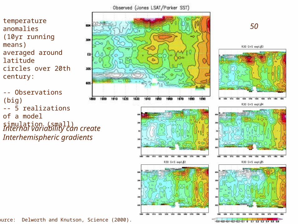
temperature anomalies (10yr running means)averaged around latitude circles over 20th century: -- Observations (big)-- 5 realizations of a model simulation (small)
Source: Delworth and Knutson, Science (2000).
Internal variability can createInterhemispheric gradients
50

OLR
SW down
SW up
total
Forcing computed from differencing TOA fluxes in two runs of a model (B-A)B = fixed SSTs with varying forcing agents; A fixed SSTs and fixed forcing agents
51
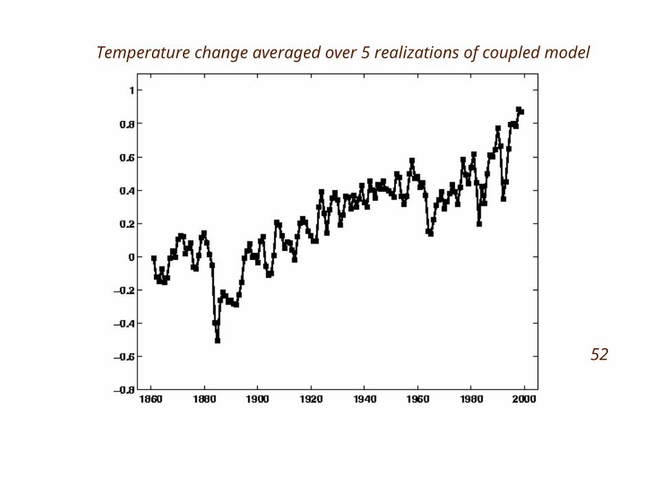
Temperature change averaged over 5 realizations of coupled model
52
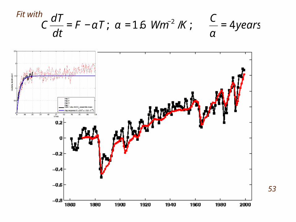
€
CdT
dt= F −αT; α =1.6 Wm−2 /K;
C
α= 4years
Fit with
53

Forcing with no damping
Forcing (with no damping) fits the trend well, if you use transient climate sensitivity, which takes into account magnitude/efficacy of heat uptake
54

€
c∂T
∂t= S + N −αT
S
TN
c
Spenser-Braswell, 2008
Suppose N isTOA noise, but correlated with T because it forces T
Regressing flux with T
€
−(N −αT)T
T 2= ′ α
′ α = αS2
N 2 + S2< α
Why can’t we just look at the TOA fluxes and surface temperatures?TOA record is short,But there are other issues
If S and N are uncorrelatedand have the same spectrumone can show that
(Assuming no forcing)
55

Shortwave regression across ensemble, following K. Swanson 2008
Wm-2K-1
All-forcing20th century
Following an idea of K. Swanson, take a set of realizations of the 20th century from one model, and correlate global mean TOA with surface temperature across the ensemble
56

Shortwave regression across ensemble, following K. Swanson 2008
All-forcing20th century
A1B scenario
Wm-2K-1
Is this a sign of non-linearity? What is this?
57

Shortwave regression across ensemble, following K. Swanson 2008
All-forcing20th centuryWm-2K-1
A1B scenario
90%
Estimate of noise in this statistic from 2000yr control run58
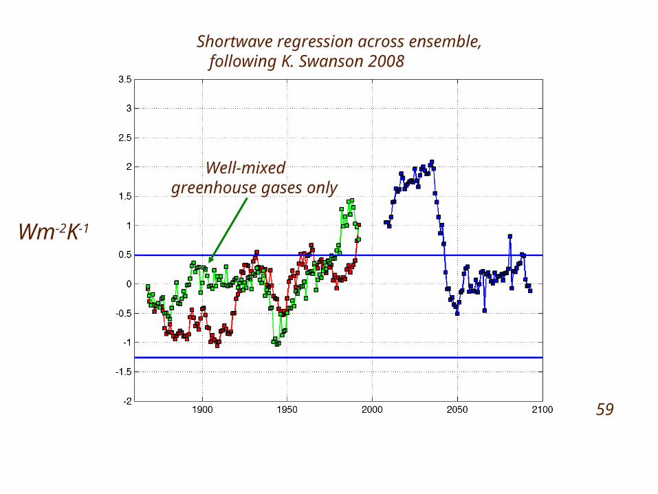
Shortwave regression across ensemble, following K. Swanson 2008
Wm-2K-1
Well-mixedgreenhouse gases only
59
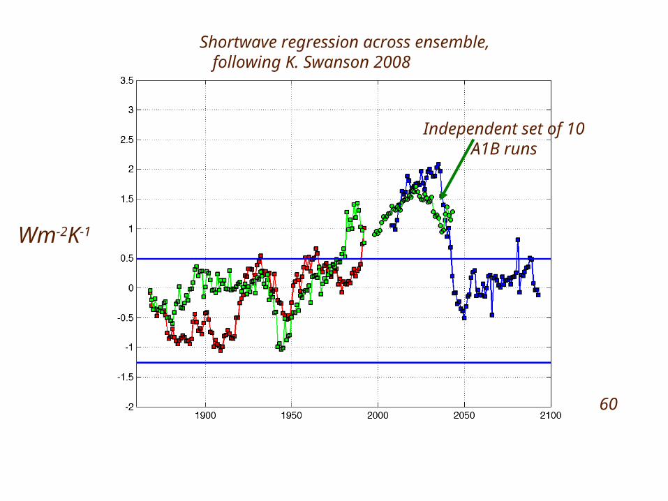
Shortwave regression across ensemble, following K. Swanson 2008
Wm-2K-1
Independent set of 10 A1B runs
60
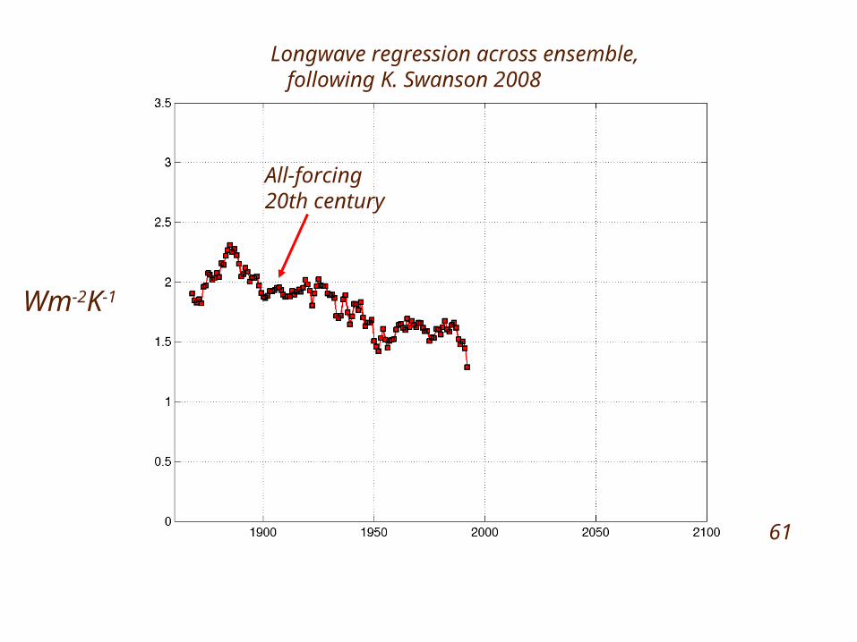
Longwave regression across ensemble, following K. Swanson 2008
Wm-2K-1
All-forcing20th century
61
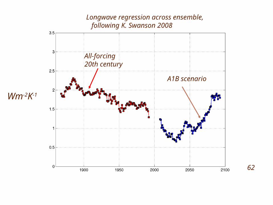
Longwave regression across ensemble, following K. Swanson 2008
Wm-2K-1
All-forcing20th century
A1B scenario
62

Longwave regression across ensemble, following K. Swanson 2008
Wm-2K-1
63
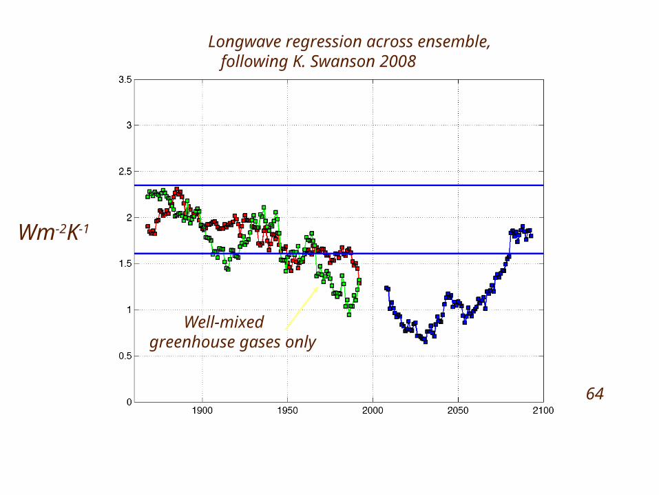
Longwave regression across ensemble, following K. Swanson 2008
Wm-2K-1
Well-mixedgreenhouse gases only
64
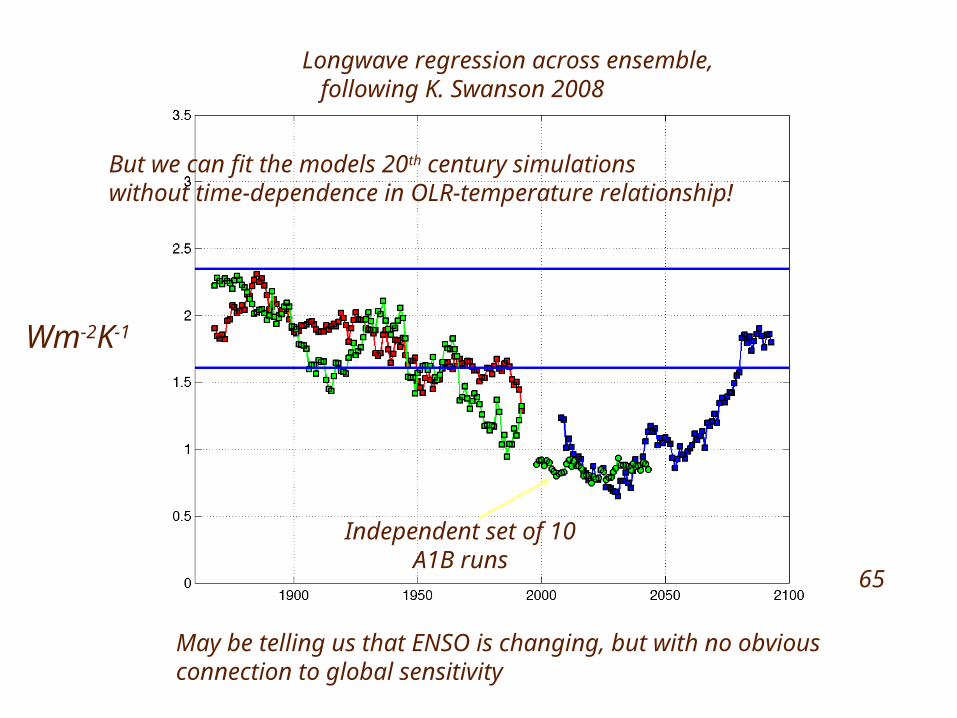
Longwave regression across ensemble, following K. Swanson 2008
Wm-2K-1
Independent set of 10 A1B runs
But we can fit the models 20th century simulations without time-dependence in OLR-temperature relationship!
May be telling us that ENSO is changing, but with no obviousconnection to global sensitivity
65
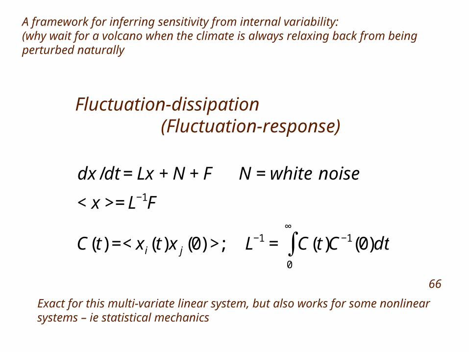
Fluctuation-dissipation (Fluctuation-response)
€
dx /dt = Lx + N + F N = white noise
< x >= L−1F
C(t) =< x i(t)x j (0) >; L−1 = C(t)C−1(0)dt0
∞
∫
A framework for inferring sensitivity from internal variability:(why wait for a volcano when the climate is always relaxing back from beingperturbed naturally
Exact for this multi-variate linear system, but also works for some nonlinearsystems – ie statistical mechanics
66
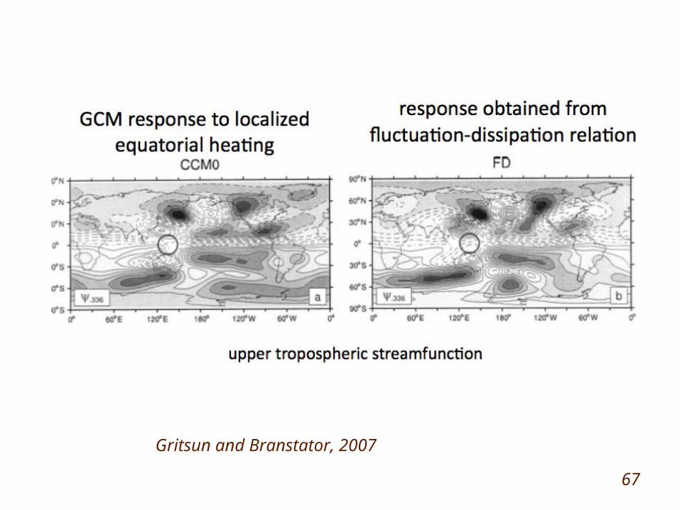
Gritsun and Branstator, 2007
67
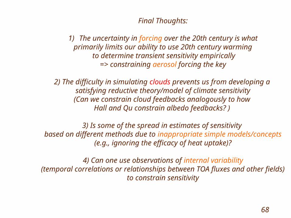
Final Thoughts:
1) The uncertainty in forcing over the 20th century is whatprimarily limits our ability to use 20th century warming
to determine transient sensitivity empirically=> constraining aerosol forcing the key
2) The difficulty in simulating clouds prevents us from developing a satisfying reductive theory/model of climate sensitivity
(Can we constrain cloud feedbacks analogously to how Hall and Qu constrain albedo feedbacks? )
3) Is some of the spread in estimates of sensitivity based on different methods due to inappropriate simple models/concepts
(e.g., ignoring the efficacy of heat uptake)?
4) Can one use observations of internal variability(temporal correlations or relationships between TOA fluxes and other fields)
to constrain sensitivity
68

Supplementary figures

(C. Keeling)
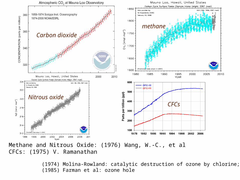
Methane and Nitrous Oxide: (1976) Wang, W.-C., et alCFCs: (1975) V. Ramanathan (1974) Molina-Rowland: catalytic destruction of ozone by chlorine; (1985) Farman et al: ozone hole
Carbon dioxide
methane
Nitrous oxideCFCs
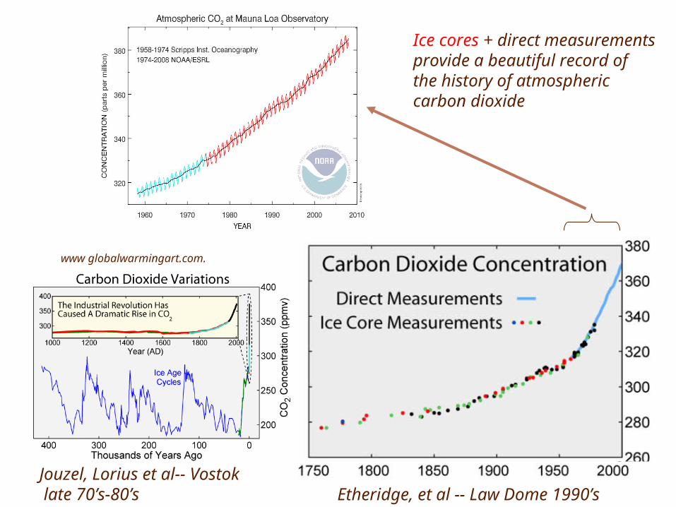
Jouzel, Lorius et al-- Vostok late 70’s-80’s Etheridge, et al -- Law Dome 1990’s
Ice cores + direct measurementsprovide a beautiful record of the history of atmosphericcarbon dioxide
www globalwarmingart.com.

Carbon dioxide
methane
Nitrous oxide
CFCsother
http://www.esrl.noaa.gov/gmd/aggi/

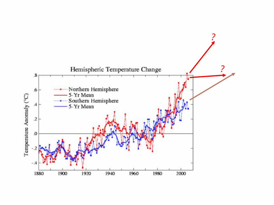
Was the 20th century warming
1) primarily forced by increasing greenhouse gases?
or,
2) primarily forced by something else?
or,
3) primarily an internal fluctuation of the climate?
Claim: Our climate theories STRONGLY support 1)
A central problem for the IPCC has been to evaluate this claimand communicate our level of confidence appropriately

Global ocean heat content
1955 20051980
Energy is going into ocean=>More energy is entering the atmosphere from space than isgoing out
Almost all parts of the Earth’ssurface have warmed over the past 100 years
IPCC 4th Assessment Report.
www.globalwarmingart.com

IPCC AR4 WG1 Summary for Policymakers
?
?
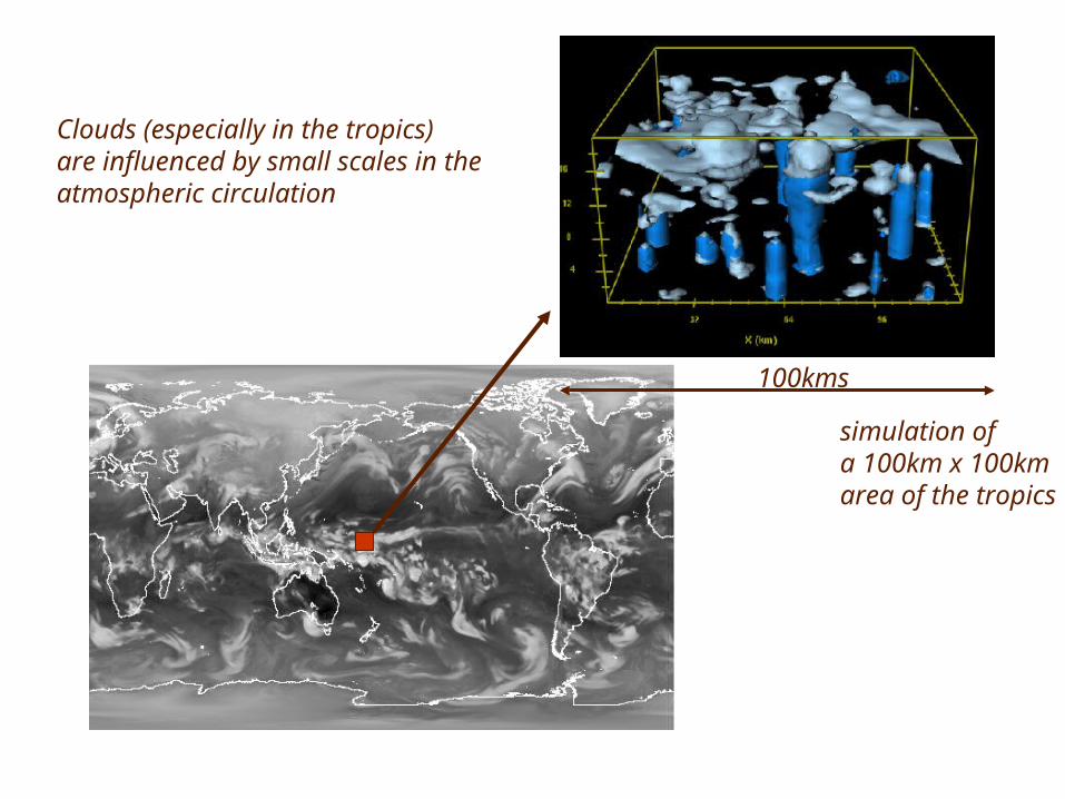
100kms
Clouds (especially in the tropics)are influenced by small scales in the atmospheric circulation
simulation of a 100km x 100kmarea of the tropics
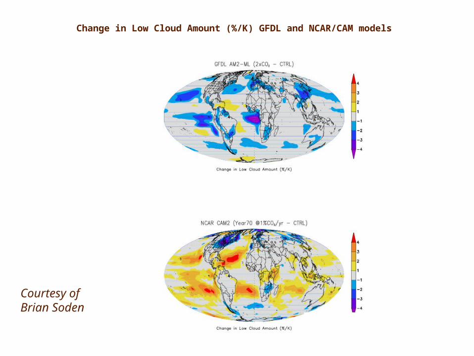
Change in Low Cloud Amount (%/K) GFDL and NCAR/CAM models
Courtesy of Brian Soden

Total Column Water Vapor Anomalies (1987-2004)
Held and Soden J.Clim. 2006
We have high confidence in the model projections of increased water vapor.