Climatic radiowave propagation models for the design ofsatellite communication systemsvan de Kamp, M.M.J.L.

DOI:10.6100/IR527715

Published: 01/01/1999

Document VersionPublisher’s PDF, also known as Version of Record (includes final page, issue and volume numbers)

Please check the document version of this publication:

• A submitted manuscript is the author's version of the article upon submission and before peer-review. There can be important differencesbetween the submitted version and the official published version of record. People interested in the research are advised to contact theauthor for the final version of the publication, or visit the DOI to the publisher's website.• The final author version and the galley proof are versions of the publication after peer review.• The final published version features the final layout of the paper including the volume, issue and page numbers.

Link to publication

General rightsCopyright and moral rights for the publications made accessible in the public portal are retained by the authors and/or other copyright ownersand it is a condition of accessing publications that users recognise and abide by the legal requirements associated with these rights.

• Users may download and print one copy of any publication from the public portal for the purpose of private study or research. • You may not further distribute the material or use it for any profit-making activity or commercial gain • You may freely distribute the URL identifying the publication in the public portal ?

Take down policyIf you believe that this document breaches copyright please contact us providing details, and we will remove access to the work immediatelyand investigate your claim.

Download date: 26. Aug. 2018

Climatic Radiowave Propagation Modelsfor the design of

Satellite Communication Systems

PROEFSCHRIFT

ter verkrijging van de graad van doctoraan de Technische Universiteit Eindhoven,

op gezag van de Rector Magnificus, prof. dr. M. Rem,voor een commissie aangewezen door het College voor Promoties

in het openbaar te verdedigenop woensdag 24 november 1999 om 16:00 uur

door

Maximilianus Maria Josephus Leonardus van de Kamp

geboren te Driebergen

Dit proefschrift is goedgekeurd door de promotoren:

prof.dr.ir. G. Brussaardenprof.dr. E.T. Salonen

Copromotor:dr.ir. M.H.A.J. Herben

CIP-DATA LIBRARY TECHNISCHE UNIVERSITEIT EINDHOVEN

Kamp, Maximilanus M.J.L. van de

Climatic radiowave propagation models for the design of satellite communication systems /by Maximilianus M.J.L. van de Kamp. - Eindhoven : Technische Universiteit Eindhoven,1999.Proefschrift. - ISBN 90-386-1700-3NUGI 832Trefw.: radiogolfvoortplanting / elektromagnetische golven ; depolarisatie /radiogolven ; troposfeer / satellietcommunicatie / microgolfvoortplanting ; atmosfeer.Subject headings: radiowave propagation / tropospheric electromagnetic wave propagation /rain / electromagnetic wave absorption / satellite communication.

Cover illustration painted by Marie-Thérèse van de Kamp

© 1999 by M.M.J.L. van de Kamp, Eindhoven

All rights reserved. No part of this publication may be reproduced or transmitted in any formor by any means, electronic, mechanical, including photocopy, recording, or any informationstorage and retrieval system, without the prior written permission of the copyright owner.

Rows and flows of angel hair,and ice-cream castles in the air,and feather canyons everywhere:I’ve looked at clouds that way.

But now they only block the sun,they rain and snow on everyone.So many things I would have done,but clouds got in my way.

I’ve looked at clouds from both sides now:from up and down, and still somehow,it’s cloud illusions I recall;I really don’t know clouds at all.

Joni Mitchell

AbstractThe quality of satellite communication systems can be seriously affected by variable climaticphenomena such as rain and turbulence. For the design of communication systems with arequired availability, statistical knowledge of climatic propagation effects is essential.

In this thesis three climatic propagation effects are studied:• the fade slope (rate of change) of attenuation due to rain;• scintillation due to tropospheric turbulence;• depolarisation due to rain and ice crystals.

For the study, experimental satellite signal measurements are analysed, received from thesatellite Olympus at Eindhoven University of Technology and Helsinki University ofTechnology. The statistical behaviour of the propagation effects is studied in relation with thetheoretical background. The results obtained are compared with results from many othermeasurement sites. This way, relations with link parameters (among which the frequency) andwith meteorological parameters are studied. New prediction models for the propagationeffects are developed, as well as improvements to existing models. The main conclusionsobtained are the following:

The rain fade slope is found to have, conditional for a rain attenuation level, a symmetricaldistribution. The standard deviation of this distribution is proportional with attenuation,independent of frequency, and dependent on filter bandwidth. It is likely to depend onelevation angle and on the relative contribution of different rain types.

The signal level due to tropospheric scintillation is found to have an asymmetricaldistribution; the asymmetry increases with scintillation intensity. The frequency dependenceof scintillation shows strong variability between different measurement sites; several possibleexplanations for this observation are given. For global long-term prediction of scintillation,current models use only the wet term of refractivity as a meteorological input, however it isfound that the water content of heavy clouds is necessary as an additional meteorologicalinput parameter. An improved prediction model of tropospheric scintillation is presented,based on the conclusions found.

The relation between depolarisation and attenuation due to rain is studied using measurementsfrom many different sites; the different dependencies of this relation on link parameters areempirically quantified and the model for this relation is updated. For the case of depolarisationcaused by simultaneous rain and ice, a calculation method is developed to separate thecontributions of both partial media.

The conclusions obtained and the new prediction models developed in this thesis can improvethe prediction of propagation effects, which is essential for satellite communication systemdesign in general and for adaptive link control systems in particular.

5

ContentsList of symbols 9Subscripts 11Abbreviations and acronyms 11

1. Introduction 131.1. Communication in the Ka- and V-bands 131.2. Propagation effects 13

1.2.1. Rain attenuation 131.2.2. Scintillation 141.2.3. Depolarisation 15

1.3. Brief survey of this thesis 16

2. Adaptive Link Control 172.1. Introduction 172.2. Adaptive Power Control 17

2.2.1. Introduction 172.2.2. Up-Link Power Control 182.2.3. Down-Link Power Control 202.2.4. Up/Down-Link Power Control 212.2.5. Summary 23

2.3. Adaptive Depolarisation Cancellation 242.3.1. Introduction 242.3.2. Dynamic cancellation 242.3.3. Forward cancellation 262.3.4. Static cancellation 272.3.5. Compensation at baseband 27

2.4. Required propagation information 282.4.1. Required information for Adaptive Power Control 282.4.2. Required information for Adaptive Depolarisation Cancellation 292.4.3. Dependence on fade margin 30

3. The Olympus Propagation Experiment 313.1. The Olympus satellite 313.2. The measurement site in Kirkkonummi 32

3.2.1. Measurement set-up 323.2.2. Data sets 33

3.3. The measurement site in Eindhoven 343.3.1. Measurement set-up 343.3.2. Data set 35

4. Fade slope 374.1. Introduction 374.2. Measurement analysis 38

4.2.1. Measurement results 384.2.2. Time symmetry 394.2.3. Attenuation dependent distribution model 424.2.4. Dependence on rain type 45

6

4.2.5. Dependence on filter bandwidth 464.3. Comparison with other sites 494.4. Conclusions 55

5. Scintillation 575.1. Introduction 575.2. Theory of tropospheric scintillation 58

5.2.1. Wave propagation in the turbulent atmosphere 585.2.2. Short-term signal fluctuations 595.2.3. Distribution of standard deviation 625.2.4. Prediction models 64

5.2.4.1. Models for long-term standard deviation 645.2.4.2. Models for signal level distribution 66

5.3. Statistical measurement results from Kirkkonummi 705.3.1. Distribution of variance 705.3.2. Distribution of signal level 73

5.3.2.1. Comparison with current distribution models 735.3.2.2. Improved model 75

5.4. Dependence on link parameters 835.4.1. Frequency dependence 83

5.4.1.1. Numerical result from the measurements 835.4.1.2. Numerical results from measurements in Spino d'Adda 865.4.1.2. Comparison with other sites 885.4.1.4. Discussion 91

5.4.2. Polarisation angle dependence 965.5. Relation with meteorological parameters 97

5.5.1. Long-term correlation with the wet term of refractivity 975.5.2. Diurnal correlation with cloud information 1005.5.3. Improved long-term prediction models 104

5.6. Relation with rain attenuation and total fade 1175.6.1. Relation with attenuation 1175.6.2. Combining scintillation and attenuation 121

5.7. Conclusions 125

6. Depolarisation 1276.1. Introduction 1276.2. Modelling theory of rain depolarisation 1296.3. Relation between XPD and CPA due to rain 132

6.3.1. A model 1326.3.2. Measurement results from Eindhoven 1346.3.3. Measurement results from other sites 1386.3.4. Experimental verification of the model 140

6.3.4.1. Elevation angle dependence 1406.3.4.2. Polarisation orientation dependence 1426.3.4.3. Frequency dependence 1436.3.4.4. Polarisation angle dependence 1466.3.4.5. Frequency dependence at higher frequencies 1496.3.4.6. General update of the model 151

6.4. Anisotropy and canting angle of rain 1536.4.1. Introduction 153

7

6.4.2. Practical formulae 1536.4.3. Theoretical relations of anisotropy 1546.4.4. Selection of pure rain events 1566.4.5. Experimental results 157

6.5. Depolarisation due to ice crystals 1626.5.1. Introduction and theory 1626.5.2. Calculation method of anisotropy and canting angle 1636.5.3. Selection of pure ice events 1636.5.4. Experimental results 163

6.6. Depolarisation due to a combination of rain and ice 1666.6.1. Introduction 1666.6.2. Model as a cascade of two media 1666.6.3. Separation method 1686.6.4. Experimental test of separation method 175

6.7. Statistics of depolarisation 1816.7.1. Statistics of XPD and CPA 1816.7.2. Relative occurrences of rain, ice and combination 184

6.8. Conclusions 187

7. Conclusions 189

8. References 193

Appendix A. Measurement procedures at other sites 207A.1. Measurements used in Chapter 4 (fade slope) 207A.2. Measurements used in Chapter 5 (scintillation) 208A.3. Measurements used in Chapter 6 (depolarisation) 213

Appendix B. Sensitivity evaluation of scintillation 217

Samenvatting (Nederlands) 221

Acknowledgment 223

Curriculum Vitae 225

8

9

List of Symbolsa ( ) parameterae (m) effective radius of the earth = 8.5×106m at sea levelA (dB) attenuationAr (dB) characteristic parameter of rain depolarisationb ( ) parameterBi (º) characteristic parameter of ice depolarisationc (m s-1) velocity of light = 299 792 458 m s-1 in vacuumC (dB) parameter of XPD - CPA modelCb (%) Cumulonimbus cloud amountCn

2 ( ) structure constant of refractive index fluctuationsC/N (dB) carrier-to-noise ratioCPA (dB) CoPolar AttenuationCPL (dB) CoPolar LevelCu (%) Cumulus cloud amountD (m) antenna diameterDe (m) effective antenna diametere ( ) 2.71828182845904...E (V/m) electric field strengthE0 (V/m) electric field strength amplitudeEr (%) errorf (GHz) (Hz)frequencyfB (Hz) filter bandwidthfs (Hz) sample frequencyF0 ( ) fraction of non-spherical raindropsg(De) ( ) aperture averaging function of scintillationG (dB) parameter of XPD - CPA modelh (m) height of the turbulent layerhw (m) height of water vapouri ( ) indexI0( ) ( ) modified Bessel function of 0th orderI (δ, σφ) (dB) parameter of XPD - CPA modelj ( ) imaginary unit ( −1 )k (m-1) wave numberl1,2,t (m) inner, outer and integral scale of turbulencelog 10-based logarithmln e-based logarithmL (m) (km) path length through turbulence or rainm meanM ( ) number of samplesN ( ) normalisation factorNwet (ppm) wet term of ground refractivityp( ) probability densityP ( ) (%) probabilityPhc (%) probability of heavy cloudsq ( ) parameterQ ( ) parameter for the long term scintillation standard deviation modelr parameter

10

R ( ) copolar ratioRr (mm/hr) rain intensityRH (%) relative humidityRCPL (dB) relative copolar signal level between polarisationss ( ) parameter of fade slope modelS (dB) parameter of XPD - CPA modelt (s) timeT (°C) temperature7 ( ) transmission matrixV (dB) parameter of XPD - CPA modelWhc (kg/m2) average water content of heavy cloudsx parameter

( )~x t random signalX ( ) polarisation ratioXPD (dB) Cross-Polarisation Discriminationy (dB) signal level deviation from the mean, due to scintillationye (dB) signal enhancement due to scintillationyf (dB) signal fade due to scintillationY ( ) polarisation ratioz (m) distanceα (dB) differential attenuationβ (º) differential phase shiftγ(P) (dB) partial signal level distributionΓ ( ) transmission coefficient ratioΓ( ) ( ) Gamma functionδ (º) polarisation angleδ(P) (dB) partial signal level distribution∆... step size of a parameterε (°) elevation angleζ (dB/s) fade slopeη ( ) antenna aperture efficiencyθ (º) angle from antenna axisλ (m) wavelengthξ ( ) parameter of short-term signal level distributionΞ ( ) parameter of double depolarising mediumπ ( ) 3.14159265358979323846264338327950288419716939937510582...σ standard deviationσ2 varianceσy

2 (dB2) variance of signal levelσs (º) spatial standard deviation of raindrop canting anglesσ2

tn (dB2) signal variance due to thermal noiseτ ( ) transmission coefficientφ (º) canting angleΦ (dB) antenna gainψ (º) relative phase between co- and crosspolar components of a signalψr (º) relative phase between copolar signalsΨ ( ) error coefficient

11

Subscripts

a attenuation / attenuatedi icelt long termn normalisedr rains scintillationt totalx quasi-horizontal polarisationy quasi-vertical polarisation

Abbreviations and acronyms

ACTS Advanced Communications Technology SatelliteADC Adaptive Depolarisation CancellationALC Adaptive Link ControlAPC Adaptive Power ControlBSE (Japanese Medium-Scale) Broadcasting Satellite for Experimental PurposesCOST COperation européenne dans le domaine de la recherche Scientifique et TechniqueCDIAC Carbon Dioxide Information Analysis CenterCDMA Code Division Multiple AccessDBOPEX Data Base of Olympus Propagation ExperimentersDBSG5 Data Base of Study Group 5 of ITU-RDLPC Down-Link Power ControlDSD Drop Size DistributionDSSS Direct-Sequence Spread SpectrumEIRP Effective Isotropically Radiated PowerESA European Space AgencyEUT Eindhoven University of TechnologyFDMA Frequency Division Multiple AccessHUT Helsinki University of TechnologyITU-R International Telecommunication Union - Radiocommunication SectorLEOS Low Earth Orbit SatelliteLHCP Left Hand Circularly PolarisedLPF Low-Pass FilterNASA National Aeronautics and Space AdministrationNCAR National Center for Atmospheric ResearchOPEX Olympus Propagation ExperimentOTS Orbital Test SatelliteQAM Quadrature Amplitude ModulationRHCP Right Hand Circularly PolarisedSCPC Single Channel Per CarrierTDMA Time Division Multiple AccessUDLPC Up- and Down-Link Power ControlULPC Up-Link Power ControlUTC Coordinated Universal TimeVSAT Very Small Aperture Terminal

12

13

1. Introduction

1.1. Communication in the Ka- and V-bands

The exploitation of satellit es for communication purposes has increased considerably duringthe last decades, in order to satisfy the growing demand for long-distance communications. Asthe C-band (4/6 GHz) is already congested, and the Ku-band (12/14 GHz) is filli ng up rapidly,recently interest focused on the utili sation of higher bands. Some systems are already designedto operate in the Ka-band (20/30 GHz), and it is probable that serious consideration will begiven soon to utilising the V-band (40/50 GHz).

The adoption of the Ka- and V-bands for satellit e links has many advantages. The bandsprovide plenty of bandwidth, which facilit ates the coordination of satellit e services and theintroduction of new communication services. Furthermore, antennas operating in these bandshave a higher directivity than antennas of equal size operating in lower frequency bands,which enables satellit es to be positioned closer together, since interference between adjacentsatellit es is reduced. In addition, the higher directivity facilit ates the use of high-gain spot-beam satellite antennas, thereby increasing down-link flux density and saving satellite power.

The performance of satellit e systems operating in the Ka- and V-bands essentially depends onthe propagation characteristics of the transmission medium. Effects due to the ionosphere canbe neglected at frequencies above 10 GHz. Tropospheric effects however, can cause signaldegradation on earth-space paths for substantial percentages of time, which leads to reductionin the quality and availabilit y of communication services. Some of the most importanttropospheric propagation effects are attenuation, depolarisation and scintill ation, which aredescribed in the next subsections. Some techniques have been developed to adaptivelycompensate these propagation impairments. These techniques are in this thesis generallyindicated as Adaptive Link Control (‘ALC’), and are described in Chapter 2.

1.2. Propagation effects

1.2.1. Rain attenuation

Attenuation on radio propagation paths is generally caused by various atmosphericcomponents: gases, water vapour, clouds, and rain. Rain attenuation, caused by scattering andabsorption by the water droplets, is one of the most fundamental limit ations to theperformance of satellit e communication links in the Ka-band, causing large variations in thereceived signal power, with littl e predictabilit y and many sudden changes. This kind of signalfading is also prevalent on earth-space links in the C- and Ku-bands, however, the depth offades in those frequency bands is small enough to be compensated for by including a smallfixed fade margin in the link budget in order to maintain the desired performance.

In the Ka- and V-bands, the attenuation caused by rain is too severe to be accounted for by afixed margin in the link budget. In order to provide the same performance as in the lowerfrequency bands, an excessively large margin would be required. Considering that this powermargin is needed only occasionally, this is clearly uneconomical. In addition, the powermargin needed would result in prohibitive requirements for satellit e power, and interference to

14

other communication systems operating at the same frequency band during clear-skyconditions.

To avoid these problems, alternative methods to reduce communication outage due to rainfading have been developed. These ‘f ade countermeasures’ compensate for rain attenuationadaptively, i.e. the quality of the link is improved when the signals are degraded. One of thesecountermeasures is Adaptive Power Control (‘APC’) , in which the transmitted power isincreased to compensate for fading due to rain on the propagation path. The techniques forthis are described further in Section 2.2.

Rain attenuation is, although an important signal impairment in the Ka- and V-bands, notdirectly studied in this thesis. This is because this phenomenon is already widely beingconsidered in many other studies and measurement campaigns, and the theoretical backgroundof rain attenuation is already relatively well understood. Alternatively, in this thesis oneparticular dynamic aspect of attenuation due to rain is studied: the fade slope, or the rate ofchange of attenuation due to rain. This is important for APC systems, to assess a requiredspeed with which the system can track attenuation changes.

1.2.2. Scintillation

The term “scintill ation” means fast fluctuations of signal amplitude and phase, caused byatmospheric turbulence. This effect is due to turbulent irregularities in temperature, humidityand pressure, which translate into small -scale variations in refractive index. Anelectromagnetic wave passing through this medium will t hen encounter various refraction andscattering effects, which will result in a multipath effect.

In the optical range, the influence of the temperature is dominant, resulting in, for instance,the twinkling of a star. In the microwave region, where the humidity fluctuations are moreimportant, the result is random degradation and enhancement in signal amplitude and phasereceived on a satellit e-earth link, as well as degradation in performance of large antennas,which can be noticed in particular in synthetic-aperture radars.

In general, the impact of rain attenuation on communication signals is predominant.Scintill ation, however, becomes important for low fade margin systems operating at highfrequencies and low elevation angles. In the Ka-band and above, and low elevation angles(≤≈ 15°), scintill ation may contribute as much as rain, or even more, to the total fademeasured, especially for time percentages larger than 1%, and therefore for low fade marginsystems. Some applications in the Ka- and V-band will be aimed at Very Small ApertureTerminal (VSAT) services with low fade margins, so there is a need to quantify propagationphenomena in the low fade margin range. Knowledge of the dynamic characteristics ofscintill ation is also important for the design of APC and antenna tracking systems, because ofthe fast variations in signal level and phase it causes.

15

1.2.3. Depolarisation

By using orthogonal polarisations, two independent channels using the same frequency bandcan be transmitted over a single link. This technique is used in satellit e communicationsystems effectively to increase the available spectrum. While the orthogonally polarisedchannels are completely isolated in theory, some degree of interference between them isinevitable, owing to the imperfect performance of spacecraft and earth station antennas, anddepolarising effects on the propagation path.

On the propagation path, the main sources of this depolarisation at millimetre wavefrequencies are absorption and scattering by hydrometeors in the troposphere, most commonlyin rainstorms. The anisotropical raindrops in the storm cause an anisotropy in the propagationmedium. The medium then has two principal planes, and causes a different attenuation andphase shift in these two polarisation directions, which generally causes the polarisation of anincident wave, arbitrarily polarised, to change. Since rain also causes strong signal attenuation(see Section 1.3.1), this depolarising effect is significantly correlated with attenuation.

Ice crystals, present in high-altitude clouds, can also cause severe depolarisation. The icecrystals do not significantly attenuate, so the depolarisation is mainly caused by differentialphase shift and not by differential attenuation. Because the depolarisation does not coincidewith significant copolar attenuation, it is possible to distinguish this effect from depolarisationdue to rain.

Rain and ice can also cause depolarisation at the same time. In this case, generally therainstorm and the ice cloud do not have the same axes of symmetry, so the assumption of twoprincipal planes of the whole medium is no longer valid. This makes the modelli ng processmore complicated.

Some systems exist to overcome the signal crosstalk due to depolarisation. Some of thesecompensate the induced depolarisation adaptively. The techniques developed for this‘Depolarisation Cancellation’ are described in Section 2.3.

16

1.3. Brief survey of this thesis

In this thesis, several propagation effects are studied which are important to ALC. Measureddata from different satellite measurement campaigns are analysed in order to gain knowledgeabout the characteristics of these phenomena. Relations of these characteristics with systemparameters and meteorological parameters are studied, as well as statistical properties. Insome cases, the goal is to improve the predictions models that exist of these propagationphenomena.

Chapter 2 gives a review of the developments in techniques of ALC, in particular APC andAdaptive Depolarisation Cancellation. It ends with a summary of the propagationcharacteristics which are important for these techniques.

Chapter 3 describes the measurement set-up of the two most important sources of data for thestudies in this thesis: the Olympus measurement sites in Eindhoven, the Netherlands, andKirkkonummi, Finland.

Chapter 4 studies the fade slope of attenuation due to rain. Statistical properties of the fadeslope are studied, the relation with system and climatological parameters is assessed and aprediction model for the fade slope distribution is derived.

Chapter 5 deals with a particular dynamic propagation phenomenon: troposphericscintillation. Statistical properties and relations with systems parameters and meteorologicalparameters are studied and the existing prediction models of this effect are improved.

Chapter 6 presents a study of depolarisation due to rain and ice crystals. For the case of raindepolarisation, the relation with rain attenuation is studied. The characteristic parameters ofrain and ice depolarisation are studied. For the case of simultaneous rain and icedepolarisation, a method is developed to separate these two so that the characteristics of eachcan be derived.

Chapter 7 summarises the conclusions resulting from the various studies, in general and withrespect to ALC.

17

2. Adaptive Link Control

2.1. Introduction

The primary application of the study of propagation effects reported in this thesis is obtainingthe propagation information necessary for applying several Adaptive Link Control techniques.This chapter concentrates on the description of these techniques.

In order to utili se the 20/30 GHz band for satellit e communications effectively, it is essentialto take measures against degradation of signal quality caused by the variable characteristics ofthe propagation medium. To overcome a signal degradation event one must either avoid it, orcompensate for it. Events can be avoided using diversity techniques, such as site-, frequency-,time- and orbital diversity. Events can be compensated for by restoring the signal quality tothe level achieved outside of the event. This category of countermeasures includes adaptivecoding, adaptive transmission rate, burst length control, adaptive power control and adaptivedepolarisation cancellation. The choice of countermeasure scheme depends on the particulartype of network, the communication device involved, and the required performance.

This chapter discusses the adaptive compensation of propagation effects, applicable in the20/30 GHz band: Adaptive Power Control and Adaptive Depolarisation Cancellation. Severaltechniques developed for each of these are described, after which the propagation informationnecessary for the realisation of these techniques is summarised. Although most of thecountermeasures described are intended primarily to cope with attenuation and depolarisationdue to rain, they are also able to deal with other types of fading and depolarisation.

2.2. Adaptive Power Control

2.2.1. Introduction

In an Adaptive Power Control (‘APC’) scheme, the transmitted power is adapted dynamicallyto the propagation conditions. The fixed margin used is small , and additional power isassigned to each link only when required. Power control can be used in the up-link byincreasing the transmitter power of the earth station, or on the down-link by increasing thesatellit e EIRP. In comparison with site diversity, frequency diversity and orbital diversity,APC is a very economic solution as a measure against rain fading. It is also more eff icientthan providing a large fade margin in the radiated EIRP of the satellit e and ground stations,which will mean a waste of power during most of the time, since severe rain attenuationoccurs only during a small portion of the time.

Another advantage of APC is the fact that it does not change any transmission parametersother than the signal-to-noise ratio. Therefore, if very high fade margins are required, this fadecountermeasure scheme can be combined easily with adaptive coding, adaptive transmissionrate, or burst length control schemes.

18

2.2.2. Up-Link Power Control

In an Up-Link Power Control (‘ULPC’) system, the transmitter output power of an earthstation is dynamically increased to compensate for fading occurring on the up-link. This way,the access power of the satellit e transponder can be maintained constant during a fade event.Although the use of power control implies that the earth station is not operating at maximumoutput power, thereby making the link more sensitive to down-link fades, the loss of down-link EIRP caused by a reduction in up-link power is eliminated.

If only one carrier accesses the transponder, the down-link EIRP may also be held constant fora wide range of up-link signal powers by the transponder’s automatic level control. However,if multicarrier operation is considered, then this system will not compensate for a fade on onlyone of the up-links. If ULPC is used, all carriers maintain a constant power level at thetransponder input, thereby keeping their share of the available down-link power, within thedynamic range of the system.

ULPC systems can be divided into open-loop and closed-loop ULPC. In an open-loop ULPCsystem, the attenuation on the up-link is estimated from a separate reference signal. Thissignal can be a beacon signal received from the satellit e at another frequency, in which casefrequency scaling is applied to the measured attenuation on this signal. The reference can alsobe a radiometer signal giving the sky noise temperature on a path close to the up-link path,from which the up-link attenuation can be estimated. These methods are both subject to errors,due to uncertainties in both the frequency scaling relation of attenuation and the relationbetween attenuation and sky noise. On the other hand, the open-loop ULPC technique is fairlysimple and therefore requires low equipment cost.

In a closed-loop ULPC system, the up-link signal is looped back by the satellit e down to theground station at another frequency. From this signal, the attenuation is measured at theground station, and the down-link attenuation is removed one way or the other, e.g. using theknown relation between the attenuations at the two frequencies. This way, the signal powerreceived at the satellit e is monitored at the ground station, and used as an input to a controlloop which adjusts the ground station transmitted power, keeping the satellit e received powerconstant. This is a more exact method to control the received power at the satellit e than theopen-loop technique, provided the attenuation at the looped-back down-link can bedetermined accurately. A disadvantage is the slower response time of the control circuit, beingone round trip to the satellite (0.26 s).

It might be expected that a ULPC network will not be able to follow fast signal fluctuationsdue to scintill ation. However, Touw and Herben [1996] showed from a spectral analysis, thatsignal fluctuations due to scintill ation at 12.5, 20 and 30 GHz on the same propagation pathare quite well correlated for frequencies up to a few tenths of a Hz. This means that the lowerpart of the fluctuation spectrum, which contains the main portion of the power, can becompensated by open-loop ULPC using frequency scaling. The small faster signal fluctuationswill not be followed. As a result, for an open-loop ULPC system operating at 20/30 GHz, thevariance of the up-link amplitude scintill ation (in dB2) can be reduced to about 20% of itsvalue.

Tirró [1993] provides procedures to calculate the optimal transmission parameters for varioussatellite communication systems with and without ULPC.

19

Several theoretical analyses of the improvement using ULPC of different communicationsystems have been reported:

Hörle [1988] gives a theoretical analysis, ill ustrated with simulations, of the effect of ULPCon the performance of up- and down links in the 20/30 GHz band. The improvement stronglydepends on the dynamic range of the power control system, the ‘ link balance’ (ratio betweensignal-to-noise ratios of the up- and down-link during clear weather), and the attenuationencountered on the up- and the down-link. Also the dynamic range of the satellit e transponderis a criti cal factor. It is shown that ULPC is an effective means to significantly improve thefade margin without increasing the EIRP or G/T of the earth station. It is also shown thatULPC is most effective for quasi-linear transponder operation in FDMA systems where anintermodulation-free frequency plan allows multicarrier operation close to saturation.

Hörle [1989] performed simulations of closed-loop ULPC in combination with DirectSequence Spread Spectrum (‘DSSS’) . He showed that the advantage of ULPC in thiscombined fade countermeasure system is that for excess up-link fades of more than 4 dB theuser data rate is always a factor 2 higher than without ULPC.

Dodel and Riedl [1992] showed that ULPC is useful to increase satellit e capacity for VSATsystems. Vojcic, Pickholtz and Milstein [1994] showed that open-loop ULPC with a controlerror standard deviation of ≤ 2 dB is a necessary condition for CDMA systems operating onLow Earth Orbit Satellites (‘LEOS’).

Kazama, Atsugi and Kato [1993] proposed a closed-loop ULPC scheme for TDMA systems.The assumed TDMA system employed a feedback scheme for synchronisation of the traff icterminals, controlled by two reference stations which back up each other for site diversity. Thereference stations always receive synchronisation bursts from all traff ic terminals. The up-linkchannel quality can then be measured over these synchronisation bursts, and appropriatecontrol data sent back to the traff ic terminals, similarly to the synchronisation data. Thiscontrol scheme can be realised with littl e additional hardware. To measure the channel qualityover short synchronisation bursts, Kazama et al. proposed the ‘pseudo-error’ detectionmethod, for its fast channel quality estimation capabilit y. This method uses two detectionthresholds between each two expected symbol levels, with the number of received symbolsbetween the two thresholds being a measure for the channel quality. Kazama et al.demonstrated the proposed system performance by using simulations. It was found that theoptimum control period is 1 to 1.5 s. The system can then track rain attenuation change ratesup to 3.1 dB/s in Ka-band with a residual control error of below 4.5 dB.

The practical feasibilit y of open-loop ULPC has been demonstrated by several experimentalrealisations of this technique:

Yamamoto, Fukuchi, and Takeuchi [1982] conducted an experiment of an open-loop ULPCsystem with the Japanese satellit e BSE. The rain attenuation of the up-link at 14 GHz wascompensated for after estimating it from a down-link beacon signal at 12 GHz. This way, rainattenuation values of 6 dB p-p were reduced to 1.5 dB p-p. Imperfections in this controlsystem were found to be due to variations in the attenuation ratio between the two frequencies,and to fast fluctuations in attenuation level, which were not followed because of the relativelylong renewing interval of the control system (2 seconds).

Lin, Zaks, Dissanayake, and Allnutt [1993] conducted an experiment of open-loop ULPC onan intercontinental li nk using the INTELSAT VI satellit e. In Clarksburg, MD (USA), the fade

20

on a 14.3 GHz up-link pilot signal was estimated from an 11.2 GHz beacon signal receivedfrom the satellit e, and was compensated by increasing the transmit power. This pilot signalwas then transmitted to the satellit e, which transponded it at 11.5 GHz down to Eindhoven,the Netherlands. Here it was compared to the 11.2 GHz beacon signal received from thesatellit e to remove the down-link fading. The resulting signal was an indication of the signallevel at the satellit e, which was to remain at a constant level. Statistics over the entiremeasurement period of 12 months show that, on average, the power controller was able tocompensate up-link fades up to 8 dB with an accuracy better than ±1 dB [Roijers, 1992]. Theperformance was limited by the slow response of the system and by variations in thefrequency scaling ratio of rain attenuation from event to event.

Dissanayake [1997] conducted an experiment of an open-loop ULPC system using the ACTSsatellit e. In Cleveland, Ohio, the attenuation on a 29 GHz up-link pilot signal was estimatedfrom that measured on a 20 GHz beacon signal received from the satellit e. From the measuredsignal fade, first the clear-sky attenuation was removed. Next, rain attenuation andscintill ation were separated by a moving-average filter over a 20 s interval. Frequency scalingto 29 GHz was applied to both the rain attenuation and scintill ation portions, and the resultingpredicted total attenuation was compensated for by increasing the EIRP of the pilot signaltransmitter. The performance of the power control system was evaluated in two ways: thepredicted 29 GHz fade was compared to the measured fade on the 27 GHz beacon received atthe same ground station, and the 29 GHz pilot signal was received by the satellit e transponder,and transmitted down at 20 GHz to another ground station in Clarksburg, Maryland, where itwas compared to the received 20 GHz satellit e beacon to cancel out the attenuationencountered on the down-link. It was found that, within its power control range of 15 dB offading, the system was capable of regulating the EIRP within ±2.5 dB.

Sweeney and Bostian [1999] tested two ULPC schemes using beacon signals received fromthe Olympus satellit e in Blacksburg, Virginia. They estimated the 30 GHz attenuation from aset of previous 20 GHz attenuation samples using frequency scaling, to test a system wherethe up-link attenuation would be estimated from down-link attenuation. They also estimated itfrom earlier samples of the 30 GHz attenuation itself and a time delay, to test a system wherethe up-link attenuation would be estimated from a 30 GHz up-link pilot signal sent back to theground station. Both were compared to the actual 30 GHz attenuation to assess theperformances. With fixed estimation coeff icients, the 20-to-30-GHz estimate gave a rms errorof 1.02 dB; the 30-to-30-GHz estimate gave a rms error of 0.44 dB.

2.2.3. Down-Link Power Control

If all the carriers using the transponder are arranged in an intermodulation-free environment,then a small amount of Down-Link Power Control (‘DLPC’) is feasible. If many stations areusing the transponder, and only a small proportion suffer down-link fading at the same time,then a common shared resource may be utili sed for faded down-links. In the case of a fadeevent on one down-link, the power transmitted in the direction of the faded link can beincreased. For example, if 4 identical stations access a transponder, and 25% of thetransponder power is set aside as a shared resource, each down-link will be degraded by about1 dB in clear weather. Normally, each station uses around 18% of full transponder power. Ifonly one station becomes faded, then it may call on the full extra 25% of shared resource; anincrease of nearly 4 dB. With a large number of carriers, as in large FDMA networks, thenetwork down-link fade tolerance may be made much larger [Willis, 1991].

21

Adaptive DLPC in the satellit e requires suitable on-board fading sensors, on-board processors,and networks allocating the satellit e resources. Fading can be detected from pilot signalstransmitted from each earth terminal, similarly as in open-loop ULPC. Multi -beam antennaswith a number of non-overlapping beams fed from the same transponder, in combination witha beam-forming network, are necessary to increase the ill umination in the desired direction.Adaptive DLPC therefore complicates the design and operation of the satellit e transponderand is constrained by the limited available on-board power.

An important aspect of DLPC is that it controls the power transmitted in each whole satellit eantenna beam, compensating the attenuation observed at only one monitor station. If the areacovered by the antenna beam stretches over several hundreds of km, there may very well beseveral earth stations operating in it, where different instantaneous rain attenuation values areobserved. At these other stations, this will sometimes result in under- or overcompensation.Overcompensation will result in signal enhancement, leading to an increased risk ofinterference in other channels. In order to quantify this risk, Fukuchi [1994] studied thecorrelation of measured rain intensities at 23 locations in the UK. He found that thecorrelation decreases rapidly with increasing distance, and that instantaneous rainfall rates attwo locations more than about 100 km apart can be regarded as independent. In fact, he foundthat the benefit of DLPC is confined to the areas less than about 10 km from the monitorstation.

Some theoretical analyses and simulations of DLPC networks have been reported:

Bakken and Maseng [1983] performed numerical simulations to analyse the performances ofdifferent combinations of open-loop ULPC and DLPC networks, the latter with and withoutseparate adaptive antenna beams of the satellit e antenna. The analysed communication systemconsisted of 12 ground stations and a satellit e with a nonlinearly operating transponder and amulti -beam antenna. The separate communication signals were combined using FDMA. Theperformances of the various power control methods were presented as the required carrier-to-noise ratio as a function of accepted system outage probabilit y. It was found that by usingadaptive centralised control of the terminals transmit power and a variable satellit e transmitantenna controlled by ground commands to compensate for link fades, most eff icient use ofsatellite EIRP is made.

Karasawa and Maekawa [1997] calculated the improvement in link availabilit y using DLPCfor a 23 GHz multibeam system, depending on the number of beams and the average andminimum power margin for each separate beam. For the fade information, real dynamic raininformation measured in different regions in Japan was used, including statistics ofsimultaneous rain in different areas. At the fade threshold of 10 dB a noticeable improvementwas found; the improvement was fairly close to the theoretical limit i gnoring simultaneousrain in different areas.

2.2.4. Up/Down-Link Power Control

In FDMA systems, the satellit e transponder is operating in the linear range to avoidintermodulation noise. In this situation, the satellit e transmission power for each link can alsobe controlled by the EIRP of the transmitting earth station. This transmitted power is thenadjusted to compensate for fades on the up-link as well as on the down-link, so that this waythe received power at the receiving earth station is kept constant. This technique will bereferred to as Up/Down-Link Power Control (‘UDLPC’) . At the receiving station, the qualityof the signal is measured, in terms of e.g. power level or carrier-to-noise ratio C/N. This

22

information is then sent back to the transmitting station and used as an input to the powercontrol mechanism.

Note: this technique is sometimes referred to as “ feedback loop” . Since however this term isused with different meanings in some of the cited documents, it might cause confusion andwill not be used here.

Some theoretical analyses and simulations, and even practical experiments of UDLPCnetworks have been reported:

Lyons [1976] theoretically examined a method of UDLPC, which reduces the effects of bothup- and down-link fading in a FDMA satellit e system having a large number of accesses. Thetransmitted level of each carrier accessing the satellit e transponder is dynamically adjusted tocompensate the combination of up- and down-link fading experienced by the carrier. Thistechnique will reduce C/N variations on individual carriers, thereby reducing required fademargins, by essentially pooling among many links the effects of deep fades simultaneouslypresent on only a few links.

Lyons presented the results of the analysis in the form of pdf-functions of fade with andwithout power control, and with and without errors in the control system. He showednumerical results for a single channel per carrier (‘SCPC’) system operating in the 12/14 GHzband. It was found that for a 20-access system a fade reduction of 1.4, 3.5, 6.4 and 12 dB at10, 1, 0.1 and 0.01% probabilit y levels, respectively, could be reached. This improvement wasnot seriously affected by quantisation of the transmit carrier levels up to about 1 dB step sizesor by fade estimation errors less than about ±10% rms. Imposing a 8-dB dynamic range ontransmitted carriers only significantly affected the 0.01% fade level. The feasibilit y of thesystem only hinges on the abilit y to measure fading conditions accurately and relativelyquickly. The delay in the control loop is at worst 2 satellit e round trips ≈ 0.52 s, plusprocessing and switching times.

Egami [1982 and 1983] described a scheme of UDLPC, in which for a single satellit e channelthe signal quality is measured at the receiving earth station. This information is sent back tothe transmitting earth station and fed back to a control system. The control system then adjuststhe transmitted power level and so keeps the received signal quality constant. This way, rainfades on the up-link as well as the down-link are compensated for, as long as the transmittedpower of the transmitting earth station is below maximum. Egami demonstrated theperformance of this method using simulations of a satellit e SCPC system with a 30 GHz up-link and a 20 GHz down-link.

Kosaka, Suzuki, Nishiyama, Kohri, and Egami [1986] conducted experiments of various rainattenuation countermeasures in the 20/30 GHz band, using the satellit e CS. Among the testedmethods were open-loop ULPC, closed-loop ULPC and (closed-loop) UDLPC (as describedby Egami [1982 and 1983]). It was found that the closed-loop technique offers better controlaccuracy than the open-loop technique, and the up/down link control technique offers a stillbetter accuracy. However, each step toward better control accuracy is paid for with morecomplicated system configuration, and slower control response. Variations in signal level arecompensated as long as the variation in rain attenuation does not have higher frequencycomponents than the inverse of the control delay time. The open-loop technique has a fasterresponse, and requires a simpler system configuration.

23

2.2.5. Summary

A detailed overview of different APC methods is given by Touw [1994]. Several advantagesand disadvantages of the described methods are summarised in Table 2.1.

Table 2.1. Comparison of APC systems

Open-loop ULPC Closed-loop ULPC DLPC UDLPCcompensation up-link fading up-link fading down-link fading up- and down-link

fadingreference signal beacon signal or

radiometer signalself transmitteddown-link signal

pilot signal down-link signal atreceiver site

algorithm forestimation ofattenuation

frequency scaling orcalculation from skynoise temperature

frequency scaling frequency scaling signal feedback

control earth station power earth station power satellite EIRP earth station powerdynamic range large large depends on number

of beamssmall

control delay 0 s 0.26 s 0.26 s 0.52 smost advantageousapplication

point - multipointcommunication

point - multipointcommunication

multipoint - pointcommunication

point - pointcommunication

systemrequirements

- beacon receiver orradiometer- high-poweramplifier

- additional receiver- high-poweramplifier

-on-board fadingsensors- multibeamantennas-beam formingnetworks- on-boardprocessors- transmitter forpilot signal

- at least two high-power amplifiers

24

2.3. Adaptive Depolarisation Cancellation

2.3.1. Introduction

Similarly as compensation of attenuation, Adaptive Depolarisation Cancellation (‘ADC’) tocompensate depolarisation due to rain and ice crystals is another possibilit y to ensure a certainsignal quality during a larger percentage of time. If the effect of depolarisation is reduced, thecarrier-to-interference ratio of two channels, transmitted on two orthogonal polarisations of asingle carrier, will be improved.

As an ill ustration of the need for such networks, Kavehrad [1984] analysed the performanceof a QAM system over a radio channel, with and without a simple adaptive cancellationmethod, applied at baseband. He found that dual-polarised QAM is not feasible without ADC.

Unfortunately, ADC is a more complicated technique than Adaptive Power Control. Thedevelopment of this technique has proceeded less far, and not as many networks areoperational yet. Nevertheless, some simulated and practical results have been obtained, as willbe shown in the following sections.

2.3.2. Dynamic cancellation

Chu [1971 and 1973] presented a method of crosspolarisation cancellation using a differentialphase shifter and a differential attenuator. The time-varying polarisation distortion should bemeasured by means of a separately transmitted beacon signal for each polarisation. Theamplitude ratio and phase difference of these two components completely specify anelli ptically polarised wave for each signal. Kannowade [1976] described a control systemincorporating Chu’s compensation network, and gave an analysis of the behaviour and amethod for automatic initial balancing of the system. Although not proven in general, it wasshown by specific examples that the system automatically balances.

A drawback of Chu’s method of using a differential attenuator is that it causes extra signalloss. This can be avoided if instead of this the depolarisation is cancelled by matrixmultiplication of the signal. Furthermore, a simpli fication to Chu’s method, which uses adually polarised control signal, can be made using the assumption that the transmission matrixof the depolarising medium is symmetrical, or nearly symmetrical. In this case, the measuredXPD and the co/crosspolar relative phase ψ on both polarisations will be equal or nearlyequal, and a good estimate of all parameters can be obtained using only a single polarisedcontrol signal.

Lee [1979] showed that especially in the case of a multiple up-link system, it is advisable oneach link to compensate up- and down-link depolarisation separately. The up- and down-linkdepolarisation of a particular station will be correlated to some extent, having the same raincondition and only different frequencies. However, he recommends not to use this correlationfor estimating the depolarisation of the up-link from that of the down-link but to use separatepilot signals for both links. On the other hand, Ogawa and Allnutt [1982] found a goodcorrelation between depolarisation at 4 and 6 GHz, which would make it possible to estimaterain depolarisation of an up-link from the down-link depolarisation.

Lee [1981] tested the feasibilit y of two simple one-parameter polarisation control methods:‘rotational compensation’ rotates the linear polarisation directions of the receiving antenna to

25

maximise XPD; ‘quadrature compensation’ injects quadrature cancelli ng signals. Fromsimulations, he found that rotational compensation gives good results when the co/crosspolarrelative phase ψ in each channel is close to 0º; and quadrature compensation when it is closeto 90º. The choice between these two for each station thus depends on the typical raincharacteristics and the link parameters. For ice depolarisation, ψ always tends to 90º[Maekawa, Chang, Miyazaki, and Segawa, 1990 and 1991]. From stabilit y considerations, hefound that the effect of control errors on both one-parameter methods is negligible.

McEwan, Günes and Mahmoud [1981] designed and constructed a one-parameter differentialphase shifter, and tested its performance in simulated ice depolarisation events. The devicewas able to change the differential phase shift at a maximum of 30º per second.

Yamada, Yuki, Inagaki, Endo, and Matsunaka [1982] discussed various types ofdepolarisation compensation with respect to system configuration, performance, and technicalfeasibilit y. Rather than restoration of differential amplitude and phase, which causes extrasignal loss, or cancellation by matrix multiplication, which requires many control signals, theyrecommend a hybrid method, which combines parts of both methods. Since below 10 GHz,differential phase shift is the main cause of rain depolarisation, the method can be made easierby correcting only two parameters; it was chosen to compensate only one polarisation (phaseand amplitude) perfectly and leave the effect of differential attenuation in the other. This canbe achieved by means of two polarised phase shifters (“ rotatable polarisers”). A compensatorof this type at 4 GHz was built and tested, and appeared able to achieve XPD higher than40 dB under rainy conditions. A system for operational use was incorporated into the newlybuilt Yamaguchi earth station in Japan. They further mention that “ in order to achieve moreaccurate compensation, studies are needed on the propagation phenomena such as the effect ofice particles, the correlation of the XPD degradation between the up-link and the down-linkand the rate of variation of XPD degradation”.

Ghorbani and McEwan [1986] presented an alternative to the method of Yamada et al. [1982],using three polarisers, of which only the middle one is rotatable. This method has only onefree parameter, and is shown to be able to exactly cancel the differential phase contribution torain-induced cross-polarisaton on linearly polarised satellit e links. For this, it is assumed thatthe raindrop canting angle is close to 0º.

Ghorbani and McEwan [1988] gave an overview of various depolarisation cancellationtechniques, among which the ones from Chu [1971], Yamada et al. [1982], and themselves[1986]. Concerning the control signals, they show that good results can be obtained using onlyone pilot signal received from the satellit e at one polarisation, from which both XPD and ψare measured. Furthermore, even if only co-polar attenuation (‘CPA’) at one polarisation ismeasured, XPD and ψ can be estimated from this using propagation modelli ng in the case ofrain, and reasonable cancellation results can be achieved.

Several studies indicate that a simple method which cancels only differential phase shift, willeven be useful at higher frequencies, where differential attenuation becomes more significant.Maekawa, Chang, Miyazaki, and Segawa [1991] performed calculations on measurementresults of XPD and ψ at 19 GHz. They found that for the low attenuation case, where animportant part of the measured depolarisation is ice-induced (with or without simultaneousrain), a considerable improvement in XPD can be reached if cross-polarisation cancellationusing only phase shifters is applied. This way, the ice-induced depolarisation will becompletely cancelled and the rain-induced depolarisation significantly reduced. Jakoby andRücker [1994] reached similar conclusions from calculations on measurement results at 20

26

and 30 GHz. Maekawa, Chang and Miyazaki [1992] found, from comparisons of calculationson measurement results to theory, that this improvement in XPD for rain events stronglydepends on the amount of differential attenuation induced by the rainstorm, which in turndepends on the assumed drop size distribution, but not so much on the rain intensity. Thisimplies that this improvement may vary from event to event, although it will be significant forall events.

Bazak, Hendrix, Naya, and Reinhardt [1994] built and tested a simple ADC network for awideband system (3.4 GHz) at 19.6 GHz. The amplitude and phase of the crosspolarisationinterference were estimated by use of two pilot tones near the band edges. In spite of someerrors in the estimation of the crosspolar phase, useful improvement in link performance wasdemonstrated.

2.3.3. Forward cancellation

As an alternative to the ‘backward’ cancellation methods described above, which all correctthe polarisation state of a depolarised received signal, ‘f orward’ cancellation is also possible.This means that the polarisation state of the transmitted signal is changed in such a way thatthe depolarisation will be compensated for by the rainstorm, and a non-depolarised signalarrives at the receiving end. This concept is most similar to the ULPC technique, and is usefulfor satellite up-links.

Ghorbani and McEwan [1988] showed that from the reciprocity of the hydrometeorologicaldepolarising medium follows that exact forward compensation can be achieved, if a controlpilot signal is received from the satellit e, at the same frequency and the orthogonalpolarisation of each polarisation of the transmitted signal. Satisfying results can also beobtained with only a single polarised control signal, and/or at another polarisation or adifferent frequency.

Nouri and Braine [1980] presented a simple forward cancellation method for a single satellit eup-link, such as in broadcasting services. The depolarisation is estimated using a pilot signalsent down from the satellit e, and corrected by sending an orthogonally polarised correctionsignal which compensates the depolarisation.

Bryant [1985] conducted an experiment of up-link depolarisation cancellation. Thedepolarisation on a 4 GHz RHCP down-link signal was successfully compensated in a closed-loop scheme, by measuring the x-pol component and minimising it using two phase shifters(polarisers). This depolarisation information was then transferred to the forward cancelli ngunit for the 6 GHz LHCP up-link signal. Unfortunately, this appeared to be unsuccessful dueto poor correlation between the up-and down path residual clear weather depolarisation, whichwas “no doubt” caused by imperfect axial ratios of the satellit e antennas. Bryant states thatcancellation of this effect is necessary between the polarisers and the feed horn, otherwise thecompensation algorithms become extremely complicated.

27

2.3.4. Static cancellation

Hendrix, Kulon, and Russell [1992] found from an experimental study at 19.6 GHz that, whena circularly polarised wave is transmitted from the satellit e, the tilt angle of the polarisationelli pse received during a rainstorm is always around ± 60º (‘+’ f or left-hand; ‘−’ f or right-handcircular polarisation), regardless of the rain intensity (but dependent on frequency). This gavethe idea to adjust the antenna polarisation angles to this received wave. But since the antennapolarisation elli pses have to be orthogonal, an exact match is not possible. From simulations,they found the best compromise to be: adjusting the right-hand polarisation elli pse of theantenna at exactly 135º, regardless even of the received polarisation tilt angle of the wave. Toadjust the axial ratio of the polarisation elli pse, they propose a procedure, estimating theexpected rain margin from the Crane [1980] rain model, and adjusting the axial ratio such thatXPD will always be above a certain minimum (although XPD during clear sky will degrade).Hendrix, Kulon, Anderson, and Heinze [1993] performed more practical experiments andconcluded again that “deliberate manipulation of antenna parameters to more closely matchthe characteristics of the depolarised wave might turn out to be a useful strategy”.

2.3.5. Compensation at baseband

Borgne [1987], Matsue, Ohtsuka, and Murase [1987], and Carlin, Bar-Ness, Gross,Steinberger, and Studdiford [1987] presented some digital adaptive crosspolarisationcancellers for QAM systems. These cancellers are to be used in combination with decisionfeedback equalisers. For this type of canceller it is assumed that the transfer functions of thetwo orthogonal transmission channels are uncorrelated, and the performance depends stronglyon a time delay between the co- and crosspolar channels. Therefore this type of canceller issuitable for cancelling crosspolarisation interference due to multipath; not to rain.

28

2.4. Required propagation information

In this section, the propagation information will be summarised which is needed for thedevelopment and application of the ALC systems described in the previous sections.

2.4.1. Required information for Adaptive Power Control

For the design of APC networks, various propagation parameters are required. First, thestatistical properties of rain attenuation are needed and their dependence on the season and onthe hour of the day.

The performance of all APC methods strongly depends on the accuracy with which a certainlevel of attenuation can be measured and compensated for. This fade is either directlymeasured as attenuation, or in terms of signal quality, e.g. C/N ratio. Lyons [1976] stated that“assuming fades can be measured to an rms accuracy of 0.5 dB, results indicate that transmitpower control offers an attractive alternative to diversity in a many-access FDMA system”.

A second criti cal factor is the speed with which the network can measure and follow anattenuation change, or a change in signal quality. Open-loop ULPC will have an almostimmediate response, while other networks will have at least a response time of a round trip tothe satellit e, which is 0.26 s (or a double round trip, 0.52 s, for UDLPC). Apart from this, thesampling rate of the measurement of attenuation or C/N also limits the response speed. Thedynamic behaviour of attenuation during a rain storm is therefore important to know for thedesign of APC networks.

In most open-loop ULPC schemes, the attenuation of the up-link is estimated from that of thedown-link, by means of a frequency scaling relation between these two frequencies. For theseapplications, it is necessary to know the average frequency scaling relation of attenuation dueto rain. Furthermore, the accuracy of the estimate depends on the spread around this averagevalue, which is therefore also important to know.

Since open-loop ULPC-networks will also be able to compensate the slow part of signalfluctuations due to scintill ation, the frequency scaling relation of scintill ation is alsoimportant. Furthermore, the statistical properties of scintill ation are needed, depending on theseason and on the hour of the day, as well as some information on how the fade effects ofscintillation and rain attenuation are combined.

The statistical properties and the frequency scaling relation of rain attenuation have alreadyextensively been studied. Many measurements have been conducted and many predictionmodels of rain attenuation have been developed [e.g. Crane, 1985; Leitao and Watson, 1986;ITU-R, 1994b; Salonen et al., 1994]. Therefore, the rain attenuation related part of this thesisconcentrates on one dynamic aspect of rain attenuation: the fade slope, i.e. the velocity ofchange of rain attenuation, which is studied in Chapter 4.

Tropospheric scintill ation has only recently started being studied, and results are not as widelyavailable. This is why it is one of the major subjects of study of this thesis. In Chapter 5,results are reported of a measurement project of the effect of tropospheric scintill ation on slantpaths.

29

In both Chapters 4 and 5, measurement results are analysed and new prediction models aredeveloped, with the aim of serving the need of propagation information for the developmentof Adaptive Power Control systems.

2.4.2. Required information for Adaptive Depolarisation Cancellation

From Section 2.3, it is clear that all ADC methods (except the ones operating at baseband)require separately transmitted pilot signals to estimate the depolarisation distortion and controlthe compensation network. The performance of these mainly depends on the rate of change ofXPD during rain and ice events. Yamada, Yuki, Inagaki, Endo, and Matsunaka [1982]mentioned that the driven speed of their polarisers was 35º/s maximum. The maximum rate ofchange in XPD that can be followed by the network can be calculated from this.

Maekawa, Chang, Miyazaki and Segawa [1990] found that in the low attenuation range, theautocorrelation time scale of XPD is shorter than that of CPA. They therefore suggest thatduring ice events XPD has a shorter time scale than during rain, and that crosspolarisationcancellers should have a faster response if ice depolarisation is considered.

If the one-parameter methods described by Lee [1981] are applied, a different procedure ispreferred in the cases where the co/crosspolar relative phase ψ is close to 0º and close to 90º.For rain depolarisation, this depends on the link parameters, while for ice, ψ always tends to90º. For this procedure, it is thus important to know the statistics of ψ due to rain for a certainlink as well as the relative statistics of rain and ice depolarisation.

It might be suspected that scintill ation due to turbulence also would cause fast fluctuations inmeasured XPD, which would limit the performance of depolarisation compensation networks.However, the turbulent eddies causing scintill ation are generally isotropic, so that scintill ationis expected to be polarisation-independent. This was confirmed using measurements by van deKamp, Tervonen, Salonen, Vanhoenacker-Janvier, Vasseur and Ortgies [1996], from whichno polarisation dependence of scintill ation was found. Therefore, XPD is not expected toshow fast fluctuations due to scintill ation, so that scintill ation information is not needed indepolarisation cancellation techniques.

In the cases where the received depolarisation distortion from one link is used to estimate thedepolarisation at another, this estimate is done by frequency scaling. The accuracy of thisestimate depends on the correlation between depolarisation characteristics at the twofrequencies. The mean and spread of the frequency scaling relation of XPD and co/crosspolarphase ψ at different frequencies are therefore important propagation information.

Apart from this, the static compensation method of Hendrix, Kulon, and Russell [1992] willbe dimensioned by the expected rain depolarisation characteristics. For this, it is important toknow the average relation between XPD and CPA; and the relation between co/crosspolarphase and CPA during rain.

Summarising, the essential propagation information for depolarisation cancellation networksare statistics (mean and spread) of: the rate of change of XPD during rain- and ice-depolarisation, the co/crosspolar relative phase ψ, the frequency scaling relation of XPD, andthe relation between XPD and CPA.

30

Chapter 6 describes a study of depolarisation due to rain and ice crystals. A model for theaverage relation between XPD and CPA is evaluated, and several other relations betweendifferent parameters are studied.

2.4.3. Dependence on fade margin

From the previous sections, it has become clear that in different situations different linkcontrol techniques are most useful. In particular, depending on the fade margin which is to becompensated, different link impairments have the main attention.

For low fade margin systems, scintillation is an important impairment, due to its weak butfrequently occurring nature. Furthermore, ice depolarisation is important for these systems,even though this effect is less frequent, because the signal-to-noise ratio will not be affectedby this, so the only impairment involved is an increase of the dual channel interference. Bothof these propagation effects typically exhibit fast variations. This means that for low fademargin control systems, the response speed of the power control and depolarisationcancellation networks is a critical factor. The statistics of the dynamics of scintillation and icedepolarisation are important propagation information.

For high fade margin systems, rain attenuation and rain depolarisation are the most importantsignal impairments. For these systems, the statistics of rainfall and of rain attenuation anddepolarisation are important information.

31

3. The Olympus Propagation Experiment

3.1. The Olympus satellite

Olympus was ESA's (European Space Agency) experimental telecommunications satellit e,launched on 12 June 1989 from Kourou, French Guyana. It was in geostationary orbit at341°E, and carried four separate payloads. One of them was a triple-frequency beaconpackage for propagation experiments. The nominal frequencies used in the propagationresearch package were 12.501866, 19.770393, and 29.655589 GHz (usually referred to in thisthesis as 12.5, 20, and 30 GHz, respectively). All beacon signals were linearly polarised. Aunique feature of the payload was that the polarisation of the 20 GHz beacon was switchedbetween two orthogonal states at a rate of 1866 switchings/second (933 Hz), allowingmeasurements of all four elements of the transmission matrix [Brussaard, 1989].

The control over Olympus was accidentally lost on 29 May 1991, followed by ansubsynchronous orbit of 5º of advance per day, while tumbling with a period of 90 s, in afrozen state at about −60° C. After one trip around the world in 76 days, the satellit e wasspectacularly recovered, stabili sed at its assigned orbital position and put back into service, on13-14 August 1991. The recovery at that time however used a large amount of fuel, and littl ewas left on board to complete the intended five year mission. To extend the li fetime as muchas possible, the orbit corrections in the North-South direction were abandoned in order to savefuel. From that time onwards, the inclination increased at a rate of about 0.8º/year.

The primary 30 GHz beacon transmitter had been damaged at the launch of the satellit e.Unfortunately, the spare 30 GHz transmitter was damaged on 12 October 1992. Attempts torepair the transmitter failed.

During the night of 11/12 August 1993, the service from the Olympus telecommunicationssatellit e was interrupted by an incident in which the satellit e lost its normal Earth pointingposition and began spinning slowly. This was during the night of the predicted peak of thePerseid meteor storm. This event, and the subsequent recovery actions, used the last fewkilograms of fuel remaining in the satellit e. It was therefore decided that the Olympus missionwas to be terminated and the satellit e was removed from the geostationary orbital ring on 12August 1993.

During the satellit e’s li fetime, the Olympus beacon signals for propagation research have beenreceived and analysed at many ground stations all over Europe, and a few in North America.More information about the experiment, the satellit e, and the receiving sites is given byPoiares Baptista and Davies [1994].

The measurements from two sites in particular were used for the propagation analysesdescribed in this thesis: the measurements from Helsinki/Kirkkonummi for scintill ationanalysis, and those from Eindhoven for attenuation and depolarisation analysis. Themeasurement set-up and data sets of these two sites are described in the next sections.

32

3.2. The measurement site in Kirkkonummi

3.2.1. Measurement set-up

An Olympus measurement campaign was conducted at Helsinki University of Technology(‘HUT’) . HUT had a very low elevation propagation experiment towards the Olympussatellite, which makes the measurements at this site suitable for scintillation analysis.

Radio wave propagation measurements using the 20 and 30 GHz beacon signals from theOlympus satellit e were operated by the Radio Laboratory of HUT. The location of themeasurement site Metsähovi Radio Research Station is in Kirkkonummi, about 35 km west ofHelsinki, giving a mean elevation angle of 12.7o towards Olympus. The propagationmeasurement system was not completely ready in the year 1989 when Olympus measurementsstarted. New measurement equipment were added or integrated with the measurement systemgradually. The final state of the measurement system is shown in Figure 3.1 [van de Kamp,Tervonen, Salonen, and Kalliola, 1997].

The 20/30 GHz Olympus beacon receiver and the feed system of the antenna were built i n theRadio Laboratory of HUT. A fixed pointing reflector antenna of the Cassegrain type was usedfor the 20/30 GHz receiver. Once the orbital corrections in the North-South direction of theOlympus satellit e ceased, the diurnal variations in signal level observed by the fixed pointingantenna at Metsähovi increased gradually. The antenna diameter was 1.8 m and it had a 2 kWmanually controlled heating system preventing the accumulation of snow on the reflector. Anefficient blowing system was used to keep the feed window clean during rain from May 1992.

20&30 GHz

beacon

receiveracquisition

device

acquisitition

device

12 GHz

radiometer

radiometer

radiometer

30 GHz

20 GHz

video camera

video recorder

temperature and humidity

rain gauge

pressure

wind speed and direction

data

clock

data 1.8 m

1.8 m

1.2 m

0.9 m

TV

PC-AT

HP-85

HP-IB

transportablehard disk

Figure 3.1. Olympus measurement system at Metsähovi Radio Research Station.

The antenna feed system contained two separate corrugated horns for the two frequencies,with meniscus lenses and orthomode transducers. The beams were led into the different hornsby a mirror system containing a dichroic mirror with a frequency selective surface, made ofdielectric material (Kapton) covered with a metalli c grid, so that it was transparent at 20 GHz

33

and reflective at 30 GHz. The orthogonal polarisations were separated by orthomodetransducers at both frequencies.

The receiver block consisted of six channels: co- and cross-polar channels for 20 GHz both‘horizontally’ and ‘vertically’ polarised and 30 GHz ‘vertically’ polarised beacon signals. Themeasured polarisation planes were tilted 21.5° from the true vertical and horizontalpolarisation planes. The receiver was locked to the 20 GHz signal, and local oscill ator signalsfor the 20 and 30 GHz channels were multiplied from the same basic oscill ator. Each channelhad a quadrature detector which was sampled at 20 Hz. The clear-sky carrier-to-noise ratioC/N at the sampler was 43.5 dB.

3.2.2. Data sets

The continuous development of the measurement system also included changes in the datastorage formats. In the beginning of the measurements, only one-minute values were recordedbecause of lack of storage capabilit y. For each minute from October 1989 to March 1991, one-minute mean values of the nominal co-polar attenuation (dB) and phase, together with one-minute variances of the co-polar signal levels (dB2) were recorded. From May 1992 to August1993, the use of a transportable hard disk allowed data storage of one-second mean values ofthe in-phase and quadrature signals.

A scintill ation analysis project was carried out at HUT, under ESA/ESTEC Contract. Fromthe Olympus beacon measurements, the following two one-year data sets have been used forthe scintillation analysis:

Data Set 1:

This contains data from the measurements during the whole year 1990, except for some gapsdue to equipment failure. The relevant data present in this database are:

• signal amplitude variance• mean signal attenuation• mean signal phase

all of these calculated over periods of one minute, from measurements made at a rate of20 Hz, for each of the three beacon signals 20 GHz H, 20 GHz V, and 30 GHz V. The datacover all clear-sky and rainy periods.

The mean attenuation is equal to the signal after low-pass filtering with a cut-off fr equency of0.008 Hz. As a substitute for high-pass filtering of the signals for scintill ation analysis, theslowly varying signal components have been removed from the variance data by calculatingthe 1-minute variances of the mean attenuation. These variances were then subtracted from themeasured variances, leaving an estimate of the variances of a high-pass filtered signal with thesame cut-off frequency.

For attenuation related statistics, 560 rain attenuation events have been selected by hand fromthe attenuation data set. A template attenuation level was subtracted from the attenuationduring rain to obtain the rain attenuation.

34

Data Set 2:

This contains data measured from June 1992 to May 1993. Several improvements to thereceiver and the data acquisition system had been made in the meantime (see Section 3.2.1),so that the data were more reliable than that of Data set 1, and could be stored with a bettertime resolution.

The available signals are:• in-phase component• quadrature component

both of these sampled at 20 Hz and averaged over every second, for each of the three beaconsignals. Because the 30 GHz beacon transmitter of Olympus was damaged on 12 October1992, the 30 GHz signals are not available from this date onwards.

In this data set, the clear-sky level for the beacon signals was determined using the DAPPERpreprocessing software. The diurnal signal variations due to movement of the satellit e wereremoved by template extraction and bias removal. Scintill ation and rain attenuation wereseparated by high pass filtering with a cut-off fr equency of 0.02 Hz. ‘Rain’ and ‘non-rain’periods were determined using rain intensity measurements. In the analyses described in thisthesis, only the data from Data Set 2 measured during ‘non-rain’ periods were used.

Using these two data sets, the following tasks were performed:• Data preprocessing• Assessment of statistical meteorological parameters for scintillation• Generation of cumulative distributions of scintillation and attenuation• Study of correlation of scintillation and clouds• Review and test of available scintillation models

The description of the execution of these tasks, and of the results obtained, is covered inChapter 5. In general, the data processing and calculation of numerical results from Data Set 1was performed by Max van de Kamp; that from Data Set 2 by Jouni Tervonen.

More information on the measurement site, the goal of the project, the data sets, and the(pre)processing procedures is given by van de Kamp, Tervonen, Salonen, and Kalliola [1997].

3.3. The measurement site in Eindhoven

3.3.1. Measurement set-up

The Olympus beacon package offered a unique measurement opportunity of depolarisationthrough, in particular, the polarisation switching of the 20 GHz beacon.

The experimental earth station of Eindhoven University of Technology (EUT) is one of thetwo stations in Europe that had a complete facilit y for measuring all Olympus propagationbeacons and was operational for an extended period of time. It was therefore in the uniqueposition to evaluate crosspolar effects using the dual-channel measurement of the 20 GHzbeacon. In order to carry out full polarisation measurements, a complex dual receiver wasused with transfer switching synchronised with the polarisation switching of the 20 GHzbeacon. To obtain the dynamic range required for measurements in fading conditions, use was

35

made of the coherency of the satellit e beacons by deriving the frequency for the 20 GHzreceiver from a local oscill ator locked to the 12.5 GHz beacon and synchronously detectingthe 20 GHz signals.

As recommended by the OPEX experimenters group, analyses of the dual polarisationmeasurements was done in terms of the properties of the medium, independent of the apparentpolarisation tilt angle at the earth station. The medium is characterised by the canting angle ofthe principal planes, the attenuation term, and the differential attenuation and phase shiftbetween the two principal planes (symmetry axes or ‘eigendirections’) of the medium. The20 GHz measurements in Eindhoven produced all four complex variables of the total transfermatrix, which makes it possible to determine all these characterising parameters.

At the satellit e ground station at EUT, the 12.5, 20 and 30 GHz beacons were received using a5.5 m Cassegrain antenna with a multi -frequency feed, with a residual XPD of over 35 dB.More information about the measurement site and the data acquisition system is given by vande Berg [1990].

3.3.2. Data set

In the raw data base, among the measured signals were: XPD (‘cross polarisationdiscrimination’ , defined in Section 6.2) and CPL (copolar signal level in dB), of eachpolarisation of each beacon signal. The analysed time period was from January 1st 1991 toJune 30th 1992. Over this period, an event selection has been made by hand, scanning thecontinuous plots generated by the data acquisition system. An event was selected if at anytime during the event the following condition was satisfied:

CPL − CPLclsk (30 GHz) ≤ −5 dB ∨ XPD (30 GHz) ≤ 30 dB (3.1)

where CPLclsk is the clear-sky copolar level. The events were extracted from the dataincluding clear-sky periods of a few minutes before and after the events. The result of thisselection was a database of 104 events, covering the whole period (except 29 May - 15 August1991, when Olympus was on a world tour). For these events, the following signals are presentin the database, and used for the attenuation and depolarisation analysis:

12.5 GHz: CPAy XPDy ψy

20 GHz: CPAx XPDx ψx

CPAy XPDy ψy

RCPL ψr

30 GHz: CPAy XPDy ψy

where the indices x and y indicate the polarisation orientation of the transmitted signal: x =quasi-horizontal; y = quasi-vertical, and

CPA = copolar attenuation (dB)ψx,y = co/crosspolar relative phase (º)RCPL = the relative copolar level between x - and y-orientations (dB);ψr = relative phase between x - and y-orientations (º).

The signals have all been sampled at a frequency of 3 Hz, and averaged over every second.CPA during the events was calculated as:

36

CPA = CPLclsk − CPL (3.2)

where CPLclsk was defined as varying linearly with time from the clear-sky level before theevent to that after the event. Calculated this way, CPA represents the attenuation due to rainalone.

The depolarisation effects of the equipment have been removed from the measured transfermatrix by vectorial subtraction of the estimated clear-sky signals from the measureddepolarised signals. These techniques, ‘vector cancellation’ f or the single polarised beacons at12.5 and 30 GHz and ‘matrix cancellation’ f or the dual polarised beacon at 20 GHz, aredescribed in more detail by van de Kamp [1994].

As a result of the loss of North-South station keeping, diurnal variations of the received meansignal level increased gradually from August 1991. Using suitable template extraction, it waspossible to remove also these variations from the data.

The selected events have different aspects: the durations vary from about 10 minutes to about10 hours, and the severity varies from hardly satisfying equation (3.1) to exceeding theboundaries of the measurement range (CPA > 30 dB or XPD < 15 dB). Not all of the signalsare available for all of the 104 events: e.g. sometimes one of the beacon signals was poorlyreceived or not transmitted at all . Details on all of the events are given by van de Kamp[1994].

Chapter 4 describes a study carried out using this data set at EUT on a particular dynamicaspect of rain attenuation: the fade slope, or the rate of change of attenuation, in dB/s. Astatistical analysis of this quantity is performed, and relations with meteorological and systemparameters are assessed.

Chapter 6 summarises the results of a study on depolarisation carried out at EUT using thisdatabase. Purposes of this study were:

• to prepare an analysis of the 20 GHz observations in order to provide inputs for thedevelopment of methods of depolarisation prediction;

• to study, using also the measurements at 12.5 and 30 GHz, the applicabilit y of presentlyavailable XPD prediction models from the ITU-R;

• to identify potential ice/water ‘detectors’ using the Olympus beacon measurements.

More information on the data sets, the crosspolarisation study, and the (pre)processingprocedures is given by van de Kamp [1994].

37

4. Fade slope

4.1. Introduction

An important aspect for APC systems is the rate at which attenuation may change. In thischapter, the fade slope is defined as the rate of change of attenuation in dB/s. Informationabout the maximum fade slope to be expected puts a lower bound to the speed at which anAPC system must be able to track attenuation changes. This dynamic aspect of attenuationdiffers essentially from scintill ation during rain in three aspects: it is directly linked to rainattenuation, has lower frequency components, and can cause larger signal level changes.

Sweeney and Bostian [1992] theoretically examined the dynamics of rain-induced fades byevaluating the rate at which the first Fresnel zone volume fill s with rain. Their analysis,although it neglects many important influences, gives useful insight into the physics of fadechanges. The main conclusion is that there is no deterministic relation between attenuationand fade slope, because the latter depends on other stochastic parameters and varies with time.Therefore, instead of a deterministic relation, in this chapter the probabilit y distribution offade slope will be studied and its dependencies assessed.

Buné, Herben and Dijk [1988] analysed the physical dynamic behaviour of rain events. Theystarted from an assumed attenuation event, during which the fade slope depends onattenuation level similarly as found by Matricciani [1981]. Assuming a cylindrical rain cellwhich would be moved across the propagation path by wind, they then looked for a rainintensity profile which would correspond to this attenuation record. A rain rate profile whichagrees with meteorological measurements from other sources appeared to give a good fit.Furthermore, they found from their measured attenuation data that at least about half of theevents corresponded well with the assumed attenuation record they started with.

From these analyses is found that the fade slope probabilit y distribution is li kely to depend onclimatic parameters. Due to the dependence on attenuation and on rain rate profile, the fadeslope will depend on the drop size distribution and therefore on the type of rain. The windvelocity perpendicular to the path is another climatic parameter of influence.

Both analyses were made under the assumption of one rain cell with a certain rain rate profile.If more rain cells and/or different kinds of rain can be present, the fade slope is li kely todecrease with path length. A certain attenuation level on a longer path is more likely to becaused by widespread rain, or by several rain cells integrated over a longer distance, while thesame attenuation on a shorter path can be only due to a single, more intense rain cell . Thewidespread rain or combination of rain cells on the longer path is less likely to change rapidlythan the single rain cell . It can be concluded that the fade slope is li kely to decrease with pathlength, and therefore increase with elevation angle on satellite links.

Summarising, it is expected that the fade slope depends on:• attenuation level• drop size distribution• wind speed• path length (through rain)

In this chapter, fade slope will be analysed using measurement results from Eindhoven.

38

4.2. Measurement analysis

4.2.1. Measurement results

Fade slope statistics were generated by analysing all attenuation events measured betweenJanuary 1991 and June 1992 at the Olympus measurement site in Eindhoven (see Section3.3.2). There were 104 attenuation events, which were the same events as the depolarisationevents caused by rain and by both rain and ice, analysed in Chapter 6. The attenuation Aduring the events (indicated as ‘CPA’ in Section 3.3.2 and Chapter 6) had been sampled at afrequency of 3 Hz, and averaged over every second.

For the fade slope analysis, the attenuation data were low-pass filtered to remove fluctuationsdue to scintill ation. The filter bandwidth was chosen by evaluating the power spectra of thesignal variations. For many separate events, the threshold frequency was determined betweenthe attenuation spectrum, which decreases with frequency, and the flat part of the scintill ationspectrum. The value of this threshold frequency depends on the strength of both theattenuation and scintill ation fluctuations and therefore varies from event to event. A value of20 mHz was found as a lower limit of this frequency. With a filter bandwidth fB of 20 mHz itcan thus be expected that the scintill ation fluctuations are effectively removed. Nevertheless,also a part of the attenuation spectrum is cut off , which may affect the fade slope results; thissubject is addressed in Section 4.2.5. The low-pass filtering was performed in software, bymaking a FFT transform of the signal of each separate event, sharply cutting off all frequencycomponents above fB and transforming back.

Next, for each sample the fade slope ζ was calculated as

( ) ( ) ( )ζ iA i A i

=+ − −1 1

2 (dB/s) (4.1)

where A is attenuation and i is the sample number. Joint statistics of ζ and A were generatedfor each beacon signal. The size of the bins were 0.001 dB/s for ζ and 1 dB for A.

In Figure 4.1, the conditional probability densities are shown for the fade slope ζ, forattenuations in the bins 1 dB - 5 dB. This figure shows that the fade slope is always distributedaround 0 dB/s, and has a spread which increases with attenuation. Furthermore, thedistributions are very similar for the different beacons, even though the samples were verydifferently distributed over the attenuation bins for the three frequencies. This suggests thatthe conditional distribution of ζ for a certain value of A is independent of frequency.

Some properties of these distributions will be studied and a model for the distribution will beformulated in the following sections.

39

-0.1 -0.08 -0.06 -0.04 -0.02 0 0.02 0.04 0.06 0.08 0.110

-2

10-1

100

101

102

slope (dB/s)

cond

ition

al p

roba

bilit

y de

nsity

(1/

(dB

/s))

12.5 GHz

-0.1 -0.08 -0.06 -0.04 -0.02 0 0.02 0.04 0.06 0.08 0.110

-2

10-1

100

101

102

slope (dB/s)

cond

ition

al p

roba

bilit

y de

nsity

(1/

(dB

/s))

20 GHz H

-0.1 -0.08 -0.06 -0.04 -0.02 0 0.02 0.04 0.06 0.08 0.110

-2

10-1

100

101

102

slope (dB/s)

cond

ition

al p

roba

bilit

y de

nsity

(1/

(dB

/s))

20 GHz V

-0.1 -0.08 -0.06 -0.04 -0.02 0 0.02 0.04 0.06 0.08 0.110

-2

10-1

100

101

102

slope (dB/s)

cond

ition

al p

roba

bilit

y de

nsity

(1/

(dB

/s))

30 GHz

A = 1

23

4

5 dB

Figure 4.1. Conditional distribution of fade slope ζ for A in the bins specified in thelower right graph, at 12 GHz (upper left); 20 GHz H (upper right), 20 GHz V (lowerleft) and 30 GHz (lower right).

4.2.2. Time symmetry

It might be expected that the distribution of fade slope may not be symmetrical. Rainstormsare often caused by moving cold or warm fronts. These fronts have a certain typical horizontalstructure which may be reflected in the horizontal structure of the rainstorm: the rain intensitymight e.g. increase more rapidly than it decreases. This would translate in an asymmetric timepattern of the resulting attenuation. If this is on average true, one could expect positive slopesto have a higher average value than negative slopes, and negative slope samples to be larger innumber. Furthermore, this behaviour could be different for stratiform and convective rain.

However, Figure 4.1 does not show any significant asymmetry in the fade slope distributions:the distributions are very similar for positive and negative fade slopes. The same wasobserved for the other attenuation bins. In order to check this quantitatively, some parameterswere calculated from the distributions: the median slope values, and the average positive andnegative slopes.

The median slope value should indicate whether slopes of either sign are more frequent. Ifnegative slopes are larger in number, the median should be negative. The median values areshown in Figure 4.2 as a function of A, for all beacon signals. In this figure, the median ofeach distribution is divided by the standard deviation, to indicate its relative importance. In

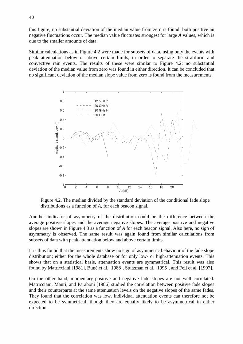
40

this figure, no substantial deviation of the median value from zero is found: both positive annegative fluctuations occur. The median value fluctuates strongest for large A values, which isdue to the smaller amounts of data.

Similar calculations as in Figure 4.2 were made for subsets of data, using only the events withpeak attenuation below or above certain limits, in order to separate the stratiform andconvective rain events. The results of these were similar to Figure 4.2: no substantialdeviation of the median value from zero was found in either direction. It can be concluded thatno significant deviation of the median slope value from zero is found from the measurements.

0 2 4 6 8 10 12 14 16 18 20-1

-0.8

-0.6

-0.4

-0.2

0

0.2

0.4

0.6

0.8

1

A (dB)

med

ian

/ sta

nd. d

ev. (

)

12.5 GHz

20 GHz V

20 GHz H

30 GHz

Figure 4.2. The median divided by the standard deviation of the conditional fade slopedistributions as a function of A, for each beacon signal.

Another indicator of asymmetry of the distribution could be the difference between theaverage positive slopes and the average negative slopes. The average positive and negativeslopes are shown in Figure 4.3 as a function of A for each beacon signal. Also here, no sign ofasymmetry is observed. The same result was again found from similar calculations fromsubsets of data with peak attenuation below and above certain limits.

It is thus found that the measurements show no sign of asymmetric behaviour of the fade slopedistribution; either for the whole database or for only low- or high-attenuation events. Thisshows that on a statistical basis, attenuation events are symmetrical. This result was alsofound by Matricciani [1981], Buné et al. [1988], Stutzman et al. [1995], and Feil et al. [1997].

On the other hand, momentary positive and negative fade slopes are not well correlated.Matricciani, Mauri, and Paraboni [1986] studied the correlation between positive fade slopesand their counterparts at the same attenuation levels on the negative slopes of the same fades.They found that the correlation was low. Individual attenuation events can therefore not beexpected to be symmetrical, though they are equally li kely to be asymmetrical in eitherdirection.

41

0 2 4 6 8 10 12 14 16 18 200

0.05

0.1

0.15

0.2

0.25

A (dB)

aver

age

(dB

/s)

12.5 GHz

0 2 4 6 8 10 12 14 16 18 200

0.05

0.1

0.15

0.2

0.25

A (dB)

aver

age

(dB

/s)

20 GHz V

0 2 4 6 8 10 12 14 16 18 200

0.05

0.1

0.15

0.2

0.25

A (dB)

aver

age

(dB

/s)

20 GHz H

0 2 4 6 8 10 12 14 16 18 200

0.05

0.1

0.15

0.2

0.25

A (dB)

aver

age

(dB

/s)

30 GHz

Figure 4.3. Conditional average positive (- - - -) and negative (−−−) fade slopes for eachbeacon signal.

42

4.2.3. Attenuation dependent distribution model

For the conditional distribution of fade slope ζ for fixed values of attenuation A (shown inFigure 4.1), a model was searched. By trial and error, a reasonable fit was found with thefollowing model distribution:

( )( )( )

p Aζπσ ζ σζ ζ

=+

2

12 2 ((dB/s)-1) (4.2)

This distribution is symmetrical around zero. Its mean value is (consequently) 0 dB/s and theonly characterising parameter is σζ, the standard deviation of ζ. Compared to a Gaussiandistribution with the same standard deviation, the distribution of (4.2) has higher tails and ahigher, sharper peak. In Figure 4.4, the distribution is shown for different values of σζ.

-0.1 -0.08 -0.06 -0.04 -0.02 0 0.02 0.04 0.06 0.08 0.110

-2

10-1

100

101

102

slope (dB/s)

cond

ition

al p

roba

bilit

y de

nsity

(1/

(dB

/s))

sigma = .005

.01

.05

Figure 4.4. Modelled conditional distribution of fade slope ζ, with σζ = 0.005, 0.01,0.015, ..., 0.05 dB/s.

The distribution of ζ for any fixed A value can be modelled by equation (4.2), with σζ as theonly characterising parameter. Comparing Figure 4.4 with Figure 4.1 it can be seen that σζ isdependent on A. To find the relation between these, the value of σζ was calculated from theconditional distribution of ζ for every A-bin, for every beacon signal. In Figure 4.5, the resultsare shown as a function of A. This figure shows that σζ is approximately proportional to A,and that the relation of σζ with A is very similar for all frequencies.

43

0 2 4 6 8 10 12 14 16 18 200

0.05

0.1

0.15

0.2

0.25

A (dB)

stan

d.de

v. (

dB/s

)

12.5 GHz

20 GHz V

20 GHz H

30 GHz

Figure 4.5. σζ as a function of A for each of the beacon signals, and for all beaconstogether (thick dashed line).

The theoretical frequency dependence of the fade slope distribution can be estimated asfollows. According to the ITU-R [1994b], rain attenuation statistics can be scaled in frequencyin the range 7 to 50 GHz by the formula

( )( )A

A

b

b

b b b A2

1

2

1

32 1 1 1

0 551 112 10

=

− × −..

(4.3)

where

bf

fii

i

=+ −

2

4 21 10(4.4)

and f is the frequency in GHz. According to this, the ratio between equiprobable attenuationsA2 and A1 at 30 and 20 GHz is almost constant: with A1 at 20 GHz varying from 1 dB to20 dB, this factor varies from 2.07 to 1.81. Similarly the ratio between equiprobableattenuations at 12.5 and 20 GHz varies from 0.41 to 0.44. This means that the distribution ofA1 at one frequency is almost proportional to that of A2 at another.

Furthermore, since momentary A values at two frequencies are generally found to be very wellcorrelated, also the momentary A1 and A2 are approximately proportional. This property isalready used in many ULPC systems, where the attenuation at one frequency is estimated fromthat at the other [e.g. Sweeney and Bostian, 1999]. We can express this property by a scalingfactor:

A2 = a A1 (4.5)

which is approximately true for each separate sample and for each frequency pair f1 and f2.From equation (4.1) it follows that then also

44

ζ2 = a ζ1 (4.6)

is approximately true for every separate sample. The standard deviation σζ1 of the distributionof ζ1 at f1 conditional for A1 must then also be proportional to σζ2 of the distribution of ζ2 at f2in the same portion of time, i.e. conditional to A2:

σζ2 = a σζ1 (4.7)

In Figure 4.5, σζ was found to be approximately proportional to A for all frequencies:

σζ1 = s1 A1 σζ2 = s2 A2 (4.8)

It follows easily from equations (4.5), (4.7), and (4.8) that the proportionality factors s1 and s2

must be the same. It thus follows that if the conditional fade slope distribution p(ζ|A) isproportional to A, it must be independent of frequency.

This is in agreement with Figures 4.1 and 4.5, where no significant difference between theresults of different frequencies was found. The differences between the curves for high Avalues in Figure 4.5 are due to statistical unreliabilit y because of lack of data. Also Feil ,Ippolito, Helmken, Mayer, Horan, and Henning [1997] observed from measurements from theACTS-satellit e at several ground stations in the US, that the probabilit y of the fade slope at agiven fade level was very similar for 20 and 27 GHz. Of course, the total distributions of fadeslope may still be frequency dependent, due to frequency dependence of the attenuationstatistics.

In order to increase the amount of data per A-bin, the distributions of ζ for all four beaconsignals were put together in one distribution for each bin, and the standard deviations wereagain calculated. The result, as a function of A, is also included in Figure 4.5 (thick dashedline). The result is obviously more stable than the curves for the different beacons, andconfirms that σζ is approximately proportional to A for the analysed data set from the groundstation in Eindhoven. In Section 4.3, this result will be compared to results from othermeasurement sites.

It may be noted that statistics for A = 0 dB are not included in the figures of this section. Thisis because the statistics were generated only over the set of attenuation events. During theremaining non-event period, A can be assumed ≈ 0 dB most of the time, however, noinformation is available about the distribution of the fade slope. The fade slope distributionduring the short pre- and post-event periods with A ≈ 0 dB can not be seen as representativefor the whole non-event time. Therefore, the results from the event-based statistical analysiscannot be used for A = 0 dB.

45

4.2.4. Dependence on rain type

As discussed in Section 4.1, the fade slope depends on wind velocity and drop sizedistribution, and its distribution is therefore likely to be climatic dependent and dependent onthe type of rain. In particular, in a convective rainstorm the rain intensity can be expected tochange suddenly by large steps, while in stratiform rain it varies more gradually, even thoughthe maximum intensity may be equal to that of the convective storm.

It was studied whether this difference in typical behaviour has any effect on the fade slopedistribution, in the following way. The data base was divided in events with peak eventattenuation below certain thresholds, in order to isolate stratiform rain, and above certainthresholds, in order to isolate convective rain. The attenuation at 30 GHz was used in thiscriterion (simply because it was the only copolar beacon which was available during allevents). The dependence of σζ on A was again determined for each data selection; these allagain appeared to be approximately proportional. The coeff icient σζ/A was determined foreach case, and the results are shown in Figure 4.6.

0 2 4 6 8 10 12 14 16 18 204

4.5

5

5.5

6

6.5

7

7.5

8

8.5x 10

-3

B2 peak attenuation below threshold

B2 peak attenuation above threshold

Threshold attenuation (dB)

sigm

a / A

((d

B/s

)/dB

)

Figure 4.6. σζ/A for selections of the database with events with peak attenuation at30 GHz above and below different threshold values.

This figure shows that σζ/A significantly decreases if only the light events are selected, andincreases slightly when only heavy events are selected. (Note that the fluctuations on the leftof the lower curve and on the right of the upper curve are both due to lack of data.) Thismeans that the conditional fade slope standard deviation is smaller for light rain events thanfor heavy rain events, for equal A-values. This is a first indication that the fade slopedistribution is dependent on rain type. No quantitative conclusions can yet be drawn from thisresult, because events of the two rain types were probably not completely separated. It isimpossible to effectively detect stratiform or convective rain using only a peak attenuationthreshold. Nonetheless, this qualitative conclusion is useful when the results of Eindhoven arecompared to those from other sites and climatic dependencies are considered.

46

4.2.5. Dependence on filter bandwidth

Matricciani [1982] performed experiments with fade slope statistics, measured from thesatellit e SIRIO at the ground station of Gera Lario, Italy. The data were sampled at a rate of10 Hz. Scintill ation effects were removed by low-pass filtering the data with two moving-average filters with different time periods: 1 s and 4 s, in order to compare the results. Afterthis, the data were resampled with sampling times equal to the averaging periods. Fade slopewas computed by detecting the time it took the filtered signal to change from certain fixed Avalues to A + ∆A, and from A + ∆A to A. Different values of ∆A were also tested. It appearedthat the results were practically independent of ∆A in the range 1.5 - 3 dB [Matricciani, 1981].

The results using the two different low-pass filters however were significantly different[Matricciani, 1982]. For the total fade slope cumulative distribution (i.e. for all A values),Matricciani found that the results were similar in shape but differed by a scaling factor of theslope. He explained this by the smoothing and resampling which gives rise to longer risingand sinking times over a given ∆A. Furthermore, slopes faster than a certain limit appeared tobe not detected using the 4s-averaging filter. This limit corresponded to a rising/sinking timeof 4s over the distance ∆A.

Also for the conditional distributions for certain A-values Matricciani found a similar scalingeffect. For A = 4.5 dB, the 4s-averaged distribution was similar in shape but for slopes 1.5times lower than the 1s-averaged distribution.

If the same effect is true for other measurements, the results of the previous section shouldalso be dependent on the bandwidth fB of the filter used. This was tested by repeating thestatistical analysis using several filtering bandwidths. For bandwidths from 0.1 mHz to0.2 Hz, distributions of the filtered signal were generated. It resulted that in all cases, theconditional distributions can still be modelled by the distribution of equation (4.2) and Figure4.4, but the values of σζ are significantly different. These are shown versus A in Figure 4.7.This figure shows that for all filtering bandwidths, σζ is approximately proportional to A. Forlarge bandwidths (≥ 0.1 Hz) and low A however, σζ becomes somewhat larger thanproportional to A. This can be explained by scintill ation, which is not filtered out completely.Scintill ation introduces a fade slope distribution which varies less strongly with attenuation(see Section 5.6.1 of this thesis), and therefore has strongest impact for low A-values.

Straight lines with forced zero offset were fitted to the curves of Figure 4.7 (dotted lines in thefigure), using only the parts proportional to A, so that only the effects of rain are included. Theslopes of these lines are plotted in Figure 4.8 versus the filtering bandwidths. It appears thatfor bandwidths down to about 1 mHz, the relation is approximately a straight line in this log-log plot. The deviation for bandwidths below 1 mHz is probably because a too large part ofthe rain attenuation spectrum is cut off . 1 mHz corresponds to an averaging time of 8:20 m:s,which is already longer than some entire rainstorms.

The results indicate that for the measurements in Eindhoven, the fade slope standard deviationσζ can be approximated by

σζ = 0 0298 0 39. .f AB dB/s (4.9)

where fB is the LPF bandwidth (Hz) and is above 0.001 Hz. The coeff icients in this equationcorrespond to the fitted line in Figure 4.8.

47

0 2 4 6 8 10 12 14 16 18 200

0.05

0.1

0.15

0.2

0.25

0.3

A (dB)

sigm

a (d

B/s

)

Figure 4.7. σζ as a function of A using different LPF bandwidths, and zero-offset fittedlines (.......). The bandwidths are, from top to bottom: 0.2; 0.1; 0.05; 0.02; 0.01; 0.005;0.002; 0.001; 0.0005; 0.0002; 0.0001 Hz.

10-4

10-3

10-2

10-1

100

10-3

10-2

filter bandwidth (Hz)

sigm

a / A

(1/

s)

Sharp filtering

Figure 4.8. The slopes σζ/A of the fitted lines in Figure 4.7 versus filter bandwidth (‘*’)and a line fitted in the range ≥1 mHz (........).

As described in the previous section, the filtering method was to rigidly cut off all frequencycomponents above fB. For other types of f ilters, the result may be different. The same analysisas described above was performed for a block-averaging filter, which replaces each block ofdata of a certain length by one sample, equal to the average of the data in this block. Also inthis case, σζ appeared to be approximately proportional to A, and dependent on the length t ofthe averaging blocks. An empirical approximation was found as:

σζ = −0 0164 0 39. .t A dB/s (4.10)

48

for 5 s ≤ t ≤ 200 s. Combining this result with equation (4.9), an effective filter bandwidth ofthe block-averaging filter with block length t is found as

f tB = 0212. (4.11)

If this effective filter bandwidth is used, equation (4.9) can be applied to predict σζ also forblock-averaging filters. The same test was also performed for moving-average filters. Thesefilters replace each sample by the average of the samples in the block of length t around it, butdo not reduce the amount of data. Similarly as for the block-averaging filter, an effective filterbandwidth for moving-average filters was found as

f tB = 0500. (4.12)

for 5 s ≤ t ≤ 500 s. The same test was performed for so-called cos2-filters. This type of f ilter issimilar to a moving-average filter, but before averaging it multiplies the samples in the blockby a cos2-shaped function, with the nulls at the edges and the maximum in the center. Thisaction removes all discontinuities from the signal. From this test, it was found that aneffective filter bandwidth for cos2-filters is given by

f tB = 0 791. (4.13)

for 5 s ≤ t ≤ 500 s.

It can be concluded that the dependence of σζ on filter bandwidth for any LPF filter isexpressed by equation (4.9). For other filters than those with an infinitely sharp edge, theeffective signal bandwidth can be calculated from equations (4.11-13). Equation (4.11) isvalid for block averaged data with block lengths t, which is equivalent to signals sampled withtime resolution t. Equation (4.12) is valid for a moving-average filter, and equation (4.13) fora cos2-filter.

49

4.3. Comparison with other sites

Fade slope has also been measured and analysed at many other experimental sites, and theresults of some of these studies have been published in literature. In this section, some ofthese results are compared to the results from Eindhoven, in order to assess the influence ofother parameters than those discussed in the previous sections.

Statistical results of fade slope are considered only from publications where these are givenspecifically for different attenuation levels. This is because, as was seen above, thedistribution of fade slope depends strongly on the attenuation statistics. Comparison of thetotal distribution between different sites would therefore be very complicated.

Experimental results from 5 sites were found. In Table 4.1, parameters of the measurementsites are given. Some details on the data processing at the different measurement sites aregiven in Appendix A.1. In the publications, the measurement results are usually presented ingraphs. The information has been extracted from these by enlarging the paper copies andscanning the graphs by hand. This way, an estimated accuracy of ≈ 0.1% of the maximumrange of the graphs could be reached.

Table 4.1. Site parameters of the measurements of fade slope distribution: site names,coordinates, frequencies f, elevation angles ε, LPF specifications, satellite names, andreferences.

ground station coord. f(GHz)

ε(º)

LPF satellite reference

Blacksburg,Virginia

37.23 -279.60

12.519.829.7

14 10smov. av.

Olympus Stutzman et al., 1995

Fairbanks,Alaska

64.86 -212.18

20.227.5

8.1 100scos2

ACTS Feil et al., 1997

La Salle,Colorado

40.35 -255.28

20.227.5

43 10smov. av.

ACTS Bringi and Beaver,1997

Tampa, Florida 28.06 -277.58

20.227.5

52.1 100scos2

ACTS Feil et al., 1997

White Sands,New Mexico

32.37 -253.62

20.227.5

51.5 100scos2

ACTS Feil et al., 1997

Unfortunately, it is not possible to compare the shape of the conditional fade slopedistribution, modelled in equation (4.2), with the results from other sites. This is because inthe publications, the fade slope distributions for fixed attenuation levels were not representedin small enough bins to give enough information about the shape of the distributions. It ishowever possible to estimate the standard deviation σζ from the published distributions.

Stutzman et al., and Bringi and Beaver, gave the fade slope ζ (conditional for attenuationlevels) in bins of 0.05 dB/s wide, and Feil et al. in bins of 0.1 dB/s. These bin sizes arerelatively large, especially for small standard deviations (see Figure 4.4), so the distributioncan not be assumed constant within these bins. It would therefore have been too inaccurate toassume e.g. that for all of the measured samples in each bin ζ was exactly at the center of thebin, or homogeneously distributed over the bin. Such an assumption would be necessary if thestandard deviation should be calculated from the distributions directly. However, the standard

50

deviations could be estimated from each bin content as follows. The relation between thestandard deviation σζ and the probabilit y of samples in each bin was calculated using themodel distribution (4.2). By inverting this relation, σζ could be estimated from each bincontent of the measured distributions. This was done for all of the reported conditional fadeslope distributions. In most cases, the resulting σζ was similar for all bins of a distribution,which indicates that equation (4.2) is a good estimate of the measured distributions. The fewoutlying values were removed, and the calculated σζ was averaged over each distribution.

The measurement sites involved in the ACTS-project had a particular problem: a water-absorbing antenna coating which during rain events caused an extra attenuation of up to 3 dBat 20.2 GHz and up to 5 dB at 27.5 GHz [Crane, Wang, Westenhaver, and Vogel, 1997]. Ingeneral, it can be expected that once the antennas had gotten wet, the attenuation caused bythis effect was relatively constant during the rain events. Because of this, the fade slope willnot have been affected very much, but the concurrently measured attenuation was a few dBhigher than that caused by rain alone. In the ACTS-database on the Internet(http://rossby.metr.ou.edu/~actsrain/), correction values are provided to compensateattenuation distributions for this effect. The fade slope distributions used in this study havebeen corrected, by adjusting the A bin values according to these correction values.

Comparing the results from all of the sites, it appeared that the values of σζ were notsignificantly different for different frequencies, similarly as found from the Eindhoven results.This confirms once more that σζ does not depend on frequency. The resulting values from thedifferent frequencies were averaged for each A-value.

As was found in the previous section, σζ depends strongly on the filtering used before thedistributions are generated. In order to compare the different results, the values of σζ werenormalised by dividing them by fB

0.39, where fB is the LPF bandwidth, which was estimatedusing equations (4.11)-(4.12), depending on the type of filter.

In Figure 4.9, the normalised standard deviations from all of the reported sites are plotted asfunctions of A. This figure shows, that although for all sites σζ increases with A, somesignificant differences remain.

Figure 4.9 shows that for each station, the normalised σζ can be approximated as proportionalto A:

σζ ≈ s f AB0 39. dB/s (4.14)

The value of the coeff icient s was determined for each station by fitting zero-offset straightlines to the curves of Figure 4.9. The results of this are:

s ( )Eindhoven 0.015Fairbanks 0.021Blacksburg 0.020White Sands 0.040Tampa 0.046La Salle 0.056

51

0 2 4 6 8 10 12 14 16 18 200

0.1

0.2

0.3

0.4

0.5

0.6

Fai

Bla

Ein

Whi

Tam

LaS

A (dB)

norm

alis

ed s

igm

a (d

B/s

)

Figure 4.9. Normalised σζ as a function of A for la Salle, Tampa, White Sands,Blacksburg, Fairbanks, and Eindhoven (each one indicated by the first three letters ofthe name).

Feil et al. explained the different result from Fairbanks from those from Tampa and WhiteSands by suggesting that the fade slope distribution is dependent on elevation angle. Thisseems plausible, considering that lower elevation links have a longer path length through rain.As discussed in Section 4.1, a certain attenuation level on a longer path, being more likelycaused by widespread rain or several rain cells, is less likely to change rapidly than the sameattenuation on a shorter path, more likely caused by a single rain cell . A parameter expressingthe influence of the elevation angle ε by the expected dependence on path length is sin(ε),which is proportional to the path length through rain (if the rain height is constant). In Figure4.10, the parameter s is shown for all sites versus sin ε.

In Figure 4.10, some of the results indeed seem to indicate an elevation dependence: σζ inFairbanks, Blacksburg, and Eindhoven is lower than in la Salle, White Sands, and Tampa. Onthe other hand, in Eindhoven σζ is lower than in Fairbanks, and in la Salle higher than inTampa. This indicates that there must be other influencing parameters than the elevationangle.

52

0 0.1 0.2 0.3 0.4 0.5 0.6 0.7 0.8 0.90.01

0.015

0.02

0.025

0.03

0.035

0.04

0.045

0.05

0.055

sin (elevation)

s (

)

FaiBla

Ein

Whi

Tam

LaS

Figure 4.10. The correlation of the parameter s with sin ε.

Feil et al. found that their results from Tampa and White Sands were similar although comingfrom very different climatic regions (and similar elevation angles). They therefore concludedthat fade slope is not correlated with climatic region. Still , climatic differences might explainthe differences between the other results in Figure 4.9. In Section 4.1, it was discussed that,because of the influence of drop size distribution and wind velocity, the distribution of fadeslope may be climate dependent. In order to find a climatological explanation of thedifferences, the climatic characteristics of the measurement sites, according to the Köppenclassification, are reviewed below [Lutgens and Tarbuck, 1998]. The main characteristics aresummarised in Table 4.2.

Table 4.2. Climatic characteristics according to the Köppen classification(T is the average temperature).

site(s) climate general winters summersWhite Sands Subtropical

Steppedry; semi-arid cool; dry

T ≈ 0ºCwarm; dryT > 22ºC

La Salle Middle-LatitudeSteppe

little, unreliableprecipitation

cold; dryT ≈ 0ºC

warm; occasionalrain; T > 22ºC

Tampa;Blacksburg

HumidSubtropical

rainy;constantly moist

mild; wet0º < T < 18ºC

warm; wetT > 22ºC

Eindhoven MarineWest Coast

rainy; variable;constantly moist

mild; wet0º < T < 18ºC

cool; wet10º < T < 22ºC

Fairbanks Subarctic cold; dry; stable severe; dryT < 0ºC

cool; quite dry; short10º < T < 22ºC

The Subtropical Steppe is a semi-arid area surrounding an arid desert area, and governed bya pronouncedly dry climate. This is a consequence of the subsidence and market stabilit y ofthe subtropical highs around the Tropics of Cancer and Capricorn. In some steppe areasrelatively far from the equator (including possibly New Mexico), the rare precipitationconcentrates in the winter, when middle-latitude cyclones take more equatorward routes andbring occasional periods of rain. The rain is typically a harsh downpour of very short duration[Feil et al., 1997].

53

The Middle-Latitude Steppe such as in North America is, unlike its subtropical counterpart,kept dry not by subtropical highs but by being far away from the oceans and shielded by highmountain ranges. In winter, high pressure and cold temperatures dominate the continent,opposing precipitation. In summer, the subtropical anticyclone disappears over the continentand higher surface temperatures and greater mixing ratios prevail , conducing somewhat morecloud formation and precipitation.

The Humid Subtropical climate resembles in the summer the rainy tropics: hot, humid, andwith convectional showers and thunderstorms in the afternoon or evening. These are due towarm, moist air that moves in from the oceanic subtropical anticyclone over the heatedcontinent and becomes increasingly unstable there. Winters are different: winter precipitationis widespread rain and snow, generated along fronts of the frequent middle-latitude cyclones.The Humid Subtropical climate covers the whole North-American south/east coast. Summertemperatures are similar over this area, but the winter temperatures vary strongly with latitude.The monthly average temperature in January is about 16ºC in Florida and 3º in Virginia.

The Marine West Coast climate is dominated by the onshore flow of oceanic air, causingmild winters, cool summers, and ample rainfall throughout the year. In some places on theglobe, this climatic zone occurs as a narrow strip between the coast and a mountain rangewhich blocks the marine air, causing it to lose much water before moving further inland.However, in central Europe no such mountain barrier exists, and widespread rain falls fromfreely inland moving air. Due to this, in the Netherlands, rain usually coincides with westerlywind.

In the Subarctic climate in Alaska and interior Canada, winter dominates: it is long andbitterly cold. The summers are relatively warm, even though cool compared to regions farthersouth. Annual temperature ranges in Subarctic climate are the largest on earth. The conditionsare stable all year through, and are not influenced by air moving in from any other region. Dueto this, and because of the limited moisture capacity of the cool air, precipitation amounts aresmall . Most of it comes as rain from scattered summer convectional showers. In this area, colddry air masses are formed which can move southward and influence the weather in otherregions.

With this information, some of the differences in the results of Figure 4.9 can be explained. InEindhoven, rain is usually of the widespread type, while in la Salle, White Sands and Tampaconvective rain prevails. This suggests that convective rain causes higher fade slopes thanwidespread rain for similar attenuation values, which is in agreement with the conclusion ofSection 4.2.4. Also in Fairbanks the rare rain is usually convective, but the normalised σζ isrelatively low. This may be due to the low elevation angle, which indicates that the elevationangle also has some influence. Blacksburg is, according to Köppen, in the same climatologicalregion as Tampa, but its normalised σζ is lower. This can be due both to the lower elevationangle and to the more northerly location, causing the site to experience more middle-latitudecyclone fronts with widespread rain than Tampa.

A meteorological parameter which expresses the prevalence of convective rain was providedby J. Pedro V. Poiares Baptista of ESTEC. This parameter cr, the convectivity of rain,represents the average amount of convective rainy time relative to the total rainy time. It wasgiven in a global matrix with a spatial resolution of 1.5º both in latitude and longitude. Thevalue of cr for the sites considered here was calculated by two-dimensional li near interpolationbetween the four nearest grid points. The results of this are:

54

cr ( )Eindhoven 0.175Fairbanks 0.219Blacksburg 0.355White Sands 0.471Tampa 0.650La Salle 0.397

In Figure 4.11, the parameter s is shown versus the rain convectivity cr. This figure showsthat, similarly as with sin ε, there is a significant correlation in some, but not in all cases. Inparticular, in la Salle s is much larger than in Blacksburg, while cr is almost equal in those twoplaces.

0.1 0.2 0.3 0.4 0.5 0.6 0.70.01

0.015

0.02

0.025

0.03

0.035

0.04

0.045

0.05

0.055

convectivity ( )

s (

)

FaiBla

Ein

Whi

Tam

LaS

Figure 4.11. The correlation of the parameter s with the convectivity of rain cr.

Since both parameters sin ε and cr show partially a good correlation with s, it might beexpected that using a combination of the two, all differences between the results may beexplained and a global prediction model of the fade slope distribution may be developed.Unfortunately, this appears not possible. In Figure 4.10 was seen that in Eindhoven, s islowest of all , while sin ε is higher than in Fairbanks and Blacksburg. This could be explainedby cr, which is lowest in Eindhoven. On the other hand, the difference in s between La Salleand Blacksburg while cr is similar, could be explained by their difference in ε. Theseobservations thus point in different directions with respect to the relative importance of thetwo parameters sin ε and cr. Finally, in La Salle, s is highest of all while both ε and cr arelower than in Tampa and White Sands.

It can thus be concluded that s is probably dependent on ε, and on cr or another parameterexpressing the convectivity of rain, but the exact form of this dependence remains as yetunclear. s is lowest in the Subarctic and Marine West Coast climates, and highest inSubtropical climates.

55

4.4. Conclusions

The long-term probabilit y distribution of fade slope ζ, for a certain value of attenuation, issimilar for positive and negative fade slopes, independent of frequency, but dependent onfilter bandwidth. For a fixed link it only depends on rain type and attenuation level. Theconditional distribution can be approximated by

( )( )( )

p Aζπσ ζ σζ ζ

=+

2

12 2 ((dB/s)-1) (4.2)

The only parameter of this distribution is the standard deviation σζ, which for a given link isapproximately proportional to attenuation A. It can be approximated by

σζ ≈ s f AB0 39. dB/s (4.14)

where fB is the filter bandwidth. The coeff icient s is independent of frequency, but differs fordifferent rain types and also between different sites. It may be dependent on elevation angle,and is certainly dependent on climate. Results from several sites indicate that s is lowest forthe Subarctic and Marine West Coast climates, and highest for Steppe and Humid Subtropicalclimates.

The results obtained in this chapter are important steps to the development of an accuratemodel to predict fade slope statistics from attenuation statistics. This information is essentialto assess the minimum speed with which an ALC system should be able to follow changes inrain attenuation.

56

57

5. Scintillation

5.1. Introduction

This chapter describes the results of a study on tropospheric scintill ation on satellit e links thathas been performed at Helsinki University of Technology, (‘HUT’) under ESA/ESTECcontract. The major objectives of the study were:• to obtain statistics of scintill ation from the 20 and 30 GHz Olympus measurements on a

12.7° elevation path• to improve or develop models for scintillation predictions• to develop methods to combine scintillation and attenuation to predict the total fade margin• to obtain relevant meteorological data for scintillation and attenuation studies.

The results of this study are extensively described in the report of the contract study [van deKamp, Tervonen, Salonen and Kalli ola, 1997]. In this chapter, the results concerning differentaspects of scintill ation relevant to Adaptive Link Control systems, as discussed inSection 2.4.1, are presented. These aspects are statistical properties, frequency scaling relationand prediction from meteorological information. The results are presented in the followingsections as summarised below.

In Section 5.2, the existing theory and prediction models of tropospheric scintill ation arereviewed. Also some new theoretical analyses are presented, which can contribute to thedevelopment of new prediction models.

In Section 5.3, a statistical analysis of the measured data is presented. Distributions of signalvariance and of signal level are generated. The distributions are compared to theoreticaldistributions and to the existing prediction models. The signal level distributions are alsocompared to results from other measurement sites. Where necessary, new prediction modelsfor the statistical properties of scintillation are derived.

In Section 5.4, the frequency dependence of scintill ation is studied using the measuredcorrelation of scintill ation variances at 20 GHz and 30 GHz. The frequency scaling ratio iscalculated from this distribution, and the result is compared to the theoretical ratios, and toresults from other measurement sites. Theoretically, scintill ation is expected to be independentof polarisation angle; this is verified by means of a joint analysis of the standard deviations of20 GHz at horizontal and vertical polarisation.

In Section 5.5, the relation of scintill ation with meteorological parameters is studied.According to existing prediction models, there is a long-term correlation (averaging time ≥ 1month) between the scintill ation variance and the wet term of surface refractivity. Thisrelation is verified using the measured data. It is also studied whether there is any correlationwith other meteorological parameters, such as cloud information, both on a long and a shorttime base. For this purpose, statistics of the variances of the data are presented as a function ofthe hour of the day. For the test of the long-term correlation with meteorological parameters,measurement results from different sites are compared.

In Section 5.6, the relation between scintill ation and attenuation is studied by generating jointdistributions of scintill ation variance and mean attenuation from the data. The influence ofthis relation on the total fade statistics (scintillation + attenuation) is examined.

58

5.2. Theory of tropospheric scintillation

5.2.1. Wave propagation in the turbulent atmosphere

The basis for the theory of scintill ation is the fluid dynamics model for velocity fluctuations ina turbulent medium, proposed first by Kolmogorov. Two scales of turbulence can beidentified: the outer scale l1 and the inner scale l2. If kinetic energy is introduced into a fluid atsome large scale l1 (the input range), it results in a turbulent flow. At that large scale, thedissipation is negligible and the energy is transferred successively into eddies of decreasingsize (the inertial range). The relation between velocity fluctuations and eddy sizes followsfrom energy considerations. Finally, a scale size l2 is reached, where the production rate anddissipation rate are of the same order, and the energy is transferred into heat (dissipationrange).

The inner scale l2 is in the order of a millimetre, while the outer scale l1 ranges from a fewtens of meters to a kilometre. It is assumed that at any size between the inner and outer scales(the inertial subrange), the eddies are isotropic. Furthermore, in the lower atmosphere l1 isgenerally assumed to be of the order h⁄3, where h is the height [Fante, 1980].

Temperature, pressure and humidity variations result in refractive index variations. To this,the theory of velocity variations was applied by Tatarski [1961], in order to derive an estimateof signal fluctuations. This theory eventually leads to the von Karman representation of thespatial spectrum of refractive index fluctuations [Ishimaru, 1978]. The structure constant Cn

2

of refractive index fluctuations, which is the main characterising parameter of the modelsderived from Tatarski's theory, is a measure of the spatial variance of the refractive indexfluctuations. It is dependent on height, which is important for elevated propagation paths.When the size of the eddies becomes larger than the size of the first Fresnel zone, theircontribution to the signal fluctuation decreases.

The fluctuations in amplitude of the received signal due to refractive index variations aregenerally expressed in terms of the amplitude deviation from the mean signal amplitude,expressed in dB. For a homogeneous turbulent path of length L, and assuming a pointreceiver, the variance σy

2 of the log-amplitude variation y is given by:

σy n2 2 7 6 11 62316= . C k L (5.1)

where k is the radio wave number = 2πf c with c the velocity of light, and for l2 < λL << l1,which is valid for the microwave region. For sizes outside this inertial subrange, otherexpressions were derived [Tatarski, 1961; Cole, Ho and Mavrokoukoulakis, 1978]. For aninhomogeneous propagation path, Cn

2 needs to be integrated along the path.

For an antenna of diameter D, some correction to equation (5.1) is necessary to account for thefact that as the antenna diameter increases the incident wave front fluctuations become lesscorrelated across the aperture. As the antenna output is a spatial integral of the variousincident rays, the antenna acts as a low-pass filter for the scattered components correspondingto wavelengths smaller than about D. Hence, the observed signal fluctuations are smaller thanthose obtained from a point antenna. This subject has been covered by various authors. Usinga simplified model for the antenna pattern, Haddon and Vilar [1986] found that the aperturesmoothing factor is given by

59

( ) ( )g D xx

x

x x

e

for

= +

−

≈ − <<

38637 111

6

17 0835

1 70835 1

2 1112 5 6

5 6

. sin arctan .

.

(5.2)

where x = 0.0584kDe2/z is a measure of the ratio between the effective antenna diameter De

and the Fresnel zone size 2πz k , with z = the distance of the turbulent layer from the

receiver. De can be calculated from the geometrical antenna diameter D and the antennaaperture efficiency η, as

De = D η (5.3)

The distance z of the turbulent layer can be calculated from the height h of the layer as:

zh

h a=

+ +2

22sin sinε εe

(5.4)

where ε = the elevation angle and ae is the effective radius of the earth including refraction,which is dependent on station height, and at sea level becomes 8.5×106m.

5.2.2. Short-term signal fluctuations

It is generally assumed, that the signal level fluctuations due to turbulence on a short-termbasis (i.e. up to several minutes) show a Gaussian distribution around the mean signal level.This is why they are often characterised only by the variance σ2, as in Section 5.2.1. Underthis assumption, the probabilit y density function of signal deviation y from the mean signallevel can be written as

( )p y y= −1

222 2

σ πσe (5.5)

Some indications of a different short-term behaviour have also been found. As an example,Banjo and Vilar [1986] found that for the largest scintill ation intensities, the short-termdistribution function shows a negative skewness, and thus significantly departs fromGaussian. It appears that the negative signal deviations, generally referred to as ‘f ade’ , are onaverage larger than the positive signal deviations, generally referred to as ‘enhancement’ ,especially for large signal fluctuations. This behaviour is not predicted using a Gaussiandistribution.

The physical background for the Gaussian pdf of signal fluctuations in dB lies in a certainmodelli ng approach. Strohbehn, Wang and Speck [1975] pointed this out for optical signalsscattered by a random medium. If the receiver is located inside the turbulent medium, and thescattering volume is long and narrow, the received field is a result of multiple scattering.Since the received field E is then the product of the incident field multiplied by a number ofindependent factors, the application of the central-limit theorem to log E leads to a (complex)Gaussian distribution for log E, a Gaussian distribution for y ~ Re (log E) = log |E|, and a log-normal distribution for |E|.

However, the main cause of scintill ation on a satellit e link is turbulence in clouds [van deKamp, Tervonen, Salonen, and Poiares Baptista, 1999]. This implies that the turbulent layer is

60

likely to be a thin layer far from the receiver. In this configuration, the received field is thesum of a large number of waves scattered from different regions in the slab with uncorrelateddielectric constants. The received field E can be written as

( )E E j ft x t= +12e π ~ (5.6)

where E1 = amplitude of the direct (unrefracted) wavet = time

( )~x t = a stationary random complex signal, with a narrow spectrum centered at f.

Applying the central-limit theorem in this situation leads to the conclusion that ( )~x t is a zero-mean Gaussian process. Resulting from this approach, the received electric field amplitudeE0 = |E| will not follow a log-normal, but a Rice-Nakagami distribution:

( )p EE

E E

IE E

002

02

12

2

00 1

2

2=

+

σσ

σx

x

x

e

-

(5.7)

where σx = standard deviation of ( )~x t

I0( ) = modified Bessel function of 0th order.

For very small standard deviations, the difference between the lognormal and the Rice-Nakagami distributions is small. However, as the standard deviation becomes moderate orlarge, the difference becomes easily recognisable. Lawrence and Strohbehn [1970] gave anreview of experimental results and considerations made until 1970, favouring each of thesedistributions. Although no well-accepted decision for either of the two had ever been made, aGaussian distribution for y has generally been assumed from that time onwards.

Now, the distribution function of signal level y in dB according to the latter approach will bederived [van de Kamp, 1998]. It may be assumed that the interfering multipath signal,originating from refraction on the turbulent eddies, is proportional to the direct signalamplitude E1. Under this assumption, σx will be proportional to E1:

σx = ξ E1 (5.8)

The signal deviation from the mean on a dB-scale can be calculated from:

yE

E=

20 0

1

log (5.9)

The distribution of y is then given by:

( ) ( ) ( )p ydE

dyp E E y p E= = =0

0 1 0

10

2010 20ln

=− +

ln 10

20

102 20 102 20 1 2 10 20

12

2

12 2

01

2

2E

y E y

IE y

σ

σ

σx

x

x

e (5.10)

61

and with (5.8):

( )p yy

y

Iy

=+

ln 10

20

102 20 102 20 1 210 20

2

2

0 2ξ

ξ

ξe-

(5.11)

Thus, the only parameter influencing this distribution is ξ = σx/E1, which is a measure of theintensity of the scintillation. Figure 5.1 shows the distribution p(y) for various values of ξ. It isclearly seen that as ξ increases, not only the spread increases (generally measured as thestandard deviation σy or the variance σy

2), but also the skewness of the distribution.

The distributions in Figure 5.1 have been plotted as a function of the signal level deviationfrom the mean. So, by definition, the mean value of all distributions in the figure is 0 dB.

-20 -15 -10 -5 0 5 100

0.1

0.2

0.3

0.4

0.5

0.6

0.7

0.8

0.9

1

y (dB)

Pro

babi

lity

dens

ity (

1/dB

)

Figure 5.1. Probability density distribution of signal level y (in dB), for values of theparameter ξ = 0.05 (sharpest peak), 0.1, 0.15, ..., 0.4 (largest spread).

Even though this skewing effect has often been observed [e.g. Banjo and Vilar, 1986; Otungand Evans, 1995], the short-term signal level distribution p(y) is still mostly modelled asGaussian, and in many projects (among which the one described in this chapter), the variance

σ2 or the standard deviation σ σ= 2 over a period in the order of 1 minute is taken as theonly characterising quantity of signal fluctuations due to scintill ation. The relation of thesequantities with ξ is demonstrated in Figure 5.2, where the standard deviation σy of y, ascalculated numerically from the distributions p(y), is shown as a function of ξ.

62

0 0.05 0.1 0.15 0.2 0.25 0.3 0.35 0.4 0.45 0.50

0.5

1

1.5

2

2.5

3

3.5

4

parameter ksi ()

sigm

a_y

(dB

)

Figure 5.2. Standard deviation of signal level in dB, σy, versus the parameter ξ.

5.2.3. Distribution of standard deviation

The scintill ation standard deviation σ shows on a long-term basis (i.e. from several weeks)some variations, which are not Gaussian distributed. Moulsley and Vilar [1982] found a goodfit of the distribution of the standard deviation with a lognormal distribution. This can beexpressed as [Ortgies, 1985]:

( )

( )p

m

σπ σ σ

σσ=

−−

1

10 22

2

2

ln

log

l

l

le (5.12)

where log = the 10-based logarithmln = the e-based logarithmml = the mean value of log σ;σl = the standard deviation of log σ(with σ in dB).

This means that log σ is normally distributed, and therefore also log(σ2) = 2 log σ must benormally distributed. So, also the variance will then satisfy a lognormal distribution:

( )( )

p

m

σπ σ σ

σσ2

2

2 2

21

10 22=

−−

ln

log

l2

l2

l2e (5.13)

where ml2 = the mean of log σ2 = 2ml;σl2 = the standard deviation of log σ2 = 2σl.

Karasawa, Yamada and Allnutt [1988], however, claim that the long-term distributionfunction of the standard deviation can be closely approximated by a Gamma distribution:

63

( ) ( )( )

pa m

aa m

a

aσ σ σσ σ= −−

Γ1 e (5.14)

where a = mσ2/σσ

2;mσ = the mean value of σ;σσ = the standard deviation of σ;Γ( ) = the Gamma function, defined as:

( )Γ a x dxa x= − −∞

∫ 1

0

e (5.15)

The distribution function for the scintillation variance would then be:

( ) ( ) ( )( ) ( )p

p a m

aa m

aa

σσσ

σ σσ σ2 2 2 12

2 2= = −−

Γe (5.16)

This is not a Gamma distribution itself. It is further stated by Karasawa et al. that the relation

mσ σσ2 210= (5.17)

is satisfied. This indicates that the Gamma distribution is determined by only one parameter.

In this study, the measured distributions of scintill ation variance will be compared to both ofthese models, for different time ranges and for the different frequencies. The presumedrelation between mσ and σσ of equation (5.17) will also be verified.

64

5.2.4. Prediction models

5.2.4.1. Models for long-term standard deviation

The derivation of a prediction model for long-term scintill ation standard deviation directlyfrom the theory of Section 5.2.1 would impose a diff iculty: the structure parameter of therefractive index variations Cn

2 is an essential atmospheric parameter e.g. in equation (5.1), butthis parameter can not directly be measured. Thus, some quantification must be obtained fromscintill ation measurements, and the model can be further developed semi-empirically, usingthe various other dependencies derived from theory. This has been done by variousresearchers.

Rogers and Allnutt [1987] showed, that Tatarski's formulation predicts that the standarddeviation σ, of the amplitude fluctuations in log-power, depends upon frequency, elevationangle and antenna size, as:

( )σ ε∝ g D fe7 12 11 12sin / (5.18)

where f is the frequency in GHz, ε is the apparent elevation angle, and the antenna averagingfunction g(De) is given by:

( )g D

D

z

D

zD

z

D

zD

z

2

10 0 7 0 10

0 5 0 2 10 2 0

01 2 0

e

e e

e e

e

for

for

for

=

−

≤ ≤

−

< ≤

<

. . .

. . . .

. .

λ λ

λ λ

λ

(5.19)

where λ is the wavelength in m, De is the effective antenna diameter, given in equation (5.3),and z is the distance of the turbulent part of the path, given in equation (5.4). This alternativeto equation (5.2) is a piecewise linear approximation of the antenna averaging function fromTatarski [1961]. The scaling of equation (5.19) was, according to Rogers and Allnutt,“ thought to be acceptably accurate for frequencies of 1 to 35 GHz and practical antennadiameters. Application for path elevation angles below about 3° is not recommended becauseof the severe atmospheric multipath that can occur at very low angles.”

Karasawa, Yamada and Allnutt [1988] presented a prediction method for the calculation ofthe standard deviation of signal fluctuations due to scintill ation, starting with equation (5.1),for an inhomogeneous path (Cn

2 height dependent). They performed measurements during theyear 1983 at Yamaguchi, Japan, at an elevation angle of 6.5°, frequencies of 11.5 and14.2 GHz and an antenna diameter of 7.6 m. For the elevation angle dependence, they usedlong-term data from the same site, at elevation angles of 4° and 9°. An empirical estimation ofthe intensity of the fluctuations, equivalent to giving a Cn

2 profile, is represented by thenormalised prediction σn, which is a function of ground refractivity.

The resulting prediction has the form

( )σ σ ε= 0 0228 0 45 1 3. sin. .n ef g D (5.20)

65

where

σ n wet= + × −015 52 10 3. . N dB (5.21)

( )

( )N

RHT T

Twet

e=+

+22790

197 273

2732

.(5.22)

and g(De) is given by equation (5.19), Nwet is the wet term of the refractivity at ground level,RH is the relative humidity in %, and T is the temperature in °C. For the calculation of z in(5.19), Karasawa et al. suggest a value for the height h of the (thin) turbulent layer of 2000 m.For elevation angles below 5º, sin ε in equation (5.20) should be replaced by

( )sin sinε ε+ +2 2 2h aw e , where hw is the effective height of water vapour in the

atmosphere, also assumed 2000 m, and ae is the effective earth radius.

The Karasawa model was tested against measurements from four different sites in WesternJapan, and from Haystack (USA) and Chilbolton (UK). These measurements were made atelevation angles from 4° to 30°, frequencies from 7.3 to 14.2 GHz, and with antennadiameters from 3 to 36.6 m. The average Nwet in these different databases varied from 20 to130 ppm. Karasawa et al. mention that the model is expected to be applicable to world-wideregions with different meteorological conditions, but state that to verify or improve theprediction procedure, a collection of data at lower elevation angles and from different climaticregions is required.

ITU-R Recommendation PN. 618-3 [1994b] contains another model. Following the basicformulation technique employed in the Karasawa model, they present the following predictionformula:

( )σ σ ε= n ef g D7 12 1 2sin . (5.23)

where

σ n wet= × +− −36 10 103 4. N dB (5.24)

and g(De) is the aperture averaging function of Haddon and Vilar, given in equation (5.2). Avalue of the height h of the turbulent layer of 1000 m is suggested by ITU-R.

This model is based upon measurements covering elevation angles in the range of 4° to 32°,antenna diameters between 3 and 36 m, a frequency range of 7 to 14 GHz and severaldifferent climatic regions.

Both of these models are applicable to meteorological measurements averaged over a periodin the order of a month. Short-term scintill ation, varying with daily weather changes, can notbe predicted with these, as is stated in the respective documents. It would be interesting to seewhich is the minimum period over which should be averaged, to apply the models. Thisquestion will be addressed in Section 5.5.1.

None of the frequencies used in the HUT project lie in the range for which these models havebeen validated. It is therefore useful to compare both of these models to the measurement

66

results, so they can, if necessary, be adjusted to fit in a wider frequency range. This will bedone in Sections 5.4.1 and 5.5.

A very uncertain parameter in the testing and application of both the Karasawa and ITU-Rmodels seems to be the height h of the turbulent layer. Some estimations of this quantity canbe made using some meteorological measurements as the height profiles of temperature andhumidity, or spectral analysis of scintill ation measurements, but still very littl e is known withcertainty about it. However, it needs to be said that, for the measurements of the Olympussignals at Kirkkonummi, the models do not depend very strongly on the value of h. This canbe quantified as follows: the effective antenna diameter at Kirkkonummi is 1.43 m at 20 GHzand 1.11 m at 30 GHz, and the elevation angle of Olympus is 12.7º. Then if h varies from 500to 5000 m, the aperture smoothing factor g2(De) of equation (5.2) varies from 0.857 to 0.972for 20 GHz and from 0.866 to 0.974 for 30 GHz. The antenna averaging factor g2(De) ofequation (5.19) varies in this case from 0.830 to 0.946 for 20 GHz and from 0.838 to 0.949 for30 GHz. A stronger dependence may be expected for a larger antenna or a larger elevationangle.

5.2.4.2. Models for signal level distribution

The development of models predicting the long-term distribution of signal level deviation dueto scintill ation has, in general, also taken place semi-empirically. Theoretically, an estimationof this distribution can be calculated from the distribution of short-term signal standarddeviations using the equation:

( ) ( ) ( )p y p p y d=∞

∫ σ σ σ0

(5.25)

where p(σ) is the distribution function of short-term standard deviations σ, and p(yσ) is theshort-term distribution function of signal level y for a given standard deviation. This formulais correct if it can be assumed that the distribution function p(yσ) is only dependent on thevalue of σ.

For p(yσ), the Gaussian distribution of equation (5.5) can be written, or the alternativedistribution of equation (5.11). Equation (5.25) can then be used to calculate from adistribution p(σ) of short-term standard deviations, the long-term distribution of signal leveldeviation. Ortgies [1985] has shown this method to give reasonable results, using a Gaussiandistribution for p(yσ), even though this way the asymmetry between signal enhancement andfade is ignored.

Karasawa, Yamada and Allnutt [1988] present some expressions for the long-term cumulativedistribution of amplitude deviation y, expressed in terms of the predicted long-term standarddeviation. This has been derived from equation (5.25) with a Gaussian distribution assumedfor p(y|σ) and a Gamma distribution for p(σ). Also, the relation in equation (5.17) wasassumed between the long-term mean and standard deviation of σ. The resulting amplitudedeviation, exceeded for a time percentage of P, is given by:

( )y P P P= − − − +00597 00835 1258 26723 2. log . log . log . σlt (5.26)

(0.01% ≤ P ≤ 50%)

67

where σlt is the long-term signal standard deviation, which can be calculated from equation(5.20). Equation (5.26) agreed well with the measurements of Karasawa et al. for signalenhancement. For signal fade however, the measured deviation was larger, especially in thelow probability region. They fitted a curve to these measurement results, giving the relation:

( )y P P P= − + − +0061 0072 171 303 2. log . log . log . σlt (5.27)

(0.01% ≤ P ≤ 50%)

The ITU-R adopted only the distribution (5.27) for signal fade in their proposed predictionmethod.

These two expressions are plotted in Figure 5.3, for a normalised signal deviation y/σ.

0 1 2 3 4 5 6 7 810

-2

10-1

100

101

102

y / st.dev. ()

cum

ul. p

roba

bilit

y (%

)

fade

enhancement

Figure 5.3. Cumulative probability of normalised signal enhancement and fadeaccording to Karasawa et al.

It appears that the long-term cumulative distribution, when expressed as y(P), is proportionalto σ. This results from the theoretical calculation using a Gamma distribution for p(σ), underthe assumption that σσ and mσ are proportional, as in equation (5.17). If this condition is notsatisfied, the dependence of y(P) on σ becomes more complicated.

The difference between fade and enhancement is due to the asymmetry of short-term signallevel fluctuation, which was described in Section 5.2.2. This asymmetry is not accounted for ifa Gaussian distribution is assumed for p(yσ). However, Figure 5.1 shows that thedistribution of equation (5.11), which assumes a Rice-Nakagami distribution for the receivedelectric field amplitude, does show a different behaviour for signal fade and enhancement.This has been used to derive a theoretical expression for the long-term distribution of signallevel taking into account the asymmetry of the fluctuations [van de Kamp, 1998]. For this, thedistribution of equation (5.11) has been substituted for p(yσ) in equation (5.25). Equation(5.11) expresses this distribution as dependent on ξ, and the relation between ξ and σ is found

68

from Figure 5.2. Similarly as done by Karasawa et al., the Gamma distribution (5.14) wastaken for p(σ), and the assumed relation (5.17) between mσ and σσ was used. The result of thisintegration is shown in Figure 5.4, for a normalised signal deviation y/mσ, and for differentvalues of mσ.

0 1 2 3 4 5 6 7 8 9 1010

-3

10-2

10-1

100

101

102

y / st.dev. ()

cum

ul. p

roba

bilit

y (%

)

0.20.4

0.60.8

1.00.2 0.4 0.6 0.8

1.0

fade

enhancement

Figure 5.4. Cumulative distribution of normalised signal enhancement and fade,calculated using the distribution of equation (5.11), for indicated values of mσ (dB), andthe model by Karasawa (dotted line).

In this figure, the difference between signal fade and enhancement clearly appears. Thisdifference significantly increases with increasing mean standard deviation mσ: the normalisedenhancement decreases and the normalised fade increases with mσ for fixed exceedanceprobabiliti es. The Karasawa model does not account for this dependence. The observeddependencies can be modelled as follows. If the cumulative distribution of signal fade isindicated as yf(P) and of signal enhancement as ye(P), these distributions can be written as

yf(P) = γ(P) + δ(P) (5.28a)

ye(P) = γ(P) − δ(P) (5.28b)

In Figure 5.4, it appears that γ(P) can be approximated by Karasawa’s expression (5.26),which is the theoretical result if the skewness of the short-term distribution is ignored:

γ(P) = (−0.0597 log3P − 0.0835 log2P − 1.258 log P + 2.672) mσ (5.29)

δ(P) can be approximated by:

δ(P) = (0.100 log2P − 0.375 log P + 0.297) mσ2 (5.30)

The goodness of agreement of these expressions with the distributions resulting from theintegrations can be expressed as follows: the relative error in signal fade or enhancement is

69

smaller than 10% for 0.001% ≤ P < 50% and 0.2 dB ≤ mσ ≤ 1 dB. The absolute error forsignal enhancement is smaller than 0.25 dB over the same ranges; for fade it is smaller than0.25 dB for 0.2 dB ≤ mσ ≤ 0.8 dB and smaller than 1.0 dB for 0.2 dB ≤ mσ ≤ 1 dB.

Apparently, the average of the normalised fade and enhancement distributions isapproximately equal to the enhancement distribution according to Karasawa. This and thedependence on the long-term standard deviation are the main differences with the Karasawamodel. In Section 5.3.2.1, the Karasawa model will be compared to measurement results. Theproperties found from the theoretical analysis of this section will be used to explaindifferences between the Karasawa model and measurements, and to develop an improvedprediction model.

70

5.3. Statistical measurement results from Kirkkonummi

In this and the following sections, the main results will be presented of the scintill ationanalysis, performed at Helsinki University of Technology (HUT) using beacon measurementsreceived from the Olympus satellit e. The Olympus propagation experiment and themeasurement set-up at HUT are described in Sections 3.1-3.2.

5.3.1. Distribution of variance

In Figures 5.5 and 5.6, the probabilit y density functions of variance of 20 GHz V and30 GHz V, over the year 1990 (Data Set 1), are shown. Distributions for each separate monthwere also generated [van de Kamp, Tervonen, Salonen, and Kalliola, 1997, pp. 70-73].

The contribution of thermal noise to these distributions can be estimated from the carrier-to-noise ratio C/N as follows. The signal variance due to thermal noise σ2

tn is approximated by:

( )( )( )σ2

220

1010

tn2e

dB=log

C N(5.31)

Since thermal noise and scintill ation are uncorrelated, the total measured signal variance σ2y is

equal to the sum of the scintill ation variance and the noise variance σ2tn. With C/N = 43.5 dB

(see Section 3.2.1), σ2tn = 0.0034 dB2 for all signals. This is smaller than the quantisation

noise of the measured variances (the quantisation levels were 0.01 dB2 apart), which meansthat it is not possible to remove this contribution without introducing larger uncertainties. Thecontribution of thermal noise to the measured variances will therefore be neglected.

It was found that there was no significant difference between the scintill ation of the signals at20 GHz H and 20 GHz V. This indicates that scintill ation is independent of polarisation. Thissubject is treated in Section 5.4.2. In other sections, because of the similarity between theresults for 20 GHz H and V, the graphs for 20 GHz H will be left out when they reveal noshocking results, in order to save space.

The distributions in Figures 5.5 and 5.6, as well as distributions for each separate month of theyear, are compared to the lognormal and Gamma distributions, which were described inSection 5.2.3. The input parameters for these model distributions are the mean and standarddeviation of log(σ2) for the lognormal distribution, and the mean and standard deviation of σfor the Gamma distribution, which are all calculated from the measured distributions. Theseresults gave the impression that sometimes the lognormal distribution fits the data better, andsometimes the Gamma distribution. Also, sometimes both fit the data very well , andsometimes neither.

A more quantitative method to decide whether a measured distribution is well represented bya certain theoretical distribution model, is the χ2-test, described by e.g. Hald [1952]. This testwas performed on the measured distributions of both frequencies in Data Set 2 (1992/1993)[van de Kamp, Tervonen, Salonen, and Kalli ola, 1997, p. 69]. The results showed that thelognormal distribution is slightly better than the Gamma distribution, but neither distributionever passes the χ2-test, using the recommended 5% error margin. The agreement with bothdistributions is especially poor in the winter months. Vogel, Torrence and Allnutt [1993]applied the Kolmogorov-Smirnov distribution test to their measured monthly distributions of

71

standard deviation, and found that sometimes the distribution was lognormal, sometimesGamma, sometimes both, and sometimes neither. It can therefore be concluded that bothmodel distributions are approximately equally suitable to describe the scintill ation standarddeviation distribution.

0 0.02 0.04 0.06 0.08 0.1 0.12 0.140

5

10

15

20

25

30

variance (dB^2)

prob

abili

ty d

ensi

ty (

1/dB

^2)

20 GHz V

Figure 5.5. Measured probability distributions of scintillation variance at 20 GHz V, forthe whole year of 1990, and lognormal (−−−) and Gamma (- - -) distributions with theinput parameters taken from the measurements.

0 0.02 0.04 0.06 0.08 0.1 0.12 0.140

5

10

15

20

25

30

variance (dB^2)

prob

abili

ty d

ensi

ty (

1/dB

^2)

30 GHz V

Figure 5.6. Measured probability distributions of scintillation variance at 30 GHz V, forthe whole year of 1990, and lognormal (−−−) and Gamma (- - -) distributions with theinput parameters taken from the measurements.

72

Another interesting aspect of the difference between the lognormal and Gamma distributionsis found when the behaviour of the characterising parameters is compared. Scattergrams of themean vs. the standard deviation of log(σ2), and of the mean vs. the standard deviation of σ,are plotted for 1990 in Figure 5.7. Included are the values for each separate month and thewhole periods, and each beacon signal. Here, it strikes the eye that the mean and standarddeviation of σ are strongly correlated, while the mean and standard deviation of log(σ2) arenot. A strong correlation of the mean and standard deviation is in agreement with the theory ofthe Gamma distribution. This gives the impression that this distribution represents the datawell. Karasawa, Yamada and Allnutt [1988] stated that (see Section 5.2.3, equation (5.17))

mσ σσ2 210=

Here, the fitted line in Figure 5.7 rather results in:

σσ = 0.520 mσ − 0.0248 (5.32)

On the other hand, the lack of correlation between the mean and standard deviation of log(σ2)suggests that using these two independent parameters, the distribution might be moreaccurately described.

Since the relation of equation (5.17) was used for the long-term probabilit y distributionfunction of signal level in equation (5.26), this result will change if e.g. equation (5.32) is usedinstead. This was calculated by using (5.32) instead of (5.17) in the Gamma distribution (5.14)and deriving a similar model expression as Karasawa’s [van de Kamp, Tervonen, Salonen,and Kalli ola, 1997, pp. 78-79]. It resulted, that due to the fact that σσ is not proportional tomσ, y is not proportional to σlt anymore.

Concluding: the monthly distribution of scintill ation standard deviation is approximatelyequally well represented by a lognormal distribution as by a Gamma distribution. The meanand standard deviation of standard deviation are strongly correlated, but the relation isdifferent than predicted by Karasawa, Yamada and Allnutt.

Figure 5.7. Scattergrams of the mean vs. the standard deviation of log(σ2) (left) and of σ(right) for 1990, and lines fitted to these.

73

5.3.2. Distribution of signal level

5.3.2.1. Comparison with current distribution models

From the data of the period 1992/1993 (Data Set 2), cumulative distributions have beengenerated of the measured signal fade and enhancement of every month and the whole period[van de Kamp, Tervonen, Salonen, and Kalli ola, 1997, pp. 90-93]. The distributions over thewhole period are presented in Figures 5.8 and 5.9, for 20 GHz V and 30 GHz V. A similarrepresentation was not possible for Data Set 1 from 1990, since this data set contains only thesignal variances.

All distributions are compared to the models by ITU-R [1994b] and Karasawa, Yamada andAllnutt [1988] for signal enhancement and fade, which have been presented in Section 5.2.4.2.The input parameters used for these models are the surface temperature and relative humidity.These meteorological parameters were measured at the beacon measurement site, andaveraged over the same periods as the scintill ation data. The height h of the turbulent layer hasbeen assumed to be 1000 m. Since in the ITU-R Report [1994b] only the distribution functionfor signal fade is mentioned, this is the only curve from ITU-R included in the graphs. Fromthe Karasawa-model, the curves for both signal enhancement and fade are included.

In Figures 5.8 and 5.9, it appears that in general, for large probabiliti es (>1%), all modelsoverestimate the signal deviation. The overestimation is very strong in the winter. Forprobabiliti es smaller than 1% however, the measured signal deviation increases more thanpredicted by the models, and is sometimes better predicted by Karasawa's fade curve,especially in the summer. The ITU-R curve overestimates the scintill ation signal levelmeasured in Kirkkonummi, for all probabilities and in all seasons.

The measured fades and enhancements are very close to each other; much more than thepredicted curves. This can be explained by the average scintill ation intensity. If the averagescintill ation standard deviation mσ is smaller than in Karasawa’s measurements, thedistributions of fade and enhancement will be closer together than found by Karasawa, as wasdemonstrated in Section 5.2.4.2.

The shapes of the measured curves both for fade and enhancement are more similar toKarasawa’s empirical curve for fade than the theoretical curve for enhancement. Thisenhancement curve was obtained theoretically with the standard deviations assumed to beGamma distributed, with mσ

2 = 10σσ2. Since our results do not agree with these assumptions

(see Section 5.3.1), it is not very strange that our results for signal enhancements differ fromKarasawa’s predicted enhancement curve.

74

0 0.2 0.4 0.6 0.8 1 1.2 1.4 1.6 1.8 210

−2

10−1

100

101

102

June 1992 − May 1993; Cumulative distrubution of scintillation at 20 GHz

Scintillation signal level [dB]

Per

cent

age

of ti

me

[%]

Wet refractivity = 38.7

(___) = Model of ITU−R (fade)

(− −) = Model of Karasawa (fade)

( ... ) = Model of Karasawa (enhancement)

( + ) = Measured fade

( o ) = Measured enhancement

Figure 5.8. Cumulative distribution of scintillation signal fades (‘+’) and enhancements(‘o’) of 20 GHz V, for the period June 1992 - May 1993, and comparison withITU-R ( __ ), Karasawa/fade (- - -) and Karasawa/enhancement ( .... ).

0 0.2 0.4 0.6 0.8 1 1.2 1.4 1.6 1.8 210

−2

10−1

100

101

102

June 1992 − October 1992; Cumulative distrubution of scintillation at 30 GHz

Scintillation signal level [dB]

Per

cent

age

of ti

me

[%]

Wet refractivity = 52.2

(___) = Model of ITU−R (fade)

(− −) = Model of Karasawa (fade)

( ... ) = Model of Karasawa (enhancement)

( + ) = Measured fade

( o ) = Measured enhancement

Figure 5.9. Cumulative distribution of scintillation signal fades (‘+’) and enhancements(‘o’) of 30 GHz V, for the period June - October 1992, and comparison withITU-R ( __ ), Karasawa/fade (- - -) and Karasawa/enhancement ( .... ).

75

5.3.2.2. Improved model

In this section, the prediction formulae of Karasawa et al. for the relation between the averagestandard deviation and the enhancement/fade distribution (equations (5.26) and (5.27)) arecompared with measurement results from various sites. For this analysis, results for theprobabilit y distribution of signal level fluctuation from the mean have been extracted frompublications. Since in the prediction models, the fade and enhancement distributions arepredicted from the long-term standard deviation σlt, only those sites which also report theaverage standard deviation measured over the same period have been selected. The publishedresults are usually presented in graphs. The data have been extracted from these by scanningenlarged paper copies by hand, similarly as in Section 4.3. This way an estimated accuracy of≈ 0.1% of the maximum range of the graphs could be reached.

Measurement results from 8 sites in three continents were found. The site parameters aresummarised in Table 5.1. The standard deviations of the signals in the reported data sets arelisted in Table 5.2. Some details on the data processing at the different measurement sites aregiven in Appendix A.2.

Table 5.1. Site parameters of the results used for the analysis of signal level statistics.If the antenna aperture efficiency η is not indicated, it is not mentioned in the reference.

ground station f(GHz)

ε(°)

D(m)

η( )

satellite reference

Austin, Texas 11.2 5.8 2.4 Intelsat-510/602 Vogel et al., 1993Chilbolton, UK 11.2 7.1 3 Intelsat-V Banjo and Vilar, 1986Fairbanks, Alaska 20.2 7.92 1.22 0.56 ACTS Mayer et al., 1997Goonhilly, UK 11.2 3.27 1.44 0.65 Intelsat-507 Johnston et al., 1991Kirkkonummi,Finland

19.7729.66

12.7 1.8 0.630.38

Olympus Sect. 5.3.2.1 of this thesis

Leeheim, Germany 11.79 32.9 3 OTS-II Ortgies, 1985Portsmouth, UK 11.79 30.9 2.4 0.55 OTS-II Moulsley and Vilar, 1982Yamaguchi, Japan 11.45 6.5 7.6 Intelsat-V Karasawa, Yamada, and

Allnutt, 1988

Table 5.2. Average standard deviations of the signals in the data sets analysed in this section.

site σ (dB)Austin 0.62 Chilbolton 0.466Fairbanks 0.24 Goonhilly 1.00 Kirkkonummi 20 GHzKirkkonummi 30 GHz

0.1650.228

Leeheim 0.067Portsmouth 0.086Yamaguchi 0.54

In Figure 5.10, the cumulative distributions for signal fade, and in Figure 5.11, for signalenhancement, are shown for all the measurement sites. All distributions have been divided bythe respective standard deviations σlt, so that according to Karasawa et al., they should allcorrespond to the model indicated in the figures (thick line). It is evident that this is not really

76

the case. Especially the Goonhill y fade curve is far away from the others. The statement byJohnston, Bryant, Maiti , and Allnutt [1991] that those data “include rain effects as well ” , isprobably meant as an explanation for the large discrepancy between the fade curve and theKarasawa model. This may be true, regarding that they had diff iculties in establishing a meansignal level, but since scintill ation was almost all the time much more strongly present in thesignal than rain attenuation, it should be expected that rain was not the only cause of thisdiscrepancy. Another effect which is li kely to play a role in the results for Goonhill y ismultipath fading due to the layered structure of the troposphere. This effect, which is mostlyobserved on line-of-sight links, can also become significant on earth-space links withelevation angles below about 4º [ITU-R, 1994b].

Since however also the other measurement results in Figures 5.10 and 5.11 show significantvariations from the Karasawa model, it is expected that the Goonhill y results are acombination of scintill ation and multipath fading. In general, the observations suggest that thefade and enhancement distributions, normalised by the standard deviations, are not as constantas suggested by Karasawa et al. Next, we will l ook for an physical model which explains theobserved variations of the normalised signal distributions.

The Karasawa model for signal enhancement had been derived assuming a Gaussian short-term distribution of signal level y in dB. In Section 5.2.2, it was demonstrated that thisassumption is not necessarily correct. The main cause of scintill ation on a satellit e link isturbulence in clouds. This implies that the turbulent layer is li kely to be a thin layer far fromthe receiver. From this modelli ng approach, it follows that the received electric fieldamplitude is on a short term Rice-Nakagami distributed, and the distribution of signal level yin dB is asymmetrical, as equation (5.11) and Figure 5.1 show. This can explain the differencebetween measured fade and enhancement. The effect of this on the long-term distribution of yis shown in Section 5.2.4.2, Figure 5.4: the normalised fade increases with the long-termstandard deviation, while the normalised enhancement decreases. This agrees with thebehaviour observed in Figures 5.10 and 5.11, which confirms the assumption of the thinturbulent layer and the Rice-Nakagami distribution.

The results of Figures 5.10 and 5.11 do not quantitatively exactly match with the theoreticalresults of Figure 5.4. This can be due to the assumption of the long-term Gamma distributionof the short-term standard deviation σ, with mσ

2 = 10 σσ2 (see Section 5.2.3; equation (5.17)),

where mσ is the long-term mean of σ, generally equal to long-term standard deviation σlt, andσσ is the long-term standard deviation of σ. This relation was stated by Karasawa et al., andalso used in the derivation of Figure 5.4. If however e.g. σσ is in reality larger with respect tomσ than assumed, the spread of the Gamma distribution will be larger, and strong short-termfluctuations will occur more frequently for the same long-term mean standard deviation,resulting in larger fades and enhancements exceeded for small probabilities.

77

0 2 4 6 8 10 12 1410

-3

10-2

10-1

100

101

102

fade / st.dev. ()

Pro

babi

lity

(%)

G

AL

C

P

Y

K

F

Figure 5.10. Cumulative distributions of signal fade, normalised by the standarddeviations, for all of the measurement sites, and the model by Karasawa (thick line). Theletters are initials of the names of the sites.

0 2 4 6 8 10 12 1410

-3

10-2

10-1

100

101

102

enhancement / st.dev. ()

Pro

babi

lity

(%)

L

P

KACG

Y

F

Figure 5.11. Cumulative distributions of signal enhancement, normalised by thestandard deviations, for all of the measurement sites, and the model by Karasawa (thickline).

78

It could now be suggested to look for a globally applicable relation between mσ and σσ.However, for this, the best way would be to compare measured values of mσ and σσ fromdifferent sites, but these are not available. Instead, we will l ook for a model which expressesthe distributions of normalised fade and enhancement qualitatively similar to Figure 5.4. Thiscan be done by finding expressions of the form of equations (5.28-30), which fit the measuredresults. Let us first define, similarly as in equation (5.28):

( ) ( ) ( )( )( ) ( ) ( )( )

γ

δ

P y P y P

P y P y P

= +

= −f e

f e

2

2(5.33)

whereyf(P) = the distribution of signal fade (dB), andye(P) = the distribution of signal enhancement (dB).

In Section 5.2.4.2, γ(P) was found to be proportional to mσ (= σlt). In Figure 5.12, γ(P) isshown, normalised by dividing it by σlt, for all the measurement sites. Here, it is seen that theresults are indeed similar for almost all sites; only that from Goonhill y is higher. A curve hasbeen fitted to these results, and is indicated in the graph (thick line).

δ(P) was in Section 5.2.4.2 found to be proportional to mσ2. In Figure 5.13, δ(P) has been

plotted for all sites, divided by σlt2. Here it is seen that the results from the different sites

almost converge. In Fairbanks, Kirkkonummi, Leeheim, and Portsmouth, both δ(P) and σlt2

are too small for an accurate calculation. A curve has been fitted to the results of Austin,Chilbolton and Yamaguchi, and indicated in the graph (thick line). The fitted curves give thefollowing expressions:

γ(P) = (−0.0515 log3P + 0.206 log2P − 1.81 log P + 2.81) σlt (5.34)

δ(P) = (0.172 log2P − 0.454 log P + 0.274) σlt2 (5.35)

where σlt = long-term standard deviation (dB).

79

0 2 4 6 8 10 12 1410

-3

10-2

10-1

100

101

102

gamma (P) / st.dev.

Pro

babi

lity

(%)

G

L

A

P

C

Y K

F

γ(P)/σlt ( )

Figure 5.12. The function γ(P)/σlt for all of the different measurement sites, and a newproposed model curve (thick line).

0 0.5 1 1.5 2 2.5 3 3.5 4 4.5 510

-3

10-2

10-1

100

101

102

delta (P) / st.dev.^2

Pro

babi

lity

(%)

G

C

A

YF

KK

L

P

δ(P)/σlt2 ( )

Figure 5.13. The function δ(P)/σlt2 for all of the different measurement sites, and a new

proposed model curve (thick line).

80

Equations (5.33-35) now form a new model for the long-term distribution of signal level. Theadvantages of this model with respect to Karasawa’s model are: the asymmetry of the long-term distribution is now theoretically predicted, and this asymmetry increases with thescintillation intensity, consistently with measurement results.

The performance of this new model is compared to that of Karasawa’s model in Table 5.3,where the rms absolute and relative deviations from all of the measured distributions arecompared. For the comparison, the probabilit y range between 0.01% and 0.001% can beignored, since the Karasawa model is not defined there. The probabilit y range between 20%and 50% is not considered, because the absolute error is small anyway, and the relative errormay become unreasonably large. In this table, the improvement with respect to the Karasawamodel on all sites is evident. The new model performs less good than the Karasawa modelonly in Yamaguchi, which is for the measurements that the Karasawa model was based on.Even when extending the probabilit y range to 0.001%, the errors of the new model remainabout the same, except for the absolute error in Chilbolton which increases slightly due tovalues at very low probability levels.

This table shows that the new model is a significant improvement with respect to theKarasawa model. The improvement also shows clearly in Figure 5.14, where the models areplotted together with the measured distributions for some of the sites.

In Goonhill y, there is still a significant difference between the measured fading and the newmodel, which can be ascribed to multipath fading due to the layered structure of theatmosphere, as discussed before. It can therefore be expected that the new model describesturbulence induced scintill ation, which dominates the clear weather signal fluctuations forelevation angles above about 4º. For lower elevation angles another asymmetric componentdescribing multipath fading should be added.

Concluding: the normalised (i.e. divided by long-term standard deviation) distributions ofsignal fade and enhancement have significantly varying shapes at various sites. This is notpredicted by the Karasawa model. The theory presented in Section 5.2.2, assuming a thinturbulent layer and a Rice-Nakagami distribution for the short-term variations of electric fieldamplitude, not only predicts the asymmetry of the long-term signal level distribution (incontrast to the theory of Karasawa’s model), but also predicts a dependence of this asymmetryon the long-term standard deviation, similar to the dependence observed. A new model, whichtakes this dependence into account, can predict the long-term distribution of signal levelsignificantly better. At elevation angles below about 4º, multipath fading also contributes tothe measured signal fluctuations, increasing the asymmetry further.

The results obtained in this section lead to improved prediction of statistical properties ofscintill ation effects on satellit e links. This is important for system design in general, and forthe design of Adaptive Power Control systems.

81

Table 5.3. Absolute and relative rms errors of the Karasawa model and the new model ofnormalised signal fade and enhancement distribution, over the range 0.01% ≤ P ≤ 20%, aswell as the new model over the range 0.001% ≤ P ≤ 20%. The rms errors are calculatedfrom 4 points per P-decade. “Total” indicates the rms error of all results together exceptthose from Goonhilly.

abs. errors(dB)

rel. errors(%)

measurements from: Karasawamodel

newmodel

new modelP ≥ 0.001%

Karasawamodel

newmodel

new modelP ≥ 0.001%

AustinChilboltonFairbanksGoonhillyKirkkonummi 20 GHzKirkkonummi 30 GHzLeeheimPortsmouthYamaguchi

0.600.160.222.630.110.150.090.070.19

0.270.150.072.070.050.050.040.030.38

0.300.230.071.960.040.070.040.030.38

16.3 8.215.531.221.614.319.520.4 8.7

10.1 6.110.929.013.7 6.014.013.012.1

9.3 7.510.927.512.1 5.814.012.012.1

total 0.25 0.18 0.19 16.3 11.1 10.8

82

0 1 2 3 4 5 6 7 8 910

-3

10-2

10-1

100

101

102

y (dB)

Pro

babi

lity

(%)

Austin

f

e

e

f

0 2 4 6 8 10 12 1410

-3

10-2

10-1

100

101

102

y (dB)

Pro

babi

lity

(%)

Goonhilly

f

e

0 0.2 0.4 0.6 0.8 1 1.2 1.4 1.6 1.8 210

-3

10-2

10-1

100

101

102

y (dB)

Pro

babi

lity

(%)

Kirkkonummi 20 GHz

f

e

f

e

0 0.1 0.2 0.3 0.4 0.5 0.6 0.7 0.8 0.9 110

-3

10-2

10-1

100

101

102

y (dB)

Pro

babi

lity

(%)

Portsmouth

fe

f

e

Figure 5.14. Measured and modelled distributions of fade and enhancement in Austin,Goonhilly, Kirkkonummi (20 GHz), and Portsmouth:

measured distributionnew proposed modelKarasawa model

‘f’ = fade; ‘e’ = enhancement.

83

5.4. Dependence on link parameters

5.4.1. Frequency dependence

5.4.1.1. Numerical result from the measurements

In the prediction models of ITU-R [1994b] and Karasawa, Yamada, and Allnutt [1988](Section 5.2.4.1), the frequency dependence of scintill ation variance is expressed as a powerlaw. The predicted ratio of the variances σ2

1 at f1 and σ22 at f2, measured at the same site and

with a common elevation angle follows from equation (5.20) and (5.23):

( )( )

σσ

21

22

21

22

1

2

= ×

g D f

g D f

f

f

ae

e

,

,(5.36)

The frequency exponent a has in the ITU-R model a value of 7/6, which comes directly fromtheory (Section 5.2.1). Karasawa et al. derived a significantly lower value of 0.9 from theirmeasurements.

g(De) is the antenna averaging function of equation (5.2). It should be noted that instead ofthis function Karasawa et al. use equation (5.19), which is a piecewise linear approximation.However, for the calculation of ratios this function is less suitable, due to the corners betweenthe pieces. The function itself is accurate enough, but ratios of function values get unstablenear the corners. Therefore, equation (5.2) will be used for the analyses in this section.

In this section, the theoretical frequency dependence of scintill ation is tested usingmeasurements from Kirkkonummi. Especially for this analysis, the Kirkkonummimeasurement set-up is in the advantage of having a small antenna (1.8 m) and low elevationangle (12.7º), since due to this, the ratio of aperture averaging functions in equation (5.36)hardly depends on the height of the turbulent layer. In general, this height is a very uncertainparameter of the aperture averaging factor. Usually, the height is assumed to be 1000 m, ortaken as an extra unknown parameter [Ortgies, 1993a]. In Kirkkonummi however, if theturbulent layer height varies from 500 to 5000 m, which are very extreme values, the ratio

( ) ( )g D f g D f21

22e e, , varies less than 1%. This dependence would be stronger for a larger

antenna or a larger elevation angle. Here however, the aperture averaging function ratio can betaken as a constant, and the study can concentrate on the frequency exponent a inequation (5.36). For a height of 2000 m, and f1 = 19.77 GHz and f2 = 29.66 GHz,

( ) ( )g D f g D f21

22e e, , = 0.996.

Because the variance ratio is independent of the turbulent height, no significant seasonalvariation of this quantity is expected. This was verified by generating joint distributions of thesignal variances of 20 GHz and 30 GHz for every month of the year 1990 (Data Set 1) [van deKamp, Tervonen, Salonen, and Kalli ola, 1997, pp. 102-104]. As expected, only littl e seasonalvariation was observed, which was likely to be due to varying scintill ation intensity over thedifferent seasons.

In Figure 5.15, a contour plot is shown of the joint distribution of σ21 at 20 GHz and σ2

2 at30 GHz, for both Data Sets, covering the year 1990 and the period June-October 1992. Thevariance ratios according to ITU-R and Karasawa are also represented in these graphs (both

84

for h = 2000 m; though h doesn't influence the result much). If the average variance ratioσ σ2

12

2 is calculated from this distribution at once, the result will be determined mainly bythe very lowest variance values, since for those values, the distribution is highest, while thecalculation of the ratio is most inaccurate, for two reasons:

• because the resolution of the variances was 0.01 dB2 in 1990 [van de Kamp, Tervonen,Salonen, and Kalli ola, 1997], the calculation of the ratio will be very inaccurate forvariances in that order of magnitude;

• because of an (approximately) constant absolute spread in both variances, the relativespread is very large for the lowest variances, causing the spread in the ratio to be very largeas well.

In order to regulate the relative influence of different parts of the distribution, the data pointshave first been collected in bins, in the direction of the expected curve fit, by using theparameter r:

r = +σ σ21

2207. (5.37)

0 0.2 0.4 0.6 0.8 1 1.2 1.4 1.6 1.80

0.2

0.4

0.6

0.8

1

1.2

1.4

1.6

1.8

19.8 GHz variance (dB^2)

29.7

GH

z va

rianc

e (d

B^2

)

Figure 5.15. Contour plot of the joint distribution of variances of 20 GHz and 30 GHzfor the whole measured period. The values of the contour lines are logarithmicallyspaced. Also included are the theoretical curves according to ITU-R (.....) and Karasawa(- - -).

The value 0.7 in this equation has been chosen to match the expected variance ratio. Each bincontains the data points for which r is in an interval between r1 and r1+∆r, so that in Figure5.15, the bins have a thin dimension in the direction of the expected curve fit, and an infinitelength perpendicularly to it. To compensate for the effect that the intervals for high varianceswill be sparse, the values r1 between the intervals have been chosen logarithmically, so that

85

the intervals will i ncrease in size with increasing r. The average variance ratio has beencalculated for every bin.

Finally, the resulting values have been averaged. For this, a lower threshold has beenconsidered in order to leave out the inaccurate lowest points. Also an upper threshold wasused, since, as can be seen from Figure 5.15, for high variance values, σ2

2 moves out of therange of 2 dB2 (implied by the software), so that the distributions in the highest intervals arenot representative.

Figure 5.16 shows the average ratio σ σ21

22 as a function of r. The solid part of this curve is

an example of the part between thresholds of 0.45 dB2 and 2.0 dB2. The average value of thiscurve was calculated, for variable values of the upper and lower thresholds. It was found thatthe result varies only slightly with the thresholds used. The average of all these resultingvalues, giving 0.7098, has been accepted as the average ratio σ σ2

12

2 .

0.5 1 1.5 2 2.50.4

0.5

0.6

0.7

0.8

0.9

1

r (dB^2)

varia

nce

ratio

19.

8 G

Hz

/ 29.

7 G

Hz

()

Figure 5.16. The average ratio σ σ21

22 as a function of r. The solid line is the part over

which is averaged afterwards. Also included are the theoretical curves according toITU-R (.....) and Karasawa (- - -).

An uncertainty evaluation of this calculation is performed as follows. The rms error of a meanvalue which is calculated from a distribution of samples of a stochastic variable, is equal to itsstandard deviation, and given by [Bendat and Piersol, 1986]:

σ σm x= M (5.38)

where σm is the standard deviation of the mean value, σx is the standard deviation of thevariable itself, which can be found from the distribution of samples, and M is the number ofsamples in the distribution. Applying this formula successively to both steps of the proceduredescribed above, gives that the rms error in the calculated mean ratio is smaller than 0.0065.

From the resulting ratio σ σ21

22 , the frequency exponent a can be calculated, which results in

a value of 0.835 (with a rms error of 0.023). This value is lower than both the exponentsproposed by ITU-R and Karasawa et al., though close to the latter one. This difference couldbe explained by the frequencies used, which are both higher than the frequency range for

86

which both models have been validated. However, more measurements at differentfrequencies are needed in order to draw more quantitative conclusions.

5.4.1.2. Numerical results from measurements in Spino d’Adda

In this section, a frequency-dependence analysis of scintill ation using measurement resultsobtained from Spino d’Adda, Italy, is presented. These measurements are interesting becauseof the high frequencies and large frequency range used. They are therefore particularly usefulto verify the frequency dependence of the existing prediction models over a wide frequencyrange. The measurement data analysis and calculation of numerical results, presented in thissection, were performed at Politecnico di Milano under supervision of dr. Carlo Riva.

Politecnico di Milano has been involved in a propagation measurement campaign using theOlympus and Italsat satellit es. Scintill ation measurements at 12.50 and 19.77 GHz, verticallypolarised, were carried out at Spino d’Adda (45.4°N; 9.5°E, 21.5 km east of Milano) in a30.6° slant path to the satellit e Olympus, with a Cassegrain antenna with a diameter of 3.5 mand an antenna eff iciency of 0.64. The observation period is July 1993. The scintill ation signalwas also observed on a 37.8° slant path to the satellit e Italsat, at 18.69, 39.59 and 49.49 GHz,with a similar Cassegrain antenna of 3.5 m diameter, from June 1 to August 31, 1993. In bothmeasurement campaigns, only time series recorded during clear-sky were considered. Thesignals were sampled at a rate of 1 Hz, and slowly varying signal contributions were removedby high-pass filtering with a cut-off fr equency of 0.008 Hz. The standard deviation wascalculated over every minute.

From joint distributions of standard deviations for each frequency pair, the frequency scalingratios, hereafter referred to as ‘average’ ratios, were obtained as the slopes of the best fittingstraight lines, for standard deviations larger than a threshold of 0.1 dB for the 19.77 GHzbeacon and scaled for the other beacons. The offset of each fitted line was very close to zero; aforced zero offset would have resulted in similar slopes. For the Italsat measurements, theresulting ratios for the three months were averaged for each frequency pair. From these, thefrequency exponent a was calculated for each frequency pair of the Olympus and Italsatbeacons. The values of a, which are shown in Table 5.4, are substantially higher than thoseproposed by ITU-R (7/6) and Karasawa et al. (0.9), especially for the higher frequencies of theItalsat pairs.

Following a procedure described by Taylor [1982], the rms errors of the averaged ratios werecalculated to be smaller than 0.003 for all frequency pairs of the Italsat measurements, andsmaller than 0.005 for the Olympus measurements. This leads to a rms error in the exponent aof smaller than 0.028, 0.015, 0.014, and 0.032, for σ12.5/σ19.77, σ18.7/σ39.6, σ18.7/σ49.5, andσ39.6/σ49.5 respectively. The influence of an uncertainty in the antenna aperture eff iciency η isquantified as follows: an error of 0.2 in η leads to an error in a of about 0.05.

For the Italsat data, the cumulative distribution of standard deviation of scintill ation at eachfrequency was also calculated. From the ratio of the values of scintill ation standard deviationat the same probabilit y level, the ‘equiprobabilit y’ fr equency scaling ratios were obtained as afunction of probabilit y and then were averaged over the probabilit y range. The ratios and thecalculated frequency exponents a are shown in Table 5.5 (left side). The rms errors of these‘equiprobabilit y’ results are hard to determine, but they can be expected to be smaller thanthose of the ‘average’ results. Comparing Table 5.5 with Table 5.4, it shows that theequiprobabilit y ratios are more stable than the average ones, and the exponents a are lower.Especially for the frequency pair 39.59 / 49.49 GHz, the result of a is much lower than from

87

the averaging method. Thus it shows that the equiprobabilit y ratio of scintill ation variance attwo frequencies can be different from the average ratio. A possible explanation for this is thesimultaneous occurrence of two different mechanisms with different statistical properties.This subject is addressed further in the next section.

The average ratio of scintill ation at two frequencies is important for estimating the momentarysignal fade from the fade on a link at another frequency, in Open-Loop APC networks. Theequiprobabilit y ratio, on the other hand, is important for the design of satellit e links, and forestimating the dynamic range of APC networks, if the expected distribution of signalimpairments can be estimated from measured statistics at another frequency.

The 3-months averaged σ-ratios from the average and the equiprobabilit y analyses have beenaveraged, and a has been calculated from this; these results are also shown in Table 5.5 (rightside). These values then represent an average between statistical and instantaneous behaviour.Here, the exponent is similar for the three frequency pairs. These are the values which areused in a comparison with other sites in the next section, because a decision for either of thetwo analysis methods can not be taken at this point.

Table 5.4 - Experimental results (averaged frequency scaling)Measured σ-ratios, and exponents a calculated from the average ratios, for all thefrequency pairs of the Olympus and Italsat experiments in Spino d’Adda.

Frequencypair

Measured average ratiosJune 93July 93 Aug. 93average

a

σ12.5/σ19.77

(Olympus)0.78 0.78 1.25

σ18.7/σ39.6

(Italsat)0.51 0.55 0.57 0.54 1.90

σ18.7/σ49.5

(Italsat)0.42 0.44 0.47 0.44 1.96

σ39.6/σ49.5

(Italsat)0.85 0.81 0.83 0.83 2.04

Table 5.5 - Experimental results (equiprobability frequency scaling)For all the frequency pairs of the Italsat experiment in Spino d’Adda: measured σ-ratios,exponents a calculated from the average equiprobability ratios, means of the averageand equiprobability ratios, and a calculated from these.

Frequencypair

Measured equiprobability ratiosJune 93July 93 Aug. 93average

a mean average +equiprob. ratios

a

σ18.7/σ39.6

(Italsat)0.57 0.59 0.59 0.58 1.71 0.56 1.80

σ18.7/σ49.5

(Italsat)0.52 0.53 0.53 0.53 1.61 0.49 1.78

σ39.6/σ49.5

(Italsat)0.90 0.89 0.88 0.89 1.41 0.86 1.72

88

5.4.1.3. Comparison with other sites

The frequency exponents of scintill ation calculated from measurements in Kirkkonummi andin Spino d’Adda are quite different, one being lower than both theoretical values, and theother significantly higher. We could now try to use these results to refine the existingprediction models of scintill ation, by relating the frequency dependence to one of the climaticor system parameters that are different between the sites of Kirkkonummi and Spino d’Adda.However, if we expect this ‘refined’ model to be globally applicable, it is better to firstcompare our results to those of other experimenters.

Analysis of the measurement results from one site is useful for validating existing predictionmodels. However, in order to develop new globally applicable prediction models, these willhave to be validated with global data. Here, we will compare the results of frequencydependence analyses from many sites in different continents, where scintill ationmeasurements have been performed at different frequencies simultaneously. For thiscomparison, results concerning the frequency dependence of scintill ation have been extractedfrom various publications. These published results are usually presented in graphs. The datahave been extracted from these similarly as in Section 4.3, scanning enlarged paper copies byhand.

The site parameters relevant for further analysis are summarised in Table 5.6. Some details onthe data processing at the different measurement sites are given in Appendix A.2.

89

Table 5.6. Site parameters of the results used for the frequency scaling analysis: beaconfrequency f, elevation angle ε, antenna diameter D, antenna eff iciency η, sample frequency fs,the codes used in the figures of this section, and references. Empty boxes indicate that theinformation is not given in the reference.

ground station f(GHz)

ε(°)

D(m)

η( )

fs

(Hz)satellite code reference

Blacksburg,Virginia

12.519.7729.66

14 41.51.2

Olympus B Haidara andBostian, 1992

Crawford Hill,New Jersey

19.0428.56

38.6 7 0.73 4 Comstar C Cox et al., 1981

Darmstadt,Germany

12.519.7729.66

27 1.83.73.7

0.50.50.5

1 Olympus D Ortgies, 1993a

Eindhoven,Netherlands

12.519.7729.66

26.8 5.5 0.920.780.44

3 Olympus E Touw and Herben,1994; 1996

Fairbanks,Alaska

20.1927.51

7.9 1.22 0.56 20 ACTS Fb Mayer et al., 1997

Fort Collins,Colorado

20.1927.51

43.1 1.22 0.56 20 ACTS Fc Mayer et al., 1997

Kirkkonummi,Finland

19.7729.66

12.7 1.8 0.630.38

20 Olympus K Sect. 5.4.1.1 ofthis thesis

Lessive,Belgium

12.519.77

27.8 1.8 0.6 1 Olympus Ls Vasseur et al.,1994

Louvain,Belgium

12.529.66

27.6 1.8 0.6 1 Olympus Lv Vasseur et al.,1994

Martlesham,UK

≈1114.27

≈10 6.1 0.62 2 Intelsat-V(≈60°)

MI Jones et al., 1991;Jones et al., 1997

Martlesham,UK

12.529.66

27.5 1.86.1

Olympus MO Otung et al., 1995

Norman,Oklahoma

20.1927.51

49.1 1.22 0.56 20 ACTS N Mayer et al., 1997

Spino d'Adda,Italy

12.519.77

30.6 3.5 0.64 1 Olympus SO Sect. 5.4.1.2 of thisthesis

Spino d'Adda,Italy

18.739.649.5

37.8 3.5 0.64 1 Italsat SI Sect. 5.4.1.2 of thisthesis

Tampa, Florida 20.1927.51

52.0 1.22 0.56 20 ACTS Tp Mayer et al., 1997

Tokyo, Japan 4.176.39

5.5 22 1 Cas A Tk Yokoi et al., 1970

Upolu, Hawaii 9.5519.122.225.433.3

2.5 2.72.72.72.72.0

Mt.Haleakala

U Thompson et al.,1975

Yamaguchi,Japan

11.4514.27

6.5 7.6 1 Intelsat-V(60°)

Y Karasawa,Yasukawa andYamada, 1988

90

In the scintill ation prediction models of ITU-R and Karasawa, the frequency dependence liesnot only in the power function f a , but also in the antenna averaging function (see equation(5.36)). When testing the power law, the frequency dependence of the antenna averagingfunction should be compensated for. This is done using a ‘normalised variance ratio’:

( )( )

σσ

σσ

21

22

21

22

21

22n

e

e

=g D f

g D f

,

,(5.39)

According to the prediction models, this should be equal to:

σσ

21

22

1

2n

=

f

f

a

(5.40)

with a = 7/6 according to ITU-R and a = 0.9 according to Karasawa. This normalised varianceratio has been plotted vs. the frequency ratio in Figure 5.17 for all of the different frequencypairs of all the sites described above. In this plot, the height h of the turbulent layer has beenassumed 2000 m, and the antenna aperture eff iciency η, where it was not indicated in thereferences, has been assumed 0.75. The effect of possible errors in these assumptions is small;this can be calculated from the information given in Appendix B. Where the frequency scalingratio given was a ratio of signal level or standard deviation, these ratios have been squared.Observations over only one or a few events are indicated with different symbols thanobservations over longer periods, since in the first case, particular turbulence heights couldbias the result.

What concerns an uncertainty evaluation of the comparison of Figure 5.17: the uncertainties inthe other results than those from Kirkkonummi and Spino d’Adda are hard to estimate, sincefor most analyses, neither the spread of the distribution of ratios, nor the number of datapoints used in the calculation is given in the respective publications. However, it can beroughly expected that the ‘ long-term’ results (‘ * ’ in Figure 5.17) have an uncertaintycomparable to those of the Kirkkonummi and Spino d’Adda results, and the ‘event’ results(‘o’ in Figure 5.17) a larger one.

91

0.3 0.4 0.5 0.6 0.7 0.80.1

0.2

0.3

0.4

0.5

0.6

0.7

0.8

0.9

Frequency ratio ()

Nor

mal

ised

var

ianc

e ra

tio (

)

U

SI

D

MO

LvE

B

SI

U

D

B

E

LsSO

Tk K

CDE

B

U

SI

MI

YU

U

FbFcNTp

Figure 5.17. Normalised variance ratio versus frequency ratio for all frequency pairs ofall measurement sites. The letters are the codes as given in Table 5.6. ‘o’: observationsover one or a few events; ‘*’: observations over periods ≥ 1 month. Theoretical relationsby ITU-R (.......) and Karasawa (- - - -).

5.4.1.4. Discussion

Figure 5.17 shows a large spread between the results of the different sites. Assuming differentvalues for h or η did not change this situation significantly. Neither is there a clear distinctionbetween ‘event’ and ‘ longer period’ observations. In an attempt to create a bit of order in thischaos, we have searched for a correlation with other parameters. A dependence of theexponent on frequency seems a logical suggestion, however, we found no correlation betweenthese parameters, as sites with similar frequency pairs gave very different results.

It might be suggested that at some sites, the sampling frequency of the scintill ationmeasurement was quite low (1 Hz), which would cause a part of the scintill ation powerspectrum (about 3%) to be cut off fr om the measurements, which in turn could influence thecalculation of the ratio. However, this still would not explain the difference between the resultfrom Kirkkonummi and those from Fairbanks, Fort Colli ns, Norman, and Tampa, where thesampling frequencies were all 20 Hz, which is generally considered high enough.

From Figure 5.17, it seems that sites with low elevation angles (Upolu, Tokyo, Yamaguchi)reach the highest normalised variance ratios, and sites with high elevation angles (CrawfordHill , Spino d’Adda with Italsat) the lowest. This suggests that the frequency exponent a maybe dependent on the elevation angle. This should be more clearly seen in Figure 5.18, wherethe frequency exponent a, as it would result from all the measurements by applying equation(5.40), has been plotted versus the elevation angles ε of the sites. In this picture, some of theresults seem to point in that direction, but the results from Fort Colli ns, Norman and Tampaclearly contradict this hypothesis.

92

0 5 10 15 20 25 30 35 40 45 500.6

0.8

1

1.2

1.4

1.6

1.8

Elevation angle (degrees)

Fre

quen

cy e

xpon

ent (

)

U

TkY

MI

K

B

E

D

MO

LsLv

SO

SI

C

Fb Fc N Tp

Figure 5.18. Frequency exponent a versus elevation angle ε for all frequency pairs of allmeasurement sites. Theoretical relations by ITU-R (.......) and Karasawa (- - -).

A possible relation between a and the turbulent height could be suggested, but in order tocheck this, meteorological data from all the sites during the measurement periods would beneeded. However, such a relation seems unlikely considering that the turbulent height,assuming that it is related to the 0º isotherm height, is correlated with the ground leveltemperature. This height should therefore in Upolu and Tokyo in September, be comparable toSpino d’Adda in the summer, while Figures 5.17 and 5.18 show that the frequencydependencies of scintillation observed at these sites are furthest apart of all.

All the hypothetical explanations mentioned up to here can thus be rejected. However, onepossible explanation for the large differences between the results from different sites, is theoccurrence of different scintill ation mechanisms at the same time, which have differentfrequency dependencies. The average and equiprobabilit y ratios for the highest frequency pairin Spino d’Adda are very different (see Tables 5.4 and 5.5). This suggests that twomechanisms may be active, which have different statistical properties.

A physical explanation of this kind was pointed out by Jones, Glover, Watson and Howell[1997]. The frequency exponent from Martlesham/Intelsat as shown in the figures of thispaper was obtained from a ‘non-rain-event’ data subset. The frequency exponent resultingfrom the ‘rain event’ subset, characterised by fades ≥ 3 dB, would be significantly higher. Thisindicates that scintill ation measured during clouds and precipitation is caused by a differentmechanism than ‘dry’ scintill ation, and has a different frequency dependence. They call thismechanism ‘ turbulent attenuation’ , being due to the turbulent mixing of air masses withdifferent liquid water contents. In this case, the discrepancies between the sites may beexplained by different contents of cloudy/rainy data in the databases, due to climaticdifferences between the sites, and differences in preprocessing procedures, in particular‘event’- and ‘clear sky’-selection procedures. Even though it was found that forKirkkonummi, the inclusion or exclusion of rain events did not significantly change the resultof the analysis, for other sites in different climates, this influence may be larger. In climates

93

with a large average probabilit y of rain, turbulent attenuation could even play a major role inthe observed scintillation.

As another possible explanation, the extreme results from Spino d’Adda may have beencaused by angle-of-arrival fluctuations. In case of a very narrow antenna beam, fluctuations inthe angle of arrival of the main signal during a scintill ation event may cause fast fluctuatingfading (but no enhancement) of the signal. Vilar, Lo, Weaver and Smith [1983] presented atechnique to measure these angle-of-arrival fluctuations.

Hardly anything is known quantitatively about this effect, but ITU-R [1994b, Annex 1,Section 7] report that the standard deviation of angle-of-arrival fluctuations can exceed about0.002º for 1% of the time, for 48º elevation. The effect increases with decreasing elevationangle, so in Spino d’Adda the standard deviations should be larger than that. At 49.5 GHz, thefade due to mispointing in Spino d’Adda is roughly 1 dB for 0.03º. This angle may beexceeded for a significant part of the time, if the standard deviation is larger than 0.002º. So, itis possible that signal fluctuations of similar sizes as those due to turbulence occur.

Although still so littl e is known about the size of angle-of-arrival fluctuations, the frequencydependence can be estimated in the following way. The main lobe of the antenna pattern canbe modelled as a parabolic function:

Φ Φ= − o dBθ2 ( ) (5.41)

where Φ is the antenna gain, θ is the angle from the antenna axis, and Φo is related to the 3dB-beamwidth θ3dB as

Φo 3dBdB 2= 3 θ (5.42)

If now a radio wave is refracted, due to turbulence, such that it is momentarily received at anangle θ1 from the main axis of the antenna, it will be received with a signal fade A = −Φ =Φoθ1

2 relative to a wave received at the main axis. Assuming now that the magnitude of theangle-of-arrival fluctuations does not depend on frequency, the ratio of momentary fades A1

and A2 for two signals at frequencies f1 and f2, arriving both at angle θ1, is

A

A1

2

1 12

2 12

2

2= =ΦΦ

o

o

3dB,2

3dB,1

,

,

θθ

θθ

(5.43)

Thus, under this assumption, the frequency ratio of momentary fades is constant, dependingonly on the ratio of the 3dB-beamwidths for the two frequencies, and not on the angle θ1.Then the waveform of the fluctuations will be similar for the two frequencies, and the ratio ofthe variances will be equal to the square of equation (5.43):

σσ

θθ

21

22

1

2

2 4

=

=

A

A3dB,2

3dB,1

(5.44)

The 3dB-beamwidth of an antenna at a certain frequency can be found from

θη3dB =

1884.

f D degrees (5.45)

94

with f in GHz and D in m. So, in the cases where the effective antenna diameter D η is equal

for both frequencies, the variance ratio becomes ( )f f1 2

4 and the frequency exponent

becomes 4. Since this is significantly larger than the exponent 7/6 derived from Tatarski’stheory, it is considered possible that this effect plays a role in the measurements at Spinod’Adda, where remarkably high frequency exponents were measured. However, since thevariance ratio does not depend on the absolute 3dB-beamwidth, this effect can play a role forany measurement site. Therefore, the whole set of measurement results has been compared tothis theory. Because not all sites have equal effective antenna sizes for all frequencies,equation (5.44) cannot be represented in Figures 5.17 and 5.18. Therefore the variance ratioshave been plotted versus the inverse of the 3dB-beamwidth ratio in Figure 5.19. Equation(5.44) is represented in this figure by the dotted line.

0 0.2 0.4 0.6 0.8 1 1.2 1.4 1.6 1.80

0.1

0.2

0.3

0.4

0.5

0.6

0.7

0.8

0.9

1

1 ./beamwidth ratio ()

Nor

mal

ised

var

ianc

e ra

tio (

)

MO

D

D

SI

U

Lv

SI

E

U

Ls

SO

C

D

E

Tk

SI

B

Y

MI

K

U

U

E

U

B

B

FbFcNTp

Figure 5.19. Normalised variance ratio versus inverse 3dB-beamwidth ratio for allfrequency pairs of all measurement sites, and the relation of equation (5.44) (........).

It is seen in this figure, that most of the measured variance ratios are larger than predicted bythe angle-of-arrival fluctuation theory. This suggests that this effect might play a role for thosecases where the measured variance ratio was smaller than predicted by Tatarski’s theory(ITU-R model; dotted line in Figure 5.17). However, there is still no explanation why itshould especially play such a large role in Spino d’Adda. It could be suspected that therelative impact of this effect is larger for highly directive antennas, however, the antennabeamwidths in Spino d’Adda are not extremely small , but similar to those in Tokyo,Yamaguchi, Martlesham/Intelsat, Eindhoven, and Crawford Hill: around 0.2°, while the othersrange up to about 1.2°.

Concluding: The frequency dependence of scintill ation, as obtained from measurementresults at various sites, shows remarkable differences. The frequency exponent as expressed inthe prediction models varies between 0.7 and 1.8. No convincing correlation of this effectcould be found with any meteorological or system parameter. A possible explanation is thatscintill ation due to cloudy turbulence has a different frequency dependence than ‘dry’

95

scintill ation, and is present in different portions of the data from the various sites. If thishypothesis is correct, the frequency dependence of scintill ation could in future predictionmodels be expressed as depending on a climatic parameter. In future measurements oftropospheric scintill ation, the different properties of scintill ation observed during clear skyand during rain should be examined.

As another explanation, angle-of-arrival fluctuations have a different frequency dependence,and possibly play a role in turbulence-induced scintill ation for highly directive antennas, but itremains unclear for which sites this effect should be strongest. The relative impact of angle-of-arrival fluctuations on measured scintillation requires much further study.

The observations in this section ill ustrate that measurement results covering the wholerelevant range of all parameters are needed in order to develop a global model for scintill ationprediction. Extrapolations, even if theoretically justified, may not be in agreement with realityat all.

Furthermore it has been ill ustrated that, in the case of observed discrepancies betweenmeasured results and model predictions of any effect, it is useful to compare this observationwith other experiments, before modifying the model coefficients to fit to one’s own results.

Conclusions with respect to Adaptive Power Control: Touw and Herben [1996] showed thatthe slowly fluctuating components of scintill ation (up to a few tens of a Hz) can be estimatedby scaling from one frequency to another, and can thus be compensated using Open-LoopAPC. However, the scaling factor value to be used is hard to determine: scintill ation fadeappears to be proportional to f a/2, with a varying from site to site between 0.7 and 1.8. It istherefore recommended that, if a more exact value of the scaling factor is required, this valuebe determined empirically, e.g. by adjusting until the performance of the APC network isoptimised.

With respect to system design in general, the estimation of scintill ation signal impairmentsusing the prediction models is the most relevant aspect. In this section, the frequencydependent term of these models appears to be uncertain. However, in later sections it will beshown that the climatic dependent term of the models introduces an even greater uncertainty.The question of a ‘best choice’ frequency exponent in this situation will be addressed later.

Results obtained in this section have been published by van de Kamp, Riva, Tervonen, andSalonen [1999].

96

5.4.2. Polarisation angle dependence

Figure 5.20 shows a contour plot of the scintill ation standard deviation of 20 GHz H versus20 GHz V of Data Set 2 (June 1992 - May 1993). The average standard deviation ratio σy/σx

(with y = vertical and x = horizontal) was calculated from this, similarly as in Section 5.4.1.1.The resulting average ratio is 1.0064. This indicates that tropospheric scintill ation isindependent of polarisation, which is in agreement with the existing prediction models andTatarski's theory (see Section 5.2.1), which assumes the turbulent eddies to be isotropic.

0 0.2 0.4 0.6 0.8 10

0.1

0.2

0.3

0.4

0.5

0.6

0.7

0.8

0.9

1June 1992 − May 1993: The polarisation ratio of scintillation intensity at 20 GHz

One minute scintillation intensity at 20 GHz H [dB]

One

min

ute

scin

tilla

tion

inte

nsity

at 2

0 G

Hz

V [d

B]

Figure 5.20. Contour plot of the joint distribution of scintillation standard deviation of20 GHz V versus 20 GHz H over the period June 1992 - May 1993. The values of thecontour lines are logarithmically spaced. Also included are the theoretical curve (- - -)and the averaging bins used in the calculation of the average ratio.

It is strange that Otung and Evans [1996] found from their Olympus measurements inSparsholt, UK, a significant difference between the standard deviations for 20 GHz V and H.Otung and Evans published their surprising results, together with an attempt of physicalexplanation for polarisation dependence of dry weather scintill ation, referring to a scatteringcross section approach presented by Haddon and Vilar [1986]. According to this formula,scintill ation should be strongest at vertical polarisation if the scattering eddies are mainlysituated in the horizontal plane. Otung and Evans stated that a horizontally stratifiedatmosphere satisfies this condition “fairly well”.

As a reaction to this, van de Kamp, Tervonen, Salonen, Vanhoenacker-Janvier, Vasseur andOrtgies [1996] presented a theoretical analysis, showing that for a slant path, this is in practicenot true, and reported Olympus measurement results from Kirkkonummi, Lessive andDarmstadt, from which no significant polarisation dependence was found. Also, Matriccianiand Riva [1998] found no significant polarisation dependence of scintill ation from theirOlympus measurements at Spino d'Adda.

Concluding: for a slant path, dry weather scintill ation, caused by isotropic turbulent eddies, isindependent of polarisation.

97

5.5. Relation with meteorological parameters

5.5.1. Long-term correlation with the wet term of refractivity

A closer look will now be given at the correlation between scintill ation and meteorologicalmeasurements, as described in the prediction models (Section 5.2.4.1). In the existing models,the only meteorological parameter involved is the wet term of refractivity Nwet at ground level.In this section, the correlation with Nwet, which should represent the condition of thetroposphere, is studied. One of the objectives is to find the influence of the length of theaveraging period on the correlation between the scintill ation variance and Nwet. In latersections, the correlation with other parameters indicating clouds is studied. It is expected thatNwet can be an indicator of scintill ation due to clear-air turbulence, while the correlation withcloud parameters may be able to indicate scintillation due to turbulence in clouds.

The ‘ long-term’ signal variance has been calculated for every separate day for whichmeasurements were available, of both Data Sets, i.e. 1990 and June 1992 - May 1993. Theresulting daily variances of 20 GHz V are shown in Figure 5.21. The predicted variancesaccording to Karasawa and ITU-R (equations (5.20) and (5.23)) for every separate day havealso been included in these graphs. The meteorological input for this analysis came from themeasurements of temperature and humidity, measured at the site and averaged over each day,for the period of June 1992 - May 1993. In 1990, these meteorological measurements were notyet available and the input has been obtained from the meteorological stations of Helsinki-Vantaa Airport, 45 km east, Vihti, 35 km north, and Jokioinen, 90 km north of Kirkkonummi.The height h of the (thin) turbulent layer has been taken 1000 m. It shows from Figure 5.21,that a period of one day is indeed too short to find a good correlation between meteorologicaldata and scintill ation, as was already stated by ITU-R and Karasawa. Nevertheless, it is stillfound that the Karasawa model gives a better agreement with the measurement results than theITU-R model.

The correlation shows more clearly if the variances are shown in a scatterplot versus the wetterm of the ground refractivity Nwet. This has been done for 20 GHz V, for the entire measuredperiod (1990 and 1992/1993), in the upper left graph of Figure 5.22. In the other graphs of thisfigure, both variance and Nwet have been averaged over different periods. As expected, thecorrelation is very good for an averaging period of a month. However, it is already significantfor an averaging period of 3 days. The envelope of all the points remains almost unchangedfor longer averaging periods. This is due to the fact that most of the distant points in the non-averaged data are isolated from each other.

This behaviour is also ill ustrated by the correlation coeff icients between variance and Nwet,which are listed in Table 5.7 for all different averaging periods. The correlation coeff icientsare very high for an averaging period of one month, but are already significantly high for anaveraging period of three days. For the other two beacon signals, similar results wereobtained.

Because the correlation is already quite good after the data have been averaged over 3 days, acurve fit has been performed on this result. This is ill ustrated in Figure 5.23. The resultingexpression from the curve fitting is:

σ2 = (0.071 + 2.68×10-3 Nwet)2 dB2 (5.46)

98

0

0.02

0.04

0.06

0.08

0.1

0.12

0.14

0.16

0.18

0.2

Ja F Mr Ap My Jn Jl Au S O N D

varia

nce

(dB

^2)

20 GHz V; 1990

0

0.02

0.04

0.06

0.08

0.1

0.12

0.14

0.16

0.18

0.2

Jn Jl Au S O N D Ja F Mr Ap My

varia

nce

(dB

^2)

20 GHz V; 1992/1993

Figure 5.21. Scintillation variances at 20 GHz V, calculated over every day of 1990 and1992/1993 (as far as measurement results are available) (___), and the predictions byITU-R (.....) and Karasawa (- - -).

0 10 20 30 40 50 60 70 80 900

0.01

0.02

0.03

0.04

0.05

0.06

0.07

0.08

0.09

0.1

Nwet (ppm)

varia

nce

(dB

^2)

20 GHz V; no filtering

0 10 20 30 40 50 60 70 80 900

0.01

0.02

0.03

0.04

0.05

0.06

0.07

0.08

0.09

0.1

Nwet (ppm)

varia

nce

(dB

^2)

3 days

0 10 20 30 40 50 60 70 80 900

0.01

0.02

0.03

0.04

0.05

0.06

0.07

0.08

0.09

0.1

Nwet (ppm)

varia

nce

(dB

^2)

7 days

0 10 20 30 40 50 60 70 80 900

0.01

0.02

0.03

0.04

0.05

0.06

0.07

0.08

0.09

0.1

Nwet (ppm)

varia

nce

(dB

^2)

30 days

Figure 5.22. Scatterplots of Nwet vs. σ2 of every day of 1990 and June 1992-May 1993for 20 GHz V, after filtering all data with different averaging periods.

99

Table 5.7. Correlation coefficients between daily σ2 of 20 GHz V and Nwet, after the datahave been averaged over different periods.

period corr. coef.unfiltered3 days5 days7 days14 days1 month

0.7320.8320.8560.8850.9130.917

0 10 20 30 40 50 60 70 80 900

0.01

0.02

0.03

0.04

0.05

0.06

0.07

0.08

0.09

0.1

Nwet (ppm)

varia

nce

(dB

^2)

20 GHz V; 3 day averaging

Figure 5.23. Correlation between Nwet and σ2 at 20 GHz V after 3 day averaging (‘*’),and a fit (__). Theoretical curves from ITU-R (.....) and Karasawa (- - -).

Also in Figure 5.23, it is found that both of the models predict on average a higherscintill ation variance than measured at Kirkkonummi. A hypothetical explanation for this isthat the frequency used here is above the frequency range for which the models have beenvalidated. Still, the model of Karasawa is closer to the curve fit than that of ITU-R.

Concluding: the correlation between scintill ation variance and wet term of refractivity, asdescribed by the models of ITU-R and Karasawa, can already be observed clearly with anaveraging time of three days. This suggests that the accuracy of these prediction models is stillsignificant for this relatively short time base. Since this period is in the order of 1% of a year,this is of particular interest in the prediction of propagation effects for low fade marginsystems. In the case of Olympus seen from Kirkkonummi, both of the models predict higherscintillation variance than measured, but the model from Karasawa is closer.

The analysis results obtained in this section have been published by van de Kamp, Tervonen,Salonen and Poiares Baptista [1996].

100

5.5.2. Diurnal correlation with cloud information

The diurnal variation of scintill ation variance was analysed by Jouni Tervonen [van de Kamp,Tervonen, Salonen, and Kalli ola, 1997; Tervonen, van de Kamp, and Salonen, 1998]. Asummary of this analysis and the results is given in this section.

The distribution of scintill ation variance σy2 at 20 GHz V as a function of the hour of the day

for 1992/1993 (Data Set 2) is plotted in Figure 5.24. The time axis of this figure is inCoordinated Universal Time (UTC). Local solar noon in Kirkkonummi is at 10:22 UTC.Separate monthly plots showed that the diurnal variabilit y of the scintill ation variance is muchstronger in the summer months than in the winter months. The peak of scintill ation varianceoccurs around local noon. Apart from that, a very weak second peak can be seen a few hoursafter local noon.

0 5 10 15 200

0.02

0.04

0.06

0.08

0.1

0.12

0.14

0.16

0.18

0.2June 1992 − May 1993: Hourly scintillation variance at 20 GHz V

UTC time [h]

One

min

ute

varia

nce

at 2

0 G

Hz

V [d

B^2

]

10 % (−−), 30 % (_.), 50 % (__), 70 % (_.), and 90 % (−−) exceedance levels

Figure 5.24. Distribution of scintillation variance at 20 GHz V as a function of the hoursof the day, for June 1992 - May 1993.

Similarly as in the previous section, a correlation was sought between this diurnal variation andNwet, the only meteorological parameter in the existing prediction models. The upper two graphsof Figure 5.25 show the average diurnal variation for the four seasons of scintill ation varianceσy

2 at 20 GHz V and Nwet. Here it is seen that Nwet does not show any diurnal variation that canrelate to the variation of σy

2. Because of this, correlation with other meteorological parameterswas sought.

Several studies (e.g. by Yusoff , Sengupta, Alder, Glover, Watson, Howell and Bryant [1997])indicated that scintill ation is, at least partly, caused by turbulent mixing of air masses withdifferent water contents, in and around clouds and precipitation. The parameter Nwet is not agood indicator of such ‘ turbulent clouds’ . This was the reason to study the diurnal correlationbetween scintill ation and parameters which indicate the occurrence of clouds with a large watercontent, e.g. Cumulus clouds.

101

Cloud type information was obtained from a separate database. The Carbon DioxideInformation Analysis Center (CDIAC) and the National Center for Atmospheric Research(NCAR) have a common cloud type database, consisting of edited synoptic cloud reports fromships and land stations around the globe from December 1981 to November 1991 [Hahn,Warren, and London, 1994]. The time resolution of these reports is 3 or 6 hours. For each (3-hourly) observation time and each season, the average cloud amounts Cu and Cb werecalculated, indicating the average portion of the sky covered with Cumulus clouds and withCumulonimbus clouds, respectively. Data were averaged over all l and observation stationslocated in a grid box around Kirkkonummi of 60.0°-62.5°N, 22.5°-25.0°E. Figure 5.25 showsthe diurnal variation for the four seasons, compared to the diurnal variation of scintill ationvariance σy

2 at 20 GHz V and Nwet. Here it is seen that the Cumulus cloud amount shows astrong peak, coincident with the strong peak of σy

2. The peak of the Cumulonimbus cloudamount coincides with the weak peak of σy

2 in Figure 5.24.

0 5 10 15 200

0.01

0.02

0.03

0.04

0.05

0.06

0.07

0.08

time (UTC)

varia

nce

(dB

^2)

winter

spring

summer

autumn

0 5 10 15 200

10

20

30

40

50

60

70

80

time (UTC)

Nw

et (

ppm

)

winter

spring

summer

autumn

0 5 10 15 200

2

4

6

8

10

12

14

16

time (UTC)

Cum

ulus

clo

ud a

mou

nt (

%)

winter

spring

summer

autumn

0 5 10 15 200

2

4

6

8

10

12

14

16

18

20

time (UTC)

Cum

ulon

imbu

s cl

oud

amou

nt (

%)

winter

spring

summer

autumn

Figure 5.25. Comparison of the diurnal variations of: scintillation variance at 20 GHz V,Nwet, Cumulus cloud amount, and Cumulonimbus cloud amount, for different seasons.

To study the diurnal and monthly correlation quantitatively, the scintill ation data were separatedinto data measured in the absence of clouds and those measured in the presence of clouds. Thecorrelation was studied of the scintill ation variance at 20 GHz vs. Nwet and vs. the cloudinformation. The cases studied are:

1. Scintill ation variance vs. Nwet;

102

2. Scintill ation variance vs. Cu;

3. Scintill ation variance vs. Cu+Cb;

4. Scintill ation variance vs. Nwet, when no Cumulus type clouds were present; and residualscintill ation variance vs. Cu, when Cumulus clouds were present;

5. Scintill ation variance vs. Nwet, when no Cumulus or Cumulonimbus type clouds were present;and residual scintill ation variance vs. Cu+Cb, when Cumulus or Cumulonimbus clouds werepresent.

All data were averaged over the hours of the day and over the months of the year, i.e. one datapoint represents an average over one hour, of all days of one month. The resulting correlationwas best in case 4: the combination of Nwet and Cumulus type cloud amount, and almost asgood in case 5: the combination of Nwet and Cumulus and Cumulonimbus type cloud amount.

Measured scintill ation results from other sites averaged over the hours of the day and over themonths of the year were found from publications. The results have been extracted by scanningthe published graphs by hand. Results were obtained from three different sites. The siteparameters relevant for further analysis are summarised in Table 5.8. Some details on the dataprocessing at the different measurement sites are given in Appendix A.2.

Table 5.8. Site parameters of the measurement results used for the comparison of diurnalcorrelation with cloud information.If the antenna aperture efficiency η is not indicated, it is not mentioned in the reference.

ground station coord. f(GHz)

ε(°)

D(m)

η( )

satellite reference

Austin, Texas 30.39 -262.27

11.20 5.8 2.4 Intelsat-510/602

Vogel et al., 1993

Goonhilly, UK 50.05 -354.83

11.20 3.27 1.44 0.65 Intelsat-507

Johnston et al., 1991

Kirkkonummi,Finland

60.22 -24.40

19.7729.66

12.7 1.8 0.630.38

Olympus This section

Yamaguchi,Japan

34.18 -131.55

11.45 6.5 7.6 Intelsat-V Karasawa, Yasukawaand Yamada, 1988

The results were normalised using the frequency and the elevation scaling according toKarasawa, Yamada and Allnutt [1988] and the antenna averaging function of Haddon and Vilar[1986] (assuming h = 2000 m), so the normalised scintill ation intensity is expressed as:

( )n

e0.45σσ

ε =

g D f sin .1 3 (5.47)

For Austin, Goonhill y and Yamaguchi, the wet part of ground refractivity Nwet was calculatedfrom an ECMWF database (see Section 5.5.3). A comparison between the measured data andpredictions using Nwet, according to the model of Karasawa, Yamada and Allnutt is shown inFigure 5.26 (left). The evaluation of the prediction accuracy is included in the figure andshown in Table 5.9.

The relation with cloud information was modelled using the CDIAC database. The time seriesof Cumulus (Cu) and Cumulonimbus (Cb) cloud amounts were calculated using data from all

103

land stations within 2.5° × 2.5° grid boxes around the points of interest, and averaged for eachmonth and each hour, similarly as the data for Kirkkonummi (see above). The scintill ationstandard deviation is assumed to be the sum of a dry scintill ation component dependent on Nwet,and a cloudy scintill ation component dependent on the probabilit y of either Cumulus clouds orCumulus and Cumulonimbus clouds. Least-mean-square-error fits were performed using theseassumptions and all the measured data. The results are:

( )n wet (dB)σ = . N + P Cu134 10 7 74 10 913 104 5 5× + × ×− − −. . (5.48)

where the overscore denotes the average over the diurnal cycle, and P(Cu) is the probabilit y ofCumulus clouds (%), and

( )n wet= .30 + 9.22 + 8.38 (dB)σ 1 10 10 104 5 5× × × ∪− − −N P Cu Cb (5.49)

where P(Cu∪Cb) is the probabilit y of Cumulus and Cumulonimbus clouds (%). The measuredscintill ation standard deviations are compared to the predicted values using (5.48) in Figure 5.26(right). The evaluations of the accuracies of the different models are included in Table 5.9.These results show a significant improvement of the diurnal and seasonal correlation and theaccuracy, when cloud information is included in the model.

0 0.005 0.01 0.015 0.020

0.002

0.004

0.006

0.008

0.01

0.012

0.014

0.016

0.018

0.02Montly averages of 3/6−hours data

Predicted normalised intensity [dB]

Mea

sure

d no

rmal

ised

inte

nsity

[dB

]

Model of Karasawa et al.

Error = 25.56 % mean, 41.83 % rms

Correlation = 0.866

o = Kirkkonummi

+ = Yamaguchi

* = Goonhilly

x = Austin

0 0.005 0.01 0.015 0.020

0.002

0.004

0.006

0.008

0.01

0.012

0.014

0.016

0.018

0.02Montly averages of 3/6−hours data

Predicted normalised intensity [dB]

Mea

sure

d no

rmal

ised

inte

nsity

[dB

]

Method using Nwet and P(Cu)

Error = −2.31 % mean, 15.21 % rms

Correlation = 0.918

o = Kirkkonummi

+ = Yamaguchi

* = Goonhilly

x = Austin

Figure 5.26. Measured vs. predicted scintillation intensity (standard deviation) using themodel of Karasawa, Yamada and Allnutt (left side) and using equation (5.48) (rightside).

Table 5.9. Accuracy of the diurnal and seasonal scintill ation intensity prediction model ofKarasawa et al. and the new modelled relations.

Models corr. rms rel. err. (%)Model of KarasawaUsing Nwet and P(Cu), equation (5.48)Using Nwet and P(Cu∪Cb), equation (5.49)

0.8660.9180.913

41.8315.2115.90

104

5.5.3. Improved long-term prediction models

Karasawa, Yamada and Allnutt [1988] already mentioned that, although the scintill ationprediction model they propose is expected to be applicable to world-wide regions withdifferent meteorological conditions, still a collection of data at lower elevation angles andfrom different climatic regions is required, to verify or improve the prediction procedure. Eversince the publication of this model, similar comparisons as in Section 5.5.1 have been madewith monthly averaged measurements at various sites, e.g. by Vogel, Torrence, and Allnutt[1993] and Yusoff , Sengupta, Alder, Glover, Watson, Howell , and Bryant [1997], and alsosimilar discrepancies were found. However, the prediction models should not be redefined onthe basis of the measurement results at one site only.

In this section, the scintill ation prediction models from Karasawa et al. and ITU-R arecompared on a long-term basis to measurement results from several different sites. Theseresults have been extracted from publications, similarly as in Section 4.3.

Differently than in Section 5.5.2, this section will concentrate on the long-term correlationwith meteorological measurements. No time resolution shorter than one month is considered,partly because the existing prediction models were proposed for this time resolution, andpartly because many results are presented with this time resolution. However, it should benoted that a significant correlation between scintill ation intensity and Nwet can also be foundon a shorter time base, as shown in Section 5.5.1.

The measurement sites have been selected with the selection criterion that the publishedresults should contain long-term scintill ation variance, measured over at least several months.In order to compare the seasonal correlation of scintill ation and meteorological parameters,the selection contains only the sites, where the results were presented with a time resolution of3 months or shorter.

The site parameters relevant for further analysis are summarised in Table 5.10. Some detailson the data processing at the different measurement sites are given in Appendix A.2. Of themeasurement results from Kirkkonummi, only Data Set 2, measured in 1992/1993, is used inthis analysis.

105

Table 5.10. Site parameters of the measurement results used for the analysis of correlationwith meteorology.If the antenna aperture efficiency η is not indicated, it is not mentioned in the reference.

ground station coord. f(GHz)

ε(°)

D(m)

η( )

satellite reference

Austin, Texas 30.39 -262.27

11.20 5.8 2.4 Intelsat-510/602

Vogel et al., 1993

Darmstadt,Germany

49.87 -8.63

12.519.7729.66

27 1.83.73.7

0.50.50.5

Olympus Ortgies, 1993b

Eindhoven,Netherlands

51.45 -5.49

12.519.7729.66

26.8 5.5 0.920.780.44

Olympus Touw, 1994

Fairbanks,Alaska

64.86 -212.18

20.1927.51

7.92 1.22 0.56 ACTS Mayer et al., 1997

Goonhilly, UK 50.05 -354.83

11.20 3.27 1.44 0.65 Intelsat-507

Yusoff et al., 1997

Haystack,New Jersey

42.34 -288.74

7.3 5 36.6 Karasawa, Yamada andAllnutt, 1988

Kirkkonummi,Finland

60.22 -24.40

19.7729.66

12.7 1.8 0.630.38

Olympus Sect. 5.5.1 of this thesis

Leeheim,Germany

49.51 -8.30

11.79 32.9 38.5

OTS-II Ortgies and Rücker,1985

Martlesham,UK

52.06 -1.29

≈11 ≈10 6.1 0.62 Intelsat-V Jones et al., 1997

Ohita, Japan 33.25 -131.60

11.45 6.6 4 Intelsat-V Karasawa, Yamada andAllnutt, 1988

Okinawa,Japan

26.50 -128.00

11.45 11.3 4 Intelsat-V Karasawa, Yamada andAllnutt, 1988

Yamaguchi,Japan

34.18 -131.55

11.45 6.5 7.6 Intelsat-V Karasawa, Yasukawaand Yamada, 1988

Due to the different frequency and geometrical configuration of each measurement setup, it isnecessary to use a normalised scintill ation standard deviation to be able to perform a usefulcomparison. Assuming the dependence on frequency, elevation angle and antenna size asdescribed in the models of ITU-R and Karasawa, a normalised standard deviation σn can bedefined as:

( )σ σεn

e sin=

f g Da b2 (5.50)

where a = 0.9 and b = 1.3 according to Karasawa and a = 7/6 and b = 1.2 according to ITU-R.g(De) is the antenna averaging function of equation (5.2). According to both models, σn

should be only dependent on Nwet. The normalised standard deviation or intensity σn has beencalculated for all of the described measurement sites. The coeff icients a and b have here beenchosen according to the model from Karasawa. The height h of the turbulence has beenassumed 2000 m, and an antenna aperture eff iciency of 0.75 has been assumed, if it was notindicated in the references. Appendix B contains an assessment of the sensitivity of the resultsto possible errors in these assumed values of h or η; the sensitivity is found to be not severe,

106

and in most cases even very small . The normalised standard deviation σn has been plottedversus the months of the year in Figure 5.27, for all of the measurement sites.

2 4 6 8 10 120

0.002

0.004

0.006

0.008

0.01

0.012

0.014

0.016

0.018

0.02

months

norm

alis

ed s

tand

ard

devi

atio

n (d

B)

⁄

⁄

⁄

⁄

> >>

>

>

>> >

>

> > >

> >> >

>

>> >

>

>>

>> >> >

>

>> >

>

>

x Yamaguchi* Austin + Goonhillyo Eindhoven⁄ Haystack > Darmstadt

2 4 6 8 10 120

0.002

0.004

0.006

0.008

0.01

0.012

0.014

0.016

0.018

0.02

months

norm

alis

ed s

tand

ard

devi

atio

n (d

B)

⁄⁄

⁄⁄

⁄

⁄⁄

⁄⁄ ⁄

⁄

⁄

⁄⁄

> > > >

>

>>

>

>

>> >> > > >

>

>> >

>

>> >

x Okinawa * Ohita + Martlesham o Kirkkonummi⁄ Leeheim > Fairbanks

Figure 5.27. Normalised standard deviation as a function of the months of the year, forall of the considered measurement sites. Coefficients a and b in equation (5.50)according to Karasawa. The separation into two graphs is simply for a clearer view.

For a comparison with the prediction models, meteorological data are also needed.Unfortunately, from Martlesham Heath [Jones, Glover, Watson, and Howell , 1997], nometeorological measurements are reported. However, an extensive global meteorologicaldatabase has been purchased by HUT, under contract to ESA, from the European Centre forMedium-range Weather Forecasts (ECMWF). This database contains height profiles ofpressure, temperature and absolute humidity on 23 height levels, for grid points over thewhole earth with a resolution of 1.5° both in latitude and longitude, and for every six hours in

107

the period from October 1992 to September 1994. It has been obtained by a combination ofvarious measurements and model-based predictions.

Although the time period of these data does not cover exactly the measured period inMartlesham, it still can be expected that on average the seasonal dependence ofmeteorological parameters does not change much over a few years, so the data may still berepresentative for the measured period. This has been verified by comparing the monthlyaveraged Nwet obtained from the other sites, where temperature and humidity were measured,to the monthly averaged Nwet calculated from the ECMWF data set for the same places onearth. Figure 5.28 shows a comparison between these, where the ECMWF data have each timebeen linearly interpolated (spatially) between the four nearest grid points, to estimate the valueof Nwet on the respective spots. The rms error of the values from ECMWF with respect to themeasured values was 8.8 ppm; the rms relative error was 15.9%. The impact of this error onthe prediction of σn was evaluated by calculating the difference between the monthly values ofσn predicted by the Karasawa model using the measured values of Nwet and those using theNwet values from ECMWF. The rms absolute difference was 0.00097 dB; the rms relativedifference was 9.0%. It is therefore expected that the ECMWF data can reasonably be used toestimate the monthly averaged Nwet of a site from which no meteorological results have beenreported. Figure 5.29 shows the monthly averaged Nwet as a function of the months, all fromthe measurements at the sites, except for those from Martlesham, which have been calculatedfrom ECMWF data.

0 20 40 60 80 100 120 1400

20

40

60

80

100

120

140

measured Nwet (ppm)

Nw

et fr

om E

CM

WF

(pp

m)

⁄

⁄

⁄

⁄

>>

>>

>

>>>

>

>

>>

x Yamaguchi* Austin + Goonhillyo Eindhoven⁄ Haystack > Darmstadt

0 20 40 60 80 100 120 1400

20

40

60

80

100

120

140

measured Nwet (ppm)

Nw

et fr

om E

CM

WF

(pp

m)

⁄⁄

⁄⁄

⁄

⁄⁄

>>>

>

>

>>>

>

>>>

x Okinawa * Ohita + Martlesham o Kirkkonummi⁄ Leeheim > Fairbanks

Figure 5.28. Monthly averaged Nwet calculated from the ECMWF data versus themonthly averaged Nwet from the measurement sites.

108

2 4 6 8 10 120

20

40

60

80

100

120

140

months

Nw

et (

ppm

)

⁄

⁄

⁄

⁄

>>

> >

>

>> >

>

> >

>

x Yamaguchi* Austin + Goonhillyo Eindhoven⁄ Haystack > Darmstadt

2 4 6 8 10 120

20

40

60

80

100

120

140

months

Nw

et (

ppm

)

⁄

⁄⁄

⁄

⁄

⁄⁄

> > >

>

>

>

> >

>

>

> >

x Okinawa * Ohita + Martlesham o Kirkkonummi⁄ Leeheim > Fairbanks

Figure 5.29. Monthly averaged Nwet at all the sites, all from meteorologicalmeasurements, except those in Martlesham, which are from ECMWF.

Figure 5.30 shows a scatterplot of the normalised standard deviation σn (Figure 5.27) versusNwet (Figure 5.29) for all sites, months and frequencies. The theoretical relation according toKarasawa is also shown, as well as lines fitted to the data from each site separately. Thecorrelation of all these results together is significantly worse than that of the results of eachstation separately, as can be expected. The gradients of the fitted lines for the separate stationsare in general in good agreement with the model, but there is a considerably variable negativeoffset. In general, the offset is smallest in Japan (where the model came from) and largest inEurope. Especially in Darmstadt σn is low with respect to Nwet. It can be concluded thatKarasawa' s model predicts the seasonal variation of the monthly average σn well for variousplaces on earth, but not the annual average σn.

109

On the first line of Table 5.11 on page 114, the correlation coeff icient of all points of Figure5.30 together is shown, as well as the rms relative error in σ, made by the Karasawa model.The same calculations have been made for the model parameters a and b in equation (5.50)according to ITU-R, the result of which is shown in Figure 5.31. The correlation coeff icientsand rms relative errors are again shown in Table 5.11. This result appears to be even worsethan that from Karasawa.

0 20 40 60 80 100 120 1400

0.002

0.004

0.006

0.008

0.01

0.012

0.014

0.016

0.018

0.02

Nwet (ppm)

norm

alis

ed s

tand

ard

devi

atio

n (d

B)

⁄

⁄

⁄

⁄

>>>>

>

>>>

>

>>>

>>>>

>

>>>

>

>>

>>>>>

>

>>>

>

>

x Yamaguchi* Austin + Goonhillyo Eindhoven⁄ Haystack > Darmstadt

0 20 40 60 80 100 120 1400

0.002

0.004

0.006

0.008

0.01

0.012

0.014

0.016

0.018

0.02

Nwet (ppm)

norm

alis

ed s

tand

ard

devi

atio

n (d

B)

⁄⁄

⁄⁄

⁄

⁄⁄

⁄⁄⁄

⁄

⁄

⁄⁄

>>> >

>

>>

>

>

>>>>>> >

>

>>>

>

>>>

x Okinawa * Ohita + Martlesham o Kirkkonummi⁄ Leeheim > Fairbanks

Figure 5.30. Normalised standard deviation versus Nwet for all of the different sites,months, and frequencies. Coefficients a and b according to Karasawa. Theoreticalrelation from Karasawa (___) and individual lines fit to the data from each site (........).

110

0 20 40 60 80 100 120 1400

0.002

0.004

0.006

0.008

0.01

0.012

0.014

0.016

0.018

0.02

Nwet (ppm)

norm

alis

ed s

tand

ard

devi

atio

n (d

B)

⁄

⁄

⁄

⁄

>>>>

>

>>>

>

>>>>>>>

>

>>>

>

>>

>>>>>

>

>>>

>>

x Yamaguchi* Austin + Goonhillyo Eindhoven⁄ Haystack > Darmstadt

0 20 40 60 80 100 120 1400

0.002

0.004

0.006

0.008

0.01

0.012

0.014

0.016

0.018

0.02

Nwet (ppm)

norm

alis

ed s

tand

ard

devi

atio

n (d

B)

⁄⁄

⁄⁄

⁄

⁄⁄

⁄⁄⁄

⁄

⁄

⁄⁄

>>> >

>

>>>

>

>>>>>> >

>

>>>

>

>>>

x Okinawa * Ohita + Martlesham o Kirkkonummi⁄ Leeheim > Fairbanks

Figure 5.31. As Figure 5.30, with coefficients a and b according to ITU-R. Theoreticalrelation from ITU-R (___) and individual lines fit to the data from each site (........).

The fact that the situation does not improve by changing the frequency exponent a, can beexplained considering that at most of the stations, measurements were made at a frequencybetween 11 and 12.5 GHz. The relative positions of these measurement results are hardlyaffected by adjusting the frequency dependent term. The same thing can be said for theelevation angle dependent term, because different sites with similar elevation angles gavedifferent results. Therefore, another way of improving the situation is considered. Furtheranalysis is made starting from Karasawa' s model configuration, since it gave the best result.An additional parameter for this model is sought.

It has been observed several times, that there is a significant correlation between theoccurrence of scintill ation and the presence of Cumulus clouds along the propagation path.This gives the impression that at least part of the turbulent activity causing scintill ation isassociated with Cumulus clouds. As an example, Yusoff , Sengupta, Alder, Glover, Watson,Howell , and Bryant [1997] found a significant difference in average scintill ation intensity fortheir ‘dry’ and ‘wet’ databases from Goonhill y, and suggested that scintill ation in the lattermay be caused by turbulent mixing of air masses with different water contents, in and aroundclouds and precipitation. They called this effect ‘ turbulent attenuation’ . The parameter Nwet, atground level, is not a good indicator of this kind of turbulence.

Belloul, Saunders, and Evans [1998] found an improved correlation of the monthly averagescintill ation intensity to an expression including apart from Nwet also the sky noisetemperature, which is an indicator of clouds. Furthermore, in Section 5.5.2 it was shown thatthe average variation of scintill ation intensity over the hours of the day is uncorrelated withNwet, and strongly correlated with the Cumulus cloud cover [Tervonen, van de Kamp, andSalonen, 1998]. Therefore a new parameter, indicating the average water content of ‘ turbulentclouds’ occurring on the propagation path, may help to improve the prediction models ofscintillation.

The ECMWF database provides a possibilit y to derive a parameter indicating the watercontent of turbulent clouds. Using the Salonen/Uppala cloud model (an improved version ofthe model first published by Salonen and Uppala [1991] and Salonen, Karhu, Uppala andHyvönen [1994, pp. 83-87]), the occurrence, height and thickness of clouds, as well as theirwater content as a function of height, can be calculated from the height profiles of pressure,

111

temperature and humidity. This has been done for all the considered measurement sites,yielding for each site a time series of height profiles of the cloud water content. From thisinformation various statistical cloud properties can be calculated. Figure 5.32 shows for eachsite the average water content of heavy clouds Whc per month. Here, ‘heavy clouds’ means acloud layer with an integrated water content larger than 0.70 kg/m2. Whc indicates theintegrated water content (including ice) of heavy clouds, averaged over only the time duringwhich these occurred.

2 4 6 8 10 120.7

0.8

0.9

1

1.1

1.2

1.3

1.4

1.5

1.6

months

Hea

vy c

loud

wat

er+

ice

cont

ent (

kg/m

2)

⁄

⁄

⁄

⁄

⁄

⁄

⁄

⁄ ⁄

⁄

⁄⁄

>>

> >

>

>

>

>

>

> > >

x Yamaguchi* Austin + Goonhillyo Eindhoven⁄ Haystack > Darmstadt

2 4 6 8 10 120.7

0.8

0.9

1

1.1

1.2

1.3

1.4

1.5

1.6

months

Hea

vy c

loud

wat

er+

ice

cont

ent (

kg/m

2)

⁄ ⁄ ⁄

⁄

⁄

⁄ ⁄

⁄

⁄

⁄ ⁄ ⁄>

x Okinawa * Ohita + Martlesham o Kirkkonummi⁄ Leeheim > Fairbanks

Figure 5.32. The water content of heavy clouds Whc as a function of the months of theyear, for all of the measurement sites.

In this figure, the monthly Whc shows some strong variations over the months which are notwell correlated with the variations of σn. However, this parameter shows a long-termcorrelation with σn which is in some cases better than that of Nwet: e.g. the annual average Whc

112

in Darmstadt is lower than that in Kirkkonummi and Eindhoven, as is the average σn, whilethe average Nwet is not. A long-term correlation of a climatic parameter was exactly what wasneeded to improve the prediction models. Whc has been incorporated in a new predictionmodel for σn in the following way:

( )σ n wet= × +−0 98 10 4. N Q dB (5.51)

Q W= − +392 56. hc (5.52)

where the overscore denotes long-term (at least annual) average, and Whc is expressed inkg/m2. In equation (5.52), Q is a long-term average parameter and therefore constant for eachsite, so that all seasonal dependence of σn is still represented by Nwet. The coeff icients inequation (5.52) have been empirically adjusted to give maximum correlation between(Nwet + Q) and σn. The significant improvement in climatic correlation is ill ustrated in Figure5.33, where scatterplots of annual average σn vs. Nwet and σn vs. (Nwet + Q) are shown, for alldifferent sites and frequencies.

20 30 40 50 60 70 80 90 1003

4

5

6

7

8

9

10

11

12

13

x 10-3

Nwet

norm

alis

ed s

tand

ard

devi

atio

n (d

B)

x Europe+ USA o Japan

30 40 50 60 70 80 90 100 110 120 1303

4

5

6

7

8

9

10

11

12

13

x 10-3

Nwet + Q

norm

alis

ed s

tand

ard

devi

atio

n (d

B)

x Europe+ USA o Japan

Figure 5.33. Annual average σn vs. Nwet (left) and σn vs. (Nwet + Q) (right) for all thesites and frequencies. The correlation coefficient of σn vs. Nwet is 0.942; that of σn vs.(Nwet + Q) is 0.983.

A scatterplot of the monthly Nwet + Q versus σn for all the sites is shown in Figure 5.34. Thecorrelation coeff icient of the points and the rms relative error of the model are included inTable 5.11. It is evident from both Figure 5.34 and Table 5.11 that the performance of thismodel is considerably better than that of the Karasawa model, for the data tested.

The outliers in Figure 5.34 are data points from Martlesham, which is very likely due to thefact that the meteorological data for this site come from the ECMWF data set, so that themonthly correlation between Nwet and σn is less good than that for the other sites. To ill ustratethis: it was checked that, if all Nwet values were taken from the ECMWF data instead of fromthe measurements, the overall spread in Figure 5.34 would slightly increase, and theMartlesham data would not be outliers anymore.

The performance of the new model is better even for the data from Yamaguchi, Ohita,Okinawa and Haystack, on which Karasawa, Yamada, and Allnutt [1988] had already testedtheir model: for this data subset, the correlation coeff icient of the monthly σn vs. (Nwet + Q) is

113

0.943 and the rms relative error of the new model is 14.2%, while using the Karasawa modelthese figures are 0.937 and 22.1%.

Equations (5.50), (5.51) and (5.52) together now form the basis for a new empirical model forthe prediction of monthly averaged scintill ation intensity. It shows from the above thatscintill ation is, at least partly, associated with turbulence in heavy clouds, and that the watercontent of heavy clouds Whc (water content > 0.70 kg/m2) is a significant indicator of theannual average scintill ation intensity, and is therefore a useful parameter to be combined withNwet, in order to improve the long-term performance of global scintillation prediction models.

0 20 40 60 80 100 120 140 160 1800

0.002

0.004

0.006

0.008

0.01

0.012

0.014

0.016

0.018

0.02

Nwet + Q

norm

alis

ed s

tand

ard

devi

atio

n (d

B)

⁄

⁄

⁄

⁄

>>>>

>

>>>

>

>>>

>>>>

>

>>>

>

>>

>>>>>

>

>>>

>

>

x Yamaguchi* Austin + Goonhillyo Eindhoven⁄ Haystack > Darmstadt

0 20 40 60 80 100 120 140 160 1800

0.002

0.004

0.006

0.008

0.01

0.012

0.014

0.016

0.018

0.02

Nwet + Q

norm

alis

ed s

tand

ard

devi

atio

n (d

B)

⁄⁄

⁄⁄

⁄

⁄⁄

⁄⁄⁄

⁄

⁄

⁄⁄

>>> >

>

>>

>

>

>>>>>> >

>

>>>

>

>>>

x Okinawa * Ohita + Martlesham o Kirkkonummi⁄ Leeheim > Fairbanks

Figure 5.34. σn versus Nwet + Q for all of the different sites, months, and frequencies, thenew proposed model (___) and lines fitted individually to the data from each site (.......).

114

The same analysis as above has been performed with the average probabilit y of heavy cloudsPhc as an extra parameter, indicating the probabilit y of occurrence of the clouds with watercontent > 0.70 kg/m2. This parameter can also be calculated from the ECMWF data. Theresulting expression from this analysis forms an alternative to equations (5.51) and (5.52):

( )σn wet= × +−109 10 4. N Q dB (5.53)

Q P= +185 2 3. . hc (5.54)

with Phc in %.

A third alternative parameter was found using the Cumulus cloud amount, introduced inSection 5.5.2. This parameter was obtained from the NDP026B public database of CDIACand NCAR. The Cumulus cloud amount Cu indicates the portion of the sky covered with lowlevel clouds, which are mainly Cumulus clouds, with a time resolution of 3 hours. InSection 5.5.2, this parameter has proved to be correlated with the variation of scintill ationintensity over the hours of the day. The average Cu over a 10 year period has been calculatedfor the stations which were nearest to the scintill ation measurement stations (max. 50 kmaway). The same analysis as above has been applied using this as an extra model parameter,resulting in:

( )σ n wet= × +−112 10 4. N Q dB (5.55)

Q Cu= +6 68 0 78. . (5.56)

with Cu in %. The performances of these alternative models are included in Table 5.11. Ascan be seen from this table, the performance of these alternatives is also considerably betterthan that of the Karasawa model, and almost as good as the model using Whc. It can beconcluded that the annual average water content of heavy clouds Whc (water content> 0.70 kg/m2) is the best candidate for a parameter to be combined with Nwet, in order toimprove the long-term performance of global scintillation prediction models.

Table 5.11. Comparison of the existing and proposed new prediction models:Correlation coefficient of Nwet vs. σn for Karasawa and ITU-R model, and of Nwet + Qvs. σn for the new models, for all measurement points, and rms relative error of themodel-predicted σn with respect to the measured σn for all measurement points.

model corr. coef. rms. rel. errorKarasawaITU-R

0.9310.896

58.5%89.3%

using Whc

using Phc

using Cu

0.9630.9520.955

15.4%18.7%17.3%

The improved prediction model using Whc can also be checked with other measurementresults, which are only published as averages over one year or more. In this case, only theannual average performance of the model can be checked, but on the other hand the spatialrange can be larger. The site parameters relevant for further analysis are summarised in Table5.12. Some details on the data processing at the different measurement sites are given inAppendix A.2.

115

Table 5.12. Site parameters of the additional results used for the analysis of long-termcorrelation with meteorology. If the antenna aperture efficiency η is not indicated, it isnot mentioned in the reference.

ground station coord. f(GHz)

ε(°)

D(m)

η( )

satellite reference

Albertslund,Denmark

55.68 -12.36

11.20 4.9 3 Intelsat-V Larsen and Upton,1991

Hamada, Japan 34.93 -132.07

11.45 6 8 Intelsat-V Karasawa, Yamadaand Allnutt, 1988

Lessive,Belgium

50.22 -5.25

12.519.77

27.8 1.8 0.6 Olympus Vasseur et al.,1994

Louvain-la-Neuve, Belgium

50.67 -4.62

12.529.66

27.6 1.8 0.6 Olympus Vasseur et al.,1994

For the measurement results from Albertslund, Lessive and Louvain-la-Neuve, the long-termstandard deviation has been estimated from the published distribution of signal level, usingthe new model for this relation, derived in Section 5.3.2.2. This way, two newly developedmodels are checked at the same time. The average standard deviations σlt were estimated fromthe signal level distributions by comparing the measured distributions of signal enhancementand fade with the model distributions yf(P) and ye(P) according to equations (5.33-35). Thelong-term standard deviations thus obtained and the average standard deviation from Hamada,as well as the long-term averages of all measurement results described earlier, have again beennormalised using equation (5.50), with a and b according to Karasawa et al. Data of Nwet wereonly reported for Hamada, and have been obtained from the ECMWF database for the othersites of Table 5.12. All Nwet data have been long-term averaged. The resulting plot of thenormalised standard deviation σn versus Nwet is shown in Figure 5.35 (left). The long-termaverage water content of heavy clouds Whc has again been obtained from the ECMWFdatabase, and the parameter Q has again been calculated using equation (5.52). The resultingplot of σlt versus Nwet + Q is shown in Figure 5.35 (right).

20 30 40 50 60 70 80 90 1003

4

5

6

7

8

9

10

11

12

13

x 10-3

Nwet (ppm)

norm

alis

ed s

tand

ard

devi

atio

n (d

B)

30 40 50 60 70 80 90 100 110 120 1303

4

5

6

7

8

9

10

11

12

13

x 10-3

Nwet + Q

norm

alis

ed s

tand

ard

devi

atio

n (d

B)

Figure 5.35. Long-term average normalised standard deviation σn vs. Nwet (left) and vs.Nwet + Q (right). All sites analysed earlier (∗) and the sites newly introduced here (o).The correlation coefficient of σn vs. Nwet is 0.888; that of σn vs. Nwet + Q is 0.916.

Of the six additional sets of results in Figure 5.35, four agree with the improved correlationbetween σn and Nwet + Q compared to Nwet alone, and two do not. Due to this, theimprovement in correlation coeff icient is still roughly the same as it was in Figure 5.33. It can

116

be concluded that the additional measurement results do neither exactly confirm norcontradict the proposed improved model. From the whole set of results together, it is stillevident that cloud information provides a useful parameter to improve the accuracy of long-term scintillation prediction models.

Concluding: It is found from a comparison of the current scintill ation prediction models withavailable global data that Nwet is not suff icient as a single meteorological input for long-termscintill ation intensity prediction. The prediction models of ITU-R and Karasawa et al.overpredict the long-term average scintill ation standard deviation on many places. There aresignificant indications that at least part of the measured scintill ation is caused by turbulence inclouds. The water content of heavy clouds Whc (water content > 0.70 kg/m2) provides a goodparameter to represent the scintill ation due to cloudy turbulence. A new scintill ationprediction model using both Nwet and Whc shows a significantly better performance than thecurrent models. As alternatives to Whc, the average probabilit y of heavy clouds or the Cumuluscloud amount may also be used.

Results obtained in this section have been published by van de Kamp, Tervonen, Salonen, andPoiares Baptista [1998; 1999].

117

5.6. Relation with attenuation and total fade

5.6.1. Relation with attenuation

The possible relationship between scintill ation and attenuation due to rain has been studiedboth theoretically and experimentally by several researchers, using different hypotheses. Onehypothesis is that there may be a correlation between the occurrences of turbulence and rain.Especially ‘wet’ turbulence, resulting from the mixing of air masses with different watercontents, is li kely to increase with increasing rain intensity. In Section 5.5.3 it was found thatthis kind of turbulence contributes significantly to scintillation.

Another hypothesis is that the attenuation caused by raindrops shows some fluctuationsaround a mean level. This will be due to variations in canting angle and size of individualdrops, the latter caused by coalescence and breakup. This would mean that a significant part ofthe rain attenuation spectrum is not removed by the high-pass filtering. This is possiblebecause, since the signal fluctuation spectra of rain and scintill ation partly overlap, they cannot be completely isolated.

A third possible cause of signal fluctuations correlated to attenuation might be incoherentscattering by raindrops. Herben [1986] showed that these fluctuations are distributed over awider frequency band than scintill ation due to turbulence, so this effect can not be removed byfiltering. Still , he found that the fluctuations are small compared to turbulence-inducedscintillation.

A significant difference between these three hypotheses is that in the two latter cases, theresulting signal fluctuations are caused by a completely different mechanism than scintill ationduring clear sky. The probabilit y distribution of variance during rain is then also likely to bedifferent from that during clear sky.

For the purpose of studying the correlation between scintill ation and attenuation due to rain, aset of 560 rain events has been selected from the data over the whole year 1990 (Data Set 1) asdescribed in Section 3.2.2. The attenuation component is the 1-minute averaged signal, whichis equal to a signal which is low-pass filtered with a cut-off fr equency of 0.008 Hz. A templateattenuation level was subtracted from the attenuation data to obtain the rain attenuation. Fromthe scintill ation data, the slowly varying rain attenuation components had been removed,leaving the variances of a high-pass filtered signal with a cut-off frequency of 0.008 Hz.

For these data, the joint statistics of variance and attenuation of all three beacon signals havebeen generated; the results for 20 GHz V and 30 GHz V are shown in Figure 5.36. In thesegraphs, not too much attention should be paid to the strong jumps in the end of each curve,since these only indicate the presence of relatively few data points. It is seen in this figure thatthe scintillation variance significantly increases with the mean attenuation level.

118

Figure 5.36. Joint distributions of scintillation variance versus attenuation at 20 GHz V(upper) and 30 GHz V (lower), for the whole year 1990. The lines shown are 10, 30, 50,70 and 90-percentiles of σ2 conditional for attenuation bins.

It might be expected that the increase in signal variance is partly due to the increase of thethermal noise, since the signal-to-noise ratio decreases as the attenuation increases. This effectcan be estimated as follows. The noise variance in the case of an attenuated signal σ2

tn,a isgiven by (cf. equation (5.31)):

( )( )( )

( )( )( )σ σ2

2 2

220

1010

20

1010

10 10tn,a

a

2 2tn

edB =

edB ==

−log log

C N C N AA (5.57)

with Ca/N = attenuated-carrier-to-noise ratio (dB);C/N = clear-sky carrier-to-noise ratio (dB);A = attenuation (dB)σ2

tn = thermal noise variance during clear sky = 0.0034 dB2 (see Section 5.3.1).

119

From this can be calculated that the increase in signal variance due to the decrease in signal-to-noise ratio is very small , e.g. for A increasing to 5 dB this increase is only 0.007 dB2. It canbe concluded that this effect has not significantly contributed to the (much larger) measuredincrease of signal variance with increasing attenuation.

In separate distributions for the different months of the year, slight differences for differentseasons were found [van de Kamp, Tervonen, Salonen and Kalli ola, 1997]. The varianceappears to be larger for the same attenuation value in the summer months than in the rest ofthe year. This may be caused by different types of rain, prevailing in different seasons.

To draw more quantitative conclusions, it is best to use some characterising parameters for thedistribution of variance, which are the mean mσ and the standard deviation σσ of standarddeviation σ = √(σ2). These have been plotted as a function of attenuation A for all of the threefrequencies, in Figure 5.37 (solid and dashed lines). To the relations of mσ vs. A, for A ≤ 7 dB,curves have been fitted, resulting in the following expressions:

( )( )

m A

m Aσ

σ

= += +

0 0135 0195 20

0 0239 0 229

. .

. .

GHz

30GHz(5.58)

These have also been included in the graphs of Figure 5.37 (dotted lines). Also, they havebeen combined with the relation found earlier between the mean and standard deviation of σin Kirkkonummi in 1990 (Section 5.3.1):

σσ = 0.520 mσ − 0.0248 (5.32)

The results of this combination have also been included, and appear to agree very well withthe relation of σσ vs. A. Apparently, this relation is not dependent on attenuation.

Hornbostel [1995] also found an “approximately linear relation” between the median σ and A.Matricciani, Mauri and Riva [1996] performed a theoretical analysis, deriving both theattenuation and the scintill ation standard deviation that would be measured from a rain stormwith a certain height. Cancelli ng out the parameter for the height, they obtain a power functionbetween σ and A:

σ ∝ Aq (5.59)

where q is a constant, with q = 5 12 when assuming a thin turbulent layer and q = 11 12 whenassuming a turbulent slab from the ground up to the rain height. They find a good agreementbetween (5.59) and their measurement results for q = 5 12. However, the results obtained hereshow a better agreement with a linear function than with a power function.

Concluding: on the long term, a significant linear relation between the mean of thescintill ation standard deviation and attenuation due to rain has been found. The relation foundearlier between the mean and standard deviation of standard deviation appears to beindependent of attenuation.

120

0 1 2 3 4 5 6 7 8 9 100

0.05

0.1

0.15

0.2

0.25

0.3

0.35

0.4

Attenuation (dB)

mea

n an

d st

.dev

. of s

t.dev

. (dB

)20 GHz

0 2 4 6 8 10 12 14 160

0.1

0.2

0.3

0.4

0.5

0.6

0.7

0.8

Attenuation (dB)

mea

n an

d st

.dev

. of s

t.dev

. (dB

)

30 GHz

Figure 5.37. The mean mσ and standard deviation σσ of scintillation standard deviation,versus attenuation A, for 20 GHz H (__) and V (- - -) (left) and 30 GHz V (right), all for1990. Also included are the lines fitted (.....) for mσ vs. A, and the same lines scaled toσσ using equation (5.32).

121

5.6.2. Combining scintillation and attenuation

In this section, two subjects are addressed:

• the relative importance of scintill ation in the total fade (scintill ation + rain attenuation)statistics;

• the effect of the dependence of scintill ation on rain attenuation, found in the previoussection, on the total fade statistics.

For this analysis, the data from 1990 (Data Set 1) are used. In Figure 5.38, the cumulativedistributions of attenuation are shown for all three beacon signals. Here it can be seen thatduring 95% of the measured time in 1990, the attenuation did not exceed 1.0 dB at 20 GHzand 1.7 dB at 30 GHz. As appears from Figure 5.37, the mean scintill ation standard deviationsdo not vary much in the attenuation ranges below these values. Thus it may be expected thatthe data with high attenuation values will not contribute much to the total statistics ofscintill ation standard deviation. This is confirmed in Table 5.13, where the long-term meansmσ and standard deviations σσ of standard deviation are shown, derived from the distributionsof 1990, presented in Section 5.3.1. It appears that these values are very close to the values forA = 0 dB in Figure 5.37, so it can be concluded that the distributions of 1990 in Section 5.3.1are good representations for ‘dry scintill ation’ (scintill ation in the absence of rain), althoughthey have been derived from the data both with and without attenuation. This assumption wasmade when it was decided not to generate any separate clear-sky scintill ation data subset fromthese data (Section 3.2.2). This decision has now been justified.

0 2 4 6 8 10 12 14 1610

-4

10-3

10-2

10-1

100

Attenuation (dB)

Cum

ulat

ive

prob

abili

ty (

)

20 GHz H 20 GHz V

30 GHz V

Figure 5.38. Cumulative distributions of the attenuation of all three beacon signals,expressed in fractions of the total measured time of 1990.

122

Table 5.13. Means and standard deviations of standard deviation, over the whole year1990 (all data with and without attenuation), for all three beacon signals.

mσ (dB) σσ (dB)20 GHz H 0.1650 0.078220 GHz V 0.1772 0.074330 GHz 0.2244 0.1023

The dependence of mσ and σσ on A might still be significant for the total fade statistics, i.e.statistics of attenuation fade + scintill ation fade. This is examined in the following way.Salonen, Tervonen and Vogel [1996] presented a method of calculating the total fadedistribution from scintill ation fade and attenuation fade distributions, called the ‘ independentsumming method’:

( ) ( ) ( )p A p y p A y dyA

t t st

a t= −−∞∫ (5.60)

wherept(At) = total fade probability density distributionAt = total fadeps(y) = scintillation fade probability density distributiony = scintillation fadepa(..) = attenuation fade probability density distributionAt − y = total fade − scintillation fade = attenuation.

They showed this to be a more accurate estimation of the total fade distribution than thatproposed by Matsudo and Karasawa [1991], which is essentially the summing of the separatedistributions. In order to find the scintill ation fade distribution ps(y), equation (5.25) mayagain be used. This leads to the following equation:

( ) ( ) ( ) ( )p A p A y p p y d dyA

t t a t-

t

= −∞

∞∫∫ σ σ σ0

(5.61)

where p(σ) is the scintill ation standard deviation distribution as found in Section 5.3.1, andp(y|σ) is the signal level distribution for a certain standard deviation. For p(y|σ), usually aGaussian distribution is assumed, but a more exact asymmetrical expression was derived inSection 5.2.2 (equation (5.11)).

As an alternative to this method, a ‘dependent summing method’ may be used:

( ) ( ) ( )

( ) ( )

p A p y A A y p A y dy

p p A A y p y d dy

A

A

t t s-

t a t

a-

t

t

t

= = − −

= = −

∞

∞

∞

∫

∫ ∫ σ σ σ0

(5.62)

where p(σ|A) is the standard deviation distribution function which depends on attenuation, ashas been found in Section 5.6.1. However, when using this distribution, in the case of A = 0dB a contribution should be added to account for the non-event portion of the total measureddata:

123

( ) ( ) ( )p Ad

dp

d

dp Aσ σ σ= = + =0 0dB dBne

tne

e

te (5.63)

where d = amount of measured time, and the subscripts denote:e measured event time,ne measured non-event time,t total measured time.

As an estimation of pne(σ), the distribution for the total measured time, as was presented inSection 5.3.1, can be used, since it was concluded that this had not been influenced very muchby the event-time contribution.

Both the ‘ independent summing’ and the ‘dependent summing’ methods have been used toestimate the total fade distribution. For p(y|σ), the asymmetrical distribution of equation (5.11)was used.

The results of the calculations are shown in Figure 5.39, together with the attenuation fadedistributions, for 20 GHz V and 30 GHz V. In these graphs, it can be seen that the total fadedistributions are very close to the attenuation distributions. For probabiliti es below 7×10-2, thedifference between the two exceeded fade levels is less than 0.05 dB (except in the very lowprobabilit y region, where the attenuation distributions become irregular due to lack of data,while the total fade distributions are ‘smeared out’ by the integration). Thus, the statementmade in Section 1.2.2, that scintill ation only plays a significant role in low fade marginsystems, is once more confirmed. The smaller effect of scintill ation on the fade statistics forhigher fade levels can be explained by the larger slope of the attenuation distribution for thesevalues. This reduces the portion of time during which scintill ation can affect the statistics[Salonen, Tervonen and Vogel, 1996].

Furthermore, the curves resulting from the independent and dependent summing techniquesare very similar (they coincide to the naked eye). The difference between the two curves isless than 0.03 dB, for all probabiliti es between 1 and 10-4 (again: except for the irregularitiesin the very low probabilit y region), and less than 0.01 dB for probabiliti es above 0.1. For thelow fade range, this similarity is caused by the fact that the scintill ation standard deviationdistributions for low attenuation values are close to those for the total measured time, as wasfound before. For the high fade range, the similarity can be explained by the fact that bothcurves are very close to the attenuation curve, so scintill ation does not have much impact atall.

Since it is found that dependent and independent summing give similar results for the totalfade distribution, it can be concluded that the dependence of scintill ation standard deviationon attenuation, although clearly present, is negligible when considering total fadedistributions.

Concluding: the distribution of standard deviation measured during total time (both rain andclear sky) is very similar to that under the condition of zero attenuation. For the distribution oftotal fade (scintill ation + attenuation), the dependence of scintill ation on attenuation isinsignificant. Scintill ation itself appears to only play a significant role in the total fadestatistics for probabilities larger than a few percent.

124

0 5 10 1510

-4

10-3

10-2

10-1

100

Total fade (dB)

Cum

ulat

ive

prob

abili

ty (

)

20 GH V

0 5 10 1510

-4

10-3

10-2

10-1

100

Total fade (dB)

Cum

ulat

ive

prob

abili

ty (

)

30 GH V

Figure 5.39. Cumulative distributions of attenuation and total fade, for 20 GHz V(upper) and 30 GHz V: ____ attenuation; ......... total fade calculated by independentsumming; - - - - - - total fade by dependent summing. The two latter curves practicallycoincide.

125

5.7. Conclusions

In this chapter, the results have been presented of an extensive measurements analysis oftropospheric scintill ation, performed at Helsinki University of Technology. The measurementsof tropospheric scintill ation performed at Kirkkonummi at 19.77 and 29.66 GHz have beenpreprocessed, processed, analysed, and compared to the available models. By comparison ofthe results with those from other measurement sites, the models have been evaluated on amore global scale, and some improvements have been proposed. The main observations fromthe different analysis tasks are the following:

Section 5.3.1: The monthly distribution of scintill ation standard deviation is approximatelyequally well represented by a lognormal distribution as by a Gamma distribution. The meanand standard deviation of standard deviation are strongly correlated, but the relation isdifferent than predicted by Karasawa, Yamada and Allnutt.

Section 5.3.2.2: The normalised (i.e. divided by long-term standard deviation) distributions ofsignal fade and enhancement have significantly varying shapes at various sites. This is notpredicted by the Karasawa model. The theory assuming a thin turbulent layer and a Rice-Nakagami distribution for the short term variations of electric field amplitude, not onlypredicts the difference between fade and enhancement distributions (in contrast to the theoryof Karasawa’s model), but also predicts a dependence of the normalised fade andenhancement distributions on the long term standard deviation similar to the dependenceobserved. A new model, which takes this dependence into account, can predict the long termdistribution of signal level significantly better. At elevation angles below about 4º, multipathfading also contributes to the measured signal fluctuations, increasing the asymmetry further.

Section 5.4.1.4: The frequency dependence of scintill ation, as observed from measurementresults at various sites, shows remarkable differences. No convincing correlation of this effectcould be found with any meteorological or system parameter; except a slight correlation withthe elevation angle. A possible explanation of the departure, at some sites, from the theoreticalfrequency dependence of scintill ation, may be that scintill ation due to cloudy turbulence has adifferent frequency dependence than ‘dry’ scintill ation, and is present in different portions inthe data from the various sites. Another possible explanation is the impact of angle-of-arrivalfluctuations, although it remains unclear for which sites this effect should be strongest. Therelative impact of this on the total signal fluctuations requires much further study.

The observations ill ustrate that measurement results covering the whole relevant range of allparameters are needed in order to develop a global model for scintill ation prediction.Extrapolations, even if theoretically justified, may not be in agreement with reality at all.

Furthermore it has been ill ustrated that, in the case of observed discrepancies betweenmeasured results and model predictions of any effect, it is useful to compare this observationwith other experiments, before modifying the model coefficients to fit to one’s own results.

Section 5.4.2: From geometrical reasoning it follows that dry weather scintill ation, caused byisotropic turbulent eddies on a slant path, is independent of polarisation. Also frommeasurement results, no significant polarisation dependence was found.

126

Section 5.5.1: The long-term correlation between scintill ation standard deviation and Nwet,which, according to existing models, is only found when averaging over at least a month, canalready be noticed after averaging over only three days.

Section 5.5.2: The parameter Nwet shows no significant diurnal variation that can relate to themeasured diurnal variation of the scintill ation variance. The diurnal variations of the Cumuluscloud amount and scintillation variance however are very well correlated.

Section 5.5.3: The prediction models of ITU-R [1994b] and Karasawa, Yamada, and Allnutt[1988] overpredict the long-term average scintill ation standard deviation on many places. Thespatial (annual average) correlation between measured and predicted values can besignificantly improved by including cloud information into the meteorological input of themodel. A new model with as input parameters the water content of heavy clouds Whc as wellas Nwet shows a significantly better performance in predicting the long-term scintill ationstandard deviation.

Section 5.6.1: On the long term, a significant linear relation between the mean scintill ationstandard deviation and attenuation due to rain has been found. The relation found earlierbetween the mean and standard deviation of standard deviation appears to be independent ofattenuation. The distribution of standard deviation measured during total time (both rain andclear sky) is very similar to that under the condition of zero attenuation.

Section 5.6.2: For the distribution of total fade (scintill ation + attenuation) in Kirkkonummi,the dependence of scintill ation on attenuation is insignificant. Scintill ation itself appears toonly play a significant role in the total fade statistics for probabiliti es larger than a fewpercent.

In general, with respect to Adaptive Power Control: It can be concluded that the long-termstandard deviation model described in Section 5.5.3 and the signal level distribution modeldescribed in Section 5.3.2.2, should be used for predicting the distribution of signalfluctuations due to scintill ation. The result can be combined with the distribution of rainattenuation using the method described in Section 5.6.2 to obtain the total signal leveldistribution. This information is necessary in the design of satellit e systems in general and ofAPC systems.

The slowly fluctuating components of scintill ation (up to a few tens of a Hz) can be estimatedby scaling from one frequency to another, and can thus be compensated using Open-LoopAPC. However, the scaling factor value to be used is hard to determine: in Section 5.4.1.3scintill ation fade appears to be proportional to fa/2, with a varying from site to site between 0.7and 1.8. It is therefore recommended that, if a more exact value of the scaling factor isrequired, this value be determined empirically, e.g. by adjusting until the performance of theAPC network is optimised.

127

6. Depolarisation

6.1. Introduction

The Olympus beacon package offered a unique measurement opportunity of depolarisationthrough, in particular, the polarisation switching of the 20 GHz beacon. Measurements of thisbeacon produced all four complex variables of the total transfer matrix of the medium.

Rainstorms are the most common cause of depolarisation as well as of attenuation. Accordingto most of the models of depolarisation due to rain, the medium has two principal planes andthe characterising parameters are the canting angle of these planes and the differentialattenuation and differential phase shift between the planes. From the measured depolarisationdata during rain events, these characteristics of the depolarising mechanism of the rainstormscan be obtained, and some of the existing models can be verified.

Ice crystals present in clouds above the 0ºC-isotherm can also cause severe depolarisation[Haworth, McEwan and Watson, 1977]. The depolarisation is mainly caused by differentialphase shift and not by differential attenuation. Depolarisation due to ice crystals does notcoincide with significant copolar attenuation.

If a rainstorm and an ice cloud are present on the propagation path at the same time, they bothcan cause an amount of depolarisation which cannot easily be separated in rain and icedepolarisation. Since generally the two media do not have the same axes of symmetry, theassumption of two principal planes of the whole medium is no longer valid.

In the melting layer, where ice crystals are in the process of forming raindrops, hydrometeorsconsist of a mixture of ice and water. Also this area can cause differential attenuation anddifferential phase shift between two principal planes, resulting in some degree ofdepolarisation.

Alternatively, dust particles can also cause depolarisation of microwaves in desert areas[Ghobrial and Sharief, 1987], but this effect is not considered in the current study.

This chapter summarises results of the study carried out at Eindhoven University ofTechnology (‘EUT’) on the derivation of model parameters from crosspolarisationmeasurements of the satellit e Olympus [van de Kamp, 1994]. In particular, purposes of thestudy were:

• to perform an analysis of the 20 GHz observations in order to provide inputs for thedevelopment of methods of crosspolarisation prediction;

• to study, using also the measurements at 12.5 and 30 GHz, the applicabilit y of presentlyavailable depolarisation prediction models from the ITU-R;

• to identify potential ice/water ‘detectors’.

The measurements analysed in this chapter were performed in the satellit e ground station atEUT, and described in Section 3.3. Equipment effects were removed from the measured data.The analyses performed are described in the following sections:

128

In Section 6.2, the modelling theory of depolarisation due to rain is reviewed. This theory isthe basis of many calculations in the analyses of the other sections.

In Section 6.3, the relation between depolarisation and attenuation for rain is studied bycomparing the Eindhoven measurement results with those from many other sites. This way, alldifferent dependencies of the model can be assessed.

In Section 6.4, rain depolarisation data are analysed in terms of anisotropy and canting angle.The relation between differential attenuation and differential phase shift is studied.

In Section 6.5, an ice depolarisation event is analysed.

In Section 6.6, depolarisation due to a combination of rain and ice is analysed. A calculationmethod is developed which separates the contributions of the two partial media, and calculatesthe characterising parameters of each. The results from this procedure for a few typical eventsare presented.

In Section 6.7, statistics of depolarisation and attenuation are presented, as well as statistics ofthe relative occurrence of rain, ice and the combination of the two.

129

6.2. Modelling theory of rain depolarisation

The water drops in a rainstorm are particles which affect the state of an electromagnetic wavepassing through the storm. Ray [1972] has shown that the refractive index of water is complexin the microwave region: real and imaginary part are in the same order of magnitude. Due tothis, a radio wave passing through rain will be attenuated and phase shifted through absorptionand scattering by these ‘hydrometeors’ . The theory of EM wave scattering is described e.g. byIshimaru [1978]. Many models which have been developed for scattering by hydrometeors arereviewed by Brussaard and Watson [1995].

Rain causes depolarisation of radio waves due to being generally an anisotropic propagationmedium. The typical raindrop has an approximate spheroidal shape, which has, looking in thedirection of propagation, two orthogonal axes of symmetry (Figure 6.1), as long as theelevation angle is less than 90º. The eccentricity of the spheroid increases with drop size. Thesymmetry axes are canted from the horizontal and the vertical over a certain angle, due towind sheer forces [Brussaard, 1976] [Brussaard and Watson, 1995].

canting angle

Horizontal

Vertical

1

2

x

y

d

Figure 6.1. The canting of a raindrop, seen in the polarization plane (i.e. perpendicularto the propagation direction). ‘1’ and ‘2’ are the symmetry axes of the raindrop; ‘x’ and‘y’ are the polarisation directions of the wave; ‘horizontal’ is the intersection of thehorizontal plane with the polarisation plane; ‘vertical’ is the projection of the verticalaxis on the polarisation plane.

The orientations of all raindrops in a rainstorm cannot be assumed to be equal, but aredistributed around a mean orientation with a certain spread. Still , because the orientations aredistributed around a mean, the entire medium has also two axes of symmetry when seen in thedirection of propagation. These symmetry axes are canted with respect to the horizontal andthe vertical over a canting angle φ which is related to the mean raindrop canting angle (andequal to it i f the raindrop canting angles are symmetrically distributed). If the two axes ofsymmetry are named 1 and 2, each polarisation of an electric field, dually polarised in thesetwo directions will be attenuated and phase shifted by the rainstorm. The attenuation andphase shift will be different for the two polarisations. The received field can then be expressedin terms of the transmitted field vector and a transmission matrix:

E

E

E

E1

2

1

2

1

2

0

0

=

ττ

tr

(6.1)

130

where ‘ tr’ indicates the transmitted field, and τ1 and τ2 are two different complex transmissioncoefficients. From this, the transmission matrix 7 for other polarisations can be derived as

( ) ( )( ) ( )

( ) ( )( ) ( )7 =

xx xx

xx xx

1

2

τ ττ τ

φ δ φ δφ δ φ δ

ττ

φ δ φ δφ δ φ δ

=− − −− −

− −− − −

cos sin

sin cos

cos sin

sin cos

0

0(6.2)

with φ − δ is the canting angle of symmetry axis "1" of the medium relative to polarisationdirection "x" (δ is the polarisation angle). This results in the following elements of 7 :

τxx = τ1cos2(φ−δ) + τ2sin2(φ−δ) (6.3a)

τxy = τyx = ½(τ1−τ2)sin2(φ−δ) (6.3b)

τyy = τ2cos2(φ−δ) + τ1sin2(φ−δ) (6.3c)

This transmission matrix can be written in a "normalised" form:

7 =xx yx

yy xy

N NX

Y

τ ττ τ

1

1

1

1

=

(6.4)

where

N (=τxy = τyx) = ½ (τ1−τ2)sin2(φ−δ) (6.5)

( ) ( )( ) ( )X = =

+ −− −

τ τφ δφ δxx yx

ΓΓ

tan

tan

2

1(6.6a)

( ) ( )( ) ( )Y = =

+ −− −

τ τφ δφ δyy xy

1

1

2ΓΓ

tan

tan(6.6b)

We can also define

( ) ( )( )R = =

+ −+ −

τ τφ δφ δxx yy

ΓΓtan

tan

2

21(6.6c)

with

Γ = τ1/τ2 (6.7)

It is seen that the normalisation factor N reflects the influence of the absolute transmissioncoeff icients τ1 and τ2, while the normalised matrix only depends on their ratio (seeequations (6.6a-b) and (6.7)).

X and Y are called ‘depolarisation ratios’ ; R is the ‘copolar ratio’ . These are related tomeasured quantities as:

XPDx = 20 log |X| (6.8a)

XPDy = 20 log |Y| (6.8b)

131

RCPL = 20 log |R| (6.8c)

ψx = arg X (6.9a)

ψy = arg Y (6.9b)

ψr = arg R (6.9c)

with

XPD = ‘Cross Polarisation Discrimination’; the ratio between received copolar andcrosspolar amplitudes of a signal transmitted at one polarisation.XPDx,y = XPD of a signal transmitted at x- and y-polarisation, respectively;ψx,y = phase between co- and crosspolar components of a signal.RCPL = relative copolar level between signals at x- and y-polarisations;ψr = phase between copolar signals at x- and y-polarisations.

It is interesting to note from (6.6a-c), that

ImX = ImY (6.10)

and

RX

Y= (6.11)

These are characteristic properties of a homogeneous depolarising medium, containing twoaxes of symmetry, as assumed in this section.

The (complex) ratio Γ of the two propagation constants is a measure of the anisotropy of themedium. Now, it can be defined that

( )Γ =− +

eα β πln10 20 180j

(6.12)

with α = differential attenuation (dB);β = differential phase shift (º).

where ‘differential’ denotes ‘for horizontal polarisation minus for vertical polarisation’.

α and β are dependent on the elevation angle, because the apparent asymmetry of theraindrops decreases as the direction of incidence approaches vertical. Chu [1980]approximated this dependence by a proportionality of α and β to cos2ε.

The relations in this section are the basis for the depolarisation analysis. In the next section,existing models for the relation between depolarisation and copolar attenuation are discussed,which are partly based on the theory presented in this section. In Section 6.4, the relations ofthis section will be used to derive the characterising medium parameters α, β and φ from themeasurements.

132

6.3. Relation between XPD and CPA due to rain

6.3.1. A model

Theoretically as well as empirically, it has been shown that there is a certain correlationbetween depolarisation and attenuation due to rain. This relation has been extensively studied,because it provides a practical prediction tool for depolarisation. Using e.g. an equiprobabilit yrelation, XPD statistics may be derived from attenuation statistics. Furthermore, combinedstatistics of XPD and attenuation are necessary to assess the margins of both parametersrequired for a certain system outage probability [Arnold, Cox, Hoffman, and Leck, 1980a].

Although a complete description of the relation between XPD and attenuation should includea joint distribution, usually the average relationship is studied. Gaines and Bostian [1982]showed how from attenuation statistics, using this one-to-one relationship, cumulative jointstatistics of XPD and attenuation can be estimated.

In this section, attenuation is indicated with the symbol CPA (‘CoPolar Attenuation’) .Different experimenters have derived expressions for the relation between XPD and CPA.These expressions have been derived from calculations, using different theories of E.M. wavescattering by the raindrops (e.g. Mie scattering; point-matching technique) and using differentmodels of raindrop size distribution and raindrop shape and orientation. On the results ofthese calculations, curves have been fitted to obtain analytical expressions for the relationshipbetween XPD and CPA. The various resulting models are very similar and only differ inneglecting and approximating several dependencies. All models were formulated in the formof the following expression:

XPD = S + C log f + I (δ,σφ) − G log cos ε − V (f ) log CPA (dB) (6.13)

where

f = frequency (GHz);δ = polarisation tilt angle (measured from the horizontal);σφ = temporal standard deviation of the canting angle φ of the medium (º);ε = elevation angle;I (δ,σφ) = polarisation improvement term (dB);S, C, G, V = characterising parameters, which are different for each proposed model anddepend on raindrop size distribution and raindrop shape model.(S also depends on the effective path length through rain L and on the spatialdistribution of the raindrop canting angles.)

The relation is dependent on frequency by the term C log f and the factor V(f ), due to thefrequency dependence of both XPD and CPA. This will be discussed in Section 6.3.4.3.Similarly, the relation is dependent on elevation angle by the term G log cos ε due to theelevation dependence of both XPD and CPA. This will be discussed in Section 6.3.4.1.

The ‘ improvement term’ I (δ,σφ) represents the improvement that can be achieved by usinglinear polarisation with respect to circular. It results from a similar evaluation as the matrixrepresentation shown in Section 6.2, and is 0 for circular polarisation and for δ = 45º, positivefor other linear polarisation angles, and maximum for δ = 0º and δ = 90º. For this, the

133

temporal average of the medium canting angle is assumed 0º. Different versions of theexpression I (δ,σφ) exist; these will be discussed in Section 6.3.4.4.

Chu [1980] calculated that if all raindrops in the rainstorm are not equally aligned, for amomentary medium with raindrop orientations Gaussian distributed with standard deviationσs (º), XPD increases for all polarisations by 0.0053 σs

2. The effective symmetry axes of therainstorm are in this case equal to the mean symmetry axes of the drops. For a value of σs, e.g.Chu [1974] suggests 30º to 40º. Matricciani, Paraboni, Possenti, and Tirrò [1981] found anaverage standard deviation of raindrop canting angles in a rainstorm of 25º.

The values of the parameters S, C, G and V are shown in Table 6.1 for the models from:

• ITU-R [1994b];• Dissanayake, Haworth, and Watson [1980] (“DHW”);• Chu [1982];• Stutzman and Runyon [1984] (“SR”);• Nowland, Olsen, and Shkarofsky [1977; Fukuchi, Awaka, and Oguchi, 1984] (“NOS”).

Table 6.1. Values of S, C, G and V from five different XPD-CPA models.σs is the momentary spatial standard deviation of raindrop canting angles in degrees.F0 is the fraction of non-spherical raindrops; recommended value 0.65.L is the path length through rain in km.

S (dB) C G VITU-R model 0.0052 σs

2 30 40 see belowDHW model 8.16 + 0.0053 σs

2 21 40 20Chu model 11.5 20 40 20SR model 9.5 + 0.0053 σs

2 − 20 log F0 17.3 42 19NOS model 4.1 + 0.0053 σs

2 + (V−20)log L 26 40 see below

In the ITU-R and NOS models, V is given by [Fukuchi et al., 1984]:

V = 12.8 f 0.19 10 GHz ≤ f ≤ 20 GHz (6.14a)

V = 22.6 20 GHz < f ≤ 40 GHz (6.14b)

Nowland, Olsen and Shkarofsky [1977] give an empirical method to estimate the path lengththrough rain L from the rain rate and the elevation angle.

In the Chu model, another term was added to the expression in equation (6.13), predicting adifference between quasi-vertical and -horizontal polarisation, due to the different attenuationfor polarisations aligned with the two symmetry axes of the raindrops. The term is

−0.075 cos2ε cos2δ CPA

Because δ is measured from the horizontal, this term is positive for quasi-verticalpolarisations and negative for quasi-horizontal polarisation. This term will be discussed inSection 6.3.4.2.

In the following sections, the different dependencies of this general model will be verifiedusing measurement results from Eindhoven and various other sites.

134

6.3.2. Measurement results from Eindhoven

For a comparative analysis of the measured depolarisation data in terms of the relationbetween CPA and XPD, all depolarisation events mentioned in Section 3.3.2 were used. InFigures 6.2-5, XPD is shown in joint distributions with CPA, for all of the beacon signals. Thenumber of data samples is not exactly the same for every beacon, because of the existence ofevents during which some of the beacons were poorly received, went out of range, or were nottransmitted.

The distributions are expressed as contour plots ("iso-sample-density plots"). In order toobtain this, the range of every parameter was divided into bins, thus forming matrices for thejoint distributions. The contour plots show the number of data points which arrived in eachsquare bin. The values of the contour lines are logarithmically spaced.

From all of these distributions, empirical relations have been derived by determining themedian value of XPD for a range of CPA-bins. These relations are shown in the curves ofFigure 6.6.

It should be noted that the figures in this section represent all measured depolarisation events,i.e. including also events caused by ice crystals and by a combination of rain and ice. In latersections of this chapter, selections are made of events of only one type. It might be consideredto do the same thing in this section, however, it was found that for the median XPDconditional for CPA-values, the result was practically the same for a selection of pure rainevents and for all events together. This means that ice crystals, although they can stronglyaffect the momentary XPD, do not influence the median XPD for CPA-bins. Because of this,all events were used in this section, in order to maximise the amount of data.

Earlier, empirical relations like the ones in Figure 6.6 were already used to verify the model ofSection 6.3.1 [Hogers, Herben and Brussaard, 1991a] [Hogers, Herben and Brussaard, 1991b][van de Kamp, Smits, Herben and Brussaard, 1994] [van de Kamp, 1994]. However, becauseof the many influencing parameters of the model, it is good to compare the results to similarresults from other measurement sites. This way, the different dependencies of the model canbe verified separately. In the following sections, measurement results from a number of othersites will be introduced, and will be used to study the different dependencies of the model.

135

0 2 4 6 8 10 12 14 16 18 2010

15

20

25

30

35

40

45

50

55

60

CPA (dB)

XP

D (

dB)

12 GHz V

Figure 6.2. Joint distribution of XPDy and CPAy. f = 12.5 GHz.

0 2 4 6 8 10 12 14 16 18 2010

15

20

25

30

35

40

45

50

55

60

CPA (dB)

XP

D (

dB)

20 GHz V

Figure 6.3. Joint distribution of XPDy and CPAy. f = 20 GHz.

136

0 2 4 6 8 10 12 14 16 18 2010

15

20

25

30

35

40

45

50

55

60

CPA (dB)

XP

D (

dB)

20 GHz H

Figure 6.4. Joint distribution of XPDx and CPAx. f = 20 GHz.

0 2 4 6 8 10 12 14 16 18 2010

15

20

25

30

35

40

45

50

55

60

CPA (dB)

XP

D (

dB)

30 GHz V

Figure 6.5. Joint distribution of XPDy and CPAy. f = 30 GHz.

137

0 5 10 15 20 25 300

5

10

15

20

25

30

35

40

45

50

CPA (dB)

XP

D (

dB)

12.5 GHz

20 GHz V

20 GHz H

30 GHz

Figure 6.6. Median XPD for CPA bins, for all beacon signals.

138

6.3.3. Measurement results from other sites

Similar measurements as in the previous section have been performed at many other sites.Some results of these measurement have been extracted from publications in a similar way asin earlier sections, by enlarging the paper copies and scanning the graphs by hand. Otherresults have been extracted from the databases ‘DBSG5’ of ITU-R and ‘DBOPEX’ of theOlympus Project. This way, a collection of results of measurements at different frequencies,elevation angles and polarisation angles was obtained. Most of the measured relations aremedian XPD-values conditional for CPA-bins; some however are equiprobabilit y relations.These results are used in this section to validate the different dependencies of the predictionmodels of the relation between XPD and CPA. The relevant site parameters of themeasurement results are summarised in Table 6.2. Some details on the data processing at thedifferent measurement sites are given in Appendix A.3. In Figure 6.7, all the results areplotted together in one graph.

In the next sections, all of the different dependencies of the relation between XPD and CPAwill be analysed and verified using an appropriate selection of measurement results fromTable 6.2.

It should be noted that all differences between the measurement results can not entirely beexplained this way. Differences can be also due to different data analysis procedures and theinclusion of ice crystal depolarisation events in some of the databases. From tests using theEindhoven data, it was found that these differences are at most only a few dB; much smallerthan the dependencies on polarisation, elevation and frequency. Still , for other sites thedifference might be larger.

0 5 10 15 20 25 300

5

10

15

20

25

30

35

40

45

50

CPA (dB)

XP

D (

dB)

46 experiments

Figure 6.7. XPD versus CPA for all (46) measurement results from the different sites.

139

Table 6.2. Site parameters of the measurement results of the relation between XPD andCPA: Site names, frequencies f, elevation angles ε, polarisation angles δ from thehorizontal, satellite names, and references. “�” indicates circular polarisation. “(�)”indicates that results scaled from linear to circular are also available.

ground station f(GHz)

ε(º)

δ(º)

satellite reference

Albertslund, Denmark 11.7914.46

26.5�

OTS DBSG5; COST205, 1985

Austin, Texas 11.7 49.5�

CTS Cox, 1981Blacksburg, Virginia 11.7 33

�CTS Gaines and Bostian, 1982

Blacksburg, Virginia 19.0428.56

46 52.5 Comstar Ippolito, 1981

Blacksburg, Virginia 11.6 10.7�

SIRIO Bostian et al., 1986Crawford Hill,New Jersey

11.7 927

�CTS Rustako, 1982

Crawford Hill,New Jersey

19.0419.0428.5619.04

38.638.638.618.5

−69 (�

)21

−69−86

Comstar Arnold et al., 1980a; 1981;1982

Darmstadt, Germany 19.7729.66

27 69 Olympus Jakoby and Rücker, 1993

Den Haag, Netherlands 11.58 30.2 9.4 OTS DBSG5; COST205, 1985Eindhoven, Netherlands 12.5

19.7719.7729.66

26.8 71.671.6

−18.471.6

Olympus Section 6.3.2 of this thesis

Fucino, Italy 11.79 41.4�

OTS DBSG5; Laloux et al, 1983Fucino, Italy 11.6 32

�SIRIO Mauri et al., 1986

Gometz, France 11.79 33.6�

OTS DBSG5; COST205, 1985Halifax, Nova Scotia 11.7 17

�CTS Chu, 1982

Isfjord Radio, Spitsbergen 11.79 3.2�

OTS Gutteberg, 1981Kashima, Japan 19.5 48

�CS Fukuchi et al., 1983

Lario, Italy 11.6 32�

SIRIO Mauri et al., 1986Leeheim, Germany 11.58

11.7932.86 6.5

�OTS DBSG5; COST205, 1985

Lessive, Belgium 12.519.77

27.64 71.1 Olympus DBOPEX;Vasseur et al., 1994

Louvain-la-Neuve,Belgium

12.529.66

27.8 71.1 Olympus DBOPEX;Vasseur et al., 1994

Lustbühel, Austria 11.58 35.17 0.1 OTS DBSG5; COST205, 1985Lyngby, Denmark 11.79 26.5

�OTS DBSG5; COST205, 1985

Martlesham Heath, UK 11.5811.7914.46

29.9 11.8�

�

OTS DBSG5; Howell et al., 1983

Nederhorst, Netherlands 11.58 30 8.3 OTS DBSG5; COST205, 1985Noordwijk, Netherlands 11.79 30.1

�OTS DBSG5; COST205, 1985

Pomezia, Italy 18.6939.5949.49

41.8 19.45�

−70.55

Italsat Martellucci et al., 1997

St. Johns, Newfoundland 11.7 9�

CTS Chu, 1982Toronto, Ontario 11.7 28

�CTS Chu, 1982

Winchester, UK 11.58 31.16 14.1 OTS DBSG5; COST205, 1985

140

6.3.4. Experimental verification of the model

6.3.4.1. Elevation angle dependence

The dependence of the relation between XPD and CPA on elevation angle ε is theoreticallyestimated as follows.

CPA is dependent on ε mainly by being (in dB) proportional to the path length L through rain,which increases with decreasing elevation [Chu, 1980]:

CPA Lh∝ ≈

sinε(6.15)

where h is the rain height. The differential attenuation α, which is the difference (in dB) inattenuation between the eigendirections of the medium (equations (6.7) and (6.12)), isconsequently also proportional to L. The same is true for the differential phase shift β.Furthermore, the apparent asymmetry of the raindrops decreases as the direction of incidenceapproaches vertical. Chu [1980] approximated this dependence by a proportionality of α and βto cos2ε. All together it can be approximated that

α and β ∝ cos

sin

2 εε

(6.16)

Since α and β are usually small , Γ is close to unity, so that Γ − 1 ≈ ln Γ =−(αln10/20+jβπ/180). Then it can be approximated that (see equation (6.6a)):

X ∝ ∝12ln

sin

cosΓεε

(6.17)

and similarly for |Y | (equation (6.6b). From this, and taking V ≈ 20 in equation (6.13), can bederived that the elevation dependent term of XPD + V log CPA is

201

402logsin

coslog

sinlogcos

εε ε

ε+ ≈ −V

Thus, G in equation (6.13) is theoretically 40, as was proposed in most versions of the model.

This can be verified from the measurement results, by comparing a group of results fromTable 6.2 with similar polarisations and frequencies, and different elevation angles. For thisverification, results from Albertslund, Austin, Blacksburg (CTS and SIRIO), Crawford Hill(CTS), Fucino (OTS and SIRIO), Gometz, Hali fax, Isfjord, Lario, Leeheim, Lyngby,Martlesham, Noordwijk, St. Johns, and Toronto were used. All these measured data are forcircular polarisation, and frequencies between 11.6 and 12.5 GHz, but the elevation anglesrange from 3.2º to 49.5º. For these data, the correlation coeff icient of all data points ofXPD − C log f + G log cos ε versus CPA was calculated, for different values of the elevationcoeff icient G. The frequency coeff icient C was taken 20, but the exact value of C did notinfluence the result significantly, because the frequencies of all results are very similar. It was

141

found that the correlation was maximised for G = 41, which is in reasonable agreement withthe theoretical approximation above.

In Figure 6.8, XPD − C log f + G log cos ε versus CPA is plotted for G = 41 for all of themeasurement results considered. Comparing this figure to Figure 6.7, it shows that thevariation of median measured XPD-values for each CPA-value has reduced to about 10 dB.This is similar to the fluctuation around a smooth curve for several of the experimental results,and is therefore expected to be the minimum achievable variation for the curves together.

0 5 10 15 20 25 30-30

-25

-20

-15

-10

-5

0

5

10

15

20

CPA (dB)

XP

D -

20

log

f + 4

1 lo

g co

s ep

s (d

B)

Elevation angle check; 18 experiments

Figure 6.8. Test of the elevation angle dependence: XPD − C log f + G log cos ε versusCPA, for C = 20 and G = 41, for 18 experiments.

142

6.3.4.2. Polarisation orientation dependence

In Section 6.3.1 was mentioned that in the model described by Chu, one term predicts adependence of the relation between XPD and CPA on polarisation orientation (i.e. vertical /horizontal), due to the different attenuation for polarisations aligned with the two symmetryaxes of the raindrops. The term, −0.075 cos2ε cos2δ CPA, is positive for quasi-vertical, andnegative for quasi-horizontal polarisation orientation. The value of the coeff icient 0.075 wasdetermined empirically on terrestrial paths [Chu, 1974].

It is not possible to verify this term with many measurements from Table 6.2. The onlymeasurement results available for two polarisation orientations are those from Crawford Hill(Comstar) and Eindhoven. For these two sites, the difference in XPD between quasi-verticaland quasi-horizontal orientations is shown in Figure 6.9, divided by −cos2ε cos2δ, andcompared to 0.075 CPA. An accurate comparison is not possible, since the absolute XPD-differences are in the order of only 1 to 2 dB and are therefore strongly affected byquantisation and other distortions. Still , it is seen that on average, the difference is indeedpositive, and is of an order of magnitude close to that predicted by Chu. From the result fromCrawford Hill i s also seen that it increases with CPA (apart from fluctuations). It is thereforeconcluded that a term like the one proposed by Chu, which predicts a difference in XPDbetween two orthogonal polarisation orientations, should be included in the model for therelation between XPD and CPA. Since no better expression is at present available for theeffect, the term proposed by Chu will be used in further sections of this chapter.

0 5 10 15 20 25 30-4

-2

0

2

4

6

8

10

12

14

CPA (dB)

Y/X

XP

D-d

iffer

ence

/ (-

cos^

2 ep

s co

s 2d

elta

) (d

B)

Orientation check; 2 experiments

Figure 6.9. Normalised difference between XPD at quasi-vertical and quasi-horizontalorientations versus CPA, for Crawford Hill (−−−) and Eindhoven (- - - -), and thetheoretical difference according to Chu (..........).

143

6.3.4.3. Frequency dependence

In general, frequency dependence of the model can lie in two terms: the term C log f inequation (6.13) and the coeff icient V according to equation (6.14). First, the coeff icient V willbe evaluated.

Fukuchi, Awaka, and Oguchi [1984] calculated forward scattering amplitudes for Pruppacher-Pitter shaped raindrops, and found that the coeff icient V significantly depends on frequencyand on the assumed drop size distribution (‘DSD’) . They approximated the result with adifferent frequency-dependent expression for each DSD over frequency ranges from about 10to 40 GHz. Equation (6.14) is the result for a Marshall -Palmer DSD; similar expressions werefound for a Joss-thunderstorm and a Joss-drizzle DSD. ITU-R adopted equation (6.14); theDHW-, Chu-, and SR-model versions however contain frequency-independent values of V of20 and 19 for frequencies between 10 and 30 GHz.

The frequency dependence of the coeff icient V was experimentally verified by using allmeasurement results of Table 6.2, and fitting a curve of the form

XPD = U − 0.075 cos2 ε cos 2δ CPA − V log CPA

to each measured relation separately. The values of V resulting from this are shown in Figure6.10 as a function of frequency, together with the relations presented by Fukuchi et al. for thedifferent DSDs, over the frequency ranges for which these are valid.

10 20 30 40 505

10

15

20

25

f (GHz)

V (

)

Figure 6.10. The coefficient V versus frequency for all measurements results (‘o’), andthe predicted relation using a Marshall-Palmer (−−−−), Joss-thunderstorm (− − −) andJoss-drizzle (........) drop size distribution, over the frequency ranges for which these arevalid.

144

It is seen in Figure 6.10, that the theoretical predicted frequency dependence of V is not foundfrom the current set of measurements. The observed spread of the results, for similarfrequencies, is much larger than the theoretically expected variation over the whole frequencyrange. It can be concluded that in the current frequency range, the relation between XPD andCPA is well enough described using a frequency-independent value of V, with a valuesomewhere around 20.

The remaining frequency dependence is represented by the term “C log f ” . All model versionscontain a different value for the coefficient C:

Chu [1982] reasoned in the following way: XPD = 20 log |X |, with |X | approximatelyinversely proportional to |ln Γ| (see equation (6.17)). From calculations [Chu, 1980 and 1981],the latter was found to be approximately proportional to f between 4 and 30 GHz (except aslight deviation from this for the highest frequencies and for very heavy rain). On the otherhand, CPA was found to be (in dB) proportional to f 2 between 10 and 30 GHz [Arnold, Cox,Hoffman, and Leck, 1979; Hogg and Chu, 1975]. So one would expect the frequencydependence of XPD + V log CPA to be (with V ≈ 20):

20 log f -1 + V log f 2 ≈ 20 log f

so C would be 20. Differently, Dissanayake, Haworth and Watson [1980] concentrated onfrequency scaling of the model. They calculated forward scattering amplitudes for spheroidaldrops with a Laws-Parsons DSD, and came to a complicated expression in f for10 < f < 30 GHz, which Stutzman and Runyon [1984] approximated by “C = 21” . Stutzmanand Runyon themselves used a Marshall -Palmer DSD and scattering coeff icients based onthose from Uzunoglu, Evans, and Holt, and came to a C of 17.3 for 10 < f < 30 GHz. Fukuchi,Awaka and Oguchi [1984] found from their calculations of scattering coeff icients fromPruppacher-Pitter shaped raindrops a value for C of 26 for a Marshall -Palmer DSD(10 < f < 40 GHz), 20.5 for a Joss-thunderstorm DSD (10 < f < 30 GHz), and 30 for a Joss-drizzle DSD (13 < f < 40 GHz). Thus it is found that, depending on the assumed drop sizedistribution, C can vary between about 17 and 30 for f between 10 and 30 GHz. For themoment, a globally effective value of C will be sought.

The value of the coeff icient C can be obtained from the measurement results similarly as theelevation dependence in the previous section, by comparing a group of results from Table 6.2with different frequencies. Now that the value of G is known, the dependence on elevationangle can be compensated for. This time, results from Albertslund, Austin, Blacksburg (CTSand SIRIO), Crawford Hill (CTS and Comstar), Fucino (OTS and SIRIO), Gometz, Hali fax,Isfjord, Kashima, Lario, Leeheim, Lyngby, Martlesham, Noordwijk, St. Johns, and Torontowere used. All these measured data are for circular polarisation, and the frequencies rangefrom 11.6 to 29.7 GHz. For these data, the correlation coeff icient of all data points ofXPD − C log f + G log cos ε versus CPA was calculated, for different values of the frequencycoeff icient C. The elevation coeff icient G was taken 41, the value found in the previoussection. Here, it was found that the correlation was maximised for C = 20. This value is thusaccepted as a globally effective value.

In Figure 6.11, XPD − C log f + G log cos ε versus CPA is plotted for C = 20 for all of theconsidered measurement results. This figure shows that the variation of median measuredXPD-values for each CPA-value is still about 10 dB, as in Figure 6.8, which is expected to bethe minimum achievable variation.

145

0 5 10 15 20 25 30-30

-25

-20

-15

-10

-5

0

5

10

15

20

CPA (dB)

XP

D -

20

log

f + 4

1 lo

g co

s ep

s (d

B)

Frequency check; 22 experiments

Figure 6.11. Test of the frequency dependence: XPD − C log f + G log cos ε versusCPA, for C = 20 and G = 41, for 22 experiments.

The strong variabilit y in the coeff icient V found from the measurements in Figure 6.10, andthat in the coeff icient C resulting from the different theoretical models, suggest a significantclimatic dependence of these parameters. This is in agreement with conclusions from Fukuchiet al. [1983], who detected cloud types using radar measurements, and found a significantlydifferent relation between XPD and CPA for subsets of data measured during stratus andcumulus clouds. This shows that for a further improved global model, climatic parameters(e.g. rain type) should be included. Using the current measurement set this can not easily betested. The empirical test of such a model would require depolarisation measurementsconcurrent with rain type measurements.

146

6.3.4.4. Polarisation angle dependence

The ‘ improvement term’ I (δ,σφ) in equation (6.13) represents the polarisation angledependence of the relation between XPD and CPA. It results from an evaluation of the matrixrepresentation shown in Section 6.2, and is equal for mutually orthogonal polarisationorientations. For a momentary medium with equally aligned raindrops, the polarisationdependence can be approximated as follows. Assuming Γ ≈ 1, as in Section 6.3.4.1, thedepolarisation ratios X and Y (equations (6.6a-b)) are approximately proportional to:

( )( )

( ) ( )( ) ( ) ( )

X

Y

∝+ −

−=

− + −− −

=−

1 2

2

2 2 2tan

tan

cos sin

cos sin sin

φ δφ δ

φ δ φ δφ δ φ δ φ δ

(6.18)

with φ = the canting angle of the symmetry axes of the medium, in this case equal to thecanting angle of all drops. The raindrops are canted due to wind sheer forces (see Section 6.2).Since in general no preferred average wind direction can be expected, the raindrops are on thelong-term average expected to be horizontally aligned. Therefore the long-term average of φ isexpected to be around 0º. This was also found by e.g. Arnold, Cox, Hoffman, and Leck[1980a]. With φ = 0º in equation (6.18), the polarisation dependent term of XPD = 20 log |X |(equation (6.8a) becomes

( ) ( )I δ σδ

δφ, logsin

logsin=−

= −201

220 2 (6.19)

This formula is still valid if all raindrops are not equally aligned; in this case the effectivesymmetry axes of the rainstorm are the mean symmetry axes of the drops. In Section 6.3.1 wasmentioned that XPD increases, independently of polarisation, with the spread of the raindropcanting angles σs.

Chu [1981] calculated that if the canting angle of the symmetry axes of the rainstorm isGaussian distributed in time with zero mean and standard deviation σφ, I (δ,σφ) becomes

( ) ( )I δ σ δσ

φφ, log cos= − −

101

21 4

2

e-0.0024

(6.20)

The difference between this expression and equation (6.19) is only significant forpolarisations around horizontal and vertical: while equation (6.19) asymptotically becomesinfinite for δ = 0º and 90º, equation (6.20) reaches there a maximum which depends on σφ. Ifσφ = 0º, both expressions are equal.

The differences in this term between the different versions of the model essentially lie only inthe assumed or recommended values of σφ: Chu [1982] and Stutzman and Runyon [1984]recommend σφ = 3º; Dissanayake et al. [1980], and Nowland et al. [1977] present expression(6.19) and thus implicitl y assume σφ = 0º; and ITU-R [1994a] presents an expression which isapproximately equal to (6.20) for σφ = 5.3º.

Unfortunately, it is not possible to derive a globally applicable value for σφ from the XPDmeasurements. To begin with, this parameter is li kely to be climatic dependent. Furthermore,it can only be determined from measurements at polarisations near the symmetry axes of the

147

medium. For those polarisations, the rain-induced depolarisation is very weak, and themeasurements will be dominated by system-induced depolarisation.

Something can however be said. Arnold, Cox, Hoffman and Leck [1981] calculated from theirmeasurements in Crawford Hill at δ = 21º and −69º, also the XPD for polarisations at 82º, 86º,90º, −86º, −82º, and 45º. For all of these, they derived the relation between XPD and CPA bydetermining the median XPD value for each CPA bin. We subtracted the orientation-dependent term discussed in Section 6.3.4.2, calculated the difference with the curve for 45º,and averaged the result over an appropriate range of CPA. The resulting values are shown inFigure 6.12 as a function of the polarisation angle, together with the polarisation improvementterm I(δ,σφ) according to each of the model versions.

0 20 40 60 80 100 120 140 160 1800

5

10

15

20

25

30

Polarisation angle (deg)

I (dB

)

Polarisation check; 8 experiments

Figure 6.12. The polarisation improvement factor I(δ,σφ) as a function of polarisationangle δ from the horizontal, for the measurements at Crawford Hill (‘o’), and accordingto Dissanayake et al. (____), Chu (.........), and ITU-R (- - - -). Negative polarisationangles δ have been plotted as δ + 180º.

This figure shows that for polarisation angles more than about 10º away from thehorizontal/vertical, the value of σφ has no significant effect on the measurement results. Fromthe results at angles close to 90º however, it is seen that larger values of I were reached inCrawford Hill t han are predicted possible by ITU-R and Chu. This means that during themeasurements in Crawford Hill σφ was smaller than 3º.

Furthermore, since the XPD calculated for 90º was probably dominated by systemdepolarisation, the rain-induced XPD, and therefore I, was probably even larger than in Figure6.12. This suggests that for the measurements in Crawford Hill , σφ was smaller than can bedetected from the measurements, and can therefore be assumed 0º. This means that equation

148

(6.19), implicitl y assuming σφ = 0º, is the best prediction for the polarisation improvementfactor.

One measurement setup that can provide more information about this is the one in Lustbühel.Here, the apparent polarisation angle of the signal was 0.1º, while all the others were at least4º away from the horizontal and the vertical. In order to estimate I for the measurements inLustbühel, an estimate was made of all the terms of the prediction model of XPD as a functionof CPA, except the improvement term:

XPD = S + 20 log f − 41 log cos ε − 0.075 cos2 ε cos 2δ CPA − V log CPA (6.21)

with preliminary estimates of S and V taken from a curve fitted to the measurement results ofFigure 6.11. This relation is plotted in Figure 6.13, for the values of f, δ, and ε valid forLustbühel, and compared to the measured XPD in Lustbühel. The difference between theseshould be only due to the improvement term.

0 5 10 15 20 25 300

5

10

15

20

25

30

35

40

45

50

CPA (dB)

XP

D (

dB)

Figure 6.13. XPD versus CPA in Lustbühel (____), and the prediction model without theimprovement term I (- - - -).

This figure shows, that the improvement term in Lustbühel varies between about 0 dB and9 dB. The average over the CPA-range is 5.6 dB. This value corresponds with equation (6.20)to σφ = 18º. The large discrepancy between the result from Lustbühel and that from CrawfordHill i ndicates that strong climate-dependent variations of σφ may occur. Since very fewmeasurements of XPD are currently available at polarisations close to horizontal and vertical,this means that the prediction model can not be accurately evaluated for these polarisations atthis stage. It can be concluded that the model to be developed in this section will be valid forpolarisations more than 4º away from the horizontal and the vertical.

A similar assessment of the improvement term I was made for the other measurements atlinear polarisations: those at Blacksburg (Comstar), Crawford Hill (Comstar), Darmstadt, Den

149

Haag, Eindhoven, Leeheim, Lessive, Louvain-la-Neuve, Martlesham, Nederhorst, Pomezia,and Winchester. The differences between the measured XPD and the predicted XPD accordingto equation (6.21), were averaged over the CPA-range, and plotted in Figure 6.14 versus thepolarisation angles.

0 20 40 60 80 100 120 140 160 1800

5

10

15

20

25

30

Polarisation angle (deg)

I (dB

)

Polarisation check; 23 experiments

Figure 6.14. The polarisation improvement factor I(δ,σφ) as a function of polarisationangle δ from the horizontal, for 23 experiments (‘o’), and according to Dissanayake etal. (____), Chu (.........), and ITU-R (- - - -). Negative polarisation angles δ have beenplotted as δ + 180º.

This figure shows a reasonable agreement between all of the modelled curves and themeasurements. The differences are smaller than the variations in XPD in e.g. Figure 6.11.

It should be noted that the excellent agreement of the results with the curves in Figure 6.12could not be seen as proof of correctness of the model of equation (6.19), because thisequation is based on the same mathematical model as the polarisation scaling used on themeasurement results in that figure: the matrix representation of Section 6.2, assuming twoorthogonal axes of symmetry. However, Figure 6.14 does show that all of the models arereasonably valid for polarisations more than 4º away from the horizontal and the vertical.Since in this range, no significant difference between the models can be seen, the simplest ofthe modelled expressions is adopted for the prediction model of XPD from CPA at this stage.This is equation (6.19), which implicitly assumes σφ = 0º.

6.3.4.5. Frequency dependence at higher frequencies

The theoretical predictions of the frequency dependence of the relation between XPD andCPA were based on calculations of the scattering effects of raindrops on radio waves,assuming certain drop size distributions, drop shapes, and scattering coeff icients. Thesecalculations were all made for a frequency range from 10 to 30 GHz (occasionally up to

150

40 GHz). At higher frequencies, the depolarising mechanism may change essentially. Theraindrops with the strongest scattering effect on the radio waves become smaller (diameter< 1 mm). Since smaller drops are less anisotropical than larger ones they will cause lessdepolarisation. It is expected that at frequencies above 30 GHz, ice crystals present in the toplayer of rain clouds become more important in causing depolarisation. The presence of theseice crystals may also be correlated with rain intensity and therefore with CPA due to rain.

Because of this, it can not a priori be assumed that the frequency dependence of XPD is thesame as at lower frequencies. This is why the results in Pomezia above 30 GHz were not usedin the regression procedure of C in Section 6.3.4.3. However, these results can be used tocheck whether the dependence found is still reasonably valid at those frequencies, or if adifferent value of C would be applicable.

To check the frequency dependence from 30 GHz upward, results from Crawford Hill ,Darmstadt, Eindhoven, Louvain-la-Neuve, and Pomezia were used. The frequencies of thesemeasurements range from 28.5 to 49.5 GHz. For these data, all terms dependent on thefrequency, elevation angle, polarisation angle, and polarisation orientation were subtractedfrom XPD. The correlation coeff icient of all data points of this normalised XPD versus CPAwas calculated for different values of C. Here, it was found that the correlation wasmaximised for C = 25. This indicates that the frequency dependence of the relation betweenXPD and CPA can be expected to be stronger at higher frequencies. The number ofexperiments above 30 GHz used here is too small to draw reliable quantitative conclusions.Nevertheless a preliminary estimate of the frequency dependence of the relation in the range30-50 GHz can be found by replacing the term ‘20 log f ’ by ‘−7 + 25 log f ’.

In Figure 6.15, the normalised XPD versus CPA is plotted for these results for C = 25. Thevariation of median measured XPD-values for each CPA-value is still about 10 dB.

0 5 10 15 20 25 30-40

-35

-30

-25

-20

-15

-10

-5

0

5

10

CPA (dB)

norm

alis

ed X

PD

(dB

)

High frequency check; 7 experiments

Figure 6.15. Normalised XPD versus CPA for the results around 30 GHz and above, forC = 25.

151

6.3.4.6. General update of the model

From various comparisons with measurement results in the previous sections, severaldependencies of the model for the relation between XPD and CPA have been verified andquantified. In Figure 6.16, all measurement results li sted in Table 6.2 are plotted, normalisedfor the frequency, elevation angle, polarisation angle, and polarisation orientation according tothe dependencies found:

XPDnorm. = XPD − 20 log f + 41 log cos ε + 20 log | sin 2δ | + 0.075 cos2 ε cos 2δ CPA (6.22)

0 5 10 15 20 25 30-30

-25

-20

-15

-10

-5

0

5

10

15

20

CPA (dB)

norm

alis

ed X

PD

(dB

)

45 experiments

Figure 6.16. General test of the model: normalised XPD versus CPA, for 45experiments; and a curve fitted to the results (thick dashed line).

with ‘−20log f ’ replaced by ‘+7−25log f ’ if f > 30 GHz. A least-square error regression on allof these results resulted in the expression 8 − 16.9 log CPA. This curve is also included inFigure 6.16. Comparing with Figure 6.10, it is found that 16.9 is indeed a reasonable averagevalue of V for all of the measurements.

Concluding: it follows from empirical evaluation using a large group of measurement results,that XPD statistics can be predicted by estimating the median XPD from CPA statistics usingthe following model:

XPD = 8 + 20 log f − 41 log cos ε − 20 log | sin 2δ | − 0.075 cos2 ε cos 2δ CPA − 16.9 log CPA (6.23)

for 11 GHz < f < 30 GHz;3º < ε < 50º;4º < δ ± 90º < 86º;1 dB < CPA < 25 dB.

152

For 30 GHz < f < 50 GHz, the frequency dependence of the relation is expected to be stronger,and is estimated at this stage by replacing ‘20log f ’ in equation (6.23) for these frequencies by‘−7+25log f ’.

In Sections 6.3.2.2 and 6.3.4.3, it was found that some of the values of the coeff icients of themodel are dependent on drop size distribution and can vary from event to event betweendifferent kinds of rainstorms. It can therefore be expected that a more accurate model could beachieved if all of the data sets would have been classified in different kinds of rain, e.g.widespread and convective rain. A version of the model could then be derived and empiricallyvalidated for each kind of rain. In combination with climate-dependent statistics of differentkinds of rain, this can lead to a more accurate prediction of XPD statistics from CPA statistics.

Furthermore, if data of the relative contribution of ice crystal depolarisation events at thedifferent measurement sites would be available, also this dependence could be empiricallyevaluated and included in the model in a similar manner. Although it was found that inEindhoven the influence of ice depolarisation on the relation between XPD and CPA isnegligible, for other sites this influence might be larger.

A more accurate comparison could also be made if all of the measured relations between XPDand CPA would be derived in the same way. In the case described, some of the results weresets of median XPD-values conditional for CPA-values, while others were equiprobabilit yrelations. Also the effect of this difference was small i n Eindhoven, but may be larger forsome sites.

153

6.4. Anisotropy and canting angle of rain

6.4.1. Introduction

In this section, the characterising parameters of rain depolarisation will be derived from themeasurements. These characterising parameters are the canting angle and the anisotropy of therain medium.

As described in Section 6.2, the rain medium, assuming it is homogeneous, contains two axesof symmetry, which are canted from the horizontal and the vertical over a canting angle φ.This canting angle will be determined from the measurements.

The anisotropy represents a difference between the transmission coeff icients for polarisationsalong the two symmetry axes of the medium. This difference can be expressed in terms of thedifferential attenuation α and differential phase shift β. Rain causes both differentialattenuation and differential phase shift. In this section the relation between α and β will bestudied. As will be shown, there are several different models for this relation, which resultfrom different assumptions concerning raindrop size distribution and raindrop shape andtemperature. The relation can therefore be seen as characteristic for the type of rain. Theaverage relation between α and β for the measured rain events will be determined from themeasurements. Not only will t his result be an important conclusion in itself, but this is also anecessary input for the analysis of simultaneous depolarisation due to rain and ice crystals,described in Section 6.6.

6.4.2. Practical formulae

The model for a depolarising medium containing two axes of symmetry was described inSection 6.2. In this section will be shown how the characterising parameters φ, α and β of arain medium can be calculated from the measurements. The method is an improved version ofa method derived earlier [van de Kamp, 1995].

From equation (6.3) follows that the canting angle φ can be found from

( )tan22 2

φ δτ

τ ττ

τ τ− =

−=

−xy

xx yy

yx

xx yy

(6.24)

since theoretically, the crosspolar transmission coeff icients τxy and τyx are equal in the case ofa homogeneous medium. In practice however, although the measured crosspolar signals are onaverage similar, they can differ momentarily. This is due to two things: the medium is onaverage homogeneous, but momentarily can differ from this; and the crosspolar signals arealways very small and have a low signal-to-noise ratio. It is therefore better, after adepolarisation event has been classified as homogeneous, to use, instead of 2τxy or 2τyx, theiraverage: τxy + τyx. (The classification of homogeneous events is made using other informationthan the difference between the crosspolar signals; for rain events this is described inSection 6.4.4.) This way, the formula for the canting angle becomes

( ) ( )tan ...2

1φ δ

τ ττ τ

− =+−

= = +−

xy yx

xx yy

X RY

XY R(6.25)

154

with X, Y, and R as defined in Section 6.2. According to theory, the result of φ from thisequation should be a real number. Still , in reality the result can be slightly complex due tomomentary inhomogeneities of the medium.

The ambiguity of the arctangent in the above equation can be solved by taking the result in therange −45º < Re(φ−δ) < 45º, which is the most likely range for the rain canting angle. After φhas been found, α and β can be calculated without making use of the (noisy) crosspolarsignals, using only tan(φ−δ) and the copolar ratio R:

( )( )Γ =

− −− −

tan

tan

2

2 1

φ δφ δ

R

R(6.26)

α = −20 log | Γ| (dB) (6.27)

β = −arg Γ (6.28)

Equations (6.25) and (6.26) can not be used when incidentally the canting angle of themedium φ becomes exactly δ+45º, so that tan(φ−δ) = 1 and R = 1 (equation (6.6c)). For thosecases, the following procedure can be followed: if R = 1, then φ = δ+45º and

Γ = + +− −

2

2

XY X Y

XY X Y(6.29)

6.4.3. Theoretical relations for anisotropy

Theoretical expressions for the relation between the differential attenuation α and phase shiftβ due to rain can be obtained from the results of rain depolarisation calculations, which havebeen performed and published by various researchers.

In Table 6.3, the characteristics of eight different theoretical calculations are summarised. Inall of these cases, the forward scattering coeff icients of raindrops were calculated for a certainassumed drop shape, drop size distribution (‘DSD’) and drop temperature. The rainfall rate isassumed to be constant along the propagation path (uniform rain model). The results alldepend on frequency and on rain intensity. In the publications, the specific attenuations a1 anda2 are given for polarisations along the two principal planes of the medium, and similarly thespecific phase shifts b1 and b2, all dependent on rain intensity and frequency. The differentialattenuation α and phase shift β can be calculated from these as follows:

( )α σ ε= − −a a L1 2

220 00061

e s.cos dB (6.30)

( )β σ ε= − −b b L1 2

220 00061

e s.cos deg (6.31)

where σs is the momentary spatial standard deviation of raindrop canting angles, ε is theelevation angle, and L is the path length through rain, which can be estimated from the rainintensity as [Nowland, Olsen, and Shkarofsky, 1977]:

( ){ }L R R= × + − ×− − −7 10 0 232 180 103 0 766 4 1.41 . . sin.

r r ε km (6.32)

155

where Rr is the rain intensity (mm/hr).

In Figure 6.17, the relation between the resulting differential attenuation α and differentialphase shift β for all different models are shown for f ≈ 20 GHz, ε = 26.8, and σs = 10º.

0 0.5 1 1.5 2 2.5 3 3.5 40

5

10

15

20

25

alfa (dB)

beta

(de

g)

Fu3 Aj1Ma

Fa

Fu1

Aj2

Og

Fu2

Figure 6.17. Relation between α and β for different rain depolarisation models, forf ≈ 20 GHz, ε = 26.8, σs = 10º and for rain intensities from 0 to 150 mm/hr. The codesare explained in Table 6.3.

Table 6.3. Characteristic parameters of different rain depolarisation calculations:assumed drop size distribution, drop shape model, and drop temperature T, and thefrequency of the results used here. The codes refer to those used in Figure 6.17. If thetemperature is not indicated, it was not given in the reference.

code source DSD drop shapemodel

T(ºC)

f(GHz)

Aj1 Ajayi [1985] Ajayi-Olsen spheroidal 20 20Aj2 Ajayi [1985] Ajayi-Olsen Pruppacher-Pitter 10 19Fa Fang and Chen [1982] Laws-Parsons Pruppacher-Pitter 10 19Fu1 Fukuchi, Awaka, Oguchi

[1985a, 1985b]Marshall-Palmer Pruppacher-Pitter 19.8

Fu2 Fukuchi, Awaka, Oguchi[1985a, 1985b]

Joss-thunderstormPruppacher-Pitter 19.8

Fu3 Fukuchi, Awaka, Oguchi[1985a, 1985b]

Joss-drizzle Pruppacher-Pitter 19.8

Ma Maggiori [1981] Laws-Parsons spheroidal 20 20Og Oguchi [1977] Laws-Parsons Pruppacher-Pitter 19.3

156

This figure and table show, that most of the modelled relations between α and β are similar.The models ‘Fu2’ and ‘Fu3’ , using the Joss-thunderstorm and the Joss-drizzle DSD, are themost extreme cases.

It should be noted that in these models, the rain medium is assumed to be homogeneous, withdrop shape, canting angle, and size distribution uniform along the path. This assumptionneglects e.g. the contribution of the melting layer, in which ice crystals in the process offorming raindrops consist of a mixture of ice and water. These half-frozen hydrometeors aremore random in shape than raindrops, but can still have a significant anisotropy. D' Amico,Holt and Capsoni [1998] modelled the anisotropy of melting layer particles and calculated thecrosspolar radar reflectivity. They found a good agreement with measured dual-polarisationradar reflectivity from the melting layer. Zhang, Tervonen and Salonen [1996] modelled theeffect of forward scattering by melting layer particles and calculated the differentialattenuation α and phase shift β. The resulting values of this are lower than those followingfrom the rain models described above for the same frequencies and rain rates. The relationbetween α and β is roughly similar to the average relation for rain. It can be concluded that thedepolarising behaviour of the melting layer is approximately similar to that of rain, so theerror introduced by neglecting it is not very large.

Nevertheless, the melting layer causes a significant contribution to rain depolarisation.Furthermore, since the melting layer can be present in the absence of rain, it may also causesmall amounts of dry-weather depolarisation and attenuation. The melting layer shouldtherefore be taken into account when rain depolarisation models are to be refined in the future.

6.4.4. Selection of pure rain events

Since the theory described in the previous sections is only applicable for depolarisation due torain, it should be compared to data which result only from depolarisation due to rain. Thiswould not be much of a problem if the only other possibilit y were ice depolarisation. Since itis well known that ice crystals do not attenuate, a selection criterion could then easily beexpressed in terms of CPA. However, ice crystals and rain might also be on the propagationpath simultaneously. Unfortunately, it has appeared not to be possible to express thecharacteristics of this medium in a decision criterion which is accurate enough.

The selection of pure rain events has therefore been carried out by hand, bearing in mind thatthe development of the models of the relation between XPD and CPA, described inSection 6.3.1, originates from the observation of an approximate logarithmic relation. Theprocedure was as follows: for every event, a scatterplot of XPD versus CPA was made, andthe label “rain” was attached to the events which qualitatively showed this behaviour.

It should be noted that strongly inhomogeneous rain events are thus excluded from the rainevent set. A medium, composed of two partial rainstorms with significantly different mediumparameters α, β and φ, may as a whole not contain two principal planes as assumed inSection 6.2. Since the polarisation dependent term in equation (6.13) is based on thisassumption, these inhomogeneous rainstorms will not correspond to the models ofSection 6.3.1. It can be concluded that the analysis of the following section concernsdepolarisation by homogeneous rainstorms.

157

6.4.5. Experimental results

It would be preferable to apply the calculation method of φ and Γ to the whole set of measuredrain depolarisation events. Unfortunately, many of the measured data appeared to containdistortions, especially in the measured differential phases. Some of these distortions could notbe removed; others could be removed but it was a very time-consuming task. Because of this,it was decided to remove the distortion only from a selection of the strongest rain events in thedatabase, and perform the anisotropy analysis to those events only.

There were only eight pure rain events in the database during which CPAy (at 20 GHz)exceeded 10 dB. Of these, two events contained distortion which could not be removed. Theremaining six events were used for the anisotropy analysis of this section. Somecharacteristics of these events are summarised in Table 6.4 on page 159.

In Figure 6.18, XPDy and CPAy are shown of the strongest rain event in the database, onSeptember 25, 1991. The canting angle φ and the differential attenuation α and phase shift βwere calculated according to the formulae in Section 6.4.2. As expected, the result of φ wasgenerally complex, but on average around the real axis. In Figure 6.19 α and β are shown andin Figure 6.20 the canting angle φ is shown in a scatterplot versus the attenuation CPAy (theimaginary part of φ is ignored). Here it is clearly seen that the canting angle is indefiniteduring non-rainy conditions, but becomes very pronounced during the peak of the event. An‘event canting angle’ was calculated, defined as the mean canting angle for the samples withCPAy higher than half the maximum value of the event. For this event, the result is −4.2º. Theresults for the other events are included in Table 6.4, as well as the maximum α and β for allsix events. This table shows that the canting angles of these rain events are always near 0º,which is in agreement with observations by e.g. Arnold, Cox, Hoffman, and Leck [1980a].

0 1000 2000 3000 4000 5000 6000 7000 8000 90000

5

10

15

20

25

30

35

40

45

50

sample

CP

Ay

(dB

); X

PD

y (d

B)

25 September 1991, 10:50-13:25

Figure 6.18. CPAy and XPDy of a rain event on September 25, 1991.

158

0 1000 2000 3000 4000 5000 6000 7000 8000 90000

1

2

3

alfa

(dB

)

25 September 1991, 10:50-13:25

0 1000 2000 3000 4000 5000 6000 7000 8000 9000

0

5

10

15

20

sample

beta

(de

g)

Figure 6.19. α and β of the rain event of Figure 6.18.

-60 -50 -40 -30 -20 -10 0 10 200

2

4

6

8

10

12

14

16

18

20

canting angle (deg)

CP

Ay

(dB

)

25 September 1991, 10:50-13:25

Figure 6.20. Scatterplot of the canting angle φ versus CPAy of the rain event of Figure6.18.

159

Table 6.4. Rain events used in the anisotropy analysis.Characteristics: date, time, and maximum CPAy and minimum XPDy at 20 GHz.Results: canting angle, and maximum α and β at 20 GHz.

date time max. CPAy

(dB)min. XPDy

(dB)φ(º)

max. α(dB)

max. β(º)

April 7, 1991September 22, 1991September 25, 1991September 25, 1991October 17, 1991December 23, 1991

13:28-13:4010:15-12:1510:50-13:2516:35-17:3500:35-01:4514:35-16:40

10.312.619.913.510.715.1

27.325.319.420.431.025.5

−8.8−3.8−4.2−4.3−9.7−7.7

0.961.613.262.980.551.94

7.812.420.714.211.7 9.9

In Figure 6.21, a scatterplot is shown of α versus β of the six rain events. An average relationwas calculated, for all events separately and for the whole group of events together, asfollows. The α-β plane was divided in thin diagonal slices, each having approximatelyconstant values of 7α + β. This expression was chosen such that the slices are approximatelyperpendicular to the expected relation between α and β. Next, the average α and β werecalculated for each slice. The result is shown in Figure 6.22. The asterisks in the left graphrepresent the averages over the slices, for the separate events. The thick line in the right graphrepresents the result from the same procedure over the whole set of six events.

-0.5 0 0.5 1 1.5 2 2.5 3 3.5 4

0

5

10

15

20

25Fu3 Aj1

Ma

Fa

Fu1

Aj2

Og

Fu2

alfa (dB)

beta

(de

g)

6 events

Figure 6.21. Scatterplot of α versus β of the six events of Table 6.4, and the theoreticalrelations of Table 6.3 (the codes are explained in the table).

160

-0.5 0 0.5 1 1.5 2 2.5 3 3.5 4

0

5

10

15

20

25Fu3 Aj1

Ma

Fa

Fu1

Aj2

Og

Fu2

alfa (dB)

beta

(de

g)

-0.5 0 0.5 1 1.5 2 2.5 3 3.5 4

0

5

10

15

20

25Fu3 Aj1

Ma

Fa

Fu1

Aj2

Og

Fu2

alfa (dB)

beta

(de

g)

Figure 6.22. Average relation of α and β. Left: for the rain events separately (‘*’). Right:for the events together (thick line), and the average relation plus and minus the standarddeviation. The theoretical curves are also included in both graphs.

From Figures 6.21 and 6.22, it becomes clear that a conclusion concerning the different raindepolarisation models can be made only for the heaviest rain events. There are only fourevents during which α exceeded 1 dB, and only two during which α exceeded 2 dB, both ofthese occurring on September 25. Of these two events, the first one agrees with the theoreticalrelations ‘Fa’ , ‘Fu1’ , ‘Ma’ , and ‘Og’ . These models were derived using a Marshall -Palmer orLaws-Parsons DSD, which probably represents the ‘normal’ type of rainstorm in theNetherlands. The second event on September 25 lies between ‘Aj2’ and ‘Fu2’ . These modelswere calculated using the Ajayi-Olsen tropical DSD and the Joss-thunderstorm DSD, whichindicates that this event was more the ‘thunderstorm’ type.

Of the lighter events, the one on September 22 is also of the ‘normal’ rain type, and the one onDecember 23 is also of the ‘ thunderstorm’ type. The event on October 17 has an even higher βcompared to α than predicted by the model ‘Fu3’ , calculated using the Joss-drizzle DSD,which means that this event is of the ‘drizzle’ type. For the event on April 7, a distinction cannot be made, because the spread of the points is larger than the differences between themodels for the different rain types.

In general, the mean relation between α and β tends to be closer to the model ‘Fu3’ f or αbelow about 0.6 dB, both for the light events and for the starts and ends of the heavier events.This indicates that light rain is on average of the ‘drizzle’ type in the Netherlands.

For the average relation between α and β over the six events (right graph in Figure 6.22), itcan be seen that the model ‘Fu3’ is valid for α < 0.6 dB, and ‘Aj2’ f or α > 1 dB. Betweenthese areas, the average relation moves gradually from the one model toward the other.

From these observations, it is also clear that inclusion in this analysis of other events in thedatabase (for which CPAy < 10 dB) would not have been very useful. The sample points ofthose events would all have ended up in the ‘cloud’ of points in the lower left corner of Figure6.21. The spread of the points would have been larger than the differences between the modelsfor the different rain types, just as is the case for the starts and ends of all analysed events.Furthermore, since the average relation between α and β in the light-rain range is very similar

161

for all analysed events in the left graph of Figure 6.22, it is very likely that this would be thesame for the other events too.

Concluding: the model ‘Aj2’ in Table 6.3 is a good average for the relation betweendifferential attenuation α and phase shift β, in the range α > 1 dB. Furthermore, the relationcan vary from event to event, between the models ‘Fu2’ and ‘Fu3’.

In Section 6.6, depolarisation events will be analysed which are caused by a combination ofrain and ice. For that analysis the average relation of α and β due to rain found in this sectionwill be used. It can also be concluded that a depolarisation event with β significantly smallerthan the model ‘Fu2’ , or larger than ‘Fu3’ f or α > 1 dB, can not be caused by rain alone andmust contain an ice contribution.

162

6.5. Depolarisation due to ice crystals

6.5.1. Introduction and theory

Until the middle of the seventies, it was assumed that depolarisation along the propagationpath was only caused by raindrops, following on average the laws presented in Section 6.2.This would imply that depolarisation can only occur under conditions of severe copolarattenuation. On satellit e-earth paths however, in 1975/1976 during the European phase ofATS-6 [McEwan et al., 1977] [Shutie et al., 1977], significant depolarisation was observed inthe absence of significant copolar attenuation. Comparison with radar reflections alongside thesatellit e link [Watson et al., 1979] indicated that the depolarisation was due to the presence ofclouds of high-altitude ice crystals on the radio path. Various experiments (SIRIO, OTS,COMSTAR [Arnold et al., 1980b] [Goldhirsh, 1982] [Antar et al., 1982], CTS [Rustako,1978], ETS [Fujita et al., 1980], etc.) followed and more data on ice depolarisation wereanalysed. Still , in contrast with rain depolarisation, much less theory is known aboutdepolarisation due to ice crystals.

Fukuchi, Kozu, Nakamura, Awaka, Inomata, and Otsu [1983] generated separate XPD/CPAstatistics for different cloud conditions, detected using simultaneous radar reflectivitymeasurements. They found that during Cumulus cloud coverage the relation between XPD andCPA due to rain tends to be satisfied, while during Stratus cloud coverage depolarisation tendsto occur without significant attenuation. This indicates that the depolarising ice crystals arepresent in Stratus clouds. Karasawa and Maekawa [1997] presented similar results, andshowed that peaks of depolarisation in the absence of attenuation coincided with intense radarechoes at the cloud top, above 5 km in height.

The main difference between the effects of ice and water on radio waves was shown by Ray[1972]. The refractive indices of both are complex, and depend strongly on frequency andwater temperature. However, the imaginary part of the refractive index of ice is very low withrespect to the real part for wavelengths between about 0.1 mm and 10 m. Due to this, ice is inthe microwave region practically lossless, and radio waves will only be phase shifted throughscattering by ice crystals.

In the population of ice particles, only the needle-shaped and the plate-shaped particles haveenough eccentricity to cause significant depolarisation by differential phase shift, whenpresent in considerable quantity (≥ 104 particles/m3). Ice pellets and hail are only slightlyeccentric, have relatively littl e systematic orientation and are generally not present insufficiently large density to cause significant depolarisation.

Some theories state that the ice particles, which can be approximated by ice needles andplates, are aligned by the electric fields in thunderstorms. The latter conclusion was obtainedfrom electric field measurements together with XPD-measurements [Haworth, McEwan, andWatson, 1977]. On the other hand, Furuta, Yuki, and Yamada [1985] found abrupt changes inXPD during thunderstorms which were not coincident with lightning strokes. This ill ustratesthat the physical mechanism which causes depolarisation by aligning ice crystals is still notfully understood.

163

6.5.2. Calculation method of anisotropy and canting angle

Assuming that the depolarising ice medium consists of ice needles and ice plates, which arealigned by any external force (electric fields, gravitational forces or aerodynamic forces), itcan be expected to have two axes of symmetry, in the same way as in the case of rain. Thenthe modelli ng approach of Section 6.2 using a matrix representation can again be applied.Because ice crystals cause no significant attenuation and therefore no significant differentialattenuation, α in equation (6.12) is theoretically 0 dB.

For the calculations for characterising an ice medium from the measurements, similarformulae can be used as are derived in Section 6.4.2. The formulae (6.25-29) are used again tocalculate φ, Γ, α, and β. It is expected that the result for the differential attenuation α(equation (6.27)) will be very small.

Theoretical predictions for the transmission parameters of ice clouds were derived byHaworth, Watson and McEwan [1977] and Tsolakis and Stutzman [1983], dependent onelevation angle, polarisation angle, average particle orientation, degree of particle alignment,and the total ice content (m3/m2) traversed by the wave. Unfortunately, since there was no wayto measure or estimate these meteorological parameters in the current project, the theoreticalpredictions can not be verified in this study.

6.5.3. Selection of pure ice events

The major characteristic property of ice depolarisation, being the absence of significantattenuation, leads to the idea of separating data using a criterion expressed in CPA. It may behard to determine the best threshold value for this decision. A threshold of 1.5 dB was used byGolé and Mon [1984] at 20 GHz, and by Cox and Arnold [1982] at 19 GHz, who state thatXPD due to differential (rain) attenuation should be > 40 dB at this attenuation level. FromFigure 6.6 can be seen that this is approximately in agreement with the measurements inEindhoven at 20 GHz.

This decision criterion seems useful, but it excludes the data which are dominated by ice butcontain a few raindrops, causing a small amount of attenuation. These data should also betreated as ice data. It would be a better idea to decide whether or not the relation between XPDand CPA for rain is satisfied. Therefore, the selection of pure ice events has been done byhand, using the same scatterplots of XPD versus CPA as in the case of rain. The label “ ice”was attached to the events which showed qualitatively the behaviour of “strong depolarisationwithout significant attenuation” . Using this criterion, it happened several times that only partof an event was classified as “ice”.

6.5.4. Experimental results

In Figure 6.23, XPDy and CPAy are shown of an ice event on May 30, 1992. The canting angleφ and the differential attenuation α and phase shift β were calculated according to theformulae in Section 6.4.2. In Figure 6.24, α and β are shown. It is clearly seen that during thisevent, α stays around 0 dB while β rises up to about 18º at the peak of the event. In Figure6.25, the canting angle φ is shown. Unlike in the case of the rain event of Section 6.4.4, itwould not be useful to show a scatterplot of φ versus CPA, because the latter stays around0 dB. Therefore φ is plotted versus β.

164

0 1000 2000 3000 4000 5000 60000

5

10

15

20

25

30

35

40

45

50

sample

CP

Ay

(dB

); X

PD

y (d

B)

30 May 1992, 21:15-23:00

Figure 6.23. CPAy and XPDy of an ice event on May 30, 1992.

0 1000 2000 3000 4000 5000 60000

1

2

3

alfa

(dB

)

30 May 1992, 21:15-23:00

0 1000 2000 3000 4000 5000 6000

0

5

10

15

20

sample

beta

(de

g)

Figure 6.24. α and β of the ice event of Figure 6.23.

165

-60 -50 -40 -30 -20 -10 0 10 200

2

4

6

8

10

12

14

16

18

canting angle (deg)

beta

(de

g)

30 May 1992, 21:15-23:00

Figure 6.25. Scatterplot of the canting angle φ versus β of the ice event of Figure 6.23.

After calculating the canting angle from the 20 GHz signals during the ice events, it wasfound that during the period of strong depolarisation, the canting angle of ice tends to vary,with some sudden changes, while that of rain is more stable. The sudden changes in the icecanting angle are likely to be caused by lightning strokes.

It was also found that the canting angle of ice is less subjected to noise than that of rain. Thiscan be explained by the fact that since CPAy stays very low, the crosspolar signals becomehigher and can more accurately be measured than those for rain.

Other experimenters found that the canting angle of ice media, just like that of rainstorms, ison the long-term average 0º [Karasawa and Maekawa, 1997]. This suggests that the iceneedles and plates are on average oriented in the horizontal plane. However, the spread of themedium canting angles around this average is much larger than in the case of rain [Arnold,Cox, Hoffman, and Leck, 1980b] [Arbesser-Rastburg and Paraboni, 1997].

Similarly as was the case for rain, it was not possible to calculate φ and β for all of the iceevents, because of distortion in the crosspolar phase data. Therefore unfortunately no statisticsof φ and β due to ice could be derived. The only long-term results obtained from the icedepolarisation data are the distributions of XPD of the different beacon signals, which arepresented in Section 6.7.1.

166

6.6. Depolarisation due to a combination of rain and ice

6.6.1. Introduction

A special problem occurs when rain and ice crystals are present on the propagation path at thesame time. This has been observed by e.g. Dintelmann, Ortgies, Rücker, and Jakoby [1993],who measured the differential attenuation and phase shift between the two polarisations of theOlympus 20 GHz beacon. They found mostly either a relation which agreed with raindepolarisation models, or a large differential phase shift without any significant differentialattenuation. Sometimes however, they found a large differential phase shift superimposed onan otherwise ‘normal’ behaviour at high differential attenuation. They concluded that in thesecases rain and ice must have been on the path at the same time.

6.6.2. Model as a cascade of two media

In the case of simultaneous rain and ice, they each cause an amount of depolarisation, whichcan not easily be separated into rain and ice depolarisation. Since generally the two media donot have the same axes of symmetry, the assumption of a whole medium with two symmetryaxes is no longer valid. As a consequence, the anisotropy and canting angle are notunambiguously defined, and can not as easily be calculated anymore.

A possible solution to this problem can be found by using the assumption that the twodepolarising media are spatially separated. It may be expected that ice crystals usually arepresent in a higher atmospheric layer than a rainstorm. Because of this, the medium as a wholecan be seen as a cascade of two different media (see Figure 6.26). This can be reflected in thematrix representation of the medium:

ice

rain

Figure 6.26. Configuration with a double depolarising medium.

167

[ ]Tr r

r r

i i

i i=

=

τ ττ τ

xx xy

yx yy

xx xy

yx yy

xx xy

yx yy

(6.33)

with r and i denoting the transmission coeff icients of rain and ice, respectively. Similar to thesingle medium in Section 6.2, this can be written in a normalised form:

τ ττ τ

xx xy

yx yy

r

r

i

i

r i r i

i r r i

1

1

1

1 1+

=

=+ +

+

NX

Y

X

YN

X X X Y

X Y Y Y

1(6.34)

with N = rxyixy (= ryxiyx), and Xr, Yr, Xi and Yi are the depolarisation ratios of the rain and icemedium separately. These are not directly related to measured quantities as in Section 6.2. Thedepolarisation matrix can be expressed in measured quantities as follows:

τ ττ τ τ

τ ττ τ τ τ τxx xy

yx yyxy

xx xy

yx xy yy xyxy

1

=

=

RY

RY X Y

1(6.35)

with

R = τxx/τyy = the (complex) ratio between the received copolar signal levels;X = τxx/τyx andY = τyy/τxy are the depolarisation ratios of the entire medium. These are related to themeasured quantities XPD and ψ as described in Section 6.2.

Combining (6.34) and (6.35), it follows that

( ) ( )( ) ( )( ) ( )

X X X X Y

Y Y Y X Y

R X X Y Y

= + += + += + +

r i i r

r i r i

r i r i

1

1

1 1

(6.36)

After measuring R, Y and X, the left hand side of equation (6.36) is completely known. This isa system of three complex equations, or six real equations, with the unknowns on the righthand side. The number of unknowns is found by substituting equations (6.6-7) into Xr, Yr, Xi

and Yi. Then it is seen that the unknown variables are:

• the canting angles φr and φi of the rain and ice media;• the anisotropy parameters αr, αi, βr and βi of the rain and ice media.

These are six real quantities. If the equations, formed by equation (6.36), are mutuallyindependent, this system of six equations with six unknowns can be solved entirely and all ofthe parameter values can be determined.

168

6.6.3. Separation method

In an earlier study [van de Kamp, 1994], the set of equations formed by equation (6.36) wassolved completely to calculate from the measured (complex) quantities X, Y and R, thedepolarisation medium parameters αr, βr, βi, φr and φi all i ndependently. For this, it wasassumed that αi = 0 dB and φi is real, but φr could be complex. This way, a solution for theequations was found. The resulting calculating system was tested in simulations, where itappeared to be very sensitive to measurement errors. An error correction procedure was thendeveloped, which gave good results in the simulated calculations.

However, in practice, the results were still not satisfactory. It appeared that during a strongdepolarisation event which was clearly caused by a combination of rain and ice, practically allof the depolarisation was attributed to rain by the calculation procedure. A possibleexplanation for this is the fact that most of the restrictions in the model were made to the icepart, so that this part had only two degrees of freedom left: βi and the real canting angle φi,while the rain part had four: αr, βr, and the complex canting angle φr. Due to this, practicallyany depolarisation contribution was more easily attributed to rain than to ice.

In the current study, a more balanced approach will be used: the rain and ice medium in themodel will t his time be given the same restrictions. In the first place, both the rain and icecanting angles will be assumed to be real. Furthermore, for the ice medium αi will be assumed0 dB, and for the rain medium a certain relation between αr and βr will be assumed. This way,the entire system has four degrees of freedom: two for the rain part and two for the ice part.

First, a model will be constructed of a double depolarising medium, in order to analyse thequantities that would be measured from this. For the rain part of this modelled medium, therelation between αr and βr is necessary. Theoretical expressions for this relation for rain werepublished in literature by various researchers, and were presented in Section 6.4.3. To be usedin the current analysis, an expression must be selected which most likely represents an averagerainstorm in the Netherlands. As shown in Section 6.4.4, the relation between αr and βr canvary between different types of rainstorms from widespread to convective rain, due to varyingDSD. ‘Aj2’ was found to be a good average relation for the group of strong rain events, and istherefore selected to be used in the following analysis.

In the rain part of the model to be constructed, αr is taken as a characterising parameter, and βr

is taken dependent from αr according to ‘Aj2’ . The depolarisation ratios Xr and Yr arecalculated from these according to the equations in Section 6.2:

( )Γrr re= − +α β πln10 20 180j

(6.37)

( )( ) ( )X r

r r

r r

=+ −− −

ΓΓ

tan

tan

2

1

φ δφ δ

and ( )

( ) ( )Yrr r

r r

=+ −

− −1

1

2ΓΓ

tan

tan

φ δφ δ

(6.38)

where the rainstorm canting angle φr is taken 0º at this point. This way, a range of complexvalues of Xr and Yr was obtained, with αr as a characterising parameter.

169

For the ice part, the differential attenuation αi was taken 0 dB, and the differential phase shiftβi was the characterising parameter. Xi and Yi were calculated as for the ice medium inSection 6.5.1:

( )Γi e=− jβ π 180

(6.39)

( )( ) ( )X i

i i

i i

=+ −− −

ΓΓ

tan

tan

2

1

φ δφ δ

and ( )

( ) ( )Yii i

i i

=+ −

− −1

1

2ΓΓ

tan

tan

φ δφ δ

(6.40)

where the ice cloud canting angle φi was, arbitrarily at this point, taken equal to δ + 45º, toreach strongest depolarisation. This way, a range of complex values of Xi and Yi was obtained,with βi as a characterising parameter. βi was given negative values as well . An ice cloud witha negative value of βi is equivalent to one with a positive βi and a canting angle φi rotated over90º, so that this way two values of φi are already included in the simulation model.

From Xr, Yr, Xi and Yi, the simulated measured X, Y and R of equation (6.36) were calculated.Figure 6.27 shows the parameter X in the complex plane, for several constant βi values andincreasing αr, and using the rain model ‘Aj2’ . This figure shows that X is imaginary forαr = 0 dB (when only the ice cloud is present), and moves over a circle arch toward 0 when αr

increases. When only the rainstorm is present, X moves along an almost straight line with analmost constant phase angle, from infinity toward 0 for increasing αr.

-30 -20 -10 0-30

-20

-10

0

10

20 beta_i

(deg)

-20-15

-10

-5

5

10

15 20

0

alfa_r increasing

Re X

Im X

Figure 6.27. X in the complex plane, for increasing αr from 0 dB upwards and for βi asindicated. Rain model ‘Aj2’ is used.

170

As an auxiliary quantity, now the parameter Ξ is introduced:

Ξ = + + + = + + +1 1 1R

X

R

Y

ττ

ττ

ττ

ττ

yx

xx

yx

yy

xy

xx

xy

yy

(6.41)

The parameter Ξ represents the sum of all possible ratios of cross- and copolar components inthe transmission matrix. Figure 6.28 shows Ξ in the complex plane for rain depolarisation andfor ice depolarisation separately. This figure shows that Ξ is zero for clear sky, lies on theimaginary axis for ice depolarisation, and lies on a curve in the third quadrant for raindepolarisation. The position of this curve is slightly dependent on the rain depolarisationmodel. This result indicates that, assuming one rain depolarisation model, it must be possibleto distinguish between rain, ice, and the combination by observing Ξ in the complex plane. Inthe following calculations, the model ‘Aj2’ is assumed.

-0.8 -0.6 -0.4 -0.2 0 0.2-0.8

-0.6

-0.4

-0.2

0

0.2

0.4

0.6

0.8

beta_i

(deg)

-20

-15

-10

-5

0

5

10

15

20

alfa_r (dB)

0

12

3

Fu2

Aj2

Fu3

Re

Im

Figure 6.28. Ξ in the complex plane for rain depolarisation (αr = 0...3 dB), according tothe models ‘Aj2’, ‘Fu2’ and ‘Fu3’, and for ice depolarisation (βi = −20...+20º).

Figure 6.29 shows Ξ in the complex plane, for a number of values of αr and βi, fordepolarisation due to a cascade of rain and ice. This figure shows that, within the definedrange, variations in αr and βi cause almost mutually independent variations in Ξ. Becausethere are no singularities or even near-singularities, it is possible to invert the relation of Ξ asa function of αr and βi into relations of αr and βi as a function of the complex Ξ. So, it ispossible to determine both αr and βi separately from a measurement of the complex quantityΞ. In order to do this, best fit relations of αr and βi as functions of Ξ were derived as follows:

171

αr = (−1.163 Im Ξ − 0.656) Re2 Ξ − 7.27 Re Ξ dB (6.42a)

βi = −28.3 Im Ξ + 28.2 Re Ξ deg (6.42b)

The errors of βi and αr calculated according to these relations, with respect to the inputparameters of the simulations, are shown in Figure 6.30. Here it is shown that the errors staywithin 0.08 dB for αr and 0.5º for βi.

-0.5 0 0.5-1.2

-1

-0.8

-0.6

-0.4

-0.2

0

0.2

0.4

0.6

0.8

beta_i

(deg)

-20

-15

-10

-5

0

5

10

15

20

alfa_r (dB)0

1

2

3

Re

Im

Figure 6.29. Ξ in the complex plane. The (almost) vertical lines are for constant αr andvariable βi; the diagonal lines are for constant βi and variable αr.

-20 -15 -10 -5 0 5 10 15 20-0.5

-0.4

-0.3

-0.2

-0.1

0

0.1

0.2

0.3

0.4

0.5

beta_i (deg)

erro

r be

ta_i

(de

g)

0 0.5 1 1.5 2 2.5 3-0.1

-0.08

-0.06

-0.04

-0.02

0

0.02

0.04

0.06

0.08

alfa_r (dB)

erro

r al

fa_r

(dB

)

Figure 6.30. The error in the calculated βi vs. the simulated βi, for αr = 0,1,2,3 dB (left),and the error in the calculated αr vs. the simulated αr, for βi = −20,−15,...+20º (right).

172

Figure 6.29 is only valid under the assumptions mentioned before. Of these assumptions, onewas completely arbitrary: the ice medium canting angle φi was taken δ + 45º, to reachstrongest ice depolarisation. Furthermore, the rain canting angle φr was taken 0º, because theraindrops can be assumed to be on average horizontally orientated. In the following, theinfluence is evaluated of variations of both canting angles on the calculation system.

The influence of the ice canting angle is studied as follows. Of a simulated medium withαr = 0,1,2,3 dB, and βi = 20º (fixed), the ice canting angle φi is varied from 0 to 180º; theresult is shown in Figure 6.31.

-0.5 0 0.5-1.2

-1

-0.8

-0.6

-0.4

-0.2

0

0.2

0.4

0.6

0.8

Re

Im

Figure 6.31. Ξ in the complex plane for αr = 0,1,2,3 dB, βi = 20º, and φi varying from 0to 180º.

Comparing this figure with Figure 6.29, it shows that when φi varies, Ξ moves alongapproximately the same contours as when βi varies, especially for small values of αr.Moreover, it appeared that if equations (6.42a-b) are applied in these situations, the result of(6.42b) is approximately proportional to sin 2(φi−δ) , while the result of (6.42a) is hardlysensitive to φi.

When varying the rain canting angle φr, the situation appeared to be the opposite: the result of(6.42a) was approximately proportional to sin 2(φr−δ), while the result of (6.42b) waspractically insensitive to φr.

It can be concluded that for arbitrary values of φi and φr, the following approximations arevalid:

173

Ar = {(−1.163 Im Ξ − 0.656) Re2 Ξ − 7.27 Re Ξ} sin(−2δ) dB (6.43a)

Bi = −28.3 Im Ξ + 28.2 Re Ξ deg (6.43b)

where Ar = αr sin 2(φr−δ) and Bi = βi sin 2(φi−δ). Note that this way, the number of degrees offreedom of the double medium has reduced to two: Ar for the rain part and Bi for the ice part.

Figure 6.32 shows the maximum errors in the calculated parameters using these formulae, inthe same range of αr and βi as above, and rotating φi from 0º to 180º and φr from −20º to 20º(the rainstorm canting angle is not expected to vary over a larger range than this). This figureshows that the error in Ar never exceeds 0.6 dB and the error in Bi never exceeds 3º.

0 20 40 60 80 100 120 140 160 1800

0.1

0.2

0.3

0.4

0.5

0.6

0.7

0.8

0.9

1

phi_i (deg)

erro

r A

_r (

dB);

err

or B

_i (

deg)

-20 -15 -10 -5 0 5 10 15 200

0.5

1

1.5

2

2.5

3

phi_r (deg)

erro

r A

_r (

dB);

err

or B

_i (

deg)

Figure 6.32. The maximum errors in calculated Ar (- - - -) and Bi (___) in the ranges0 < αr< 3 dB and −20º < βi < +20º, as a function of φi with φr = 0º (left) and as a functionof φr with φi = δ + 45º (right).

It was also studied which is the result of the calculation procedure in the case of a rainstormdifferent from the model ‘Aj2’ , but corresponding to the models ‘Fu2’ and ‘Fu3’ , which havebeen seen to be two extreme cases for rainstorms in Eindhoven. The relative error in thecalculated Ar was found to be below 1.8% for a ‘Fu2’ rainstorm and below 4.5% for a ‘Fu3’rainstorm, for αr < 3 dB and φr = 0º. The calculated value of Bi, representing the amount ofdepolarisation that is in these cases erroneously ascribed to ice, is shown in Figure 6.33. Thisfigure shows that e.g. for Ar = 0.5 dB, the resulting Bi can be up to 3.3º in case of a ‘drizzle’(‘Fu3’) rainstorm. This means that such resulting values of Bi can be ignored as an indicationof ice depolarisation, but values of Bi larger than given in Figure 6.33 are a clear indication ofthe occurrence of ice depolarisation.

174

0 0.2 0.4 0.6 0.8 1 1.2 1.4 1.6 1.8 2-6

-4

-2

0

2

4

6

8

A_r (dB)

calc

ulat

ed B

_i (

deg)

Fu2

Fu3

Figure 6.33. The calculated Bi in the case of rainstorm of the type ‘Fu2’ or ‘Fu3’,without ice, as a function of the calculated Ar.

A similar analysis as in this section has been performed with another rain model from Table6.3, ‘Aj1’ , for the theoretical relation between αr and βr. This resulted in similar expressionsas equations (6.43a-b), with only the coeff icients slightly changed. The maximum errors as inFigure 6.32 were in this case slightly larger: the error in Ar was within 1 dB and the error in Bi

was within 6.1º. These maximum values were reached, just as in Figure 6.32, for φr = 20º.

Equations (6.43a-b) now form a method of calculating characteristic parameters of both partsof a cascaded depolarising medium, consisting of an ice cloud and a rainstorm.

Applications of this technique can be the following. First, this method can be used to classifydepolarisation events as caused by rain, ice, or combined. Next, for the combined events Ar

and Bi can be calculated as indications of the contributions of depolarisation from rain andfrom ice.

Unfortunately, from the parameters Ar and Bi it is not possible to separate completely thecharacterising parameters α, β, and φ of each of the two partial media. However, if a certainvalue of the rain canting angle is assumed, e.g. φr = 0º as was used in the simulation, αr can beestimated as

( )αφ δr

r

rsin2=

−A

(6.44)

Since the symmetry axes of the rainstorm are not expected to differ strongly from horizontaland vertical, this estimate is expected to be reasonable. βr can then be calculated from αr usingthe rain depolarisation model used (‘Aj2’ in the case). If the ice canting angle φi is assumed avalue, an equivalent of equation (6.44) can be applied to Bi.

It is also possible to estimate XPD that would be measured from the separate rain and icemedia alone. This can be done as follows. Under the assumption that φr = 0º as above,αr = Ar/sin(−2δ). βr follows from αr using the rain depolarisation model. Then, Γr can becalculated using equation (6.37), and Xr and Yr using equation (6.38). These are then thevalues of Xr and Yr under the assumption φr = 0º. However, it can be shown that Xr and Yr

175

calculated this way are almost independent of φr. In Section 6.3 it was found that for a singlemedium, X and Y are approximately proportional to 1/ln Γ (equation (6.17)) and to1/sin2(φ−δ) (equation (6.18)). Furthermore, according to the models βr is within a limitedrange approximately proportional to αr, so also ln Γr = −(αr ln 10/20 + jβr π/180) isproportional to αr. So Xr and Yr of the rain medium are approximately proportional to:

( ) ( )X

Y Ar

r r r r r r

∝−

∝−

=1

2

1

2

1

ln sin sinΓ φ δ α φ δ(6.45)

This means that, if Ar is known, Xr and Yr calculated using any value of φr is a good estimatefor other values of φr as well . XPDx and XPDy from the rain medium alone can be calculatedfrom Xr and Yr as in equations (6.8a-b).

The same can be done for the ice medium. Although the ice canting angle is completelyunknown, φi = δ+45º can be assumed; then βi = Bi. Γi can be calculated using equation (6.39),and Xi and Yi using equation (6.40). Similarly as in the case for rain, this can be seen as a goodestimate for all values of φi. XPDx and XPDy from the ice medium alone can be calculatedfrom Xi and Yi as in equations (6.8a-b).

In the next section, the method will be tested on measurement results.

6.6.4. Experimental test of separation method

In this section, the calculation methods described in the previous section are tested on severaldifferent depolarisation events. In the graphs of Figure 6.34, the plots of the measured XPDand CPA are shown for a rain event, an ice event and a combined event. The typicalcharacteristics of the different events can be seen from these: the rain event shows strongdepolarisation and strong attenuation, the ice event shows strong depolarisation and noattenuation, and the combined event shows strong depolarisation which only partly coincideswith strong attenuation. In this last case is it li kely that during the gradual increase of CPA,rain and ice simultaneously cause depolarisation on the propagation path.

In Figure 6.35, the parameter Ξ as defined in the previous section is shown in a scatterplot foreach of the three events. The typical behaviour of the model is clearly observed for the firsttwo events: During the rain event, Ξ is in the third quadrant, around the curve following fromthe model ‘Aj2’ . In Section 6.4.4, it was seen that the average relation between α and β due torain varies from event to event, but is for all the relatively heavy events (CPAy exceeding12 dB) between the models ‘Fu2’ and ‘Fu3’ . The event shown also shows this typicalbehaviour.

During the ice event, Ξ stays around the imaginary axis. For the combined event, Ξ shows twomain peaks: one on the imaginary axis and one on the rainy curve. Outside of those peaks, Ξmoves between these two areas. It is therefore expected that the calculation procedure of theprevious section will be able to detect the variable contributions of rain and ice depolarisation.

176

0 1000 2000 3000 4000 5000 6000 70000

5

10

15

20

25

30

35

40

45

50

sample

CP

Ay

(dB

); X

PD

y (d

B)

23 December 1991; 14:35-16:40

0 1000 2000 3000 4000 5000 60000

5

10

15

20

25

30

35

40

45

50

sample

CP

Ay

(dB

); X

PD

y (d

B)

30 May 1992; 21:15-23:00

0 500 1000 1500 2000 2500 3000 35000

5

10

15

20

25

30

35

40

45

50

sample

CP

Ay

(dB

); X

PD

y (d

B)

25 September 1991; 06:15-07:15

Figure 6.34. XPDy (upper curve) and CPAy for a rain event (upper graph), an ice event(middle graph), and a combined event (lower graph).

177

-0.3 -0.25 -0.2 -0.15 -0.1 -0.05 0 0.05 0.1-0.35

-0.3

-0.25

-0.2

-0.15

-0.1

-0.05

0

0.05

Aj2

Fu2

Fu3

23 December 1991; 14:35-16:40

-0.3 -0.25 -0.2 -0.15 -0.1 -0.05 0 0.05 0.1-0.35

-0.3

-0.25

-0.2

-0.15

-0.1

-0.05

0

0.05

Aj2

Fu2

Fu3

30 May 1992; 21:15-23:00

-0.3 -0.25 -0.2 -0.15 -0.1 -0.05 0 0.05 0.1-0.35

-0.3

-0.25

-0.2

-0.15

-0.1

-0.05

0

0.05

Aj2

Fu2

Fu3

25 September 1991; 06:15-07:15

Figure 6.35. Ξ in the complex plane for the three events of Figure 6.34: rain (upper), ice(middle) and combined (lower). Also included are the curves for rain depolarisationaccording to the models ‘Aj2’, ‘Fu2’, and ‘Fu3’.

178

Figure 6.36 shows the calculated results for Ar and Bi. This figure shows that the procedure iswell able to recognise the different kinds of events: in the first event, all depolarisation isascribed to rain, in the second, to ice, and in the third, to both. Especially from sample 1600 tosample 1900 in this last event, both rain and ice appear to contribute significantly to thedepolarisation. The two main peaks in this event are also clearly recognised: for rain it occursat sample 1985 and for ice at sample 2133.

In the case of a different kind of rainstorm than the model ‘Aj2’ , the calculated value of Bi,representing the amount of depolarisation that is in this case erroneously ascribed to ice, wasshown in Figure 6.33. In Figure 6.36, it can be seen that for the rain event (upper graphs), Bi

stays below these values, which means that such resulting values of Bi can be ignored as anindication of ice depolarisation. For the combined event (lower graphs), however, Bi clearlyexceeds these values, which indicates clearly the occurrence of ice depolarisation.

Figure 6.37 shows the results for the three events of Figure 6.34, obtained using the rainmodel ‘Aj1’ in the procedure. This figure shows that the calculated Ar is almost equal usingboth models. Note however, that this does not mean that the calculated amount of raindepolarisation is independent from the rain model used, since the relation between αr and βr isdifferent for the two models, so βr will be slightly different.

Furthermore, it is seen that also Bi is not very different from that calculated using rain model‘Aj2’ . It can be concluded that both models are equally well capable of separating rain and icedepolarisation from the measurements.

Concluding: simultaneous depolarisation by rain and ice crystals can be separated effectivelyusing the method described in this section. The separate contributions of rain and ice areclearly isolated. This method can be used to classify events as rain, ice or combined events,and for the combined events, to estimate the contributions from rain and from ice.Unfortunately, the characterising parameters α, β and φ of the two media can not be calculatedseparately, but XPD that would be measured from propagation through the separate mediaalone can be calculated, so that statistics thereof can be derived.

Apart from its direct application to propagation modelli ng and system design, this techniquemight also improve the applicabilit y of propagation measurements for remote sensing of thetroposphere. Using an array of spatially separated dual polarised links, an image of thehorizontal structure of rain storms and ice clouds could be obtained. However, radarmeasurements will still be necessary if information is needed on the vertical structure.

179

0 1000 2000 3000 4000 5000 6000 7000

0

0.5

1

1.5

A_r

(dB

)

23 December 1991; 14:35-16:40

0 1000 2000 3000 4000 5000 6000 7000

0

2

4

6

8

10

sample

B_i

(de

g)0 1000 2000 3000 4000 5000 6000 7000

0

0.5

1

1.5

A_r

(dB

)

23 December 1991; 14:35-16:40

0 1000 2000 3000 4000 5000 6000 7000

0

2

4

6

8

10

sample

B_i

(de

g)

0 1000 2000 3000 4000 5000 6000

0

0.5

1

1.5

A_r

(dB

)

30 May 1992; 21:15-23:00

0 1000 2000 3000 4000 5000 6000

0

2

4

6

8

10

sample

B_i

(de

g)

0 1000 2000 3000 4000 5000 6000

0

0.5

1

1.5

A_r

(dB

)

30 May 1992; 21:15-23:00

0 1000 2000 3000 4000 5000 6000

0

2

4

6

8

10

sample

B_i

(de

g)

0 500 1000 1500 2000 2500 3000 3500

0

0.5

1

1.5

A_r

(dB

)

25 September 1991; 06:15-07:15

0 500 1000 1500 2000 2500 3000 3500

0

2

4

6

8

10

sample

B_i

(de

g)

0 500 1000 1500 2000 2500 3000 3500

0

0.5

1

1.5

A_r

(dB

)

25 September 1991; 06:15-07:15

0 500 1000 1500 2000 2500 3000 3500

0

2

4

6

8

10

sample

B_i

(de

g)

Figure 6.36. Ar (above) and Bi calculated from the three events of Figure 6.34, using rainmodel ‘Aj2’: rain (upper), ice (middle) and combined (lower).

180

0 1000 2000 3000 4000 5000 6000 7000

0

0.5

1

1.5

A_r

(dB

)

23 December 1991; 14:35-16:40

0 1000 2000 3000 4000 5000 6000 7000

0

2

4

6

8

10

sample

B_i

(de

g)0 1000 2000 3000 4000 5000 6000 7000

0

0.5

1

1.5

A_r

(dB

)

23 December 1991; 14:35-16:40

0 1000 2000 3000 4000 5000 6000 7000

0

2

4

6

8

10

sample

B_i

(de

g)

0 1000 2000 3000 4000 5000 6000

0

0.5

1

1.5

A_r

(dB

)

30 May 1992; 21:15-23:00

0 1000 2000 3000 4000 5000 6000

0

2

4

6

8

10

sample

B_i

(de

g)

0 1000 2000 3000 4000 5000 6000

0

0.5

1

1.5

A_r

(dB

)

30 May 1992; 21:15-23:00

0 1000 2000 3000 4000 5000 6000

0

2

4

6

8

10

sample

B_i

(de

g)

0 500 1000 1500 2000 2500 3000 3500

0

0.5

1

1.5

A_r

(dB

)

25 September 1991; 06:15-07:15

0 500 1000 1500 2000 2500 3000 3500

0

2

4

6

8

10

sample

B_i

(de

g)

0 500 1000 1500 2000 2500 3000 3500

0

0.5

1

1.5

A_r

(dB

)

25 September 1991; 06:15-07:15

0 500 1000 1500 2000 2500 3000 3500

0

2

4

6

8

10

sample

B_i

(de

g)

Figure 6.37. Ar (above) and Bi calculated from the three events of Figure 6.34, using rainmodel ‘Aj1’: rain (upper), ice (middle) and combined (lower).

181

6.7. Statistics of depolarisation

6.7.1. Statistics of XPD and CPA

Separate cumulative distributions of XPD and CPA are presented here. The ordinates indicatethe probabiliti es for which the abscissae were exceeded, in the case of CPA, and theprobabiliti es for which the abscissae were not exceeded, in the case of XPD. Figure 6.38shows the cumulative distributions of CPA of all four beacon signals, for all events in thedatabase.

All of the events in the database were examined by hand, as described in the Sections 6.4.4and 6.5.3. They have each been given one of the labels defining the event type: ‘rain’ , ‘ ice’ ,‘combination’ or ‘undecided’ (meaning that the event is too weak to show clearly one of thecharacteristics). Figure 6.39 shows the cumulative distributions of XPD for the set of rainevents, the set of ice events and the set of combined events. Figure 6.40 shows the cumulativedistributions of XPD for all events together.

In all of these figures, the curves for the different beacons represent statistics taken over thesame period (January 1991 - June 1992), though not exactly over the same time in this period,due to the different availabilities of the signals.

Only event data were used; the non-event time with available signal was counted as time withCPA = 0 dB and XPD = ∞. Very weak events have not been included (see Section 6.1), andthe weakest events that have been included, are very hard to separate in rain- and ice-events.Therefore, the curve sections for XPD >≈ 35 dB can not be seen as a good representation ofXPD distributions over the full 18 months of measurements.

Unfortunately, statistics could not be derived of the parameters α, β and φ of the rain and icemedia, as defined in the previous sections of this chapter. As mentioned before, this is becausethe data of the crosspolar phase, which is needed to calculate these parameters, containedconsiderable distortion. It was possible to remove this distortion and calculate the parametersfrom some of the events for the purpose of testing and demonstrating the calculationprocedures, but this was not possible for all of the events.

Figures 6.39-40 show that the distributions of XPD for the different sets of events have ingeneral similar shapes. This indicates that the inclusion of ice depolarisation does not changethe statistics of XPD significantly. However, the strongest depolarisation data (XPD ≤ 20 dB)are found only in the set of combined events. Apparently, the exclusion of combined events (=events with noticeable contributions of both rain and ice depolarisation) causes loss of all thestrongest depolarisation events. Because of these observations, it was decided to used allevents in Section 6.3.2 for the evaluation of the relation between XPD and CPA due to rain.

When looking at only the results for vertical polarisation, some observations can be madeconcerning the frequency dependence of CPA and XPD. Theoretical relations for these werereviewed in Section 6.3.4.3. According to those, CPA is proportional to f 2. In Figure 6.38, thedistributions of CPA are in agreement with this.

XPD has theoretically a frequency dependent term of ‘ −20 log f ’ . This means that at 20 GHzXPD would be 4.1 dB lower than at 12.5 GHz, and at 30 GHz 3.5 dB lower than at 20 GHz. InFigures 6.39-40 however, XPD is slightly higher at 20 GHz than at 12.5 GHz, for any set of

182

events. The difference between XPD for 20 and 30 GHz is in better agreement with theory. Itshould be concluded that the frequency dependence of XPD is too weak to be evidentlyobserved from measurements.

0 5 10 15 20 2510

-3

10-2

10-1

100

CPA (dB)

cum

ulat

ive

prob

abili

ty (

%)

All events

12.5 GHz

20 GHz V

20 GHz H

30 GHz

Figure 6.38. Cumulative distribution of CPA of all four beacon signals. The ordinateshows the probability for which the abscissa was exceeded.

183

15 20 25 30 35 4010

-3

10-2

10-1

100

XPD (dB)

cum

ulat

ive

prob

abili

ty (

%)

Rain events

12.5 GHz

20 GHz V

20 GHz H

30 GHz

15 20 25 30 35 4010

-3

10-2

10-1

100

XPD (dB)

cum

ulat

ive

prob

abili

ty (

%)

Ice events

12.5 GHz

20 GHz V

20 GHz H

30 GHz

15 20 25 30 35 4010

-3

10-2

10-1

100

XPD (dB)

cum

ulat

ive

prob

abili

ty (

%)

Mixed events

12.5 GHz

20 GHz V

20 GHz H

30 GHz

Figure 6.39. Cumulative distribution of XPD of all four beacon signals, for rain events(top), ice events (middle) and combined events (bottom). The ordinate shows theprobability for which the abscissa was not exceeded.

184

15 20 25 30 35 4010

-3

10-2

10-1

100

XPD (dB)

cum

ulat

ive

prob

abili

ty (

%)

All events

12.5 GHz

20 GHz V

20 GHz H

30 GHz

Figure 6.40. Cumulative distribution of XPD of all four beacon signals, for all events.The ordinate shows the probability for which the abscissa was not exceeded.

6.7.2. Relative occurrence of rain, ice and combination

In Figure 6.41, the relative contributions are shown of rain-, ice-, and combination-events tothe total of specified measured XPD-values at 12.5, 20 and 30 GHz. In Figure 6.42, therelative contributions are shown of the three types of events to the total measured XPD belowthe specified values. Here it can be seen that for XPD down to 30 dB, the contributions of rainand combined events are comparable, but for stronger depolarisation, combined eventsbecome more important. It can also be seen that at 30 GHz, both ice and combined eventscontribute more than at lower frequencies, and rain contributes less. Since an event was neverlabelled differently for different beacons, this must mean that ice depolarisation increases insevereness more than rain depolarisation as the frequency increases to 30 GHz.

185

20 22 24 26 28 30 32 34 36 38 400

10

20

30

40

50

60

70

80

90

100

XPD (dB)

Con

trib

utio

n (%

)

12.5 GHz

rain

ice

combined

20 22 24 26 28 30 32 34 36 38 400

10

20

30

40

50

60

70

80

90

100

XPD (dB)

Con

trib

utio

n (%

)

20 GHz

rain

ice

combined

20 22 24 26 28 30 32 34 36 38 400

10

20

30

40

50

60

70

80

90

100

XPD (dB)

Con

trib

utio

n (%

)

30 GHz

rain

ice

combined

Figure 6.41. Relative contribution of rain, ice, and combined to measured depolarisationindicated at the abscissa at 12.5 GHz (top), 20 GHz (middle), and 30 GHz (bottom).

186

20 22 24 26 28 30 32 34 36 38 400

10

20

30

40

50

60

70

80

90

100

XPD (dB)

Con

trib

utio

n (%

)

12.5 GHz cumulative

rain

ice

combined

20 22 24 26 28 30 32 34 36 38 400

10

20

30

40

50

60

70

80

90

100

XPD (dB)

Con

trib

utio

n (%

)

20 GHz cumulative

rain

ice

combined

20 22 24 26 28 30 32 34 36 38 400

10

20

30

40

50

60

70

80

90

100

XPD (dB)

Con

trib

utio

n (%

)

30 GHz cumulative

rain

ice

combined

Figure 6.42. Relative contribution of rain, ice, and combined to measured depolarisationsmaller than the abscissa at 12.5 GHz (top), 20 GHz (middle), and 30 GHz (bottom).

187

6.8. Conclusions

It follows from empirical evaluation using a large group of measurement results, that XPDstatistics can be predicted by estimating the median XPD from CPA statistics using thefollowing model:

XPD = 8 + 20 log f − 41 log cos ε − 20 log | sin 2δ | − 0.075 cos2 ε cos 2δ CPA − 16.9 log CPA (6.23)

for 11 GHz < f < 30 GHz;3º < ε < 50º;4º < δ ± 90º < 86º;1 dB < CPA < 25 dB.

For 30 GHz < f < 50 GHz, the frequency dependence of the relation is expected to be stronger,and is estimated at this stage by replacing ‘20log f ’ in equation (6.23) for these frequencies by‘−7+25log f ’.

Some of the values of the coeff icients of the model can vary from event to event, due todifferent drop size distributions applicable for different kinds of rainstorms. It can therefore beexpected that a more accurate model could be achieved if all of the data sets would have beenclassified in different kinds of rain, e.g. widespread and convective rain. A version of themodel could then be derived and empirically validated for each kind of rain. In combinationwith climate-dependent statistics of different kinds of rain, this can lead to a more accurateprediction of XPD statistics from CPA statistics.

Furthermore, if data of the relative contribution of ice depolarisation events at the differentmeasurement sites would be available, also this dependence could be empirically evaluatedand included in the model in a similar manner. A better comparison could also be made if allof the measured relations between XPD and CPA would be derived in the same way: eithermedian XPD-values conditional for CPA-values, or equiprobability relations.

The model ‘Aj2’ in Table 6.3 is a good average for the relation between differentialattenuation α and phase shift β, in the range α > 1 dB. Furthermore, the average relation canvary from event to event, between the models ‘Fu2’ and ‘Fu3’ . A depolarisation event with βsignificantly smaller than the model ‘Fu2’ , or larger than ‘Fu3’ f or α > 1 dB, can not becaused by rain alone and must contain an ice contribution.

Simultaneous depolarisation by rain and ice crystals can be separated effectively using themethod described in Section 6.6.3. The separate contributions of rain and ice are clearlyisolated. This method can be used to classify events as rain, ice or combined events, and forthe combined events, to estimate the contributions from rain and from ice. Unfortunately, thecharacterising parameters α, β and φ of the two media can not be calculated separately, butXPD that would be measured from propagation through the partial media alone can becalculated, so that statistics thereof can be derived.

From statistics of the relative contributions of depolarisation due to rain, ice, and acombination, it was found that for XPD down to 30 dB, the contributions of rain andcombined events are comparable, but for stronger depolarisation, combined events becomemore important. At 30 GHz, both ice and combined events contribute more than at lower

188

frequencies, and rain contributes less. Ice depolarisation increases in severeness more thanrain depolarisation as the frequency increases to 30 GHz.

189

7. ConclusionsIn this thesis three different propagation effects of satellite links have been studied: rain fadeslope, tropospheric scintillation and depolarisation due to rain and ice. Measurement resultsfrom Eindhoven and Kirkkonummi have been analysed and compared to results from otherplaces. Several improvements to existing models of these effects have been achieved. Themain conclusions are summarised here.

In Chapter 4, fade slope of attenuation due to rain has been analysed statistically. Using themeasurement results from Eindhoven, in Section 4.2.2 it was found that the long-termprobability distribution of fade slope, for a certain value of attenuation, is similar for positiveand negative fade slopes. In Section 4.2.3 a distribution model was found which approximatesthe measured distribution. The only parameter of this model distribution is the standarddeviation. The standard deviation of fade slope appeared to be proportional to attenuation. Aswas expected theoretically, the standard deviation was found to be independent of frequency.In Section 4.2.4 the standard deviation of fade slope was found to be larger for convective rainthan for widespread rain for similar attenuation values. In Section 4.2.5 the dependence ondata filter bandwidth was assessed: it appeared that the standard deviation of fade slopeincreases strongly with the filter bandwidth. This dependence was quantified for differenttypes of data filters.

From a comparison of measurement results from different sites, in Section 4.3 it was foundthat the fade slope standard deviation varies between different sites. It is probably dependenton elevation angle, and is certainly dependent on climate. The fade slope standard deviationfor a given attenuation level is lowest for the Subarctic and Marine West Coast climates, andhighest for Steppe and Humid Subtropical climates.

In Chapter 5, scintillation due to tropospheric turbulence has been studied. In Section 5.2.4.2was shown that from the theory assuming a thin turbulent layer follows that the short-termdistribution of received electric field strength due to scintillation is Rice-Nakagamidistributed, and the distribution of signal level in dB is asymmetrical; the asymmetryincreasing with the scintillation intensity. The consequence of this on the long-termdistribution of signal level is that it is also asymmetrical, the asymmetry increasing with theaverage scintillation intensity.

In Section 5.3.1 scintillation measurements from Kirkkonummi were studied statistically. Itwas found that the monthly distribution of scintillation standard deviation is approximatelyequally well represented by a lognormal distribution as by a Gamma distribution. The meanand standard deviation of standard deviation are strongly correlated, but the relation isdifferent than predicted by the current model.

By studying a collection of measured distributions from different sites in Section 5.3.2.2, amodel for the long-term cumulative distribution of signal fade and enhancement was derivedbased on the theoretical result. The advantages of this model over the current model are thatthe asymmetry follows from theory, and that the asymmetry increases with scintillationintensity, in agreement with observations. This model can predict the long-term distribution ofsignal level significantly better than the currently known models. At very low elevationangles, multipath fading also contributes to the measured signal fluctuations, increasing theasymmetry further.

190

Measurement results of the frequency dependence of scintill ation from various sites werecompared in Sections 5.4.1.3-4; these showed remarkable differences. No convincingcorrelation of this effect could be found with any meteorological or system parameter. Apossible explanation is that scintill ation due to cloudy turbulence has a different frequencydependence than ‘dry’ scintill ation, and is present in different portions of the data from thevarious sites. If this hypothesis is correct, the frequency dependence of scintill ation could infuture models be expressed as depending on a climatic parameter. In future measurements oftropospheric scintill ation, the different properties of scintill ation observed during clear skyand during rain should be examined.

As another explanation, angle-of-arrival fluctuations have a different frequency dependence,and possibly play a role in turbulence-induced scintill ation for highly directive antennas, but itremains unclear for which sites this effect should be strongest. The relative impact of angle-of-arrival fluctuations on measured scintillation requires much further study.

The observations ill ustrated that measurement results covering the whole relevant range of allparameters are needed in order to develop a global model for scintill ation prediction.Extrapolations, even if theoretically justified, may not be in agreement with reality at all.

It has been ill ustrated that, in the case of observed discrepancies between measured results andmodel predictions of any effect, it is useful to compare this observation with otherexperiments, before modifying the model coefficients to fit to one’s own results.

In Section 5.4.2, the measurement results from Kirkkonummi showed, in agreement withtheory, that for a slant path, dry weather scintill ation, caused by isotropic turbulent eddies, isindependent of polarisation.

The current prediction models express a correlation between scintill ation and wet term ofrefractivity averaged over at least one month. By examining in Section 5.5.1 the dailyaverages of scintill ation variance from Kirkkonummi and the wet term of refractivity, it wasfound that the correlation between these can already be observed clearly with an averagingtime of three days. This suggests that the accuracy of these prediction models is stillsignificant for this relatively short time base. Since this period is in the order of 1% of a year,this is of particular interest in the prediction of propagation effects for low fade marginsystems.

From an analysis of the variation over the hours of the day of scintill ation standard deviationin Kirkkonummi in Section 5.5.2, it was found that this is not correlated to the wet term ofrefractivity, but is well correlated to the Cumulus cloud amount. The latter parameter wasderived from a global database of cloud reports. A comparison with similar measurementresults from other sites confirmed that the diurnal correlation of prediction models can beimproved if Cumulus cloud information is used.

In Section 5.5.3, existing prediction models of scintill ation standard deviation were comparedto measurement results of monthly averaged scintill ation standard deviation and wet term ofrefractivity from various sites in three continents. The current models appeared to overpredictthe long-term average scintill ation standard deviation on many places. From this wasconcluded that the wet term of refractivity is not suff icient as a single meteorological input forlong-term scintill ation intensity prediction. There are significant indications that at least partof the measured scintill ation is caused by turbulence in clouds. The water content of heavyclouds provides a good parameter to represent the scintill ation due to cloudy turbulence. This

191

parameter was obtained from a global meteorological database. A new scintill ation predictionmodel was formulated using both the wet term of refractivity and the water content of heavyclouds. This model shows a significantly better performance than the current models.

The relation between scintill ation and attenuation due to rain was studied in Section 5.6.1 byanalysing a set of rain events from the scintill ation database from Kirkkonummi. On the longterm, a significant linear relation between the mean of the scintill ation standard deviation andattenuation has been found. The relation between the mean and standard deviation of standarddeviation is independent of attenuation.

The distribution of standard deviation measured during total time (both rain and clear sky)was in Section 5.6.2 found to be very similar to that under the condition of zero attenuation.The distribution of total fade (scintill ation + attenuation) was calculated by combining thescintill ation and attenuation distributions in different ways. From this, it was found that for thedistribution of total fade, the dependence of scintill ation on attenuation is insignificant, so‘ independent summing’ is the preferred way to combine scintill ation and attenuation statistics.Scintill ation itself only plays a significant role in the total fade statistics for probabiliti eslarger than a few percent.

In Chapter 6, depolarisation has been studied. A prediction model of the average relationbetween depolarisation and attenuation due to rain expresses a dependence on frequency,elevation angle, and polarisation. This average relation was derived from measurements fromEindhoven in Section 6.3.2. By comparing the measured results from Eindhoven to those frommany other sites in Sections 6.3.3-4, all dependencies of the relation between depolarisationand attenuation were empirically assessed. An updated version of the existing predictionmodel was derived. Also an estimate was made of the frequency dependence of the relation athigher frequencies.

The relation between depolarisation and attenuation is dependent on drop size distribution andcan vary from event to event between different kinds of rainstorms. It can therefore beexpected that a more accurate model of this relation could be achieved if all of the data usedto test the model would have been classified in different kinds of rain, e.g. widespread andconvective rain. A version of the model could then be derived and empirically validated foreach kind of rain. In combination with climate-dependent statistics of different kinds of rain,this can lead to a more accurate prediction of depolarisation statistics from attenuationstatistics.

Furthermore, if data of the relative contribution of ice crystal depolarisation events at thedifferent measurement sites would be available, also this dependence could be empiricallyevaluated and included in the model in a similar manner.

The characterising parameters of a depolarising rainstorm are the differential attenuation anddifferential phase shift between polarisations along the two eigendirections of the medium. InSection 6.4.5, these parameters were calculated for several rain events measured inEindhoven. It was found that the theoretical relation between these two parameters using thedrop size distribution of Ajayi and Olsen and drop shape according to Pruppacher and Pitter isa good average. Furthermore, the average relation can vary from event to event, between thetheoretical relations using Joss-thunderstorm and Joss-drizzle DSDs. A depolarisation eventwith a relation between differential attenuation and phase shift significantly outside these twoextremes, can not be caused by rain alone and must contain an ice contribution. Thisinformation about the average relation between differential attenuation and phase shift due to

192

rain is necessary input information for the separation method of rain and ice depolarisation,discussed in Section 6.6.

Simultaneous depolarisation by rain and ice crystals can be separated effectively using themethod described in Section 6.6.3. The separate contributions of rain and ice are clearlyisolated, as is shown in Section 6.6.4. This method can be used to classify events as rain, iceor combined events, and for the combined events, to estimate the contributions from rain andfrom ice. Unfortunately, the characterising parameters of the two partial media can not all becalculated separately, but the depolarisation that would be measured from propagation throughthe partial media alone can be calculated, so that statistics thereof can be derived.

Conclusions with respect to Adaptive Link Control:

The results obtained in this thesis can lead to improved prediction of statistical properties ofscintill ation and depolarisation, and of the dynamic properties of rain attenuation on satellit elinks.

The results obtained in Chapter 4 are important steps to the development of an accurate modelto predict fade slope statistics from attenuation statistics. This information is essential toassess the minimum speed with which an Adaptive Power Control (‘APC’) system should beable to follow changes in rain attenuation.

The long-term standard deviation model described in Section 5.5.3 and the signal leveldistribution model described in Section 5.3.2.2 should be used for predicting the distributionof signal fluctuations due to scintill ation. The result can be combined with the distribution ofrain attenuation using the method described in Section 5.6.2 to obtain the total signal leveldistribution. This information is necessary in the design of satellit e communication systems ingeneral and of APC systems.

The slowly fluctuating components of scintill ation (up to a few tens of a Hz) can be estimatedby scaling from one frequency to another, and compensated using Open-Loop APC. However,the scaling factor value to be used is hard to determine, as was found in Sections 5.4.1.3-4. Itis therefore recommended that, if a more exact value of the scaling factor is required, thisvalue be determined empirically, e.g. by adjusting until the performance of the APC networkis optimised.

Depolarisation Cancellation networks can remove depolarisation from the measured signalonly to a certain threshold level. The required value of this level is determined by the requiredcrosstalk level for a certain percentage of time, and the statistics of depolarisation due to rainand ice. These depolarisation statistics can be determined from attenuation statistics using theempirically updated model of Section 6.3.4.6.

193

8. ReferencesAjayi, G. O. (1985): “Characteristics of rain- induced attenuation and phase shift at cm andmm waves using a tropical raindrop size distribution model”, Int. J. of Infrared and Mm.Waves, 6, 771-806.

Antar, Y.M.M., A. Hendry, J. J. Schlesak, and R. L. Olsen (1982): “Measurements of IceDepolarization at 28.56 GHz Using the COMSTAR Beacon Simultaneously with a 16.5 GHzPolarization Diversity Radar”, IEEE Trans. Antennas Propagat., AP-30(5), 858-866.

Arbesser-Rastburg, B. R. and A. Paraboni (1997): “European Research on Ka-Band Slant PathPropagation”, Proc. IEEE, 85(6), 843-852.

Arnold, H. W., D. C. Cox, H. H. Hoffman, and R. P. Leck (1979): “Rain attenuation statisticsfor a 19 and 28 GHz COMSTAR beacon propagation experiment: One year cumulativedistributions and relationships between the two frequencies”, IEEE. Trans. Commun., COM-27, 1725-1728.

Arnold, H. W., D. C. Cox, H. H. Hoffman, and R. P. Leck (1980a): “Characteristics of Rainand Ice Depolarization for a 19- and 28-GHz Propagation Path from a Comstar Satellite”,IEEE Trans. Antennas Propagat., AP-28(1), 22-28.

Arnold, H. W., D. C. Cox, H. H. Hoffman, and R. P. Leck (1980b): “Ice DepolarizationStatistics for 19-GHz Satellite-to-Earth Propagation”, IEEE Trans. Antennas Propagat., AP-28(4), 546-550.

Arnold, H. W., D. C. Cox, H. H. Hoffman, and R. P. Leck (1981): “Measurements andPrediction of the Polarization-Dependent Properties of Rain and Ice Depolarization”, IEEETrans. Commun., COM-29(5), 710-715.

Arnold, H. W., D. C. Cox, M. F. Wazowicz, and H. H. Hoffman (1982): “19 GHz Space-Earth Depolarization Measurements at 4º Polarization”, IEEE Trans. Antennas Propagat.,AP-30(4), 811-814.

Bakken, P. M., and T. Maseng (1983): “Adaptive Control of Satellite EIRP to Reduce OutageCaused by Fading”, IEEE Trans. Comm., COM-31(5), 726-734.

Banjo, O. P. and E. Vilar (1986): “Measurement and Modeling of Amplitude Scintillations onLow-Elevation Earth-Space Paths and Impact on Communication Systems”, IEEE Trans.Commun., 34(8), 774-780.

Bazak, H. V. Jr., C. E. Hendrix, K. F. Naya, and V. F. Reinhardt (1994): “A SimpleDepolarization Compensator for Very Wideband Communication Links - An ExperimentalEvaluation”, IEEE Trans. Commun., COM-42(5), 2073-2077.

Belloul, B., S. Saunders, and B. Evans (1998): “Prediction of scintillation intensity from sky-noise temperature in Earth-satellite links”, Electron. Lett., 34(10), 1023-1024.

Bendat, J. S., and A. G. Piersol (1986): Random Data: Analysis and MeasurementProcedures, 2nd ed., Wiley-Interscience, New York, pp. 82-83.

194

Borgne, M. (1987): “A New Class of Adaptive Cross-Polarization Interference Cancellers forDigital Radio Systems”, IEEE J. Select. Areas Commun., SAC-5(3), 484-492.

Bostian, C. W., T. Pratt, and W. L. Stutzman (1986): “Results of a Three-Year 11.6 GHzLow-Angle Propagation Experiment Using the SIRIO Satellite”, IEEE Trans. AntennasPropagat., AP-34(1), 58-65.

Bringi, V. N., and J. Beaver (1997): “Ka-Band Propagation Studies Using the ACTSPropagation Terminal and the CSU-CHILL Multiparameter Radar”, Proceedings of theTwenty-First NASA Propagation Experimenters Meeting (NAPEX XXI), El Segundo,California, June 1997, JPL Publication 97-13, 1.47-1.74.

Brussaard, G. (1976): “A Meteorological Model for Rain-Induced Cross Polarisation”, IEEETrans. Antennas Propagat., AP-24(1), 5-11.

Brussaard, G. (1989): “The OPEX project and standard processing of propagation data” ,Proceedings of the OLYMPUS Utili sation Conference, Vienna, Austria, ESA SP-292, 221-225.

Brussaard, G. and P. A. Watson (1995): Atmospheric Modelling and Millimetre WavePropagation, Chapman & Hall, London, UK.

Bryant, D. L. (1985): “Up-Link Depolarisation Pre-compensation Experiment”, IEEEInternational Symposium on Antennas and Propagation, 325-328.

Buné, P.A.M., M.H.A.J. Herben, and J. Dijk (1988): “Rain rate profiles obtained from thedynamic behavior of the attenuation of microwave radio signals”, Radio Sci., 23(1), 13-22.

Carlin, J. W., Y. Bar-Ness, S. Gross, M. L. Steinberger, and W. E. Studdiford (1987): “An IFCross-Pol Canceller for Microwave Radio Systems”, IEEE J. Select. Areas Commun.,SAC-5(3), 502-514.

Chu, T. S. (1971): “Restoring the Orthogonality of Two Polarisations in radio CommunicationSystems, I”, Bell Syst. Tech. J., 50(9), 3063-3069.

Chu, T. S. (1973): “Restoring the Orthogonality of Two Polarisations in radio CommunicationSystems, II”, Bell Syst. Tech. J., 52(3), 319-327.

Chu, T. S. (1974): “Rain-Induced Cross-Polarization at Centimeter and MillimeterWavelengths”, B.S.T.J., 53(8), 1557-1579.

Chu, T. S. (1980): “Microwave depolarisation of an earth-space path”, B.S.T.J., 59, 987-1007.

Chu, T. S. (1981): “Analysis and prediction of cross-polarization on earth-space links”, Ann.Télécommunic., 36(1-2), 140-147.

Chu, T. S. (1982): “A semi-empirical formula for microwave depolarisation versus rainattenuation on earth-space paths”, IEEE Trans. Commun., COM-30(12), 2550-2554.

Cole, R. S., K. L. Ho and N. D. Mavrokoukoulakis (1978): “The effect of the outer scale ofturbulence and wavelength on scintillation fading at millimeter wavelengths”, IEEE Trans.Antennas Propagat., 26(5), 712-715.

195

COST205 (1985): “Project COST 205: Cross-polarisation due to precipitation”, Special issueof Alta Frequenza, LIV(3), 212-236.

Cox, D. C. (1981): “Depolarisation of radio waves by atmospheric hydrometeors in earth-space paths: a review”, Radio Sci., 16(5), 781-812.

Cox, D. C., H. W. Arnold and H. H. Hoffman (1981): “Observations of cloud-producedamplitude scintillation on 19 and 28 GHz earth-space paths”, Radio Sci., 16(5), 885-907.

Cox, D. C., and Arnold, H. W. (1982): “Results from the 19- and 28- GHz COMSTARSatellite Propagation Experiments at Crawford Hill”, Proc. IEEE, 70(5), 458-488.

Crane, R. K. (1980): “Prediction of Attenuation by Rain”, IEEE Trans. Commun.,COM-28(7), 1717-1733.

Crane, R. K. (1985): “Comparative evaluation of several rain attenuation prediction models”,Radio Sci., 20(4), 843-863.

Crane, R. K., X. Wang, D. B. Westenhaver, and W. J. Vogel (1997): “ACTS PropagationExperiment: Experiment Design, Calibration, and Data Preparation and Archival”, Proc.IEEE, 85(6), 863-878.

Dintelmann, F., G. Ortgies, F. Rücker, and R. Jakoby (1993): “Results from 12- to 30-GHzGerman Propagation Experiments Carried Out with Radiometers and the Olympus Satellite”,Proc. IEEE, 81(6), 876-884.

D’Amico, M.M.G., A. R. Holt, and C. Capsoni (1998): “An anisotropic model of the meltinglayer”, Radio Sci., 33(3), 535-552.

Dissanayake, A. W., D. P. Haworth and P. A. Watson (1980): “Analytical model for cross-polarisation on earth-space radio paths for frequency range 9-30 GHz”, Ann. Telecommunic.,35(11-12), 398-404.

Dissanayake, A. W. (1997): “Application of Open-Loop Uplink Power Control in Ka-BandSatellite Links”, Proc. IEEE, 85(6), 959-969.

Dodel, H., and Ch. Riedl (1992): “Can uplink and/or downlink power control improvesatellite performance in VSAT systems?”, Space Communications, 10, 157-167.

Egami, S. (1982): “Individual Closed-Loop Satellite Access Power Control System UsingOverall Satellite Link Quality Level”, IEEE Trans. Comm., COM-30(7), 1806-1808.

Egami, S. (1983): “Closed-Loop Transmitting Power Control System for K-band SatelliteCommunications”, IEEE Trans. Aerospace Elect. Syst., AES-19(4), 577-584.

Fang, D. J. and C. H. Chen (1982): “Propagation of centimeter/millimeter waves along a slantpath through precipitation”, Radio Sci., 17(5), 989-1005.

Fante, R. L. (1980): “Electromagnetic beam propagation in turbulent media: an update”, Proc.IEEE, 68(11), 1424-1443.

196

Feil, J., L. J. Ippolito, H. Helmken, C. E. Mayer, S. Horan, and R. E. Henning (1997): “FadeSlope Analysis for Alaska, Florida, and New Mexico ACTS Propagation Data at 20 and27.5 GHz”, Proc. IEEE, 85(6), 926-935.

Fujita, M., T. Shinozuka, T. Ihara, Y. Furuhama, and H. Inuki (1980): “ETS-II ExperimentsPart IV: Characteristics of Millimeter and Centimeter Wavelength Propagation”, IEEE Trans.Aerosp. Electron. Syst., AES-16(5), 581-589.

Fukuchi, H., T. Kozu, K. Nakamura, J. Awaka, H. Inomata, and Y. Otsu (1983): “CentimeterWave Propagation Experiments Using the Beacon Signals of CS and BSE Satellites”, IEEETrans. Antennas Propagat., AP-31(4), 603-613.

Fukuchi, H., J. Awaka and T. Oguchi (1984): “Improved theoretical formula for therelationship between rain attenuation and depolarisation”, Electron. Lett., 20(21), 859-860.

Fukuchi, H., J. Awaka and T. Oguchi (1985a): “Frequency scaling of depolarisation atcentimetre and millimetre waves”, Electron. Lett., 21(1), 10-11.

Fukuchi, H., J. Awaka and T. Oguchi (1985b): “A theoretical formula for the prediction ofcross-polarised signal phase”, IEEE Trans. Antennas Propagat., AP-33(9), 997-1002.

Fukuchi, H. (1994): “Quantitative Analysis of the Effect of Adaptive Satellite Power Controlas a Rain Attenuation Countermeasure”, IEEE International Symposium on Antennas andPropagation, IEEE Catalog No. 94CH3466-0, Vol. 2, 1332-1335.

Furuta, O., H. Yuki, and M. Yamada (1985): “Abrupt Changes in Cross PolarizationsObserved During Thunder”, IEEE Trans. Antennas Propagat., AP-33(6), 625-632.

Gaines, J. M., and C. W. Bostian (1982): “Modeling the Joint Statistics of Satellite Path XPDand Attenuation”, IEEE Trans. Antennas Propagat., AP-30(4), 815-817.

Ghobrial, S. I., and S. M. Sharief (1987): “Microwave Attenuation and Cross Polarization inDust Storms”, IEEE Trans. Antennas Propagat., AP-35(4), 418-425.

Ghorbani, A., and N. J. McEwan (1986): “Exact Cancellation of Rain Differential Phase Shiftby a Rotating Polariser”, Electron. Lett., 22(21) 1137-1138.

Ghorbani, A., and N. J. McEwan (1988): “Propagation Theory in Adaptive Cancellation ofCross-Polarization”, Int. J. Sat. Comm., 6, 41-52.

Goldhirsh, J. (1982): “Ice Depolarization of the COMSTAR Beacon at 28.56 GHz DuringLow Fades and Correlation with Radar Backscatter”, IEEE Trans. Antennas Propagat., AP-30(2), 183-190.

Golé, P. and J. P. Mon (1984): “Effect of Ice-Induced Cross-Polarization on Digital Earth-Space Links”, IEEE Trans. Commun., COM-32(1), 70-76.

Gutteberg, O. (1981): “Measurements of tropospheric fading and crosspolarisation in theArctic using Orbital Test Satellite”, 2nd International Conference on Antennas andPropagation, IEE Conf. Publ. 195, 2, 71-75.

197

Haddon, J. and E. Vilar (1986): “Scattering Induced Microwave Scintillations from Clear Airand Rain on Earth Space Paths and the Influence of Antenna Aperture”, IEEE Trans.Antennas Propagat., 34(5), 646-657.

Hahn, C. J., S. G. Warren, and J. London (1994): “Edited Synoptic Cloud Reports from Shipsand Land Stations Over the Globe, 1982-1991”, NDP026B, Carbon Dioxide InformationAnalysis Center, Oak Ridge National Laboratory, Oak Ridge, TN (Also available from DataSupport Section, National Center for Atmospheric Research, Boulder, CO).

Haidara, F. and C. W. Bostian (1992): “Preliminary results on Scintillation IntensityFrequency Scaling from the Virginia Tech Olympus Experiment”, IEEE InternationalSymposium on Antennas and Propagation, IEEE AP-S 1992, 301-304.

Hald, A. (1952): Statistical Theory with Engineering Applications, John Wiley & Sons, Inc.,Tokyo, Japan.

Haworth, D. P., N. J. McEwan and P. A. Watson (1977): “Relationship between atmosphericelectricity and microwave radio propagation”, Nature, 266, 703-704.

Haworth, D. P., P. A. Watson, and N. J. McEwan (1977): “Model for the effect of electricfields on satellite-earth microwave radio propagation”, Electron. Lett., 13(19), 562-564.

Hendrix, C. E., G. Kulon, and T. A. Russell (1992): “Specification of Polarization Parametersfor Optimal-Performance in Rain of Dual Circularly Polarized Radio Links”, IEEE Trans.Antennas Propagat., 40(5), 510-516.

Hendrix, C. E., G. Kulon, C. S. Anderson, and M. A. Heinze (1993): “MultigigabitTransmission through Rain in a Dual Polarization Frequency Reuse System: An ExperimentalStudy”, IEEE Trans. Commun., COM-41(12), 1830-1837.

Herben, M.H.A.J. (1986): “Spectral Distribution of Rain-Induced Amplitude and PhaseScintillation”, Archiv für Elektronik und Übertragungstechnik, 40(3), 180-184.

Hogers, R. A., M.H.A.J. Herben, and G. Brussaard (1991a): “Depolarisation analysis of the12.5 and 30 GHz Olympus beacon signals”, Proc. 1st OPEX Workshop, ESTEC, Noordwijk,the Netherlands, 2.4.1-2.4.12.

Hogers, R. A., M.H.A.J. Herben, and G. Brussaard (1991b): “Distinction between rain and icedepolarisation by calculation of differential attenuation and phase shift”, Electron. Lett.,27(19), 1752-1753.

Hogg, D. C. and T. S. Chu (1975): “The role of rain in satellite communications”, Proc. IEEE,63, 1308-1331.

Hörle, J. (1988): “Up-link Power Control of Satellite Earth-Stations as a FadeCountermeasure of 20/30 GHz Communications Systems”, Int. J. Sat. Comm., 6, 323-330.

Hörle, J. (1989): “Up-Link Power Control of Earth Stations as a Fade Countermeasure of a20/30 GHz Satellite Communications Experiment”, Proc. Olympus Utilisation Conference,Vienna, ESA SP-292, 109-115.

198

Hornbostel, A. (1995): “Investigation of tropospheric influences on Earth-satellite paths bybeacon, radiometer and radar measurements”, DLR-Forschungsbericht 95-21, Institut fürHochfrequenztechnik der DLR, Oberpfaffenhofen, Germany (published in German), p. 159.

Howell, R. G., J. Thirlwell, and D. J. Emerson (1983): “11/14 GHz depolarisationmeasurements made along the OTS slant-path at Martlesham Heath, England”, 3rd

International Conference on Antennas and Propagation, IEE Conf. Publ. 219, 2, 121-126.

Ippolito, L. J. (1981), “Radio propagation for space communications systems”, Proc. IEEE,69, 697-727.

Ishimaru, A. (1978): Wave propagation and Scattering in Random Media, 2, Academic Press,New York.

ITU-R (1994a): “Acquisition, presentation and analysis of data in studies of troposphericpropagation”, Recommendations of the ITU-R, 5(A), Rec. PN. 311-7, 10-52.

ITU-R (1994b): “Propagation data and prediction methods required for the design of earth-space telecommunications systems”, Recommendations of the ITU-R, 5(F), Rec. PN. 618-3,329-343.

Jakoby, R. and F. Rücker (1993): “Three Years of Crosspolar Measurements at 12.5, 20 and30 GHz with the Olympus Satellite”, Olympus Utilisation Conference, Sevilla, Spain, April1993, WPP-60, 567-572.

Jakoby, R., and F. Rücker (1994): “Crosstalk Cancellation on Satellite Links in the Ka-Band”,IEEE International Symposium on Antennas and Propagation, IEEE Catalog No.94CH3466-0, Vol. 2, 1328-1331.

Johnston, E. C., D. L. Bryant, D. Maiti and J. E. Allnutt (1991): “Results of low elevationangle 11GHz satellite beacon measurements at Goonhilly”, 7th International Conference onAntennas and Propagation, IEE Conf. Publ. 333, 1, 366-369.

Jones, S. M. R., I. A. Glover and P. A. Watson (1991): “Analysis of Intelsat-V ScintillationData”, 7th International Conference on Antennas and Propagation, IEE Conf. Publ. 333, 1,379-382.

Jones, S. M. R., I. A. Glover, P. A. Watson and R. G. Howell (1997): “Evidence for thePresence of Turbulent Attenuation on Low-Elevation Angle Earth-Space Paths−Part 2:Frequency Scaling of Scintillation Intensity on a 10° Path”, IEEE Trans. Antennas Propagat.,45(1), 85-92.

Kannowade, H. (1976): “An Automatic Control System for Compensating Cross-PolarizationCoupling in Frequency-Reuse Communication Systems”, IEEE Trans. Commun.,COM-24(9), 986-999.

Karasawa, Y., M. Yamada and J. E. Allnutt (1988): “A New Prediction Method forTropospheric Scintillation on Earth-Space Paths”, IEEE Trans. Antennas Propagat., 36(11),1608-1614.

199

Karasawa, Y., K. Yasukawa and M. Yamada (1988): “Tropospheric Scintillation in the 11/14-GHz Bands on Earth-Space Paths with Low Elevation Angles”, IEEE Trans. AntennasPropagat., 36(4), 563-569.

Karasawa, Y., and Y. Maekawa (1997): “Ka-Band Earth-Space Propagation Research inJapan”, Proc. IEEE, 85(6), 821-842.

Kavehrad, M. (1984): “Performance of Cross-Polarized M-ary QAM Signals OverNondispersive Fading Channels”, AT&T Tech. J., 63(3), 499-521.

Kazama, H., T. Atsugi, and S. Kato (1993): “A Feedback-Loop Type Transmission PowerControl for TDMA Satellite Communication Systems”, IEICE Trans. Commun., E76-B(5),529-535.

Kosaka, K., Y. Suzuki, I. Nishiyama, T. Kohri, and S. Egami (1986): “CommunicationExperiments: Experiments on Measures Against Rain Attenuation”, IEEE Trans. AerospaceElect. Syst., AES-22(3), 302-309.

Laloux, A., M. van Schingen, P. Ferrazzoli, and P. Sobieski (1983): “Comparison ofcrosspolar discrimination statistics with the C.C.I.R. model”, 3rd International Conference onAntennas and Propagation, IEE Conf. Publ. 219, 2, 116-120.

Larsen, J. R. and S.A.J. Upton (1991): “Analysis of Propagation Data from Low ElevationMeasurements in Denmark”, Presentation handout extracted from the Draft Report presentedat ESTEC on April 22 1991, ESA/ESTEC Purchase Order 101378, 1990.

Lawrence, R. S., and J. W. Strohbehn (1970): “A Survey of Clear-Air Propagation EffectsRelevant to Optical Communications”, Proc. IEEE, 58(10), 1523-1545.

Lee, L. S. (1979): “Polarization Control Schemes for Satellite Communications with MultipleUplinks”, IEEE Trans. Commun., COM-27(10), 1504-1511.

Lee, L. S. (1981): “The Feasibility of Two One-Parameter Polarization Control Methods inSatellite Communications”, IEEE Trans. Commun., COM-29(5), 735-743.

Leitao, M. J., and P. A. Watson (1986): “Method for prediction of attenuation on earth-spacelinks based on radar measurements of the physical structure of rainfall”, IEE Proc. F, 133(4),429-440.

Lin, K. T., C. Zaks, A. W. Dissanayake, and J. E. Allnutt (1993): “Results of an Experimentto Demonstrate the Effectiveness of Open-Loop Up-Link Power Control for Ku-band SatelliteLinks”, 8th International Conference on Antennas and Propagation, IEE Conf. Publ. 370, 1,202-205.

Lutgens, F. K. and E. J. Tarbuck (1998), The Atmosphere, 7th ed. (1st ed. 1979), Prentice-Hall, Upper Saddle River, NJ.

Lyons, R. G. (1976): “A Statistical Analysis of Transmit Power Control to Compensate Up-and Down-Link Fading in an FDMA Satellite Communications System”, IEEE Trans. Comm.,COM-24(6), 622-636.

200

Maekawa, Y., N. S. Chang, A. Miyazaki, and T. Segawa (1990): “Characteristics ofDepolarization Fluctuation of Ka-Band Satellite Beacon with Small Attenuation”, IEEEInternational Symposium on Antennas and Propagation, IEEE Catalog No. 90CH2776-3,Vol. 4, 1812-1815.

Maekawa, Y., N. S. Chang, A. Miyazaki, and T. Segawa (1991): “Calculation ofDepolarization Cancellation on Ka-Band Satellite-to-Ground Path”, IEEE InternationalSymposium on Antennas and Propagation, IEEE Catalog No. 91CH3036-1, Vol. 3, 1560-1563.

Maekawa, Y., N. S. Chang, and A. Miyazaki (1992): “Rain Depolarisation CharacteristicsRelated to Approximate Specific Attenuation”, Electron. Lett., 28(16), 1557-1558.

Maggiori, D. (1981): “Computed transmission through rain in the 1-400 GHz frequency rangefor spherical and elliptical drops and any polarization”, Alta Frequenza, 50(5), 262-273.

Martellucci, A., F. Barbaliscia, and A. Aresu (1997): “Measurements of attenuation and cross-polar discrimination performed using the ITALSAT propagation beacons at 18.7, 40 and50 GHz”, Proceedings 3rd Ka Band Utilization Conference, September 1997, Sorrento, Italy,113-120.

Matricciani, E. (1981): “Rate of change of signal attenuation from SIRIO at 11.6 GHz”,Electron. Lett., 17(3), 139-141.

Matricciani, E., A. Paraboni, G. Possenti, and S. Tirrò (1981): “Determination of RainAnisotropy and Effective Spreading of the Orientation of Ellipsoidal Raindrops DuringIntense Rainfall”, IEEE Trans. Antennas Propagat., AP-29(4), 679-682.

Matricciani, E. (1982): “Effects of filtering on rate of change of rain-induced attenuation”,Electron. Lett., 18(11), 477-478.

Matricciani, E., M. Mauri, and A. Paraboni (1986): “Joint analysis of duration and rate ofchange of rain attenuation at 11.6 GHz”, Electron. Lett., 22(17), 914-915.

Matricciani, E., M. Mauri and C. Riva (1996): “Relationship between scintillation and rainattenuation at 19.77 GHz”, Radio Sci., 31(2), 273-279.

Matricciani, E. and C. Riva (1998): “Polarization Independence of Tropospheric Scintillationin Clear Sky: Results from Olympus Experiment at Spino D’Adda”, IEEE Trans. AntennasPropagat., 46(9), 1400-1402.

Matsudo, T. and Y. Karasawa (1991), “Characteristics and Prediction Methods for theOccurrence Rate of SES in Available Time Affected by Tropospheric Scintillation”, Electron.Commun. Jpn. Pt. I, 74, No.8, 89-100.

Matsue, H., H. Ohtsuka, and T. Murase (1987): “Digitalized Cross-Polarization InterferenceCanceller for Multilevel Digital Radio”, IEEE J. Select. Areas Commun., SAC-5(3), 493-501.

Mauri, M., A. Paraboni, and D. Tarducci (1986): “Depolarization Measurements at 11.6 GHzon Earth-Space Paths Using the SIRIO Satellite”, IEEE Trans. Antennas Propagat., AP-34(4),582-585.

201

Mayer, C. E., B. E. Jaeger, R. K. Crane, and X. Wang (1997): “Ka-Band Scintillations:Measurements and Model Predictions”, Proc. IEEE, 85(6), 936-945.

McEwan, N. J., P. A. Watson, A. W. Dissanayake, D. P. Haworth and V. T. Vakili (1977):“Cross-polarisation from high altitude hydrometeors on a 20 GHz satellite radio path”,Electron. Lett., 13(1), 13-14.

McEwan, N. J., M. Günes, and M. S. Mahmoud (1981): “RF methods for AdaptiveCancellation of Cross Polarisation in Microwave Satellite Systems”, 2nd InternationalConference on Antennas and Propagation, IEE Conf. Publ. 195, 188-192.

Moulsley, T. J. and E. Vilar (1982): “Experimental and Theoretical Statistics of MicrowaveAmplitude Scintillations on Satellite Down-Links”, IEEE Trans. Antennas Propagat., 30(6),1099-1106.

Nouri, M. and M. R. Braine (1980): “Uplink Adaptive Depolarisation Cancellation in aGround-to-Satellite Link”, Electron. Lett., 16(2), 68-69.

Nowland, W. L., R. L. Olsen and I. P. Shkarofsky (1977): “Theoretical relationship betweenrain depolarisation and attenuation”, Electron. Lett., 13(13), 676-678.

Ogawa, A. and J. E. Allnutt (1982): “Correlation of 6 and 4 GHz Depolarisation on SlantPaths”, Electron. Lett., 18(5), 230-232.

Oguchi, T. (1977): “Scattering properties of Pruppacher-and-Pitter form raindrops and crosspolarization due to rain: Calculations at 11, 13, 19.3, and 34.8 GHz”, Radio Sci., 12(1), 41-51.

Ortgies, G. (1985): “Probability density function of amplitude scintillations”, Electron. Lett.,21(4), 141-142.

Ortgies, G. and F. Rücker (1985): “Diurnal and seasonal variations of OTS amplitudescintillations”, Electron. Lett., 21(4), 143-145.

Ortgies, G. (1993a): “Slant-Path Frequency Scaling of Amplitude Scintillation During Clear-Sky Conditions and Rain”, Archiv für Elektronik und Übertragungstechnik, 47(4), 203-208.

Ortgies, G. (1993b): “Prediction of Slant-Path Amplitude Scintillations from MeteorologicalParameters”, Proceedings of 1993 International Symposium on Radio Propagation, Beijing,218-221.

Otung, I. E. and B. G. Evans (1995): “Short term distribution of amplitude scintillation on asatellite link”, Electron. Lett., 31(16), 1328-1329.

Otung, I. E., M. S. Mahmoud and B. G. Evans (1995): “Dual frequency scintillationmeasurement for remote sensing”, Electron. Lett., 31(23), 1972-1973.

Otung, I. E. and B. G. Evans (1996): “Tropospheric scintillation and the influence of wavepolarisation”, Electron. Lett., 32(4), 307-308.

Poiares Baptista, J.P.V., and P. G. Davies (editors) (1994): “OPEX; Volume 1: Reference Bookon Attenuation Measurement and Prediction”, Second Workshop of the OLYMPUS PropagationExperimenters, WPP-083, ESA/ESTEC, Noordwijk, the Netherlands.

202

Ray, P. S. (1972): “Broadband Complex Refractive Indices of Ice and Water”, Applied Optics,11(8), 1836-1844.

Rogers, D. V. and J. E. Allnutt (1987): “A practical tropospheric scintillation model for lowelevation angle satellite systems”, 5th International Conference on Antennas and Propagation,IEE Conf. Publ. 274, 2, 273-276.

Roijers, S. E. (1992): “Onderzoek naar de werking van Uplink Power Control voor een11/14 GHz satellietverbinding”, M.Sc Thesis, Eindhoven University of Technology, theNetherlands.

Rustako, A. J. (1978): “An Earth-Space Propagation Measurement at Crawford Hill Using the12-GHz CTS Satellite Beacon”, B.S.T.J., 57(5), 1431-1448.

Rustako, A. J. (1982): “Rain Attenuation and Depolarization over an Earth-Space Path at12 GHz: Experimental Results Using the CTS Beacon”, IEEE Trans. Antennas Propagat.,AP-30(4), 720-725.

Salonen, E. and S. Uppala (1991): “New prediction method of cloud attenuation”, Electron.Lett., 27(12), 1106-1108.

Salonen, E., S. Karhu, S. Uppala and R. Hyvönen (1994): “Study of improved propagationpredictions”, Final Report for ESA/ESTEC Contract 9455/91/NL/LC(SC), HelsinkiUniversity of Technology and Finnish Meteorological Institute.

Salonen, E. T., J. K. Tervonen and W. J. Vogel (1996): “Scintillation Effects on Total FadeDistributions for Earth-Satellite Links”, IEEE Trans. Antennas Propagat., 44(1), 23-27.

Shutie, P. F., J. E. Allnutt and E. G. MacKenzie (1977): “Satellite-earth signal depolarisationat 30 GHz in the absence of significant fading”, Electron. Lett., 13(1), 1-2.

Strohbehn, J. W., T. Wang, and J. P. Speck (1975): “On the probabilit y distribution of line-of-sight fluctuations of optical signals”, Radio Sci., 10(1), 59-70.

Stutzman, W. L. and D. L. Runyon (1984): “The relationship of rain- induced cross-polarisation discrimination to attenuation for 10 to 30 GHz earth-space radio links”, IEEETrans. Antennas Propagat., AP-32(7), 705-710.

Stutzman, W. L., T. Pratt, A. Safaai-Jazi, P. W. Remaklus, J. Laster, B. Nelson, and H. Ajaz(1995): “Results from the Virginia Tech Propagation Experiment Using the Olympus Satellite12, 20 and 30 GHz Beacons”, IEEE Trans. Antennas Propagat., 43(1), 54-62.

Sweeney, D. G. and C. W. Bostian (1992): “The Dynamics of Rain-Induced Fades”, IEEETrans. Antennas Propagat., 40(3), 275-278.

Sweeney, D. G. and C. W. Bostian (1999): “Implementing Adaptive Power Control as a30/20-GHz Fade Countermeasure”, IEEE Trans. Antennas Propagat., 47(1), 40-46.

203

Tatarski, V. I. (1961): Wave Propagation in a Turbulent Medium (translated by R.A.Silverman), McGraw-Hill , New York.

Taylor, J. R. (1982): An Introduction to Error Analysis, University Science Books, OxfordUniversity Press, pp. 153-162.

Tervonen, J. K., M.M.J.L. van de Kamp, and E. T. Salonen (1998): “Prediction Model for theDiurnal Behaviour of the Tropospheric Scintillation Variance”, IEEE Trans. AntennasPropagat., 46(9), 1372-1378.

Thompson, M. C., L. E. Wood, H. B. Janes and D. Smith (1975): “Phase and AmplitudeScintillations in the 10 to 40 GHz Band”, IEEE Trans. Antennas Propagat., 23(6), 792-797.

Tirró, S. (ed.) (1993): Satellite Communication Systems Design, Plenum Press, New York, pp.553-587.

Touw, S. I. E. (1994): “Analyses of amplitude scintillations for the evaluation of theperformance of open-loop ULPC systems”, M.Sc. Thesis, Eindhoven University ofTechnology, Eindhoven, the Netherlands.

Touw, S. I. E. and M. H. A. J. Herben (1994): “The Effect of Aperture Smoothing on theFrequency Scaling of Turbulence-Induced Amplitude Scintillation”, Progress inElectromagnetics Research Symposium, 1484-1488.

Touw, S. I. E. and M. H. A. J. Herben (1996): “Short-term frequency scaling of clear-sky andwet amplitude scintillation”, IEE Proc.-Microw. Antennas Propag., 143(6), 521-526.

Tsolakis, A. and W. L. Stutzman (1983): “Calculation of ice depolarization on satellite radiopaths”, Radio Sci., 18(6), 1287-1293.

van de Berg, P.H.G. (1990): “On the accuracy of Radiowave Propagation Measurements -Olympus Propagation Experiment”, EUT Report 90-E-245, ISBN 90-6144-245-1, EindhovenUniversity of Technology, Eindhoven, the Netherlands.

van de Kamp, M.M.J.L. (1994): “Dual-Channel Crosspolarisation Analysis”, Final Report ofESA/ESTEC Contract 10290/93/NL/GS, Eindhoven University of Technology.

van de Kamp, M.M.J.L., E.J.M. Smits, M.H.A.J. Herben, and G. Brussaard (1994):“Experimental Verification of Existing Rain Depolarisation Models”, Archiv für Elektronikund Übertragungstechnik, 48(3), 173-176.

van de Kamp, M.M.J.L. (1995): “On the Derivation of Rain Anisotropy from OlympusBeacon Measurements”, 9th International Conference on Antennas and Propagation, IEE Conf.Publ. 407, 2, 18-22.

van de Kamp, M. M. J. L., J. K. Tervonen, E. T. Salonen, and J. P. V. Poiares Baptista (1996):“Scintillation prediction models compared to measurements on a time base of several days”,Electron. Lett., 32(2), 1074-1075.

204

van de Kamp, M. M. J. L., J. K. Tervonen, E. T. Salonen, D. Vanhoenacker-Janvier, H.Vasseur and G. Ortgies (1996): “Polarisation independence of amplitude scintillation”,Electron. Lett., 32(18), 1650-1652.

van de Kamp, M.M.J.L., J. K. Tervonen, E. T. Salonen, and K. Kalliola (1997): “Study ofLow Elevation Angle Scintillation Modelling”, Final Report for ESA/ESTEC Contract10827/94/NL/NB(SC), Helsinki University of Technology.

van de Kamp, M.M.J.L. (1998): “Asymmetrical signal level distribution due to troposphericscintillation”, Electron. Lett., 34(11), 1145-1146.

van de Kamp, M.M.J.L., J. K. Tervonen, E. T. Salonen, and J.P.V. Poiares Baptista (1998):“Improved Models for Long-Term Prediction of Tropospheric Scintillation on Slant Paths”,First International Workshop on Radiowave Propagation Modelling for Sat Com Services atKu-band and above, ESA/ESTEC, Noordwijk, October 1998.

van de Kamp, M.M.J.L., C. Riva, J. K. Tervonen and E. T. Salonen (1999): “FrequencyDependence of Amplitude Scintillation”, IEEE Trans. Antennas Propagat., 47(1), 77-85.

van de Kamp, M.M.J.L., J. K. Tervonen, E. T. Salonen, and J.P.V. Poiares Baptista (1999):“Improved Models for Long-Term Prediction of Tropospheric Scintillation on Slant Paths”,IEEE Trans. Antennas Propagat., 47(2), 249-260.

Vasseur, H., I. Adams, C. Amaya, and D. Vanhoenacker (1994): “Comparison of YearlyStatistics with CCIR Prediction Methods”, Proceedings of 21st Meeting of OlympusPropagation Experimenters, OPEX XXI, Louvain-la-Neuve, Belgium, May 1994, 80-89.

Vilar, E., P. Lo, C. Weaver and M. Smith (1983): “An Offsetting Technique to StudyScintillations in Direction of Arrival in Earth-Space Paths”, Proceedings of URSI Comm. FSymposium, Louvain-la-Neuve, Belgium, 103-110.

Vogel, W. J., G. W. Torrence and J. E. Allnutt (1993): “Scintillation fading on a low elevationangle satellite path: assessing the Austin experiment at 11.2 GHz”, 8th InternationalConference on Antennas and Propagation, IEE Conf. Publ. 370, 1, 48-51.

Vojcic, B. R., R. L. Pickholtz, and L. B. Milstein (1994): “Performance of DS-CDMA withImperfect Power Control Operating Over a Low Earth Orbiting Satellite Link”, IEEE J. Select.Areas Commun., 12(4), 560-567.

Watson, P. A., N. J. McEwan, A. W. Dissanayake, and D. P. Haworth (1979): “Attenuationand Cross-Polarization Measurements at 20 GHz Using the ATS-6 Satellite withSimultaneous Radar Observations”, IEEE Trans. Antennas Propagat., AP-27(1), 11-17.

Willis, M. J. (1991): “Fade counter-measures applied to transmissions at 20/30 GHz”,Electron. Comm. Eng. J., 3(2), 88-96.

Yamada, M., H. Yuki, K. Inagaki, S. Endo, and N. Matsunaka (1982): “Compensationtechniques for rain depolarization in satellite communications”, Radio Sci., 17(5), 1220-1230.

Yamamoto, M., H. Fukuchi, and M. Takeuchi (1982): “Up-link Power Control Experiment”,IEEE Trans. Broadcasting, BC-28(4), 157-159.

205

Yokoi, H., M. Yamada and T. Satoh (1970): “Atmospheric Attenuation and Scintill ation ofMicrowaves from Outer Space”, Publ. Astr. Soc. Japan, 22, 511-524.

Yusoff, M. M. B. M., N. Sengupta, C. Alder, I. A. Glover, R. G. Howell and D. Bryant(1993): “Analysis of Low Elevation Slant Path Scintillation”, 8th International Conference onAntennas and Propagation, IEE Conf. Publ. 370, 1, 52-55.

Yusoff, M. M. B. M., N. Sengupta, C. Alder, I. A. Glover, P. A. Watson, R. G. Howell and D.L. Bryant (1997): “Evidence for the Presence of Turbulent Attenuation on Low-ElevationAngle Earth-Space Paths−Part I: Comparison of CCIR Recommendation and ScintillationObservations on a 3.3° Path”, IEEE Trans. Antennas Propagat., 45(1), 73-84.

Zhang, W., J. K. Tervonen, and E. T. Salonen (1996): “Backward and Forward Scattering bythe Melting Layer Composed of Spheroidal Hydrometeors at 5-100 GHz”, IEEE Trans.Antennas Propagat., 44(9), 1208-1219.

206

207

Appendix A. Measurement procedures atother sitesIn this Appendix, the measurement and data analysis procedures are described of themeasurement sites from which the results are used in various global comparisons throughoutthis thesis.

A.1. Measurements used in Chapter 4 (fade slope)

The measurement results of these sites are used in the global comparison of fade slope inSection 4.3.

In Blacksburg, Virginia [Stutzman, Pratt, Safaai-Jazi, Remaklus, Laster, Nelson, and Ajaz,1995], propagation terminals continuously measured signals from the three Olympus beacons.The analysis ‘year’ consists of January-May and September-December 1991, completed byJune-August 1992 to compensate for Olympus’ summer holiday in 1991 (see Sect. 3.1.). Datawere saved at a 10 Hz rate. Diurnal signal level variations due to spacecraft motion wereremoved. To alleviate sensitivity to small variations in the received signal, 10 s movingaverages of attenuation were used for the fade slope, which was calculated as the differencebetween attenuations 5 s before and 5 s after an attenuation threshold was crossed, divided by10 s. Fade slopes were determined for attenuation thresholds of 1, 3, 5, 10, 15, and 20 dB, andsorted into bins of 0.05 dB/s wide.

In Fairbanks, Alaska, Tampa, Florida, and White Sands, New Mexico [Feil , Ippolito,Helmken, Mayer, Horan, and Henning, 1997], signals were measured received from the ACTSsatellit e of NASA, from December 1993 to November 1995. Data were recorded at a samplingrate of 1 s. Scintill ation was removed using a 100 s cos2-LPF. The fade slope was calculatedas the difference between attenuation levels 5 s before and 5 s after an attenuation thresholdwas crossed, divided by 10 s. Fade slope statistics were classified according to fade slopevalue in 0.1 dB/s intervals, and to attenuation value in 1 dB intervals, centered at 1, 3, 5, 10,15, and 20 dB. As on all ACTS-sites, the antennas had a water-absorbing antenna coatingwhich caused extra attenuation during rain events.

In La Salle, Colorado [Bringi and Beaver, 1997], the two beacon signals of the ACTS satellit ewere received from January 1994 to December 1998. A 10 s moving average was applied toremove signal fluctuations due to scintill ation. The fade slope was defined only if theattenuation level crossed a specified threshold and remained either larger or smaller than thethreshold for more than 10 s. The fade slope for a given threshold crossing was defined as thedifference between attenuation levels 5 s before and 5 s after an attenuation threshold wascrossed, divided by 10 s. The fade slope was calculated for threshold values 1, 2, 3,... 31 dB,and classified in bins of 0.05 dB/s wide. As on all ACTS-sites, the antenna had a water-absorbing antenna coating which caused extra attenuation during rain events.

208

A.2. Measurements used in Chapter 5 (scintillation)

The measurement results of these sites are used in the global comparisons of scintill ation inSections 5.3.2.2, 5.4.1.3, 5.5.2, and 5.5.3.

In Albertslund, Denmark [Larsen and Upton, 1991], signals from an Intelsat-V satellit e weremeasured from May 1985 to August 1988. The fade and enhancement distributions for thewhole period are presented.

In Austin, Texas [Vogel, Torrence and Allnutt, 1993], the University of Texas has beeninvolved in observing INTELSAT satellit e beacons for over four years. The right-handcircularly polarised 11.2 GHz signal from a succession of three geostationary satellit es wasmonitored. The receiver output was sampled at 2 Hz and the meteorological sensors oftemperature and humidity at 0.1 Hz. Slowly varying signal components were removed bysubtracting the signal averaged over consecutive 6 minute intervals. The signal fluctuationstatistics were derived from June 1988 to May 1991. The resulting distributions have beensubmitted to the databank ‘DBSG5’ of ITU-R [1994a]. In addition, over the period from June1988 to May 1992, the standard deviation, calculated over every hour, is reported averagedover every day and Nwet averaged over approx. two weeks periods. We have averaged theseresults over each month.

In Blacksburg, Virginia [Haidara and Bostian, 1992], only the results from two clear airevents, on September 14 and on May 10, are reported. The scaling ratios were obtained as theslopes of the forced zero intercept best fit li nes of the scattergrams of standard deviation foreach two frequencies. The results from the two events are significantly different, for whichtwo possible explanations are mentioned: a difference in average scintill ation intensitybetween the two events, causing a different sensitivity to noise, or a difference in the turbulentlayer height. Here, the results from the two events have been averaged.

In Chilbolton, UK [Banjo and Vilar, 1986], a satellit e beacon receiving station has been inoperation at the UK SERC Chilbolton Observatory. The received signal was the 11.2 GHzbeacon from an INTELSAT-V satellit e over the Indian Ocean. Data corresponding to periodsof rain fading were excluded from analysis. Statistics of signal level variations were made forthe period from July to September 1984. Data corresponding to periods of rain fading hadbeen excluded.

In Crawford Hill, New Jersey [Cox, Arnold, and Hoffman, 1981], results are reported for themonths of July and August of the years 1978 and 1979. Only ‘dry’ scintill ation events (i.e. inthe absence of significant attenuation) were used for this analysis, the classification of whichwas performed by hand. The frequency scaling ratio was obtained in two ways: for everyvalue of signal level deviation at 19 GHz, the median occurrence of 28 GHz signal level wascalculated, and also an equiprobable exceedance relation for signal level at both frequencieswas derived. To both resulting relations, straight lines were fitted, which both gave equalslopes. This is the result for the frequency scaling ratio.

In Darmstadt, Germany [Ortgies, 1993a; Ortgies, 1993b], all three Olympus beacon signalshave been received at the Research Institute of Deutsche Bundespost Telekom (currently:Research Centre of Deutsche Telekom AG) with two antennas of different sizes. The receiveroutputs were sampled at a rate of 80 Hz, and averaged on-line over every second. Slowlyvarying signal contributions caused by attenuation due to gases, clouds and rain were removedfrom the signal by a suitable hardware high-pass filter. Next, the signal variance was

209

calculated over every minute from January 1990 to December 1992. Cumulative distributionsof 1-minute standard deviations over a period of one year were produced. The frequencyscaling factors have been derived from these distributions on an equiprobabilit y basis[Ortgies, 1993a]. Temperature and humidity were recorded as well . The signal variances andthe Nwet data are reported, averaged over each month of 1992 [Ortgies, 1993b].

In Eindhoven, Netherlands [Touw and Herben, 1994; Touw and Herben, 1996], the threeOlympus beacons were received at Eindhoven University of Technology with one Cassegrainantenna with a frequency-dependent aperture eff iciency. The signal was sampled at a rate of3 Hz. The frequency scaling factors were obtained for five clear-sky scintill ation events of 23minutes each, all occurring in June 1992. The frequency scaling factors were obtained foreach event and each frequency pair as the ratio of the event standard deviations between thetwo frequencies. The resulting frequency scaling factors vary from event to event, which isstated to be mainly due to the variabilit y of e.g. the turbulent layer height. Here, these fiveevent values have been averaged for each frequency pair. In addition [Touw, 1994], thescintill ation standard deviation was calculated over every minute in the period from January1991 to May 1992, except from June to August 1991, when Olympus went on a world tour(see Sect. 3.1.). Temperature and relative humidity were measured using a psychrometer (acombination of a wet- and a dry-bulb thermometer), and recorded each minute over the sameperiod. The signal standard deviations and the calculated Nwet values were averaged over eachmonth.

In Fairbanks, Alaska, Fort Collins, Colorado, Norman, Oklahoma, and Tampa, Florida,[Mayer, Jaeger, Crane, and Wang, 1997], beacon measurements were sampled at 20 Hz during6 to 10 minutes of each hour for periods of 2 to 4 months (depending on the site) betweenJune and September 1996. From each of these measurement intervals, power spectra werederived by FFT. The variances were calculated from the spectra after correction for receivernoise. This noise variance was taken as the minimum observed variance value in the data foreach site. Frequency scaling factors were obtained by fitting lines to scatterplots of thevariances for the two frequencies.

In Goonhilly, UK [Johnston, Bryant, Maiti , and Allnutt, 1991], Briti sh Telecom carried outan experiment under contract to the INTELSAT organisation to gather low-elevation data oftropospheric scintill ation. The signals received from November 1987 to October 1990 wereanalysed. Diff iculty was experienced in deriving fading and enhancement statistics with asignal that was fluctuating so significantly. The radiometer and ten minute averages of thebeacon level were used extensively to establish a nominal clear sky level. The statistics werederived from simple addition of the total time each threshold was crossed, without anysmoothing. These resulting distributions have also been submitted to the databank ‘DBSG5’ .With this submission, it was mentioned that the fading data include rain effects as well . Anoffset value of 0.5 dB has here been subtracted from the fade statistics and added to theenhancement statistics, so that these both approached 0 dB for 50%. In addition [Yusoff ,Sengupta, Alder, Glover, Howell and Bryant, 1993; Yusoff , Sengupta, Alder, Glover, Watson,Howell and Bryant, 1997], continuous 10 minute signal standard deviations andmeteorological parameters were measured between February 1988 and August 1990. A ‘dry’data subset was extracted from the data, being characterised by a radiometer temperature< 80 K. The signal standard deviations and the meteorological data were averaged over eachmonth.

210

In Hamada, Japan [Karasawa, Yamada and Allnutt, 1988], the average standard deviationsfor July 1982 and February 1983 are reported, as well as the average temperature and relativehumidity for these months.

In Haystack, Massachusetts [Karasawa, Yamada and Allnutt, 1988], scintill ation andmeteorological parameters were measured during a one-year period. The seasonal averages ofscintillation standard deviation, temperature and relative humidity are reported.

In Leeheim, Germany [Ortgies and Rücker, 1985], the 11.79 GHz beacon of the Orbital TestSatellit e was received by two different antennas at an experimental ground station of DeutscheBundespost from June to December 1983. The postdetection bandwidth was 20 Hz; thesignals were sampled at intervals of 72 ms, and the 1 minute variances were calculated. Timeperiods with rain events leading to attenuations exceeding 0.4 dB were excluded.Meteorological measurements were also performed. The monthly averaged standarddeviations and Nwet were submitted to the databank ‘DBSG5’ . Ortgies [1985] found thatthermal noise with a standard deviation of 0.0346 dB was present in the signal of the 3m-antenna. Therefore in this analysis, this contribution has been subtracted from the reporteddata for the 3m-antenna, and a scaled contribution according to the Haddon/Vilar antennaaveraging function for the 8.5m-antenna. In addition [Ortgies, 1985], a statistical analysis wasmade using the data received by one antenna from June 1 to September 13, 1983. Theamplitude was sampled every 2 hours for 6 minutes. In total, 105 hours of data wereevaluated. Time periods with rain events leading to attenuations exceeding 0.4 dB wereexcluded. Only a probabilit y density distribution of signal level is reported, which weconverted into a cumulative distribution of signal fade and enhancement. The long-termstandard deviation is assumed to be the sum of the scintill ation and thermal noise standarddeviations, as reported by Ortgies.

In Lessive and Louvain-la-Neuve, Belgium [Vasseur, Adams, Amaya and Vanhoenacker,1994], Olympus measurements have been performed by the Université Catholique deLouvain. Two years of scintill ation measurements have been analysed: one year, 1990, hasbeen collected in Lessive at 12.5 and 19.77 GHz and the other, 1992, in Louvain-la-Neuve at12.5 and 29.66 GHz. The scintill ation amplitude was calculated as the difference in dBbetween the measured signal level and the mean level, obtained using a 30 second moving-average filter. The variance of this scintill ation amplitude was calculated in a sliding way overone minute, and sampled at a rate of 1 Hz. The statistics only account for clear weatherscintill ation, which was achieved by using only the data for 20 GHz attenuation being lessthan 1 dB. The signal fade distributions from all four links were submitted to the databank‘DBOPEX’ of the Olympus Project. In addition, equiprobabilit y plots of concurrentlymeasured variances were made for each frequency pair. The frequency scaling ratios are bestfit values to these equiprobability relations for probabilities larger than 1%.

In Martlesham Heath, UK [Jones, Glover and Watson, 1991; Jones, Glover, Watson andHowell , 1997], a four-year study of attenuation and depolarisation on an INTELSAT-Vsatellit e link was conducted by British Telecom Research Laboratories from June 1983 to May1987. The measurements also incorporate scintill ation. During the measured period, fourdifferent satellit es served in succession, which were seen at elevation angles of 10.1°, 8.3°,11.8° and 10.1°, respectively. The satellit e beacons at 11.45 and 11.2 GHz, right-handcircularly polarised, and a looped-back wave at 11.46 GHz, linearly polarised, that wasoriginally sent out from the ground station at 14.26 GHz, linearly polarised, were received byone Cassegrain antenna. The variation of signal strength of the 11 GHz wave was examined

211

by measuring the beacon and that of the 14 GHz wave by calculating the amplitude differencein dB between the looped-back wave and the beacon. Data were recorded each half second. Ahigh pass filter algorithm was used to separate the rapidly from the more slowly varyingcomponents of the measured attenuation signal. The data were divided into ‘event’ data,characterised by mean fades ≥ 3 dB together with short pre- and post-event periods, and theremaining data. The standard deviation was calculated over every 10 minutes, and averagedover each month of the ‘event’ data set. No meteorological measurements are reported. Thefrequency scaling ratio was obtained as the peak occurrence ratio of the 14/11 GHz standarddeviations, for the data set containing the data outside of rain events.

In a later project in Martlesham Heath, UK [Otung, Mahmoud and Evans, 1995], thevariances during one scintill ation event were calculated at both frequencies over a period of34.13 min. The frequency scaling ratio is the ratio of these variances. This result is onlyreported as an example, but it is the only frequency scaling measurement result found inliterature from this project.

In Ohita and Okinawa, Japan [Karasawa, Yamada and Allnutt, 1988], measurements weremade of an INTELSAT-V beacon during the year 1983, in the same project as themeasurements at Yamaguchi (see later). The signal standard deviations as well as thetemperature and relative humidity are reported, averaged over each month.

In Portsmouth, UK [Moulsley and Vilar, 1982], the 11.79 GHz beacon from the Orbital TestSatellit e was received at Portsmouth Polytechnic. For the scintill ation analysis, the signal washigh-pass filtered at 0.01 Hz, low-pass filtered at 28 Hz, and sampled at 3 Hz. The statisticalanalysis was made over a period of 725 hours of data between June 20 and August 1, 1980.Since the signal fade and enhancement statistics were very similar, cumulative statistics arereported only for signal deviation, i.e. fade and enhancement together. Therefore, here it willbe assumed that fade and enhancement statistics were equal for this site.

In Tokyo, Japan [Yokoi, Yamada and Satoh, 1970], the transmitter was actually not asatellit e, but the star Cas A. The radio waves transmitted by this star were received at 4.17 and6.39 GHz by one antenna. The two frequencies were coupled simultaneously in linearorthogonal polarisations. The time constant was 1 second. One scintill ation event is reported,which occurred on September 3, 1966. The frequency ratio from this scintill ation event wasobtained by performing a curve fit on a joint distribution of signal level of the twofrequencies.

In Upolu, Hawaii [Thompson, Wood, Janes and Smith, 1975], the transmitter of the slant pathwas also not really a satellit e, but was situated on Mount Haleakala, Maui, at an altitude of3025 m. The receiver was situated at Upolu point, Hawaii i sland, 64 km away, at sea level.Since almost the entire 2.5° elevated path was over open sea, the troposphere up to a height ofat least 2500 m had the same effect on this link as it would on a satellit e link with the sameelevation. Five different frequencies were used, and the data were collected over nine eventsof 40 min each, all within the period of September 10-14, 1971. For each event, the meanscintill ation standard deviation was calculated for every frequency. We calculated the ratiobetween these mean event values for each frequency pair.

In Yamaguchi, Japan [Karasawa, Yamada and Allnutt, 1988], long-term propagationexperiments have been carried out using the INTELSAT-V satellit e link. A satellit e beacon at11.45 GHz, right-hand circularly polarised, and a looped-back wave at 11.18 GHz, linearlypolarised, that was originally sent out from the ground station at 14.27 GHz, linearly

212

polarised, were received by one Cassegrain antenna. The variation of signal strength of the11 GHz wave was examined by measuring the beacon and that of the 14 GHz wave bycalculating the amplitude difference in dB between the looped-back wave and the beacon. Alldata were sampled at 1 Hz. The cumulative distributions of signal-level variations wereobtained from measurements over the months of February, May, and August, 1983. Inaddition [Karasawa, Yasukawa and Yamada, 1988], the standard deviations of the 11 GHzsignal were calculated over every hour, and averaged over each month of the year 1983.Temperature, pressure and humidity were observed at a nearby meteorological station. Fromthese, the wet term of the ground refractivity Nwet was calculated, and averaged over eachmonth. Furthermore, a scattergram was made of the signal level variations of the twofrequencies during one scintillation event on August 10, 1983, between 12:00 and 13:00, andanother of the standard deviations of the two frequencies, calculated over every hour for thewhole period of August 1983. Curve fits to both scattergrams gave the same frequency scalingratio of scintillation. These analysis results are what the scintillation prediction model fromKarasawa et al. has been based on.

213

A.3. Measurements used in Chapter 6 (depolarisation)

The measurement results of these sites are used in the global comparison of depolarisation inSections 6.3.3-6.3.4.6.

In Albertslund, Denmark [COST205, 1985], XPD and CPA were measured of the 11.8 GHzcircularly polarised downlink beacon of OTS. Also the 14.5 GHz circularly polarised uplinkwas monitored, in the following way. Two orthogonal circular beacons, separated by 5 kHz,were transmitted upward at different power levels: the lower-powered one in the samepolarisation sense as the on-board receiver/transponder, the other, 20 dB higher, in theopposite polarisation. The depolarised signal from the latter was transponded with the signalfrom the former to 11.8 GHz and retransmitted in one polarisation back to the ground stationbut separated by 5 kHz. The up-link XPD was derived from the difference in dB between thetwo signal levels; CPA from the difference between the first looped-back lower-poweredsignal and the 11.8 GHz downlink. Data were recorded from January to October 1979 andfrom January 1980 to August 1981. The median XPD for CPA-values was calculated. Thedata were submitted to the database DBSG5 of ITU-R.

In Austin, Texas [Cox, 1981], XPD and CPA from the circularly polarised 11.7 GHz beaconof the CTS satellit e were measured at the University of Texas, from February 1978 to January1979. The median XPD for CPA-values was calculated. These data were retrieved from agraph in which Cox showed the results scaled from the original elevation angle to theelevation angle of Crawford Hill.

In Blacksburg, Virginia [Gaines and Bostian, 1982], attenuation and XPD data were collectedat Virginia Polytechnic Institute and State University, on the CTS spacecraft 11.7 GHz right-hand circularly polarized downlink during the first six months of 1979. The data span theentire period and include all periods of rain and clear weather. Measured values were sampledat 30-second intervals. To equal-probabilit y values of XPD and CPA for 5 < CPA < 30 dB, alinear relation of XPD versus log CPA was fitted.

In Blacksburg, Virginia [Ippolito, 1981], signals were also measured from the twoCOMSTAR satellit e beacons during the year 1978. A linear relation of XPD versus log CPAwas fitted to the data points.

Again in Blacksburg, Virginia [Bostian, Pratt, and Stutzman, 1986], a three-year propagationexperiment (1979-1981) with the SIRIO spacecraft 11.6 GHz beacon was conducted atVirginia Polytechnic Institute and State University. Samples of the received signals weregenerated at 30-s intervals. The SIRIO beacon exhibited a diurnal variation in XPD obviouslyassociated with the spacecraft antenna, therefore propagation-caused departures from thenormal diurnal behaviour (at least with XPD < 26 dB) were used to define events.Equiprobability values of XPD and attenuation were calculated.

In Crawford Hill, New Jersey [Rustako, 1982], the 11.7 GHz circularly polarised beaconsignal from the CTS satellit e was measured using a 6-m aperture horn reflector antenna. XPDand CPA were measured from April 1976 to June 1979 at an elevation angle of 27º, and afterthe satellit e was moved, from August to November 1979, at an elevation of 9º. The clear-airXPD was about 33 dB. The data to be analysed were sampled at 30 s intervals over rainevents. The median XPD for CPA values was calculated for both measurement periods.

214

In Crawford Hill, New Jersey [Arnold, Cox, Hoffman, and Leck, 1980a; 1981; Arnold, Cox,Wazowicz, and Hoffman, 1982], also two linearly polarised COMSTAR satellit e beaconswere received at Bell Laboratories using a 7m offset Cassegrain antenna. Co- and crosspolaramplitude and phase were recorded from 18 May 1977 to 18 May 1978. The residual XPDduring clear sky was > 35 dB. From the measurements at 19 GHz, which were duallypolarised, XPD values at other polarisations were also calculated, among which vertical andcircular. During July and August of 1978, co- and crosspolar signals were measured from thedual polarised 19 GHz beacon of another COMSTAR satellit e at a different polarisation andelevation angle. The median XPD for CPA-values was derived for each set of results.

In Darmstadt, Germany [Jakoby and Rücker, 1993], the 20 and 30 GHz quasi-verticallypolarised beacons of the Olympus satellit e were received at the Research Institute of DeutscheBundespost Telekom (currently: Research Centre of Deutsche Telekom AG). Data werecollected from January 1990 to December 1992 (except for Olympus’ summer break in 1991),sampled at a rate of 80 Hz and stored as 1-s mean values. The median XPD for CPA-valueswas calculated.

In Den Haag, Netherlands [COST205, 1985], the linear 11.6 GHz beacon of the OTS satellit ewas measured during the year 1981. The median XPD for CPA-values was calculated. Thedata were submitted to the database DBSG5 of ITU-R.

In Fucino, Italy [Laloux, van Schingen, Ferrazzoli , and Sobieski, 1983], co- and crosspolarsignals from the circularly polarised OTS beacon were measured from June 1978 to May 1981at the receiving site ‘SCTS’ , managed by Telespazio in Rome. Cancellation of residual XPDwas performed in software, by compensating a component which linearly varied from pre-event clear-sky values to post-event clear-sky values. The median XPD for CPA-bins werecalculated, and submitted to the database DBSG5 of ITU-R. (The satellit e name “SIRIO” inthis database is presumably an error.)

In Fucino and Lario, Italy [Mauri, Paraboni, and Tarducci, 1986], a right-hand circularlypolarised beacon from the SIRIO satellit e was received using a Cassegrain antenna from June1978 to May 1981. Data were sampled at 10 Hz, and averaged over each 6 consecutivesamples. Residual XPD was removed from depolarisation events, using the clear sky level ofthe same time of the day before and/or after. The median XPD value for CPA-bins wascalculated.

In Gometz, France [COST205, 1985], XPD and CPA were measured of the 11.8 GHzcircularly polarised beacon of OTS, during the year 1979. The median XPD for CPA-valueswas calculated. The data were submitted to the database DBSG5 of ITU-R.

In Halifax, Nova Scotia, Canada [Chu, 1982], the 11.7 GHz circularly polarised beacon ofCTS was measured. Equiprobable values of XPD and CPA were retrieved from a graph inwhich Chu showed the results scaled from the original elevation angle to an elevation angle of20º.

In Isfjord Radio, Spitsbergen, Norway [Gutteberg, 1981], the co- and crosspolar componentsof the OTS circularly polarised 11.8 GHz beacon were received using a 3m antenna. Theanalysed measurement period is from April to August 1979. The equiprobabilit y relationbetween XPD and CPA was derived.

215

In Kashima, Japan [Fukuchi, Kozu, Nakamura, Awaka, Inomata, and Otsu, 1983], apropagation experiment was conducted by Radio Research Laboratories. A circularlypolarised beacon from the CS satellite was observed using a 13m Cassegrain antenna. Theresidual depolarisation component was estimated and vectorially subtracted from themeasured depolarisation. Furthermore, information on cloud types was simultaneouslydetected using a C-band radar. The equiprobable XPD-CPA relation was derived for the datareceived from April 1979 to March 1981. For the data measured during stratus cloud cover, asignificantly different XPD-CPA relation was found than for those measured during cumuluscloud cover. The relation found for the total database was used for the comparison in thisthesis.

In Leeheim, Germany [COST205, 1985], the linear 11.6 GHz and circular 11.8 GHz beaconsof the OTS satellite were measured from January 1979 to December 1981. The median XPDfor CPA-values was calculated. The data were submitted to the database DBSG5 of ITU-R.

In Lessive and Louvain-la-Neuve, Belgium [Vasseur, Adams, Amaya, and Vanhoenacker,1994], the three Olympus satellite beacons were observed using 1.8m diamond-shapedantennas: the 12.5 and 20 GHz beacons during 1990 and 1992 in Lessive, and the 12.5 and30 GHz beacons during 1992 in Louvain-la-Neuve. The data were processed using theDAPPER software. The median XPD values for CPA-bins were calculated. The results weresubmitted to the database DBOPEX of the Olympus project.

In Lustbühel, Austria [COST205, 1985], the linear 11.6 GHz beacon of the OTS satellite wasmeasured from January 1980 to December 1982. The median XPD for CPA-values wascalculated. The data were submitted to the database DBSG5 of ITU-R.

In Lyngby, Denmark [COST205, 1985], XPD and CPA were measured of the 11.8 GHzcircular beacon of OTS, from January 1979 to August 1981. The median XPD for CPA-valueswas calculated. The data were submitted to the database DBSG5 of ITU-R.

In Martlesham Heath, UK [Howell, Thirlwell, and Emerson, 1983], attenuation anddepolarisation measurements were made using signals received from the OTS satellite by a6.1m steerable offset Cassegrain antenna, and analysed at British Telecom ResearchLaboratories. The 11.8 GHz circularly polarised beacon and a 11.6 GHz linearly polarisedsignal from the satellite were monitored, as well as a 14.5 GHz circularly polarised uplinkusing the same loop-back technique as in Albertslund (see above). Data were sampled andrecorded at a rate of 2 Hz. The median XPD for CPA-values was calculated; the results for theyears 1979-1981 were submitted to the database DBSG5 of ITU-R.

In Nederhorst, Netherlands [COST205, 1985], the linear 11.6 GHz beacon of the OTSsatellite was measured from September 1978 to September 1980. The median XPD for CPA-values was calculated. The data were submitted to the database DBSG5 of ITU-R.

In Noordwijk, Netherlands [COST205, 1985], XPD and CPA were measured of the 11.8 GHzcircular beacon of OTS, from June 1978 to May 1980. The median XPD for CPA-values wascalculated. The data were submitted to the database DBSG5 of ITU-R.

In Pomezia, Italy [Martellucci, Barbaliscia, and Aresu, 1997], the three Italsat beacon signals,at different frequencies and different polarisations, were received using a 3.5m offset antenna.Amplitude and phase of co-and crosspolar channels were measured and collected at a rate of1 Hz. The events analysed at Fondazione Ugo Bordoni in Rome are from the months April,

216

October and November 1994 and January - March 1995. Residual depolarisation effects wereremoved by vector subtraction of the depolarisation ratio at the start of each event. Theaverage XPD conditional for CPA-values was calculated for each beacon signal.

In St. Johns, Newfoundland, Canada [Chu, 1982], the 11.7 GHz circularly polarised beaconof CTS was measured. Equiprobable values of XPD and CPA were retrieved from a graph inwhich Chu showed the results scaled from the original elevation angle to an elevation angle of20º.

In Toronto, Ontario, Canada [Chu, 1982], the 11.7 GHz circularly polarised beacon of CTSwas measured. Equiprobable values of XPD and CPA were retrieved from a graph in whichChu showed the results scaled from the original elevation angle to an elevation angle of 20º.

In Winchester, UK [COST205, 1985], XPD and CPA were measured of the linearly polarisedbeacon of OTS at 11.6 GHz (probably, although it says “11.8 GHz” in the database), fromJune 1978 to May 1980. The median XPD for CPA-values was calculated. The data weresubmitted to the database DBSG5 of ITU-R.

217

Appendix B. Sensitivity evaluation ofscintillationIn this appendix, the sensitivity of scintillation standard deviation, as predicted by the existingmodels, to errors in some parameters is evaluated.

A very uncertain parameter in the prediction models of scintillation standard deviation is theheight h of the turbulent layer, which is a parameter of the aperture averaging function. Someestimations of h can be made using meteorological measurements as the height profiles oftemperature and humidity, or by spectral analysis of scintillation measurements, but still verylittle is known certainly about it. Usually, h is assumed to be 1000 m, or taken as an extraunknown parameter.

When comparing measurement results from different sites, as done in several sections ofChapter 5, another uncertain parameter is the antenna aperture efficiency η. This parameter isnot given in all of the references from which the measurement results have been cited. Inthose cases, an aperture efficiency of 0.75 has been assumed. In some other cases, a value of ηwas given, but it is not certain whether this is the aperture efficiency or the antenna efficiency,which is a product of the aperture efficiency and the spill-over efficiency, and is thereforesmaller than the aperture efficiency.

In order to estimate the error introduced by a an error in the assumed value of h or η, thefollowing evaluation is made. In the prediction models from ITU-R [1994b] and Karasawa,Yamada and Allnutt [1988], the scintillation standard deviation depends on h and η throughthe aperture averaging function. This function can be written as dependent only on theparameter x, given by

x f D h= 2η εsin (B.1)

in the case where the elevation angle ε is larger than 5º, so that the distance to the turbulence zcan be approximated by h/sinε. The relative error which is made in the aperture averagingfunction, and therefore in the scintillation standard deviation, can then be found from

( ) ( ) ( )Er Er x xσ = × Ψ (B.2)

whereEr(σ) = the relative error in σ (%)Er(x) = the relative error in x, η, or h-1 (%)Ψ(x) = the error coefficient, given in Figure B.1.

218

0 0.1 0.2 0.3 0.4 0.5 0.6 0.7 0.8 0.9 1-0.6

-0.5

-0.4

-0.3

-0.2

-0.1

0

x (GHz m)

erro

r co

effic

ient

PS

I (%

/%)

Figure B.1. The error coefficient Ψ as a function of x.

As an example, if x = 0.2 GHz m, Figure B.1 gives Ψ = −0.27. This means that, if e.g. theaperture eff iciency is taken 10% too high, the resulting standard deviation σ results0.27 × 10% = 2.7% too low.

For elevation angles below 5º, x is slightly underestimated by equation (B.1). Down to 3º,Figure B.1 still gives a reasonable estimate of the expected error. It should however also benoted that when ε < 5º, sin ε is very small , x results relatively small , and the resulting error inσ will be close to zero. These cases are therefore not very critical.

Assuming a certain turbulent layer height, the value of x is fixed for each separate link. Thevalues of x for all of the links, from which measurement results have been used in Chapter 5are summarised in Table B.1. Here, h has been assumed 1000 m and η has been assumed 0.75whenever it was not mentioned in the reference. The values of Ψ resulting from the functionof Figure B.1 are also included in this table.

In this table, it can be seen that most of the values of x and Ψ are very small . 78% of thevalues of Ψ are between −0.2 and 0. The largest value of x (= 0.64 GHz m) occurs inHaystack, due to a large antenna, and in Crawford Hill , due to a high elevation angle. Still , inthese cases, Ψ = −0.46, so relative errors in η or h are still reduced by more than half in thecalculated value of σ.

It can be concluded that the sensitivity of the measurements to η and h is not very severe forany of the sites; for most sites it is even very small.

219

Table B.1. The parameter x and the error coefficient Ψ for all links from whichmeasurement results are used in Chapter 5.

Ground station f (GHz) x (GHz m) Ψ ( )Albertslund 11.2 0.0065 −0.024Austin 11.2 0.0049 −0.019Blacksburg 12.5

19.7729.66

0.0360.00810.0077

−0.090−0.030−0.029

Chilbolton 11.2 0.0093 −0.035Crawford Hill 19.04

28.560.420.64

−0.40−0.46

Darmstadt 12.519.7729.66

0.00920.0610.092

−0.034−0.13−0.17

Eindhoven 12.519.7729.66

0.160.210.18

−0.23−0.28−0.25

Fairbanks 20.1927.51

0.00230.0032

−0.009−0.012

Fort Collins 20.1927.51

0.0120.016

−0.040−0.050

Goonhilly 11.2 0.0008 −0.0037Hamada 11.45 0.057 −0.12Haystack 7.3 0.64 −0.46Kirkkonummi 19.77

29.660.00890.0080

−0.033−0.030

Leeheim D = 3mD = 8.5m

0.0430.35

−0.10−0.36

Lessive 12.519.77

0.0110.018

−0.040−0.055

Louvain 12.529.66

0.0110.027

−0.040−0.073

Martlesham 1114.27

0.0440.057

−0.10−0.12

Martlesham 12.529.66

0.0140.38

−0.046−0.38

Norman 20.1927.51

0.0130.017

−0.043−0.054

Ohita 11.45 0.016 −0.050Okinawa 11.45 0.027 −0.073Portsmouth 11.79 0.019 −0.058Spino d'Adda 12.5

19.770.0500.079

−0.11−0.15

Spino d'Adda 18.739.649.5

0.0900.190.24

−0.16−0.26−0.30

Tampa 20.1927.51

0.0130.018

−0.045−0.056

Tokyo 4.176.39

0.150.22

−0.22−0.29

Upolu 9.5519.122.225.433.3

0.00230.00460.00530.00610.0044

−0.009−0.017−0.020−0.023−0.017

Yamaguchi 11.4514.27

0.0560.070

−0.12−0.14

220

221

SamenvattingDe kwaliteit van satelli etcommunicatiesystemen kan ernstig worden beïnvloed doorveranderlij ke klimatologische verschijnselen als regen en turbulentie. Voor het ontwerp vancommunicatiesystemen met een vereiste beschikbaarheid is statistische kennis van dezeklimatologische golfvoortplantingsverschijnselen noodzakelijk.

In dit proefschrift worden drie klimatologische golfvoortplantingseffecten bestudeerd:• de dempingshelling (snelheid van verandering) van demping door regen;• scintillatie als gevolg van troposferische turbulentie;• depolarisatie als gevolg van regen en ijskristallen.

Voor deze studie worden metingen geanalyseerd van experimentele satelli etsignalen,ontvangen van de satelli et Olympus aan de Technische Universiteiten van Eindhoven enHelsinki. Het statistische gedrag van de golfvoortplantingseffecten wordt bestudeerd in relatiemet de theoretische achtergrond. De verkregen resultaten worden vergeleken met resultatenvan een groot aantal andere meetplaatsen. Op deze manier worden verbanden bestudeerd metkarakteristieke gegevens van de verbinding (waaronder de frequentie) en met meterologischegegevens. Nieuwe voorspelli ngsmodellen voor de golfvoortplantingsverschijnselen wordenontwikkeld, evenals verbeteringen aan bestaande modellen. De voornaamste verkregenconclusies zijn de volgende:

De dempingshelli ng door regen blij kt, conditioneel voor een bepaalde regendempingswaarde,een symmetrische verdeling te hebben. De standaardafwijking van deze verdeling is evenredigmet de demping, en afhankelij k van de filterbandbreedte. Het hangt waarschijnlij k ook af vande elevatiehoek en van de relatieve bijdrage van verschillende soorten regen.

Het signaalniveau als gevolg van troposferische scintill atie blij kt een asymmetrische verdelingte hebben; deze asymmetrie neemt toe met de scintill atie-intensiteit. De frequentie-afhankelij kheid van scintill atie toont een sterke variatie tussen verschill ende meetplaatsen;verschill ende mogelij ke verklaringen voor deze waarneming worden gegeven. Voor globalelange-termijn voorspelli ngen van scintill atie gebruiken de huidige modellen alleen de ‘natteterm’ van de refractiviteit als meteorologisch invoergegeven; het blij kt echter dat hetwatergehalte van zware wolken nodig is als toegevoegd meteorologisch gegeven. Eenverbeterd voorspelli ngsmodel van troposferische scintill atie wordt gepresenteerd, gebaseerdop de gevonden conclusies.

Het verband tussen depolarisatie en demping als gevolg van regen wordt bestudeerd metbehulp van metingen van een groot aantal verschill ende meetplaatsen; van dit verband wordende verschill ende afhankelij kheden van verbindingsgegevens empirisch gequantificeerd, en hetmodel voor deze relatie wordt bijgewerkt. Voor het geval van depolarisatie veroorzaakt doorregen en ijs tegelij kertijd wordt een rekenmodel ontwikkeld om de bijdragen van beidedeelmedia te scheiden.

De in dit proefschrift verkregen conclusies en ontwikkelde nieuwe voorspelli ngsmodellenkunnen de voorspelli ng van golfvoortplantingsverschijnselen verbeteren, hetgeen essentieel isvoor het ontwerp van satelli etcommunicatiesystemen in het algemeen, en voor adaptieveverbindingscontrolesystemen in het bijzonder.

222

223

AcknowledgmentI would like to express my gratitude to a number of people who have made it possible for meto complete this Ph.D. study.

A large part of this work, described in Chapter 5 of this thesis, was performed at HelsinkiUniversity of Technology from February 1995 to September 1997, as part of a research projectfor ESA/ESTEC. I would like to thank dr. Erkki T. Salonen for supervising me in my workthere, and Jouni K. Tervonen for a good cooperation in which we inspired and encouragedeach other to find new ideas. I li ke to thank J. Pedro V. Poiares Baptista of ESTEC whosupervised all of us; although he was often hard to reach, his inspiring ideas during themeetings that we did have amply compensated for this. I li ke to thank dr. Carlo Riva fordiscussing many subjects with us. I also would like to thank my colleagues at the Radio Lab,and all the other friends I made in Finland, for making my stay a very enjoyable one.

The other parts of the work were performed at Eindhoven University of Technology fromOctober 1997 to November 1999. With respect to this part I would like to thank prof. dr. GertBrussaard and dr. Matti H.A.J. Herben for supervising me in this work and my Ph.D. study,and for many useful discussions which gave rise to new viewpoints. I would like to thank mycolleagues at the Radiocommunications Group for a sociable working atmosphere and forputting up with me and my variable moods.

Parts of this study were also performed in the frame of COST-project 255 for ESA/ESTEC.I would like to thank the COST255-community, for providing a platform where I couldpresent my work, which was reviewed and given useful comments and ideas. Furthermore, Iam indebted to the other researchers who assisted me on anything: dr. John Beaver for sendingme fade slope data from la Salle, prof. dr. Robert K. Crane for helping me out with correctionof ACTS’s wet antenna problem, J. Pedro V. Poiares Baptista for sending me global rain typedata, dr. Gerd Ortgies for sending me scintill ation data from Darmstadt, and dr. Carlo Riva forsending scintill ation data from Spino d’Adda and cooperating in the analysis of frequencydependence of scintillation.

I would like to thank my first promotor prof. dr. Gert Brussaard, my copromotor dr. MattiH.A.J. Herben, my second promotor prof. dr. Erkki T. Salonen and the other kernel committeemembers dr. Carlo Riva and prof. dr. Frans W. Sluijter, for reviewing my Ph.D. thesis andgiving me their comments. I would also like to thank my sister Marie-Thérèse R.G. van deKamp, for creating the cover illustration.

224

225

Curriculum VitaeMax M.J.L. van de Kamp was born in Driebergen, the Netherlands, on April 22, 1963. Hereceived the VWO (secondary school) certificate from Katholieke Scholengemeenschap deBreul, Zeist, in June 1981, after which he started his study in electrical engineering atEindhoven University of Technology (‘EUT’) . He received the M.Sc. degree in February1989, with his graduation project in data analysis procedures for measuring depolarisation ofsatellit e signals. After fulfilli ng military service, he worked from September 1990 to July1991 at EUT on a theoretical study of different propagation effects of radio waves in theatmosphere. From September 1991 to June 1994 he worked at EUT on an analysis ofmeasured data of depolarisation of satellit e waves due to rain and ice crystals, in the Olympusproject (a contract study to European Space Agency (‘ESA’)) . He worked at HelsinkiUniversity of Technology, Finland, from February 1995 to September 1997, on an analysis ofmeasured data of scintill ation of satellit e waves due to tropospheric turbulence, also in theOlympus project (another contract study to ESA). From October 1997 to November 1999 heworked at EUT on this Ph.D. thesis, partly using, and continuing from, the results obtained inhis previous two research projects. During his various research jobs, he has madecontributions to international cooperational satellit e propagation research projects of ESA: theOlympus Propagation Experiment (‘OPEX’) fr om 1991 to 1994, and COST255 from 1995 to1999.

Max M.J.L. van de Kamp werd geboren in Driebergen, op 22 april 1963. Hij behaalde hetVWO diploma aan de Katholieke Scholengemeenschap de Breul, Zeist, in juni 1981, waarnahij zijn studie elektrotechniek begon aan de Technische Universiteit Eindhoven (‘TUE’) . Hijverkreeg het ingenieursdiploma in februari 1989 met zijn afstudeerwerk in data-analyse-procedures voor het meten van depolarisatie van satelli etsignalen. Na de militaire dienst tehebben vervuld werkte hij van september 1990 tot juni 1991 aan de TUE aan een theoretischestudie van verschill ende voortplantingsverschijnselen van radiogolven in de atmosfeer. Vanseptember 1991 tot juni 1994 werkte hij aan de TUE aan een analyse van meetdata vandepolarisatie van satelli etgolven als gevolg van regen en ijskristallen, in het Olympus project(een contractstudie voor de European Space Agency (‘ESA’)) . Hij werkte aan de TechnischeUniversiteit van Helsinki, Finland, van februari 1995 tot september 1997, aan een analyse vanmeetdata van scintill atie van satelli etgolven als gevolg van troposferische turbulentie, ook inhet Olympus project (nog een contractstudie voor ESA). Van october 1997 tot november 1999werkte hij aan de TUE aan dit proefschrift, waarbij hij gedeeltelij k gebruik maakte van, enverder werkte vanaf, de verkregen resultaten in zijn vorige twee onderzoeksprojecten. In zijnverschill ende onderzoeksprojecten heeft hij bijdragen geleverd aan internationalesamenwerkingsprojecten in onderzoek aan satelli etgolfvoortplanting van ESA: het OlympusPropagation Experiment (‘OPEX’) van 1991 tot 1994, en COST255 van 1995 tot 1999.

226

Stellingen behorende bij het proefschrift

Climatic Radiowave Propagation Modelsfor the design of

Satellite Communication Systems

door

M.M.J.L. van de Kamp

Eindhoven, 24 november 1999

1. Alles wat is, kan.

2. Als we wachten tot het versterkte broeikaseffect is bewezen, zal het te laat zijn om hettegen te houden.

3. Ook als je niet in God gelooft is de raad van Jezus Christus waardevol voor het leven opdeze wereld.

4. Wanneer de voorspellingen van een model niet in overeenstemming zijn met eigenmeetresultaten, verdient het aanbeveling deze resultaten te vergelijken met die vananderen, alvorens het model aan te passen aan de eigen resultaten.

- Dit proefschrift, par. 5.4.1.4 en 5.5.3.

5. Het is gevaarlijk semi-empirische propagatiemodellen te extrapoleren buiten het gebiedwaarin ze experimenteel zijn geverifieerd.

- Dit proefschrift, par. 5.4.1.4.

6. De fysische verklaring die Otung en Evans geven voor door hen gemeten polarisatie-afhankelijkheid van scintillatie, aan de hand van de horizontale gelaagdheid van deatmosfeer, is onjuist, aangezien de turbulente laag i.h.a. altijd de hele doorsnede van deeerste Fresnelzone doorkruist.

- Otung, I. E. and B. G. Evans: “Tropospheric scintillation and the influence of wave polarisation”,Electron. Lett., 32(4), 307-308, 1996.- van de Kamp, M.M.J.L., J. K. Tervonen, E. T. Salonen, D. Vanhoenacker-Janvier, H. Vasseur andG. Ortgies: “Polarisation independence of amplitude scintillation”, Electron. Lett., 32(18),1650-1652, 1996.

7. Spellingshervormingen beperken de houdbaarheid van geschreven informatie.

8. Het gebruik van de populaire uitdrukking “ik heb zoiets van” in plaats van “ik denk” iseen trieste vorm van taalinflatie: er worden méér woorden gebruikt om mínder duidelijk tezeggen wat men bedoelt.

9. Files zullen er in Nederland altijd zijn, zolang er een dichte bevolking is met eenonbevredigbare behoefte om zich vrij per auto te verplaatsen. Uitbreiding van dewegencapaciteit biedt hiervoor geen oplossing.

10. Bij het huidig aanbod aan vervoersmiddelen is de kans op lichamelijk letsel in eenverkeersongeval voor elke betrokkene veel sterker afhankelijk van het soort voertuig waarhij/zij tegenaan botst, dan van het soort voertuig waar hij/zij in/op zit.

11. Radicale technische verbeteringen aan efficientie en veiligheid van de auto kunnen in detoekomst leiden tot heruitvinding van de fiets en het openbaar vervoer.

12. Het enige aspect van soft- en hardware dat nog steeds verbetering behoeft is dehoudbaarheid.

13. There is no such thing as “making money”.What is known as such, is actually “taking money”.

14. Moeder Natuur zal een milieucatastrofe wel overleven ...

... maar wij misschien niet.