clinical trials: statistical...

1

Theresa A Scott, MS

Vanderbilt University

Department of Biostatistics

[email protected]

http://biostat.mc.vanderbilt.edu/TheresaScott

NOTE: this lecture covers only some of the many

statistical considerations surrounding clinical trials.

Clinical Trials:

Statistical Considerations

2

Outline

� Design:

� Randomization

� Blinding

� Sample size calculation

� Analysis:

� Baseline assessment

� Intention-to-treat analysis.

� Kaplan-Meier Estimator and Comparison of survival curves

� Cox Proportional Hazards Model

� Reporting:

� CONSORT Statement

� References

2

3

- Randomization -

Design

4

Randomization

� The process by which each subject has the same chance of being assigned to either the

intervention arm or the control arm (ie, each treatment group).

� Goals of randomization:

� To produce groups that are comparable (ie, balanced) with respect to known or

unknown risk factors (ie, prognostic baseline characteristics that could confound an

observed association).

� To remove bias (selection bias and accidental bias).

� To guarantee the validity of statistical tests.

� To balance treatment groups, stratification factors, or both.

� When to randomize?

� After determining eligibility.

� As close to treatment time as possible (to avoid death or withdrawal before treatment

start).

Design > Randomization

3

5

Randomization, cont’d

� Randomization ‘Don’ts’:

� Every other patient.

� Days of the week.

� Odd/even schemes using last digit of MRN, SSN, or date of birth.

� Randomization ‘Do’s’:

� Formal

� Secure

� Reproducible

� Unpredictable

� Two most important features:

� (1) that the procedure truly allocates treatments randomly; and

� (2) that the assignments are tamperproof (ie, neither intentional nor unintentional factors

can influence the randomization).


6

Randomization methods

� Basic:

� Simple randomization ←

� Replacement randomization

� Random permuted blocks (aka, Permuted block randomization) ←

� Biased coin

� Methods for treatment balance over prognostic factors and institution:

� Stratified permuted block randomization ←

� Minimization

� Stratifying by institution

� Other:

� Pre-randomization

� Response-adaptive randomization

� Unequal randomization


4

7

Simple randomization

� Possible methods:

� Toss a coin: if heads, randomize to treatment A; if tails, randomize to treatment B.

� Generate a list of random digits: can use available tables or a computer program.

� Example for two treatments arms (A and B),

� Random digits 0 to 4 → A; 5 to 9 → B.

� Example for three treatment arms (A, B, and C),

� Random digits 1 to 3 → A; 4 to 6 → B; 7 to 9 → C; ignore if 0.

� Do not use an alternating assignment (ie, ABABAB…).

� No random component to this method; next assignment will be known.

� Pro: Easy to implement.

� Con: At any point in time, there may be imbalance in the number of subjects assigned to

each treatment arm.

� Balance improves as number of subjects increases.

� In general, it is desirable to restrict the randomization in order to ensure similar treatment

numbers (ie, balance) throughout the trial.


8

Permuted block randomization

� Randomization is performed in ‘blocks’ of predetermined size.

� Ensures the number of subjects assigned to each treatment arm is not far out of

balance (ie, number of subjects in treatment A ≈ number of subjects in treatment B).

� Most common method:

� Write down all permutations for a given block size b and the number of treatment arms.

� Example: For b = 4 and 2 treatment arms (A and B), there are 6 permutations:

AABB, ABAB, BAAB, BABA, BBAA, and ABBA.

� For each block, randomly choose one of the permutations to assign the treatments.

� Achieve balance between treatment arms at the end of each block of assigned subjects.

� Considerations:

� Number of subjects in each treatment arm will never differ by more than b/2 for any b.

� Keep b unknown to investigators and keep b fairly small (ie, number of permutations

increases rapidly).

� Do not use blocks of size 2 – easy to guess next treatment assignment.

� Block size can be varied over time, even randomly.


5

9

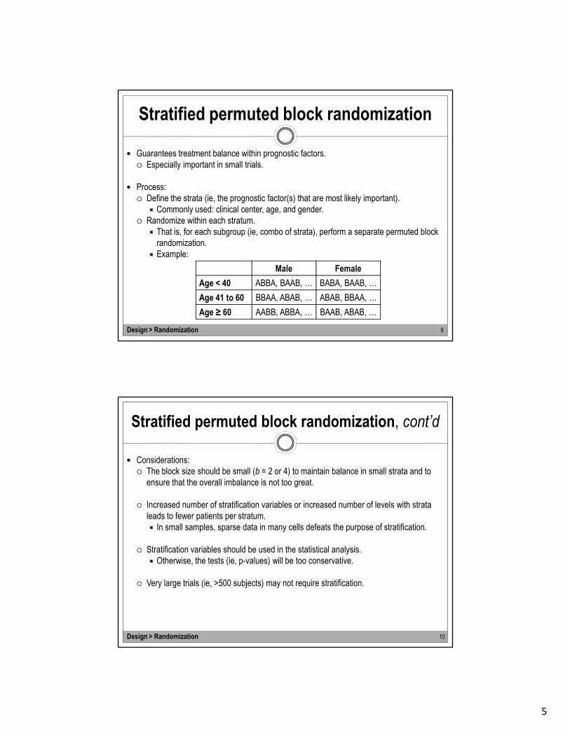
Stratified permuted block randomization

� Guarantees treatment balance within prognostic factors.

� Especially important in small trials.

� Process:

� Define the strata (ie, the prognostic factor(s) that are most likely important).

� Commonly used: clinical center, age, and gender.

� Randomize within each stratum.

� That is, for each subgroup (ie, combo of strata), perform a separate permuted block

randomization.

� Example:


Male Female

Age < 40 ABBA, BAAB, … BABA, BAAB, …

Age 41 to 60 BBAA, ABAB, … ABAB, BBAA, …

Age ≥ 60 AABB, ABBA, … BAAB, ABAB, …

10

Stratified permuted block randomization, cont’d

� Considerations:

� The block size should be small (b = 2 or 4) to maintain balance in small strata and to

ensure that the overall imbalance is not too great.

� Increased number of stratification variables or increased number of levels with strata

leads to fewer patients per stratum.

� In small samples, sparse data in many cells defeats the purpose of stratification.

� Stratification variables should be used in the statistical analysis.

� Otherwise, the tests (ie, p-values) will be too conservative.

� Very large trials (ie, >500 subjects) may not require stratification.


6

11

Implementation of randomization

� A set of standard operating procedures (SOPs) for the generation, implementation, and

administration of the randomization is required to ensure the integrity of a clinical trial.

� Clinician(s) and biostatistician(s) need to discuss the selection of the randomization

method and necessary information needed to generate the ‘randomization list’.

� The randomization method employed for the study should be described in detail in the

study protocol without disclosure of the block size, if permuted block randomization is

used.

� A formal request for the ‘randomization list’ cannot be sent unless the study protocol has

been obtained and approved by all necessary IRBs.


12

- Blinding -

Design

7

13

Blinding

� Keeping the identity of treatment assignments masked for:

� Subject

� Investigator (treatment team / evaluator)

� Monitoring committee (sponsor)

� Three possible types:

� Single-blind: subject does not know his/her treatment assignment.

� Double-blind: subject and investigator (treatment team / evaluator) do not know

treatment assignments.

� Triple-blind: subject, investigator (treatment team / evaluator), nor monitoring committee

(sponsor) do not know treatment assignments.

� Purpose: bias reduction.

� Each group blinded eliminates a different source of bias.

Design > Blinding

14

Reasons for blinding

� Reasons for subject blinding: if the treatment is known to the subject:

� Those on ‘no treatment’ or standard treatment may be discouraged and drop out of the

study.

� Those on the new drug may exhibit a placebo effect (ie, the new drug may appear

better when it actually is not).

� Subject reporting and cooperation may be biased depending on how the subject feels

about the treatment.

� Reasons for treatment team blinding: treatment can be biased by knowledge of the

treatment, especially if the treatment team has preconceived ideas about either treatment

through:

� Dose modifications,

� Intensity of patient examinations,

� Need for additional treatments,

� Influence on patient attitude through enthusiasm (or not) shown regarding the treatment.

Design > Blinding

8

15

Reasons for blinding, cont’d

� Reasons for evaluator blinding:

� If the endpoint is subjective, evaluator bias will lead to recording more favorable

responses on the preferred treatment.

� Even supposedly ‘hard’ endpoints (eg, blood pressure, MI) often require clinical

judgment.

� Reasons for monitoring committee blinding:

� Treatments can be objectively evaluated.

� Recommendations to stop the trial for ‘ethical’ reasons will not be based on personal

biases.

� NOTE: Triple-blind studies are hard to justify for reasons of safety and ethics.

→ Although blinded trials require extra effort, sometimes they are the only way to get an

objective answer to a clinical question.

Design > Blinding

16

Feasibility of blinding

� Ethics:

� The double-blind procedure should not result in any harm or undue risk to a patient.

� eg, may be unethical to give ‘simulated’ treatments to a control group.

� Practicality:

� May be impossible to blind some treatments (eg, radiation therapy equipment is usually

in constant use).

� Requiring a ‘sham’ treatment might be a poor use of resources.

� Avoidance of bias:

� Blinded studies require extra effort (eg, manufacturing look-alike pills, setting up coding

systems, etc).

� Consider the sources of bias to decide if the bias reduction is worth the extra effort.

� Compromise:

� Sometimes partial blinding (eg, independent blinded evaluators) can be sufficient to

reduce bias in treatment comparison.

Design > Blinding

9

17

- Sample size calculation -

Design

18

Preparing to calculate sample size

� 1. What is the main purpose of the trial?

� The question on which sample size is based.

� Most likely interested in assessing treatment differences.

� 2. What is the principal measure of patient outcome (ie, endpoint)?

� Continuous? Categorical? Time-to-event? Are some time-to-event values censored?

� 3. What statistical test will be used to assess treatment differences?

� Eg, t-test, chi-square, log-rank?

� What α-level are you assuming? Is your alternative hypothesis one-tailed or two-tailed?

� 4. What result is anticipated with the standard treatment?

� 5. How small a treatment difference is it important to detect and with what degree of

certainty (ie, power)?

Design > Sample size calculation

10

19

Example scenarios…

� Desire for both is to compare drug A (standard) to drug B (new).

� Dichotomous outcome:

� Want to test H0: pstandard = pnew vs Ha: pstandard ≠ pnew, where pstandard = proportion of

failures expected on drug A and pnew = proportion of failures on drug B.

� If an ‘event’ is a failure, want a reduced proportion on the new drug.

� Use PS > ‘Dichotomous’ tab.

� Continuous outcome:

� Want to test H0: meanstandard – meannew = 0 vs Ha: meanstandard – meannew ≠ 0.

� Eg, a 10 mg/dl difference (reduction) in cholesterol on the new drug.

� Additionally need an estimate of SD.

� Assume all observations are known completely (ie, no censoring).

� Assume data to be approximately normally distributed.

� Use PS > ‘t-test’ tab.


20

Example scenarios…, cont’d

� Time-to-event outcome:

� Want to test H0: median survival time on standard drug = median survival time on new

drug vs Ha: median survival time on standard drug ≠ median survival time on new drug.

� If an ‘event’ is a failure, want those on new drug to survive longer (ie, have large

median survival time).

� Similarly, want to test H0: hazard ratio of standard drug to new drug = 1 vs Ha: hazard

ratio of standard drug to new drug ≠ 1.

� If an ‘event’ is a failure, want those on new drug to have a smaller hazard of having

the event → hazard ratio of new drug to standard drug > 1.

� Additionally need estimates of

� (1) accrual time during which patients are recruited; and

� (2) additional follow-up time after the end of recruitment.

� General rule: accrual throughout the study period requires more patients that if all start

at the beginning of the study.

� Use PS > ‘Survival’ tab.


11

21

Additional consideration

� Adjustment for noncompliance (crossovers):

� If assume a new treatment is being compared with a standard treatment,

� Dropouts: those who refuse the new treatment some time after randomization and

revert to the standard treatment.

� Drop-ins: those who received the new treatment some time after initial randomization

to the standard treatment.

� Both generally dilute the treatment effect.

� Example: (dichotomous outcome)

� Suppose the true values are pdrug = 0.6 and pplacebo = 0.4 → ∆ = 0.6 – 0.4 = 0.2.

� Enroll N = 100 in each treatment group.

� Suppose 25% in drug group drop out and 10% in placebo group drop in.

� So, we actually observe pdrug = (75/100)*0.6 + (25/100)*0.4 = 0.55 and

pplacebo = (90/100)*0.4 + (10/100)*0.6 = 0.42 → ∆ = 0.55 – 0.42 = 0.13.

� The power of the study will be less than intended, or else the sample size must be

increased to compensate for the dilution effect.


22

- Baseline Assessment -

Analysis

12

23

Baseline Assessment

� Baseline data: collected before the start of the treatment (before or after randomization).

� Used to describe the population studied (ie, ‘Table 1’).

� Used to stratify, or at least check for balance over prognostic factors, demographic and

socioeconomic characteristics, and medical history data.

� NOTE: While randomization on average produces balance between groups, it does

not guarantee balance in any specific trial.

� Checking for treatment balance:

� Compare the baseline data for the subjects randomized to each treatment arm.

� Differences can be tested, but one should not conclude ‘no imbalance’ if p-values are

not significant (ie, > 0.5).

� Small sample sizes can lead to not rejecting H0 because of low power, even when

imbalance is present.

� Unless sample sizes are very large, rejecting H0 implies an imbalance problem that

should be addressed in the analysis.

Analysis > Baseline Assessment

24

- Intent-to-treat Analysis -

Analysis

13

25

Intent-to-treat analysis

� Under the intent-to-treat (ITT) principle, all randomized subjects should be included in the

(primary) analysis, in their assigned treatment groups, regardless of compliance (ie,

dropout or drop-in) with the assigned treatment.

� Rationale:

� Randomization ensures there are no systematic differences between treatment groups.

� The exclusion of patients from the analysis on a systematic basis (eg, lack of

compliance with assigned treatment) may introduce systematic difference between

treatment groups, thereby biasing the comparison.

� Arguments made against ITT analysis:

� In assessing the effect of a drug, it makes not sense to include in the treatment arm

subject who didn’t get the drug, or got too little drug to have any effect.

� The question of primary interest is whether the drugs works if used as intended.

� Food for thought: if in a randomized study an analysis is done which does not classify all

patients to the groups to which they were randomized, the study can no longer be strictly

interpreted as a randomized trial (ie, the randomization is ‘broken’).

Analysis > Baseline Assessment

26

- Kaplan-Meier Estimator and

Comparison of survival Curves -

Analysis

14

27

Survival analysis

� Set of methods for analyzing data where the outcome is the time until the occurrence of an

event of interest.

� A.k.a. ‘time-to-event’ analysis.

� Event often called ‘failure’ → a.k.a. analysis of failure time data.

� ‘Time-to-event’ outcome is common type of outcome in randomized clinical trials.

� Examples: time to cardiovascular death; time to tumor recurrence; time to a response

(10% decrease in BP).

� Distinguished by its emphasis on estimating the time course of events.

� Three requirements to determine failure time precisely:

� A time origin must be unambiguously defined.

� A scale for measuring the passage of time must be agreed upon.

� The meaning of failure (ie, the definition of the event) must be entirely clear.

� Each subject’s outcome has two components:

� (1) whether the subject experienced the event (No/Yes).

� (2) length of time between the time origin and the occurrence of the event or censoring.

Analysis > Kaplan-Meier Estimator and Comparison of Survival Curves

28

Censoring

� General idea: when the value of an observation is only partially known.

� Subjects not followed long enough for the event to have occurred have their ‘event

times’ censored at the time of last known follow-up.

� Types of censoring.

� Right: the time to the event is known to be greater than some value.

� Left: the time to the event is known to be less than some value.

� Interval: the time to the event is known to be in a specified interval.

� Type I: stop the RCT after a predetermined time (eg, at 2 years follow-up).

� Type II: stop the RCT after a predetermined number of events have occurred.

� Most statistical analyses assume that what causes a subject to be censored is

independent of what would cause him/her to have an event.

� If this is not the case, informative censoring is said to be present.

� Example: if a subject is pulled off of a drug because of a treatment failure, the censoring

time is indirectly reflecting a bad clinical outcome (resulting analysis will be biased).


15

29

Censoring, cont’d

� In addition to termination of the study, also result from:

� Loss to follow-up.

� Drop-out, which includes (for example) a patient who dies in an automobile accident

before relapsing.

� Illustration of censoring:


30

Kaplan-Meier (K-M) Estimator

� Procedure for estimating a survival curve (ie, the survival function) and its standard error.

� Survival function: probability of being free of the event at a specified time.

� Also can be thought as probability that a subject will ‘survive’ past a specified time.

� Non-increasing, step-wise (ie, not smooth) – a ‘step’ down for every event.

� Illustration of calculation:

� First, order to follow-up times,

either to event or censoring.

� Second, denote by indicator

variables whether the event

(or censoring occurred) at each

follow-up time.


16

Kaplan-Meier Estimator, cont’d

31

� Calculated K-M estimates most often

plotted, including the 95% CI.

� Hash marks (if shown) represent

censoring.

� From the K-M estimates, can determine:

� Median survival time (ie, time at which

Prob(Survival) = 50%).

� Probability of survival at a given time

point (ie, 1-year survival rate).

� K-M estimates can also be calculated

across a stratifying variable (eg, gender).

� Estimate the survival function in each

group of the stratifying variable (eg, a

set of estimates for females and a set of

estimates for males).


0 200 400 600 800 1000 1200

0.0

0.2

0.4

0.6

0.8

1.0

Time (days)

Pro

b(S

urv

ival)

32

Comparison of survival curves

� (Non-parametric) Log-rank test: a statistical method for comparing two or more survival

curves (ie, between (independent) groups).

� H0: the survival curves are equal vs Ha: the survival curves are not equal.

� More formally, H0: the probability of having an event in any group is equal (for all time

points during the study).

� Rejection of H0 indicates that the event rates differ between groups at one or more

time points during the study (ie, the probability of survival is different).

� Falls short in the following situations:

� When the survival curves cross at one or more points in time.

� Stratifying variable is a continuous variable (eg, age).

� Have more than one stratifying variable.

� When you want to quantify the difference between the survival curves.


17

Comparison of survival curves, cont’d

33

� For plot on right, log-rank p-value = 0.303.

� Conclusion: Failed to find a significant

difference between the two survival

curves.

� Plots can also include 95% Cis for each

curve – can be too busy.

� Plots can also include the number of

subjects at risk at specific time points –

often placed in lower margin.


0 200 400 600 800 1000 1200

0.0

0.2

0.4

0.6

0.8

1.0

Time (days)

Pro

b(S

urv

ival)

Drug A

Drug B

34

- Cox Proportional Hazards Model -

Analysis

18

35

Cox Proportional Hazards Model

� Widely used in the analysis of survival data to explain (ie, estimate) the effect of

explanatory variables on survival times.

� Proportional Hazards (PH) Models in general:

� Way of modeling the hazard function: the probability that the event of interest occurs at

a specified time t given that it has not occurred prior to time t.

� Can be thought of as the instantaneous rate at which events occur.

� Back to the Cox PH model…

� Widely used ‘semi-parametric’ approach that does not require the assumption of any

particular hazard function or distribution of survival time data.

� Proportional hazard assumption: requires that the ratio of hazards between any two

fixed sets of covariates not vary with time.

� That is, the event hazard rate may change over time, but the ratio of event hazards

between two groups of individuals is constant.

Analysis > Cox Proportional Hazards Model

36

Cox PH Model, cont’d

� Interpretation of model output:

� NOTE: assumes the effect of any predictors is the same for all values of time.

� The (raw estimated) regression coefficient for a covariate Xj is the increase/decrease

in the log hazard at any time point t if Xj is increased by one unit and all other

predictors are held constant.

� The effect of increasing Xj by 1 unit is to increase/decrease the hazard of the event by

a factor of exp(coefficient) at all points in time.

� exp(coefficient) also interpreted as a hazard ratio.

� Cox PH model output is most often reported in terms of estimated hazard ratios and

their 95% CIs.

� Do not report raw coefficients or p-values.

� If 95% CI contains the value 1, then estimated hazard ration is not significant.


19

37

Cox PH Model, cont’d

� Example:

� Estimating the effect of treatment, adjusted for age, on survival in a RCT comparing two

treatments (Treatment B and Treatment A) for ovarian cancer.

� Model output:

� Interpretation:

� The hazard of surviving for those who received Treatment B is 0.45 times that for

those who received Treatment A.

� The hazard of surviving is 1.16 times higher for each 1 year increase of age.

� The hazard of surviving is 2.17 times higher (exp(5*0.15)) for each 5 year

increase of age.

� We failed to find a significant effect of both treatment and age.


Coeff HR 95% CI of HR

Treatment B -0.80 0.45 (0.13, 1.55)

Age 0.15 1.16 (1.06, 1.27)

38

Do we really need survival analysis?

� Why not use linear regression to model the survival time as a function of a set of predictor

variables?

� Time to event is restricted to be positive, which has a skewed distribution.

� Change of interest – probability of surviving past a certain point in time.

� Cannot effectively handle the censoring of the observations.

� OK, so why not use logistic regression to model the dichotomous event outcome (ie, model

the probability of having an event)?

� As before, interested in the probability of surviving past a certain time point.

� As before, cannot effectively handle censoring.

� Will have lower power - only considering whether each subject had the event, not the

time until the subject possibly had the event.

� Also, inherently assuming that the time until the event is the same for all subjects.


20

39

- CONSORT Statement -

Reporting

40

CONSORT Statement

� Product of CONSORT – Consolidated Standards of Reporting Trials.

� http://www.consort-statement.org

� An evidence-based, minimum set of recommendations for reporting randomized clinical

trials.

� Offers a standard way for authors to prepare reports of trial findings, facilitating their

complete and transparent reporting, and aiding their critical appraisal and interpretation.

� Comprised of a 25-item checklist and a flow diagram.

� Checklist: focuses on reporting how the trial was designed, (conducted), analyzed, and

interpreted.

� Enables readers to assess the validity of the results.

� Flow diagram: displays the progress of all participants through the trial.

� Newest version - CONSORT 2010 Statement published on March, 2010.

Reporting > CONSORT Statement

21

41

The Checklist

� Title

� Identification as a randomized trial in the title.

� Abstract

� Structured summary of trial design, methods, results, and conclusions.

� Introduction

� Scientific background and explanation of rationale.

� Specific objectives or hypotheses.

� Methods

� Description of trial design (such as parallel, factorial) including allocation ratio.

� Eligibility criteria for participants.

� Settings and locations where the data were collected (ie, study settings).

� The interventions for each group with sufficient details to allow replication, including how

and when they were actually administered.

� Completely defined pre-specified primary and secondary outcome measures, including

how and when they were assessed.


42

The Checklist, cont’d

� Methods, cont’d

� Any changes to trial outcomes after the trial commenced, with reasons.

� How sample size was determined.

� When applicable, explanation of any interim analyses and stopping guidelines.

� Randomization

� Method used to generate the random allocation sequence.

� Type of randomization; details of any restriction (such as blocking and block size).

� Mechanism used to implement the random allocation sequence (such as

sequentially numbered containers), describing any steps taken to conceal the

sequence until interventions were assigned.

� Who generated the allocation sequence, who enrolled participants, and who

assigned participants to interventions.

� If done, who was blinded after assignment to interventions (for example, participants,

care providers, those assessing outcomes) and how.

� If relevant, description of the similarity of interventions.


22

43


� Methods, cont’d

� Statistical methods used to compare groups for primary and secondary outcomes.

� Methods for additional analyses, such as subgroup analyses and adjusted analyses.

� Results

� Participant flow diagram - for each group, the numbers of participants who were

randomly assigned, received intended treatment, and were analyzed for the primary

outcome (see accompanying handout).

� For each group, losses and exclusions after randomization, together with reasons.

� Dates defining the periods of recruitment and follow-up.

� Why the trial ended or was stopped (ie, reason(s) for stopped trial).

� A table showing baseline demographic and clinical characteristics for each group.

� For each group, number of participants (denominator) included in each analysis (ie,

numbers analyzed) and whether the analysis was an ‘intention-to-treat analysis’.

� For each primary and secondary outcome, results for each group, and the estimated

effect size and its precision (such as 95% confidence interval).


44


� Results, cont’d

� Results of any other analyses performed, including subgroup analyses and adjusted

analyses, distinguishing pre-specified from exploratory.

� All important harms or unintended effects in each group (ie, harms/adverse events).

� Discussion

� Trial limitations, addressing sources of potential bias, imprecision, and, if relevant,

multiplicity of analyses.

� Generalizability (external validity, applicability) of the trial findings.

� Interpretation consistent with results, balancing benefits and harms, and considering

other relevant evidence.

� Other Information

� Registration number and name of trial registry (clinicaltrials.gov).

� Where the full trial protocol can be accessed, if available.

� Sources of funding and other support (such as supply of drugs), role of funders.


23

45

• ‘Designing Clinical Research’ by Hulley et al (3rd edition).

• Vanderbilt’s ‘Clinical Trials’ MPH course.

• Class notes provided by Yu Shyr, PhD.

• Additional lecture notes provided by Fei Ye, PhD and Zhigou (Alex) Zhao,

MS.

References

clinical trials: statistical...

Documents