5/1 ETH Zurich – Distributed Computing – www.disco.ethz.ch

Roger Wattenhofer

Clock Synchronization Part 2, Chapter 5

TexPoint fonts used in EMF. Read the TexPoint manual before you delete this box.: AAAAA

5/2

Clock Synchronization

5/3

• Motivation

• Real World Clock Sources, Hardware and Applications

• Clock Synchronization in Distributed Systems

• Theory of Clock Synchronization

• Protocol: PulseSync

Overview

5/4

Motivation

• Logical Time (“happened-before”)

• Determine the order of events in a distributed system

• Synchronize resources

• Physical Time

• Timestamp events (email, sensor data, file access times etc.)

• Synchronize audio and video streams

• Measure signal propagation delays (Localization)

• Wireless (TDMA, duty cycling)

• Digital control systems (ESP, airplane autopilot etc.)

5/5

Properties of Clock Synchronization Algorithms

• External vs. internal synchronization

– External sync: Nodes synchronize with an external clock source (UTC)

– Internal sync: Nodes synchronize to a common time

– to a leader, to an averaged time, ...

• One-shot vs. continuous synchronization

– Periodic synchronization required to compensate clock drift

• Online vs. offline time information

– Offline: Can reconstruct time of an event when needed

• Global vs. local synchronization (explained later)

• Accuracy vs. convergence time, Byzantine nodes, …

5/6

World Time (UTC)

• Atomic Clock

– UTC: Coordinated Universal Time

– SI definition 1s := 9192631770 oscillation cycles of the caesium-133 atom

– Clocks excite these atoms to oscillate and count the cycles

– Almost no drift (about 1s in 10 Million years)

– Getting smaller and more energy efficient!

5/7

Atomic Clocks vs. Length of a Day

5/8

Access to UTC

• Radio Clock Signal

– Clock signal from a reference source (atomic clock) is transmitted over a long wave radio signal

– DCF77 station near Frankfurt, Germany transmits at 77.5 kHz with a transmission range of up to 2000 km

– Accuracy limited by the propagation delay of the signal, Frankfurt-Zurich is about 1ms

– Special antenna/receiver hardware required

5/9

What is UTC, really?

• International Atomic Time (TAI)

– About 200 atomic clocks

– About 50 national laboratories

– Reduce clock skew by comparing and averaging

– UTC = TAI + UTC leap seconds (irregular rotation of earth)

• GPS

– USNO Time

– USNO vs. TAI difference is a few nanoseconds

5/10

Comparing (and Averaging)

Station A Station B

𝑡Δ𝐴 = 𝑡𝐴 − (𝑡𝑆𝑉+𝑑𝐴) 𝑡Δ𝐵 = 𝑡𝐵 − (𝑡𝑆𝑉+𝑑𝐵)

𝑑𝐵 𝑑𝐴

𝑡Δ = 𝑡Δ𝐵 − 𝑡Δ𝐴 = 𝑡𝐵 − 𝑡𝑆𝑉 + 𝑑𝐵 − 𝑡𝐴 + 𝑡𝑆𝑉 + 𝑑𝐴 = 𝑡𝐵 − 𝑡𝐴 + 𝑑𝐴 − 𝑑𝐵

5/11

Global Positioning System (GPS)

• Satellites continuously transmit own position and time code

• Line of sight between satellite and receiver required

• Special antenna/receiver hardware required

• Time of flight of GPS signals varies between 64 and 89ms

• Positioning in space and time!

• What is more accurate, GPS or Radio Clock Signal?

5/12

GPS Localization

Assuming that time of GPS satellites is correctly synchronized…

𝑡2 𝑡𝑆𝑉 𝑡1 𝑡4 𝑡3 𝑟1 𝑟2 𝑟3 𝑟4

𝑡12 𝑡13

𝑡14

𝑡𝑅

𝑡

𝑡 − 𝑡1

𝑡 + 𝑡12 − 𝑡2

𝑡 + 𝑡13 − 𝑡3 𝑡 + 𝑡14 − t4

𝒔𝟏

𝒔𝟒 𝒔𝟑

𝒔𝟐

𝒑

5/13

𝒔𝟏 − 𝒑

𝑐= 𝑡 − 𝑡1

𝒔𝟐 − 𝒑

𝑐= 𝑡 + 𝑡12 − 𝑡2

𝒔𝟑 − 𝒑

𝑐= 𝑡 + 𝑡13 − 𝑡3

⋮ ⋮

𝒔𝒏 − 𝒑

𝑐= 𝑡 + 𝑡1𝑛 − 𝑡𝑛

𝑐 = speed of light

Find least squares solution in 𝑡 and 𝒑

𝒔𝟒

GPS Localization

𝑡 − 𝑡1

𝑡 + 𝑡12 − 𝑡2

𝑡 + 𝑡13 − 𝑡3 𝑡 + 𝑡14 − t4

𝒔𝟏

𝒔𝟑

𝒔𝟐

𝒑

5/14

Keeping GPS Satellites synchronized

5/15

Alternative (Silly) Clock Sources

• AC power lines

– Use the magnetic field radiating from electric AC power lines

– AC power line oscillations are extremely stable (drift about 10 ppm, ppm = parts per million)

– Power efficient, consumes only 58 μW

– Single communication round required to correct phase offset after initialization

• Sunlight

– Using a light sensor to measure the length of a day

– Offline algorithm for reconstructing global timestamps by correlating annual solar patterns (no communication required)

5/16

Clock Devices in Computers

• Real Time Clock (IBM PC)

• Battery backed up

• 32.768 kHz oscillator + Counter

• Get value via interrupt system

• HPET (High Precision Event Timer)

• Oscillator: 10 Mhz … 100 Mhz

• Up to 10 ns resolution!

• Schedule threads

• Smooth media playback

• Usually inside Southbridge

5/17

Clock Drift

• Clock drift: random deviation from the nominal rate dependent on power supply, temperature, etc.

• E.g. TinyNodes have a maximum drift of 30-50 ppm (parts per million)

This is a drift of up to 50μs per second or 0.18s per hour

t

rate

1 1+²

1-²

5/18

Clock Synchronization in Computer Networks

• Network Time Protocol (NTP)

• Clock sync via Internet/Network (UDP)

• Publicly available NTP Servers (UTC)

• You can also run your own server!

• Packet delay is estimated to reduce clock skew

5/19

Propagation Delay Estimation (NTP)

• Measuring the Round-Trip Time (RTT)

• Propagation delay 𝛿 and clock skew Θ can be calculated

B

A Time accor- ding to A

Request from A

Answer from B

Time accor- ding to B

𝛿 =𝑡4 − 𝑡1 − (𝑡3 − 𝑡2)

2

Θ =𝑡2 − (𝑡1 + 𝛿) − (𝑡4 − (𝑡3 + 𝛿))

2=

𝑡2 − 𝑡1 + (𝑡3 − 𝑡4)

2

𝑡2

𝑡1 𝑡4

𝑡3

5/20

Reception Callback

Problem: Jitter in the message delay

Various sources of errors (deterministic and non-deterministic)

Solution: Timestamping packets at the MAC layer

→ Jitter in the message delay is reduced to a few clock ticks

Messages Experience Jitter in the Delay

0-100 ms 0-500 ms 1-10 ms

0-100 ms

t

SendCmd Access Transmission

5/21

Jitter Measurements

• Different radio chips use different paradigms

– Left is a CC1000 radio chip which generates an interrupt with each byte.

– Right is a CC2420 radio chip that generates a single interrupt for the packet after the start frame delimiter is received.

• In wireless networks propagation can be ignored (<1¹s for 300m).

• Still there is quite some variance in transmission delay because of latencies in interrupt handling (picture right).

5/22

• Precision Time Protocol (PTP) is very similar to NTP

• Commodity network adapters/routers/switches can assist in time sync by timestamping PTP packets at the MAC layer

• Packet delay is only estimated on request

• Synchronization through one packet from server to clients!

• Some newer hardware (1G Intel cards, 82580) can timestamp any packet at the MAC layer

• Achieving skew of about 1 microsecond

Clock Synchronization in Computer Networks (PTP)

5/23

• Synchronous digital circuits require all components to act in sync

• The bigger the clock skew, the longer the clock period

• The clock signal that governs this rhythm needs to be distributed to all components such that skew and wire length is minimized

• Optimize routing, insert buffers (also to improve signal)

Hardware Clock Distribution

10 15

20

15

9

20 20

20

20

20

12 20

5/24

• Reference Broadcast Synchronization (RBS) Synchronizing atomic clocks

• Sender synchronizes set of clocks

• Time-sync Protocol for Sensor Networks (TPSN) Network Time Protocol

• Estimating round trip time to sync more accurately

• Flooding Time Synchronization Protocol (FTSP)Precision Time Protocol

• Timestamp packets at the MAC Layer to improve accuracy

Clock Synchronization Tricks in Wireless Networks

1

A

0

1

2 2

B

2

𝑡3

𝑡4 𝑡1

𝑡2

A

B S

Θ

𝑡2

t1

4

6

1

2 3

5

7

0

5/25

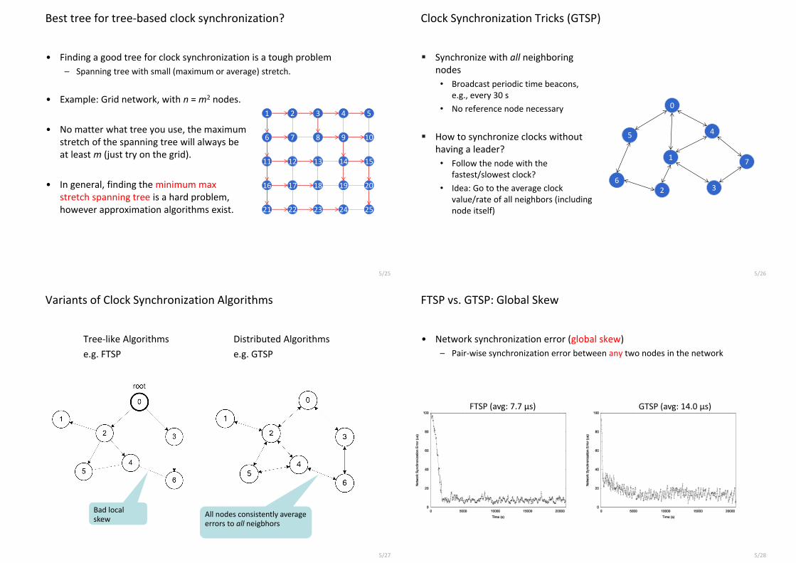
Best tree for tree-based clock synchronization?

• Finding a good tree for clock synchronization is a tough problem

– Spanning tree with small (maximum or average) stretch.

• Example: Grid network, with n = m2 nodes.

• No matter what tree you use, the maximum stretch of the spanning tree will always be at least m (just try on the grid).

• In general, finding the minimum max stretch spanning tree is a hard problem, however approximation algorithms exist.

1 2 3 4 5

6 7 8 9 10

11 12 13 14 15

16 17 18 19 20

21 22 23 24 25

5/26

Synchronize with all neighboring nodes

• Broadcast periodic time beacons, e.g., every 30 s

• No reference node necessary

How to synchronize clocks without having a leader?

• Follow the node with the fastest/slowest clock?

• Idea: Go to the average clock value/rate of all neighbors (including node itself)

Clock Synchronization Tricks (GTSP)

4

6

1

2 3

5

7

0

5/27

Variants of Clock Synchronization Algorithms

Tree-like Algorithms Distributed Algorithms

e.g. FTSP e.g. GTSP

Bad local skew

All nodes consistently average errors to all neigbhors

5/28

FTSP vs. GTSP: Global Skew

• Network synchronization error (global skew)

– Pair-wise synchronization error between any two nodes in the network

FTSP (avg: 7.7 μs) GTSP (avg: 14.0 μs)

5/29

FTSP vs. GTSP: Local Skew

• Neighbor Synchronization error (local skew)

– Pair-wise synchronization error between neighboring nodes

• Synchronization error between two direct neighbors:

FTSP (avg: 15.0 μs) GTSP (avg: 2.8 μs)

5/30

Global vs. Local Time Synchronization

• Common time is essential for many applications:

– Assigning a timestamp to a globally sensed event (e.g. earthquake)

– Precise event localization (e.g. shooter detection, multiplayer games)

– TDMA-based MAC layer in wireless networks

– Coordination of wake-up and sleeping times (energy efficiency)

5/31

• Given a communication network

1. Each node equipped with hardware clock with drift

2. Message delays with jitter

• Goal: Synchronize Clocks (“Logical Clocks”)

• Both global and local synchronization!

Theory of Clock Synchronization

worst-case (but constant)

5/32

• Time (logical clocks) should not be allowed to stand still or jump

• Let’s be more careful (and ambitious):

• Logical clocks should always move forward

• Sometimes faster, sometimes slower is OK.

• But there should be a minimum and a maximum speed.

• As close to correct time as possible!

Time Must Behave!

5/33

Formal Model

• Hardware clock Hv(t) = s[0,t] hv(¿) d¿ with clock rate hv(t) 2 [1-²,1+²]

• Logical clock Lv(∙) which increases at rate at least 1 and at most ¯

• Message delays 2 [0,1]

• Employ a synchronization algorithm to update the logical clock according to hardware clock and messages from neighbors

Clock drift ² is typically small, e.g. ² ¼10-4 for a cheap quartz oscillator

Neglect fixed share of delay, normalize jitter

Logical clocks with rate less than 1 behave differently (“synchronizer”)

Time is 140 Time is 150

Time is 152

Lv?

Hv

5/34

Synchronization Algorithms: An Example (“Amax”)

• Question: How to update the logical clock based on the messages from the neighbors?

• Idea: Minimizing the skew to the fastest neighbor

– Set the clock to the maximum clock value received from any neighbor (if larger than local clock value)

– forward new values immediately

• Optimum global skew of about D

• Poor local property

– First all messages take 1 time unit…

– …then we have a fast message!

Time is D+x Time is D+x

…

Clock value: D+x

Old clock value: D+x-1

Old clock value: x+1

Old clock value: x

Time is D+x

New time is D+x New time is D+x skew D!

Allow ¯ = 1

Fastest Hardware

Clock

5/35

Synchronization Algorithms: Amax’

• The problem of Amax is that the clock is always increased to the maximum value

• Idea: Allow a constant slack γ between the maximum neighbor clock value and the own clock value

• The algorithm Amax’ sets the local clock value Li(t) to 𝐿𝑖 𝑡 ≔ max(𝐿𝑖 𝑡 ,max𝑗∈𝑁𝑖

𝐿𝑗 𝑡 − 𝛾)

→ Worst-case clock skew between two neighboring nodes is still Θ(D) independent of the choice of γ!

• How can we do better?

– Adjust logical clock speeds to catch up with fastest node (i.e. no jump)?

– Idea: Take the clock of all neighbors into account by choosing the average value?

L i (t) := max (L i (t))test i (t)

5/36

Local Skew: Overview of Results

1 logD √D D …

Everybody‘s expectation, five years ago („solved“)

Lower bound of logD / loglogD [Fan & Lynch, PODC 2004]

All natural algorithms [Locher et al., DISC 2006]

Blocking algorithm

Kappa algorithm [Lenzen et al., FOCS 2008]

Tight lower bound [Lenzen et al., PODC 2009]

Dynamic Networks! [Kuhn et al., SPAA 2009]

5/37

Enforcing Clock Skew

• Messages between two neighboring nodes may be fast in one direction and slow in the other, or vice versa.

• A constant skew between neighbors may be „hidden“.

• In a path, the global skew may be in the order of D/2.

2 3 4 5 6 7

2 3 4 5 6 7

2 3 4 5 6 7

2 3 4 5 6 7

2 3 4 5 6 7

2 3 4 5 6 7

u

v

5/38

Local Skew: Lower Bound

Theorem: (logβ−1𝜖 D) skew between neighbors

• Add 𝑙0 2 skew in 𝑙0 2𝜖 time, messing with clock rates and messages

• Afterwards: Continue execution for 𝑙0 4(𝛽−1) time (all ℎ𝑥 = 1)

Skew reduces by at most 𝑙0 4 at least 𝑙0 4 skew remains

Consider a subpath of length 𝑙1 = 𝑙0 ⋅𝜖2 𝛽−1 with at least 𝑙1 4 skew

Add 𝑙1 2 skew in 𝑙1 2𝜖 = 𝑙04(𝛽−1) time at least 3 4 ⋅ 𝑙1skew in subpath

• Repeat this trick (+½,-¼,+½,-¼,…) log2(β−1)𝜖 D times

Higher clock rates

𝑙0 = 𝐷

ℎ𝑣 = 1

ℎ𝑤 = 1 𝐿𝑤(𝑡)

𝐿𝑣(𝑡)=x

ℎ𝑤 = 1 𝐿𝑤(𝑡)

𝐿𝑣 𝑡 = 𝑥 +𝑙0

2 ℎ𝑣 = 1 + 𝜖

5/39

Local Skew: Upper Bound

• Surprisingly, up to small constants, the (log(¯-1)/² D) lower bound can be matched with clock rates 2 [1,¯] (tough part, not included)

• We get the following picture [Lenzen et al., PODC 2009]:

• In practice, we usually have 1/² ¼ 104 > D. In other words, our initial intuition of a constant local skew was not entirely wrong!

max rate ¯ 1+² 1+£(²) 1+√² 2 large

local skew 1 £(log D) £(log1/² D) £(log1/² D) £(log1/² D)

... because too large clock rates will amplify

the clock drift ².

We can have both smooth and accurate

clocks!

5/40

Sending periodic beacon messages to synchronize nodes

Back to Practice: Synchronizing Nodes

J

t=100 t=130

Beacon interval B

1

0

J

reference clock t

t

100 130

jitter jitter

5/41

Message delay jitter affects clock synchronization quality

How accurately can we synchronize two nodes?

y(x) = r∙x + ∆y

clock offset

^

relative clock rate (estimated)

0

1 x

y

J J ∆y

Beacon interval B

r ̂

r r ̂

5/42

Lower Bound on the clock skew between two neighbors

Clock Skew between two Nodes

Error in the rate estimation: Jitter in the message delay Beacon interval Number of beacons k

Synchronization error:

0

1 x

y

J J ∆y

Beacon interval B

r ̂

r r ̂

5/43

Nodes forward their current estimate of the reference clock

Each synchronization beacon is affected by a random jitter J

Sum of the jitter grows with the square-root of the distance

stddev(J1 + J2 + J3 + J4 + J5 + ... Jd) = √d×stddev(J)

Multi-hop Clock Synchronization

J1 J2 J3

0 1 2 3 4 ...

J4 J5

d

Single-hop: Multi-hop:

Jd

5/44

FTSP uses linear regression to compensate for clock drift

Jitter is amplified before it is sent to the next hop

Linear Regression (e.g. FTSP)

0

1 x

y

r

J J

∆y

Beacon interval B

Example for k=2

^

r

synchronization error

y(x) = r∙x + ∆y

clock offset

^

relative clock rate (estimated)

5/45

The PulseSync Protocol

• Send fast synchronization pulses through the network

Speed-up the initialization phase

Faster adaptation to changes in temperature or network topology

Beacon time B

t

0

1

2

3

4

t

0

1

2

3

4

FTSP

PulseSync

Expected time = D·B/2

Expected time = D·tpulse

tpulse

Beacon time B

5/46

The PulseSync Protocol (2)

• Remove self-amplification of synchronization error

Fast flooding cannot completely eliminate amplification

synchronization error

^

The green line is calculated using k measurement points that are

statistically independent of the red line.

0

1 x

y

r

J J

∆y

Beacon interval B

Example for k=2

^

r

y(x) = r∙x + ∆y

clock offset

relative clock rate (estimated)

5/47

FTSP vs. PulseSync

• Global Clock Skew

• Maximum synchronization error between any two nodes

Synchronization Error FTSP PulseSync

Average (t>2000s) 23.96 µs 4.44 µs

Maximum (t>2000s) 249 µs 38 µs

FTSP PulseSync

5/48

FTSP vs. PulseSync

• Sychnronization Error vs. distance from root node

FTSP PulseSync

5/49

Credits

• Approximation algorithms for minimum max stretch spanning tree, e.g. Emek and Peleg, 2004.

• More credits to come

5/50 ETH Zurich – Distributed Computing – www.disco.ethz.ch

Roger Wattenhofer

That’s all! Questions & Comments?

TexPoint fonts used in EMF. Read the TexPoint manual before you delete this box.: AAAAAAA