304

CHAPTER 12Closure in Valuation:

Estimating Terminal Value

In the previous chapter, we examined the determinants of expected growth. Firmsthat reinvest substantial portions of their earnings and earn high returns on these

investments should be able to grow at high rates. But for how long? This chapterbrings closure to firm valuation by considering this question.

As a firm grows, it becomes more difficult for it to maintain high growth and iteventually will grow at a rate less than or equal to the growth rate of the economyin which it operates. This growth rate, labeled stable growth, can be sustained inperpetuity, allowing us to estimate the value of all cash flows beyond that point as aterminal value for a going concern. The key question that we confront is the estima-tion of when and how this transition to stable growth will occur for the firm that weare valuing. Will the growth rate drop abruptly at a point in time to a stable growthrate or will it occur more gradually over time? To answer these questions, we willlook at a firm’s size (relative to the market that it serves), its current growth rate,and its competitive advantages.

We also consider an alternate route, which is that firms do not last forever andthat they will be liquidated at some point in the future. We will consider how best toestimate liquidation value and when it makes more sense to use this approachrather than the going concern approach.

CLOSURE IN VALUATION

Since you cannot estimate cash flows forever, you generally impose closure in dis-counted cash flow valuation by stopping your estimation of cash flows sometime inthe future and then computing a terminal value that reflects the value of the firm atthat point.

You can find the terminal value in one of three ways. One is to assume a liqui-dation of the firm’s assets in the terminal year and estimate what others would payfor the assets that the firm has accumulated at that point. The other two approachesvalue the firm as a going concern at the time of the terminal value estimation. Oneapplies a multiple to earnings, revenues, or book value to estimate the value in the

Value of a firmCF

k

Terminal value

( kt

ct

t 1

t nn

cn

=+

++=

=

∑( ) )1 1

ch12_p304-322.qxd 12/5/11 2:14 PM Page 304

terminal year. The other assumes that the cash flows of the firm will grow at a con-stant rate forever—a stable growth rate. With stable growth, the terminal value canbe estimated using a perpetual growth model.

Liquidation Value

In some valuations, we can assume that the firm will cease operations at a point intime in the future and sell the assets it has accumulated to the highest bidders. Theestimate that emerges is called a liquidation value. There are two ways in which theliquidation value can be estimated. One is to base it on the book value of the assets,adjusted for any inflation during the period. Thus, if the book value of assets 10years from now is expected to be $2 billion, the average age of the assets at thatpoint is five years and the expected inflation rate is 3 percent, the expected liquida-tion value can be estimated as:

Expected liquidation value = Book value of assetsterm year(1 + Inflation rate)average life of assets

= $2 billion(1.03)5 = $2.319 billion

The limitation of this approach is that it is based on accounting book value anddoes not reflect the earning power of the assets.

The alternative approach is to estimate the value based on the earning power ofthe assets. To make this estimate, we would first have to estimate the expected cashflows from the assets and then discount these cash flows back to the present, usingan appropriate discount rate. In the example above, for instance, if we assumedthat the assets in question could be expected to generate $400 million in after-taxcash flows for 15 years (after the terminal year) and the cost of capital was 10 per-cent, our estimate of the expected liquidation value would be:

When valuing equity, there is one additional step that needs to be taken. Theestimated value of debt outstanding in the terminal year has to be subtracted fromthe liquidation value to arrive at the liquidation proceeds for equity investors.

Multiple Approach

In this approach, the value of a firm in a future year is estimated by applying a multi-ple to the firm’s earnings or revenues in that year. For instance, a firm with expectedrevenues of $6 billion 10 years from now will have an estimated terminal value inthat year of $12 billion, if a value-to-sales multiple of 2 is used. If valuing equity, weuse equity multiples such as price-earnings ratios to arrive at the terminal value.

Although this approach has the virtue of simplicity, the multiple has a huge ef-fect on the final value and where it is obtained can be critical. If, as is common, themultiple is estimated by looking at how comparable firms in the business today arepriced by the market, the valuation becomes a relative valuation, rather than a dis-counted cash flow valuation. If the multiple is estimated using fundamentals, it con-verges on the stable growth model that will be described in the next section.

Expected liquidation value $400 million(PV of annuity, 15 years @ 10%) billion

== $ .3 042

Closure in Valuation 305

ch12_p304-322.qxd 12/5/11 2:14 PM Page 305

All in all, using multiples to estimate terminal value, when those multiplesare estimated from comparable firms, results in a dangerous mix of relative anddiscounted cash flow valuation. While there are advantages to relative valua-tion, and we consider these in a later chapter, a discounted cash flow valuationshould provide you with an estimate of intrinsic value, not relative value. Con-sequently, the only consistent way of estimating terminal value in a discountedcash flow model is to use either a liquidation value or to use a stable growthmodel.

Stable Growth Model

In the liquidation value approach, you are assuming that your firm has a finite lifeand that it will be liquidated at the end of that life. Firms, however, can reinvestsome of their cash flows back into new assets and extend their lives. If you assumethat cash flows, beyond the terminal year, will grow at a constant rate forever, theterminal value can be estimated as follows:

Terminal valuet = Cash flowt+1/(r − Stable growth)

The cash flow and the discount rate used will depend on whether you are valuingthe firm or valuing equity. If we are valuing equity, the terminal value of equity canbe written as:

Terminal value of equityn = Cash flow to equityn+1/(Cost of equityn+1 − gn)

The cash flow to equity can be defined strictly as dividends (in the dividend dis-count model) or as free cash flow to equity. If valuing a firm, the terminal value canbe written as:

Terminal valuen = Free cash flow to firmn+1/(Cost of capitaln+1 − gn)

where the cost of capital and the growth rate in the model are sustainableforever.

In this section, we will begin by considering how high a stable growth rate canbe, how to best estimate when your firm will be a stable growth firm, and what in-puts need to be adjusted as a firm approaches stable growth.

Constraints on Stable Growth Of all the inputs into a discounted cash flow valua-tion model, none can affect the value more than the stable growth rate. Part of thereason for it is that small changes in the stable growth rate can change the terminalvalue significantly, and the effect gets larger as the growth rate approaches the dis-count rate used in the estimation. Not surprisingly, analysts often use it to alter thevaluation to reflect their biases.

The fact that a stable growth rate is constant forever, however, puts strongconstraints on how high it can be. Since no firm can grow forever at a rate higherthan the growth rate of the economy in which it operates, the constant growth rate

306 CLOSURE IN VALUATION: ESTIMATING TERMINAL VALUE

ch12_p304-322.qxd 12/5/11 2:14 PM Page 306

cannot be greater than the overall growth rate of the economy. In making a judg-ment on what the limits on stable growth rate are, we have to consider the follow-ing three questions:

1. Is the company constrained to operate as a domestic company, or does it op-erate (or have the capacity to operate) multinationally? If a firm is a purely domes-tic company, either because of internal constraints (such as those imposed bymanagement) or external (such as those imposed by a government), the growth ratein the domestic economy will be the limiting value. If the company is a multina-tional or has aspirations to be one, the growth rate in the global economy (or atleast those parts of the globe that the firm operates in) will be the limiting value.

2. Is the valuation being done in nominal or real terms? If the valuation is anominal valuation, the stable growth rate should also be a nominal growth rate(i.e., include an expected inflation component). If the valuation is a real valua-tion, the stable growth rate will be constrained to be lower. Again, using Coca-Cola as an example, the stable growth rate can be as high as 5.5 percent if thevaluation is done in nominal U.S. dollars but only 3 percent if the valuation isdone in real dollars.

3. What currency is being used to estimate cash flows and discount rates inthe valuation? The limits on stable growth will vary depending on what currencyis used in the valuation. If a high-inflation currency is used to estimate cash flowsand discount rates, the stable growth rate will be much higher, since the expectedinflation rate is added on to real growth. If a low-inflation currency is used to estimate cash flows, the stable growth rate will be much lower. For instance, the stable growth rate that would be used to value Titan Cement, the Greek cement company, will be much higher if the valuation is done in drachmas thanin euros.

While the stable growth rate cannot exceed the growth rate of the economyin which a firm operates, it can be lower. There is nothing that prevents us from assuming that mature firms will become a smaller part of the economy andit may, in fact, be the more reasonable assumption to make. Note that thegrowth rate of an economy reflects the contributions of both young, higher-growth firms and mature, stable-growth firms. If the former grow at a rate muchhigher than the growth rate of the economy, the latter have to grow at a rate thatis lower.

Setting the stable growth rate to be less than or equal to the growth rate of theeconomy is not only the consistent thing to do but it also ensures that the growthrate will be less than the discount rate. This is because of the relationship betweenthe riskless rate that goes into the discount rate and the growth rate of the econ-omy. Note that the riskless rate can be written as:

Nominal riskless rate = Real riskless rate + Expected inflation rate

In the long term, the real riskless rate will converge on the real growth rate ofthe economy, and the nominal riskless rate will approach the nominal growth rateof the economy. In fact, a simple rule of thumb on the stable growth rate is that itgenerally should not exceed the riskless rate used in the valuation.

Closure in Valuation 307

ch12_p304-322.qxd 12/5/11 2:14 PM Page 307

Key Assumptions about Stable Growth In every discounted cash flow valuation,there are three critical assumptions you need to make on stable growth. The first re-lates to when the firm that you are valuing will become a stable growth firm, if it isnot one already. The second relates to what the characteristics of the firm will be instable growth, in terms of return on investments and costs of equity and capital.The final assumption relates to how the firm that you are valuing will make thetransition from high growth to stable growth.

Length of the High Growth Period The question of how long a firm will beable to sustain high growth is perhaps one of the more difficult questions to an-swer in a valuation, but two points are worth making. One is that it is not aquestion of whether but when firms hit the stable growth wall. All firms ulti-mately become stable growth firms, in the best case, because high growth makesa firm larger, and the firm’s size will eventually become a barrier to further highgrowth. In the worst-case scenario, firms may not survive and will be liquidated.The second is that high growth in valuation, or at least high growth that createsvalue,1 comes from firms earning excess returns on their marginal investments.In other words, increased value comes from firms having a return on capital thatis well in excess of the cost of capital (or a return on equity that exceeds the costof equity). Thus, when you assume that a firm will experience high growth forthe next 5 or 10 years, you are also implicitly assuming that it will earn excessreturns (over and above the required return) during that period. In a competitivemarket, these excess returns will eventually draw in new competitors, and theexcess returns will disappear.

308 CLOSURE IN VALUATION: ESTIMATING TERMINAL VALUE

CAN THE STABLE GROWTH RATE BE NEGATIVE?

The previous section noted that the stable growth rate has to be less than orequal to the growth rate of the economy. But can it be negative? There is noreason why not since the terminal value can still be estimated. For instance, afirm with $100 million in after-tax cash flows growing at –5% a year foreverand a cost of capital of 10 percent has a value of:

Value of firm = 100(1 − .05)/[.10 − (−.05)] = $633 million

Intuitively, though, what does a negative growth rate imply? It essentially al-lows a firm to partially liquidate itself each year until it just about disappears.Thus, it is an intermediate choice between complete liquidation and the goingconcern that gets larger each year forever.

This may be the right choice to make when valuing firms in industries thatare being phased out because of technological advances (such as the manufac-turers of typewriters, with the advent of the personal computer) or where anexternal and critical customer is scaling back purchases for the long term (aswas the case with defense contractors after the end of the cold war).

1Growth without excess returns will make a firm larger but not add value.

ch12_p304-322.qxd 12/5/11 2:14 PM Page 308

You should look at three factors when considering how long a firm will be ableto maintain high growth.

1. Size of the firm. Smaller firms are much more likely to earn excess returns andmaintain these excess returns than otherwise similar larger firms. This is be-cause they have more room to grow and a larger potential market. Small firmsin large markets should have the potential for high growth (at least in revenues)over long periods. When looking at the size of the firm, you should look notonly at its current market share, but also at the potential growth in the totalmarket for its products or services. A firm may have a large market share of itscurrent market, but it may be able to grow in spite of this because the entiremarket is growing rapidly.

2. Existing growth rate and excess returns. Momentum does matter, when itcomes to projecting growth. Firms that have been reporting rapidly growingrevenues are more likely to see revenues grow rapidly at least in the near future.Firms that are earning high returns on capital and high excess returns in thecurrent period are likely to sustain these excess returns for the next few years.

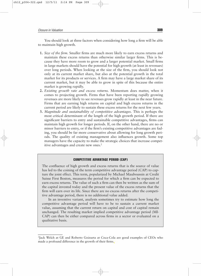
3. Magnitude and sustainability of competitive advantages. This is perhaps themost critical determinant of the length of the high growth period. If there aresignificant barriers to entry and sustainable competitive advantages, firms canmaintain high growth for longer periods. If, on the other hand, there are no orminor barriers to entry, or if the firm’s existing competitive advantages are fad-ing, you should be far more conservative about allowing for long growth peri-ods. The quality of existing management also influences growth. Some topmanagers have the capacity to make the strategic choices that increase compet-itive advantages and create new ones.2

Closure in Valuation 309

COMPETITIVE ADVANTAGE PERIOD (CAP)

The confluence of high growth and excess returns that is the source of valuehas led to the coining of the term competitive advantage period (CAP) to cap-ture the joint effect. This term, popularized by Michael Mauboussin at CreditSuisse First Boston, measures the period for which a firm can be expected toearn excess returns. The value of such a firm can then be written as the sum ofthe capital invested today and the present value of the excess returns that thefirm will earn over its life. Since there are no excess returns after the competi-tive advantage period, there is no additional value added.

In an inventive variant, analysts sometimes try to estimate how long thecompetitive advantage period will have to be to sustain a current marketvalue, assuming that the current return on capital and cost of capital remainunchanged. The resulting market implied competitive advantage period (MI-CAP) can then be either compared across firms in a sector or evaluated on aqualitative basis.

2Jack Welch at GE and Roberto Goizueta at Coca-Cola are good examples of CEOs whomade a profound difference in the growth of their firms.

ch12_p304-322.qxd 12/5/11 2:14 PM Page 309

ILLUSTRATION 12.1: Length of High Growth Period

To illustrate the process of estimating the length of the high growth period, we will consider a num-ber of companies and make subjective judgments about how long each one will be able to maintainhigh growth:

CONSOLIDATED EDISON

Background: The firm has a monopoly in generating and selling power in the environs of New York. Inreturn for the monopoly, though, the firm is restricted in both its investment policy and its pricing pol-icy. A regulatory commission determines how much Con Ed can raise prices and it makes this deci-sion based on the returns made by Con Ed on its investments; if the firm is making high returns on itsinvestments, it is unlikely to be allowed to increase prices. Finally, the demand for power in New Yorkis stable, as the population levels off.

Implication: The firm is already a stable growth firm. There is little potential for either high growth orexcess returns.

PROCTER & GAMBLE

Background: Procter & Gamble comes in with some obvious strengths. Its valuable brand nameshave allowed it to earn high excess returns (as manifested in its high return on equity of 29.37% in2000) and sustain high growth rates in earnings over the past few decades. The firm faces two chal-lenges. One is that it has a significant market share in a mature market in the United States, and thatits brand names are less recognized and therefore less likely to command premiums abroad. Theother is the increasing assault on brand names in general by generic manufacturers.

Implication: Brand name can sustain excess returns and growth higher than the stable growth rate fora short period—we will assume five years. Beyond that, we will assume that the firm will be in stablegrowth albeit with some residual excess returns. If the firm is able to extend its brand names over-seas, its potential for high growth will be significantly higher.

AMGEN

Background: Amgen has a stable of drugs, on which it has patent protection, that generate cash flowscurrently, and several drugs in its R&D pipeline. While it is the largest biotechnology firm in the world,the market for biotechnology products is expanding significantly and will continue to do so. Finally,Amgen has had a track record of delivering solid earnings growth.

Implication: The patents that Amgen has will protect it from competition, and the long lead time todrug approval will ensure that new products will take a while getting to the market. We will allow for10 years of growth and excess returns.

There is clearly a strong subjective component to making a judgment on how long high growthwill last. Much of what was said about the interrelationships between qualitative variables and growthtoward the end of Chapter 11 has relevance for this discussion as well.

Characteristics of Stable Growth Firm As firms move from high growth to stablegrowth, you need to give them the characteristics of stable growth firms. A firm instable growth is different from that same firm in high growth on a number of di-mensions. In general, you would expect stable growth firms to have average risk, usemore debt, have lower (or no) excess returns, and reinvest less than high growthfirms. In this section, we will consider how best to adjust each of these variables.

310 CLOSURE IN VALUATION: ESTIMATING TERMINAL VALUE

ch12_p304-322.qxd 12/5/11 2:14 PM Page 310

Equity Risk When looking at the cost of equity, high growth firms tend to bemore exposed to market risk (and have higher betas) than stable growth firms. Partof the reason for this is that they tend to be niche players supplying discretionaryproducts, and part of the reason is high operating leverage. Thus, young technologyor telecomm firms will have high betas. As these firms mature, you would expectthem to have less exposure to market risk and betas that are closer to 1—the aver-age for the market. One option is to set the beta in stable growth to one for allfirms, arguing that firms in stable growth should all be average risk. Another is toallow for small differences to persist even in stable growth with firms in morevolatile businesses having higher betas than firms in stable businesses. We wouldrecommend that, as a rule of thumb, stable period betas not exceed 1.2.3

But what about firms that have betas well below 1, such as commodity compa-nies? If you are assuming that these firms will stay in their existing businesses, thereis no harm in assuming that the beta remains at existing levels. However, if your es-timates of growth in perpetuity will require them to branch out into other business,you should adjust the beta upward toward 1.4

Project Returns High-growth firms tend to have high returns on capital (and eq-uity) and earn excess returns. In stable growth, it becomes much more difficult tosustain excess returns. There are some who believe that the only assumption consis-tent with stable growth is to assume no excess returns; the return on capital is setequal to the cost of capital. While, in principle, excess returns in perpetuity are notfeasible, it is difficult in practice to assume that firms will suddenly lose the capacityto earn excess returns. Since entire industries often earn excess returns over long pe-riods, assuming a firm’s returns on equity and capital will move toward industryaverages will yield more reasonable estimates of value.

Debt Ratios and Costs of Debt High growth firms tend to use less debt than sta-ble growth firms. As firms mature, their debt capacity increases. When valuingfirms, this will change the debt ratio that we use to compute the cost of capital.When valuing equity, changing the debt ratio will change both the cost of equityand the expected cash flows. The question of whether the debt ratio for a firm should

Closure in Valuation 311

betas.xls: This dataset on the Web summarizes the average levered and unleveredbetas, by industry group, for firms in the United States.

eva.xls: This dataset on the Web summarizes the returns on capital (equity), costs ofcapital (equity), and excess returns, by industry group, for firms in the United States.

3Two-thirds of U.S. firms have betas that fall between 0.8 and 1.2. That becomes the rangefor stable period betas.4If you are valuing a commodity company and assuming any growth rate that exceeds infla-tion, you are assuming that your firm will branch into other businesses and you have to ad-just the beta accordingly.

ch12_p304-322.qxd 12/5/11 2:14 PM Page 311

be moved toward a more sustainable level in stable growth cannot be answeredwithout looking at the incumbent managers’ views on debt, and how much powerstockholders have in these firms. If managers are willing to change their financingpolicy, and stockholders retain some power, it is reasonable to assume that the debtratio will move to a higher level in stable growth; if not, it is safer to leave the debtratio at existing levels.

As earnings and cash flows increase, the perceived default risk in the firm willalso change. A firm that is currently losing $10 million on revenues of $100 millionmay be rated B, but its rating should be much better if your forecasts of $10 billionin revenues and $1 billion in operating income come to fruition. In fact, internalconsistency requires that you reestimate the rating and the cost of debt for a firm asyou change its revenues and operating income.

On the practical question of what debt ratio and cost of debt to use in stablegrowth, you should look at the financial leverage of larger and more mature firmsin the industry. One solution is to use the industry average debt ratio and cost ofdebt as the debt ratio and cost of debt for the firm in stable growth.

Reinvestment and Retention Ratios Stable growth firms tend to reinvest less thanhigh-growth firms, and it is critical that we capture the effects of lower growth onreinvestment and that we ensure that the firm reinvests enough to sustain its stablegrowth rate in the terminal phase. The actual adjustment will vary depending onwhether we are discounting dividends, free cash flows to equity, or free cash flowsto the firm.

In the dividend discount model, note that the expected growth rate in earn-ings per share can be written as a function of the retention ratio and the returnon equity.

Expected growth rate = Retention ratio × Return on equity

Algebraic manipulation can allow us to state the retention ratio as a functionof the expected growth rate and return on equity:

Retention ratio = Expected growth rate/Return on equity

If we assume, for instance, a stable growth rate of 3 percent (based on thegrowth rate of the economy) for Procter & Gamble (P&G) and a return on equityof 12 percent, based on industry averages), we would be able to compute the reten-tion ratio that the firm in stable growth:

Retention ratio = 3%/12% = 25%

Procter & Gamble will have to retain 25 percent of its earnings into the firmto generate its expected growth of 3 percent; it can pay out the remaining 75 percent.

312 CLOSURE IN VALUATION: ESTIMATING TERMINAL VALUE

wacc.xls: This dataset on the Web summarizes the debt ratios and costs of debt, byindustry group, for firms in the United States.

ch12_p304-322.qxd 12/5/11 2:14 PM Page 312

In a free cash flow to equity model, where we are focusing on net incomegrowth, the expected growth rate is a function of the equity reinvestment rate, andthe return on equity:

Expected growth rate = Equity reinvestment rate × Return on equity

The equity reinvestment rate can then be computed as follows:

Equity reinvestment rate = Expected growth rate/Return on equity

If, for instance, we assume that Coca-Cola will have a stable growth rate of 3 per-cent and that its return on equity in stable growth of 15 percent, we can estimate anequity reinvestment rate:

Equity reinvestment rate = 3%/15% = 20%

Finally, looking at free cash flows to the firm, we estimated the expected growthin operating income as a function of the return on capital in stable growthand thereinvestment rate:

Expected growth rate = Reinvestment rate × Return on capital (ROC)

Again, algebraic manipulation yields the following measure of the reinvestmentrate in stable growth:

Reinvestment rate in stable growth = Stable growth rate/ROCn

where the ROCn is the return on capital that the firm can sustain in stable growth.This reinvestment rate can then be used to generate the free cash flow to the firm inthe first year of stable growth.

Linking the reinvestment rate retention ratio to the stable growth rate alsomakes the valuation less sensitive to assumptions about the stable growth rate.While increasing the stable growth rate, holding all else constant, can dramaticallyincrease value, changing the reinvestment rate as the growth rate changes will cre-ate an offsetting effect. The gains from increasing the growth rate will be partiallyor completely offset by the loss in cash flows because of the higher reinvestmentrate. Whether value increases or decreases as the stable growth increases will en-tirely depend on what you assume about excess returns. If the return on capital ishigher than the cost of capital in the stable growth period, increasing the stablegrowth rate will increase value. If the return on capital is equal to the stable growthrate, increasing the stable growth rate will have no effect on value. This can beproved quite easily:

Terminal valueEBIT t Reinvestment rate)

Cost of capital Stable growth raten+1

n=

− −−

( )(1 1

Closure in Valuation 313

ch12_p304-322.qxd 12/5/11 2:14 PM Page 313

Substituting in the stable growth rate as a function of the reinvestment rate, fromthe equation, you get:

Setting the return on capital equal to the cost of capital, you arrive at:

Simplifying, the terminal value can be stated as:

You could establish the same proposition with equity income and cash flows,and show that a return on equity equal to the cost of equity in stable growth nulli-fies the positive effect of growth.

ILLUSTRATION 12.2: Stable Growth Rates and Excess Returns

Alloy Mills is a textile firm that is currently reporting after-tax operating income of $100 million. Thefirm has a return on capital currently of 20% and reinvests 50% of its earnings back into the firm, giv-ing it an expected growth rate of 10% for the next five years:

Expected growth rate = 20% × 50% = 10%

After year 5 the growth rate is expected to drop to 5% and the return on capital is expected to stay at20%. The terminal value can be estimated as follows:

Expected operating income in year 6 = 100(1.10)5(1.05) = $169.10 millionExpected reinvestment rate from year 5 = g/ROC = 5%/20% = 25%Terminal value in year 5 = $169.10(1 − .25)/(.10 − .05) = $2,537 million

The value of the firm today would then be:

Value of firm today = $55/1.10 + $60.5/1.102 + $66.55/1.103 + $73.21/1.104

+ $80.53/1.105 + $2,537/1.105 = $2,075 million

Terminal valueEBIT t

Cost of capitalROC=WACCn+1

n=

−( )1

Terminal valueEBIT t Reinvestment rate)

Cost of capital Reinvestment rate Cost of capital)n+1

n=

− −− ×( )(

(

1 1

Terminal valueEBIT t Reinvestment rate)

Cost of capital Reinvestment rate Return on capital)n+1

n=

− −− ×

( )(

(

1 1

314 CLOSURE IN VALUATION: ESTIMATING TERMINAL VALUE

divfund.xls: This dataset on the Web summarizes retention ratios, by industry group,for firms in the United States.

capex.xls: This dataset on the Web summarizes the reinvestment rates, by industrygroup, for firms in the United States.

ch12_p304-322.qxd 12/5/11 2:14 PM Page 314

If we did change the return on capital in stable growth to 10% while keeping the growth rate at 5%,the effect on value would be dramatic:

Expected operating income in year 6 = 100(1.10)5(1.05) = $169.10 millionExpected reinvestment rate from year 5 = g/ROC = 5%/10% = 50%Terminal value in year 5 = $169.10(1 − .5)/(.10 − .05) = $1,691 millionValue of firm today = $55/1.10 + $60.5/1.102 + $66.55/1.103 + $73.21/1.104

+ $80.53/1.105 + $1,691/1.105 = $1,300 million

Now consider the effect of lowering the growth rate to 4% while keeping the return on capital at10% in stable growth:

Expected operating income in year 6 = 100(1.10)5(1.04) = $167.49 millionExpected reinvestment rate in year 6 = g/ROC = 4%/10% = 40%Terminal value in year 5 = $167.49(1 − .4)/(.10 − .04) = $1,675 millionValue of firm today = $55/1.10 + $60.5/1.102 + $66.55/1.103 + $73.21/1.104

+ $96.63/1.105 + $1,675/1.105 = $1,300 million

Note that the terminal value decreases by $16 million but the cash flow in year 5 also increases by $16million because the reinvestment rate at the end of year 5 drops to 40%. The value of the firm remainsunchanged at $1,300 million. In fact, changing the stable growth rate to 0% has no effect on value:

Expected operating income in year 6 = 100(1.10)5 = $161.05 millionExpected reinvestment rate in year 6 = g/ROC = 0%/10% = 0%Terminal value in year 5 = $161.05(1 − .0)/(.10 − .0) = $1,610.5 millionValue of firm today = $55/1.10 + $60.5/1.102 + $66.55/1.103 + $73.21/1.104

+ $161.05/1.105 + $1,610.5/1.105 = $1,300 million

ILLUSTRATION 12.3: Stable Growth Inputs

To illustrate how the inputs to valuation change as we go from high growth to stable growth, we willconsider three firms—Procter & Gamble, with the dividend discount model; Coca-Cola, with a free cashflow to equity model; and Embraer, the Brazilian aerospace firm with a free cash flow to firm model.

Consider Procter & Gamble first in the context of the dividend discount model. Although wedo the valuation in the next chapter, note that there are only three real inputs to the dividend dis-count model—the payout ratio (which determines dividends), the expected return on equity(which determines the expected growth rate), and the beta (which affects the cost of equity). In Il-lustration 12.1, we argued that Procter & Gamble would have a five-year high-growth period. Thefollowing table summarizes the inputs into the dividend discount model for the valuation of Proc-ter & Gamble.

High Growth Period Stable Growth PeriodPayout ratio 50% 75%Return on equity 20.00% 12.00%Expected growth rate 10% 3.00%Beta 0.90 1.00

Note that the payout ratio, return on equity, and the beta for the high-growth period are basedon the current year’s values. The expected growth rate of 10.00% for the next five years is the prod-uct of the return on equity and retention ratio. In stable growth, we adjust the beta to one, thoughthe adjustment has little effect on value since the beta is already close to 1. We assume that the sta-ble growth rate will be 3%, just slightly below the nominal growth rate in the global economy (and

Closure in Valuation 315

ch12_p304-322.qxd 12/5/11 2:14 PM Page 315

the riskfree rate of 3.5% at the time). We also assume that the return on equity will drop to 12%,reflecting our assumption that returns on equity will decline for the entire industry as competitionfrom generics eats into profit margins. The retention ratio decreases to 25%, as both growth andreturn on equity drop.

To analyze Coca-Cola in a free cash flow to equity model, the following table summarizes our in-puts for high growth and stable growth:

High Growth Stable GrowthReturn on equity 30% 15%Equity reinvestment rate 25% 20.00%Expected growth 7.50% 3.00%Beta 0.8 0.80

In high growth, the high return on equity allows the firm to generate an expected growth rate of7.50% a year. In stable growth, we reduce the return on equity for Coca-Cola to the industry averagefor beverage companies and estimate the expected equity reinvestment rate based on a stable growthrate of 3%. The beta for the firm is left unchanged at its existing level, since Coca-Cola’s managementhas been fairly disciplined in staying focused on the core businesses.

Finally, let us consider a valuation of Amgen beginning in early 2010. The following table reportson the return on capital, reinvestment rate, and debt ratio for the firm in high growth and stablegrowth periods.

High Growth Stable GrowthReturn on capital 17.41% 10.00%Reinvestment rate 33.23% 30.00%Expected growth 5.78% 3.00%Beta 1.65 1.10

Note that the reinvestment rate and return on capital for the firm reflect the decision we made to cap-italize R&D and operating leases. The operating income is adjusted for R&D and the book value ofequity is augmented by the capitalized value of R&D (see chapter 9). The firm has a high return oncapital currently, and we assume that this return will decrease slightly in stable growth to 10% as thefirm becomes larger and patents expire. Since the stable growth rate drops to 3%, the resulting rein-vestment rate at Amgen will decrease to 30%. We will also assume that the beta for Amgen will con-verge toward but not all the way to the market average.

For all of the firms, it is worth noting that we are assuming that excess returns continue inperpetuity by setting the return on capital above the cost of capital. While this is potentially trou-blesome, the competitive advantages that these firms have built up historically or will build upover the high-growth phase will not disappear in an instant. The excess returns will fade overtime, but moving them to or toward industry averages in stable growth seems like a reasonablecompromise.

Transition to Stable Growth Once you have decided that a firm will be in stablegrowth at a point in time in the future, you have to consider how the firm willchange as it approaches stable growth. There are three distinct scenarios. In thefirst, the firm will be maintain its high growth rate for a period of time and then be-come a stable growth firm abruptly; this is a two-stage model. In the second, thefirm will maintain its high growth rate for a period and then have a transition pe-riod where its characteristics change gradually toward stable growth levels; this is a

316 CLOSURE IN VALUATION: ESTIMATING TERMINAL VALUE

ch12_p304-322.qxd 12/5/11 2:14 PM Page 316

three-stage model. In the third, the firm’s characteristics change each year from theinitial period to the stable growth period; this can be considered an n-stage model.

Which of these three scenarios gets chosen depends on the firm being valued.Since the firm goes in one year from high growth to stable growth in the two-stage model, this model is more appropriate for firms with moderate growthrates, where the shift will not be too dramatic. For firms with very high growthrates in operating income, a transition phase allows for a gradual adjustment notjust of growth rates but also of risk characteristics, returns on capital and rein-vestment rates towards stable growth levels. For very young firms or for firmswith negative operating margins, allowing for changes in each year (in an n-stage model) is prudent.

ILLUSTRATION 12.4: Choosing a Growth Pattern

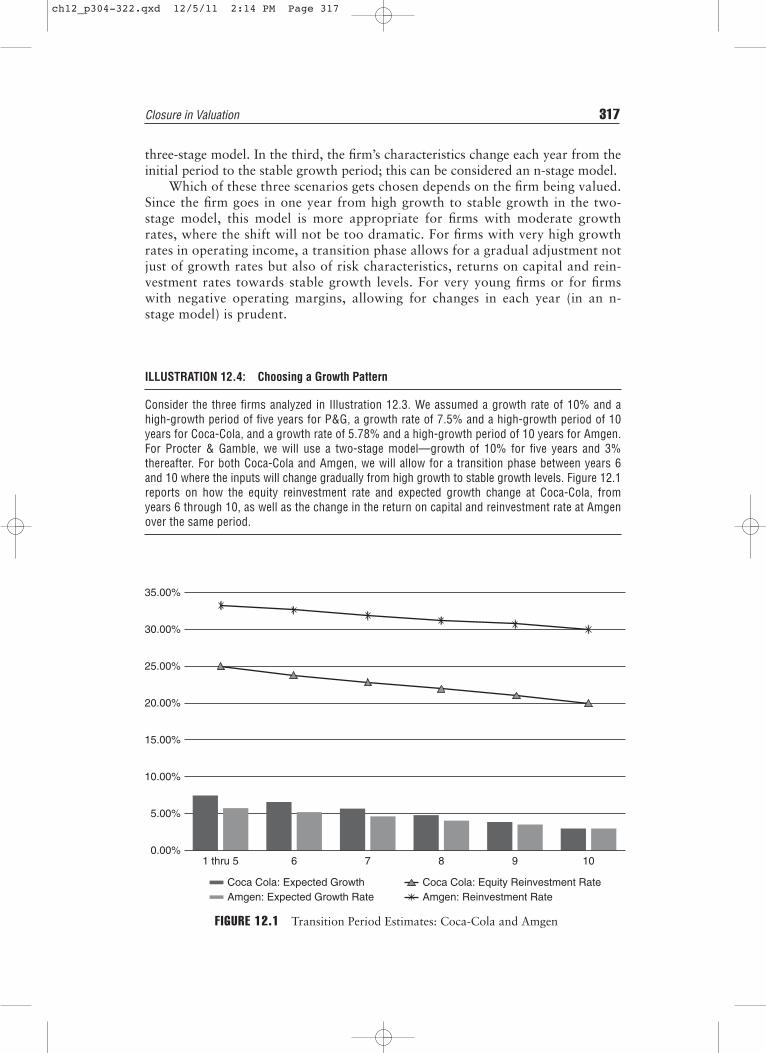
Consider the three firms analyzed in Illustration 12.3. We assumed a growth rate of 10% and ahigh-growth period of five years for P&G, a growth rate of 7.5% and a high-growth period of 10years for Coca-Cola, and a growth rate of 5.78% and a high-growth period of 10 years for Amgen.For Procter & Gamble, we will use a two-stage model—growth of 10% for five years and 3%thereafter. For both Coca-Cola and Amgen, we will allow for a transition phase between years 6and 10 where the inputs will change gradually from high growth to stable growth levels. Figure 12.1reports on how the equity reinvestment rate and expected growth change at Coca-Cola, fromyears 6 through 10, as well as the change in the return on capital and reinvestment rate at Amgenover the same period.

Closure in Valuation 317

FIGURE 12.1 Transition Period Estimates: Coca-Cola and Amgen

0.00%1 thru 5 6 7 8 9 10

5.00%

10.00%

15.00%

20.00%

25.00%

30.00%

35.00%

Coca Cola: Expected GrowthAmgen: Expected Growth Rate

Coca Cola: Equity Reinvestment RateAmgen: Reinvestment Rate

ch12_p304-322.qxd 12/5/11 2:14 PM Page 317

THE SURVIVAL ISSUE

Implicit in the use of a terminal value in discounted cash flow valuation is the as-sumption that the value of a firm comes from it being a going concern with a per-petual life. For many risky firms, there is the very real possibility that they mightnot be in existence in 5 or 10 years, with volatile earnings and shifting technology.Should the valuation reflect this chance of failure, and, if so, how can the likelihoodthat a firm will not survive be built into a valuation?

Life Cycle and Firm Survival

There is a link between where a firm is in the life cycle and survival. Young firmswith negative earnings and cash flows can run into serious cash flow problems andend up being acquired by firms with more resources at bargain basement prices.Why are young firms more exposed to this problem? The negative cash flows fromoperations, when combined with significant reinvestment needs, can result in arapid depletion of cash reserves. When financial markets are accessible and addi-tional equity (or debt) can be raised at will, raising more funds to meet these fund-ing needs is not a problem. However, when stock prices drop and access to marketsbecomes more limited, these firms can be in trouble.

A widely used measure of the potential for a cash flow problem for firms withnegative earnings is the cash burn ratio, which is estimated as the cash balance ofthe firm divided by its earnings before interest, taxes, depreciation, and amortiza-tion (EBITDA).

Cash burn ratio = Cash balance/EBITDA

318 CLOSURE IN VALUATION: ESTIMATING TERMINAL VALUE

EXTRAORDINARY GROWTH PERIODS WITHOUT A HIGH GROWTH RATE OR A NEGATIVE GROWTH RATE

Can you have extraordinary growth periods for firms that have expectedgrowth rates that are less than or equal to the growth rate of the economy? Theanswer is yes, for some firms. This is because stable growth requires not justthat the growth rate be less than the growth rate of the economy, but that theother inputs into the valuation are also appropriate for a stable growth firm.Consider, for instance, a firm whose operating income is growing at 4 percent ayear but whose current return on capital is 20 percent and whose beta is 1.5.You would still need a transition period where the return on capital declined tomore sustainable levels (say 12 percent) and the beta moved toward 1.

By the same token, you can have an extraordinary growth period, wherethe growth rate is less than the stable growth rate and then moves up to thestable growth rate. For instance, you could have a firm that is expected to seeits earnings grow at 2 percent a year for the next five years (which would bethe extraordinary growth period) and 5 percent thereafter.

ch12_p304-322.qxd 12/5/11 2:14 PM Page 318

where EBITDA is a negative number and the absolute value of EBITDA is used toestimate this ratio. Thus a firm with a cash balance of $1 billion and EBITDA of–$1.5 billion will burn through its cash balance in eight months.

Likelihood of Failure and Valuation

One view of survival is that the expected cash flows that you use in a valuation reflectcash flows under a wide range of scenarios from very good to abysmal and the proba-bilities of the scenarios occurring. Thus, the expected value already has built into it thelikelihood that the firm will not survive. Any market risk associated with survival orfailure is assumed to be incorporated into the cost of capital. Firms with a high likeli-hood of failure will therefore have higher discount rates and lower present values.

Another view of survival is that discounted cash flow valuations tend to have anoptimistic bias and that the likelihood that the firm will not survive is not consideredadequately in the value. With this view, the discounted cash flow value that emergesfrom the analysis in the prior section overstates the value of operating assets and hasto be adjusted to reflect the likelihood that the firm will not survive to deliver its ter-minal value or even the positive cash flows that you have forecast in future years.

Should You or Should You Not Discount Value for Survival?

For firms that have substantial assets in place and relatively small probabilities ofdistress, the first view is the more appropriate one. Attaching an extra discount fornonsurvival is double counting risk.

For younger and smaller firms, it is a tougher call and depends on whether ex-pected cash flows consider the probability that these firms may not make it past thefirst few years. If they do, the valuation already reflects the likelihood that the firmswill not survive past the first few years. If they do not, you do have to discount thevalue for the likelihood that the firm will not survive the near future. One way toestimate this discount is to use the cash burn ratio, described earlier, to estimate aprobability of failure, and adjust the operating asset value for this probability:

Adjusted value = Discounted cash flow value(1 − Probability of distress) + Distressed sale value(Probability of distress)

For a firm with a discounted cash flow value of $1 billion on its assets, a distresssale value of $500 million and a 20 percent probability of distress, the adjustedvalue would be $900 million:

Adjusted value = $1,000(.8) + $500(.2) = $900 million

There are two points worth noting here. It is not the failure to survive per se thatcauses the loss of value but the fact that the distressed sale value is at a discount on theIntrinsic value. The second is that this approach revolves around estimating the proba-bility of failure. This probability is difficult to estimate because it will depend uponboth the magnitude of the cash reserves of the firm (relative to its cash needs) and thestate of the market. In buoyant equity markets, even firms with little or no cash cansurvive because they can access markets for more funds. Under more negative marketconditions, even firms with significant cash balances may find themselves under threat.

The Survival Issue 319

ch12_p304-322.qxd 12/5/11 2:14 PM Page 319

CLOSING THOUGHTS ON TERMINAL VALUE

The role played by the terminal value in discounted cash flow valuations has oftenbeen the source of much of the criticism of the discounted cash flow approach.Critics of the approach argue that too great a proportion of the discounted cashflow value comes from the terminal value and that it is easy to manipulate the ter-minal value to yield any number you want. They are wrong on both counts.

It is true that a large portion of the value of any stock or equity in a businesscomes from the terminal value, but it would be surprising if it were not so. Whenyou buy a stock or invest in the equity in a business, consider how you get your re-turns. Assuming that your investment is a good investment, the bulk of the returnscome not while you hold the equity (from dividends or other cash flows) but whenyou sell it (from price appreciation). The terminal value is designed to capture thelatter. Consequently, the greater the growth potential in a business, the higher theproportion of the value that comes from the terminal value.

Is it easy to manipulate the terminal value? We concede that terminal value is ma-nipulated often and easily, but it is because analysts either use multiples to get thesevalues or because they violate one or both of two basic propositions in stable growthmodels. One is that the growth rate cannot exceed the growth rate of the economy.

320 CLOSURE IN VALUATION: ESTIMATING TERMINAL VALUE

ESTIMATING THE PROBABILITY OF DISTRESS

There are two ways in which we can estimate the probability that a firm willnot survive. One is to draw on the past, look at firms that have failed, com-pare them to firms that did not, and look for variables that seem to set themapart. For instance, firms with high debt ratios and negative cash flows fromoperations may be more likely to fail than firms without these characteristics.In fact, you can use statistical techniques such as probits to estimate the prob-ability that a firm will fail. To run a probit, you would begin, for instance,with all listed firms in 1990 and their financial characteristics, identify thefirms that failed during the 1991–1999 time period and then estimate theprobability of failure as a function of variables that were observable in 1990.The output, which resembles regression output, will then let you estimate theprobability of default for any firm today.

The other way of estimating the probability of default is to use the bondrating for the firm, if it is available. For instance, assume that Tesla Motorshas a B rating. An empirical examination of B-rated bonds over the past fewdecades reveals that the likelihood of default with this rating is 36.80 per-cent.5 While this approach is simpler, it is limiting insofar as it can be usedonly for rated firms, and it assumes that the standards used by ratings agen-cies have not changed significantly over time.

5Professor Altman at NYU’s Stern School of Business estimates these probabilities as part ofan annual series that he updates. The latest version is available from the Stern School ofBusiness working paper series.

ch12_p304-322.qxd 12/5/11 2:14 PM Page 320

The other is that firms have to reinvest in stable growth to generate the growth rate.In fact, as we showed earlier in the chapter, it is not the stable growth rate that drivesvalue as much as what we assume about excess returns in perpetuity. When excess re-turns are zero, changes in the stable growth rate have no impact on value.

CONCLUSION

The value of a firm is the present value of its expected cash flows over its life. Sincefirms have infinite lives, you apply closure to a valuation by estimating cash flowsfor a period and then estimating a value for the firm at the end of the period—a ter-minal value. Many analysts estimate the terminal value using a multiple of earningsor revenues in the final estimation year. If you assume that firms have infinite lives,an approach that is more consistent with discounted cash flow valuation is to as-sume that the cash flows of the firm will grow at a constant rate forever beyond apoint in time. When the firm that you are valuing will approach this growth rate,which you label a stable growth rate, is a key part of any discounted cash flow valu-ation. Small firms that are growing fast and have significant competitive advantagesshould be able to grow at high rates for much longer periods than larger and moremature firms, without these competitive advantages. If you do not want to assumean infinite life for a firm, you can estimate a liquidation value based on what otherswill pay for the assets that the firm has accumulated during the high-growth phase.

QUESTIONS AND SHORT PROBLEMS

In the problems following, use an equity risk premium of 5.5 percent if none isspecified.1. Ulysses Inc. is a shipping company with $100 million in earnings before interest

and taxes that is expected to have earnings growth of 10% for the next fiveyears. At the end of the fifth year, you estimate the terminal value using a multi-ple of 8 times operating income (which is the average for the sector).a. Estimate the terminal value of the firm.b. If the cost of capital for Ulysses is 10%, the tax rate is 40%, and you expect

the stable growth rate to be 5%, what is the return on capital that you are as-suming in perpetuity if you use a multiple of 8 times operating income.

2. Genoa Pasta manufactures Italian food products and currently earns $80 millionin earnings before interest and taxes. You expect the firm’s earnings to grow 20percent a year for the next six years and 5% thereafter. The firm’s current after-tax return on capital is 28%, but you expect it to be halved after the sixth year.If the cost of capital for the firm is expected to be 10% in perpetuity, estimatethe terminal value for the firm. (The tax rate for the firm is 40%.)

3. Lamps Galore Inc. manufactures table lamps and earns an after-tax return oncapital of 15% on its current capital invested (which is $100 million). You ex-pect the firm to reinvest 80% of its after-tax operating income back into thebusiness for the next four years and 30% thereafter (the stable growth period).The cost of capital for the firm is 9%.a. Estimate the terminal value for the firm (at the end of the fourth year).b. If you expected the after-tax return on capital to drop to 9% after the fourth

year, what would your estimate of terminal value be?

Questions and Short Problems 321

ch12_p304-322.qxd 12/5/11 2:14 PM Page 321

4. Bevan Real Estate Inc. is a real estate holding company with four properties.You estimate that the income from these properties, which is currently $50 mil-lion after taxes, will grow 8% a year for the next 10 years and 3% thereafter.The current market value of the properties is $500 million, and you expect thisvalue to appreciate at 3% a year for the next 10 years.a. Estimate the terminal value of the properties, based on the current market

value and the expected appreciation rate in property values.b. Assuming that your projections of income growth are right, what is the ter-

minal value as a multiple of after-tax operating income in the tenth year?c. If you assume that no reinvestment is needed after the tenth year, estimate the

cost of capital that you are implicitly assuming with your estimate of the ter-minal value.

5. Latin Beats Corporation is a firm that specializes in Spanish music and videos. Inthe current year, the firm reported $20 million in after-tax operating income,$15 million in capital expenditures, and $5 million in depreciation. The firm ex-pects all three items to grow at 10% for the next five years. Beyond the fifthyear, the firm expects to be in stable growth and grow at 4% a year in perpetu-ity. You assume that earnings, capital expenditures, and depreciation will growat 4% in perpetuity and that your cost of capital is 12%. (There is no workingcapital.)a. Estimate the terminal value of the firm.b. What reinvestment rate and return and capital are you implicitly assuming in

perpetuity when you do this?c. What would your terminal value have been if you had assumed that capital

expenditures offset depreciation in stable growth?d. What return on capital are you implicitly assuming in perpetuity when you

set capital expenditures equal to depreciation?6. Crabbe Steel owns a number of steel plants in Pennsylvania. The firm reported

after-tax operating income of $40 million in the most recent year on capital in-vested of $400 million. The firm expects operating income to grow 7% a yearfor the next three years, and 3% thereafter. a. If the firm’s cost of capital is 10% and you expect the firm’s current return on

capital to continue in perpetuity, estimate the value at the end of the thirdyear.

b. If you expect operating income to stay fixed after year 3 (what you earn inyear 3 is what you will earn every year thereafter), estimate the terminalvalue.

c. If you expect operating income to drop 5% a year in perpetuity after year 3,estimate the terminal value.

7. How would your answers to the preceding problem change if you were told thatthe cost of capital for the firm is 8%?

322 CLOSURE IN VALUATION: ESTIMATING TERMINAL VALUE

ch12_p304-322.qxd 12/5/11 2:14 PM Page 322