9832 IEEE TRANSACTIONS ON GEOSCIENCE AND REMOTE SENSING, VOL. 57, NO. 12, DECEMBER 2019

Cloud Deep Networks for HyperspectralImage Analysis

Juan Mario Haut , Student Member, IEEE, Jose Antonio Gallardo ,Mercedes E. Paoletti , Student Member, IEEE, Gabriele Cavallaro , Member, IEEE,

Javier Plaza , Senior Member, IEEE, Antonio Plaza , Fellow, IEEE,and Morris Riedel, Member, IEEE

Abstract— Advances in remote sensing hardware have ledto a significantly increased capability for high-quality dataacquisition, which allows the collection of remotely sensed imageswith very high spatial, spectral, and radiometric resolution. Thistrend calls for the development of new techniques to enhancethe way that such unprecedented volumes of data are stored,processed, and analyzed. An important approach to deal withmassive volumes of information is data compression, related tohow data are compressed before their storage or transmission.For instance, hyperspectral images (HSIs) are characterized byhundreds of spectral bands. In this sense, high-performancecomputing (HPC) and high-throughput computing (HTC) offerinteresting alternatives. Particularly, distributed solutions basedon cloud computing can manage and store huge amounts of datain fault-tolerant environments, by interconnecting distributedcomputing nodes so that no specialized hardware is needed.This strategy greatly reduces the processing costs, making theprocessing of high volumes of remotely sensed data a naturaland even cheap solution. In this paper, we present a new cloud-based technique for spectral analysis and compression of HSIs.Specifically, we develop a cloud implementation of a populardeep neural network for non-linear data compression, knownas autoencoder (AE). Apache Spark serves as the backbone of

Manuscript received January 15, 2019; revised May 4, 2019 andJuly 3, 2019; accepted July 16, 2019. Date of publication August 14, 2019;date of current version November 25, 2019. This work was supported inpart by the Ministerio de Educación (Resolución de 26 de diciembre de2014 y de 19 de noviembre de 2015, de la Secretaría de Estado de Educación,Formación Profesional y Universidades, por la que se convocan ayudas parala formación de profesorado universitario, de los subprogramas de Formacióny de Movilidad incluidos en el Programa Estatal de Promoción del Talento ysu Empleabilidad, and en el marco del Plan Estatal de Investigación Científicay Técnica y de Innovación 2013-2016), in part by the Junta de Extremadura(decreto 14/2018, ayudas para la realización de actividades de investigación ydesarrollo tecnológico, and de divulgación y de transferencia de conocimientopor los Grupos de Investigación de Extremadura) under Grant GR18060,in part by the MINECO Project under Grant TIN2015-63646-C5-5-R, in partby the National Science Foundation under Grant ACI-1548562, and in partby the European Union under Grant 734541-EXPOSURE. (Correspondingauthor: Juan M. Haut)

J. M. Haut, J. A. Gallardo, M. E. Paoletti, J. Plaza, and A. Plaza are withthe Hyperspectral Computing Laboratory, Department of Technology of Com-puters and Communications, Escuela Politécnica, University of Extremadura,10003 Cáceres, Spain (e-mail: juanmariohaut@unex.es; mpaoletti@unex.es;jplaza@unex.es; aplaza@unex.es).

G. Cavallaro is with the Jülich Supercomputing Center, 52428 Jülich,Germany (e-mail: g.cavallaro@fz-juelich.de).

M. Riedel is with the Jülich Supercomputing Center, 52428 Jülich, Germany,and also with the Faculty of Industrial Engineering, Mechanical Engineeringand Computer Science, University of Iceland, 107 Reykjavik, Iceland (e-mail:m.riedel@fz-juelich.de)

Color versions of one or more of the figures in this article are availableonline at http://ieeexplore.ieee.org.

Digital Object Identifier 10.1109/TGRS.2019.2929731

our cloud computing environment by connecting the availableprocessing nodes using a master–slave architecture. Our newlydeveloped approach has been tested using two widely availableHSI data sets. Experimental results indicate that cloud comput-ing architectures offer an adequate solution for managing bigremotely sensed data sets.

Index Terms— Autoencoder (AE), cloud computing, dimen-sionality reduction (DR), high-performance computing (HPC),high-throughput computing (HTC), hyperspectral images (HSIs),speedup.

I. INTRODUCTION

EARTH observation (EO) has evolved dramatically in thelast decades due to the technological advances incor-

porated into remote sensing instruments in the optical andmicrowave domains [1]. With their hundreds of contiguous andnarrow channels within the visible, near-infrared, and short-wave infrared spectral ranges, hyperspectral images (HSIs)have been used for the retrieval of bio-chemical, geo-chemical,and physical parameters that characterize the surface of theearth. These data are now used in a wide range of applications,aimed at monitoring and implementing new policies in thedomain of agriculture, geology, assessment of environmentalresources, urban planning, military/defense, disaster manage-ment, and so on [2]–[4].

Most of the developments carried out over the last decadesin the field of imaging spectroscopy have been achieved viaspectrometers onboard airborne platforms. For instance, theAirborne Visible/Infrared Imaging Spectrometer (AVIRIS) [5]has been dedicated to remote sensing of the earth in alarge number of experiments and field campaigns since thelate 1980s. Other examples of airborne missions include theEuropean Space Agency (ESA)’s Airborne Prism Experiment(APEX) (2011–2016) [6] or the Compact Airborne Spectro-graphic Imager (CASI) [7] (since 1989), among many others.

The vast amount of data collected by airborne platformshas paved the way for EO satellite hyperspectral missions.The Hyperion instrument onboard National Aeronautics andSpace Administration (NASA)’s Earth Observing One (EO-1)spacecraft (2000–2017) [8] and the Compact High ResolutionImaging Spectrometer (CHRIS) on ESA’s Proba-1 microsatel-lite [9] (since 2001) have to be the main sources of space-based HSI data in the last decades. Currently, there are severalHSI missions under development, including the Environmen-tal Mapping and Analysis Program (EnMAP) [10] and the

0196-2892 © 2019 IEEE. Personal use is permitted, but republication/redistribution requires IEEE permission.See http://www.ieee.org/publications_standards/publications/rights/index.html for more information.

HAUT et al.: CLOUD DEEP NETWORKS FOR HSI ANALYSIS 9833

Prototype Research Instruments and Space Mission technologyAdvancement (PRISMA) [11], among others.

The adoption of an open and free data policy by theNASA [12] and, more recently, by ESA’s Copernicus initia-tive (the largest single EO program) [13] is now producingan unprecedented amount of data to the research commu-nity. Even though the Copernicus space component (i.e., theSentinels) has not included a hyperpectral instrument yet(Sentinel-10 is an HSI mission expected to be operationalaround 2025–2030), it has been shown that the vast amount ofopen data currently available calls for re-definition of the chal-lenges within the entire HSI life cycle (i.e., data acquisition,processing, and application phases). It is not by coincidencethat remote sensing data are now described under the big dataterminology, with characteristics such as volume (increasingscale of acquired/archived data), velocity (rapidly growing datageneration rate and real-time processing needs), variety (dataacquired from multiple sources), veracity (data uncertainty/accuracy), and value (extracted information) [14], [15].

In this context, traditional processing methods, such asdesktop approaches (i.e., MATLAB, R, SAS, and ENVI), offerlimited capabilities when dealing with such large amounts ofdata, especially regarding the velocity component (i.e., thedemand for real-time applications). Despite modern desktopcomputers and laptops are becoming increasingly more pow-erful, with multi-core and many-core capabilities, includinggraphics processing units (GPUs), the limitations in terms ofmemory and core availability currently limit the processing oflarge HSI data archives. Therefore, the use of highly scalableparallel/distributed architectures (such as GPUs, clusters [16],grids [17], or clouds [18], [19]) is a mandatory solutionto improve the access to and the analysis of such greatamount of complex data, in order to provide decision-makerswith clear, timely, and useful information [20], [21]. In thiscontext, parallel and distributed computing approaches canbe categorized into high-performance computing (HPC) orhigh-throughput computing (HTC) solutions. Contrary to anHPC system [22] (generally, a supercomputer that includes amassive number of processors connected through a fast ded-icated network, i.e., a cluster), an HTC system (for instance,a grid) is more focused on the execution of independentand sequential jobs that can be individually scheduled onmany different computing resources, regardless of how fastan individual job can be completed. Cloud computing is thenatural evolution of grid computing, adopting its backboneand infrastructure [19] but delivering computing resources asa service over the network connection [23]. In other words,the cloud moves desktop and laptop computing (via the Inter-net) to a service-oriented platform using large remote serverclusters and massive storage to data centers. In this scenario,computing relies on sharing a pool of physical and/or virtualresources rather than on deploying local or personal hardwareand software. The process of virtualization has enabled thecost-effectiveness and simplicity of cloud computing solu-tions [24] (i.e., it exempts users from the need to purchase andmaintain complex computing hardware), such as infrastructureas a service (IaaS), platform as a service (PaaS), or softwareas a service (SaaS). Several cloud computing resources are

currently available commercially on a pay as you go modelfrom providers, such as Amazon Web Services (AWS) [25],Microsoft Azure [26], and Google’s Compute Engine [27].

Cloud computing infrastructures can rely on several com-puting frameworks that support the processing of largedata sets in a distributed environment. For example, theMapReduce model [28] is the basis of a large number ofopen-source implementations. The most popular ones areApache Hadoop [29] and its variant, Apache Spark [30](an in-memory computing framework). Despite the recentadvances in cloud computing technology, not enough effortshave been devoted to exploiting cloud computing infrastruc-tures for the processing of HSI data. However, cloud comput-ing offers a natural solution for the processing of large HSIdatabases, as well as an evolution of the previously developedtechniques for other kinds of computing platforms, mainly dueto the capacity of cloud computing to provide Internet-scale,service-oriented computing [31]–[33].

In this paper, we focus on the problem of howto develop scalable data analysis and compressiontechniques [4], [34]–[36] with the goal of facilitatingthe management of remotely sensed HSI data. In thissense, deep learning (DL) methods based on neural networkarchitectures have gained significant interest in HSI imageanalysis and processing [37] due to the flexibility of theirarchitectures, their learning models, and the amount of tasksthat they can perform [38]. As a result, dimensionalityreduction (DR) of HSIs is a fundamental pre-processingstep that is applied before many data transfer, store, andprocessing operations. On the one hand, when HSI data areefficiently compressed, they can be handled more efficientlyonboard satellite platforms with limited storage and downlinkbandwidth. On the other hand, since HSI data live primarilyin a subspace [39], a few informative features can be extractedfrom the hundreds of highly correlated spectral bands thatcomprise HSI data [40] without significantly affecting thedata quality (lossy compression of HSIs can still retaininformative data for the subsequent processing steps).

Specifically, this paper develops a new cloud implemen-tation of HSI data compression based on neural networks.As in [41], we adopt the Apache Spark framework as well asa map-reduce methodology [24] to carry out our implemen-tation. In addition, we address the DR problem using a non-linear deep autoencoder (AE) neural network instead of thestandard linear principal component analysis (PCA) algorithm.In fact, we implement a new scalable cloud implementationof the neural model proposed in [42], which is character-ized by its flexibility to perform different tasks beyond DR,such as classification [42] or spectral unmixing [43], andtherefore, the proposed methodology can be easily adaptedto perform different tasks. Focusing on DR, the performanceof our newly proposed cloud-based AE is validated usingtwo widely available and known HSI data sets. Our exper-imental results show that the proposed implementation caneffectively exploit cloud computing technology to efficientlyperform non-linear compression of large HSI data sets whileaccelerating significantly the processing time in a distributedenvironment.

9834 IEEE TRANSACTIONS ON GEOSCIENCE AND REMOTE SENSING, VOL. 57, NO. 12, DECEMBER 2019

The remainder of this paper is organized as follows.Section II provides an overview of the theoretical and opera-tional details of the considered AE neural network for HSIdata compression and the considered optimization method.Section III presents our cloud-distributed AE network forHSI data compression, describing the details of the networkconfiguration and the distributed implementation. Section IVevaluates the performance of the proposed approach usingtwo widely available HSI data sets, considering the qualityof the compression and signal reconstruction and also thecomputational efficiency of the implementation in a real cloudenvironment. Finally, Section V concludes this paper, summa-rizing the obtained results and suggesting some future researchdirections.

II. BACKGROUND

HSI data are characterized by their intrinsically complexspectral characteristics, where samples of the same classexhibit high variability due to data acquisition factors oratmospheric and lighting interferers. DR and feature extrac-tion (FE) methods are fundamental tools for the extraction ofdiscriminative features that reduce the intra-class variabilityand inter-class similarity [44] present in the HSI data sets.Furthermore, by reducing the high spectral dimensionality ofHSIs, these methods are able to alleviate the curse of dimen-sionality [45], which makes HSI data difficult to interpret bysupervised classifiers due to the Hughes phenomenon [46].

Several methods have been developed to perform DR andFE from HSIs, For instance, Kang et al. [47] proposed adecolorization method to reduce the spectral dimensionalityof HSI scenes, preserving most of the information containedin them. In [48], they adopted DR methods with data filtering,implementing image fusion and recursive filtering (IFRF)to preserve the physical meaning of the spectral pixels.In [49], they implemented morphological attribute thinningand thickening (attribute filtering) to perform advanced FEfor HSI interpretation. Other interesting DR and FE methodsare the independent component analysis (ICA) [50], [51]or the maximum noise fraction (MNF) [52], [53], beingPCA [54]–[56] one of the most widely used methods forFE purposes. This unsupervised, linear algorithm reducesthe original high-dimensional and correlated feature spaceto a lower dimensional space of uncorrelated factors [alsocalled principal components (PCs)] by applying an orthogonaltransformation through a projection matrix, which makes ita simple yet efficient algorithm. However, PCA is restrictedto a linear map projection and is not able to learn non-linear transformations. In this context, auto-associative1 neuralnetworks, such as AEs [57], offer a more flexible architecturefor FE and DR purposes, managing the non-linearities ofthe data through an architecture made up of stacked layersand non-linear activation functions [called stacked AE (SAE)]that can provide more detailed data representations from theoriginal input image (one per layer), which can be easilyreused by other HSI processing methods [42], [43].

1Auto-associative networks are those whose inputs can be inferred from theoutputs. The proposed implementation of a non-linear AE belongs to this kindof networks.

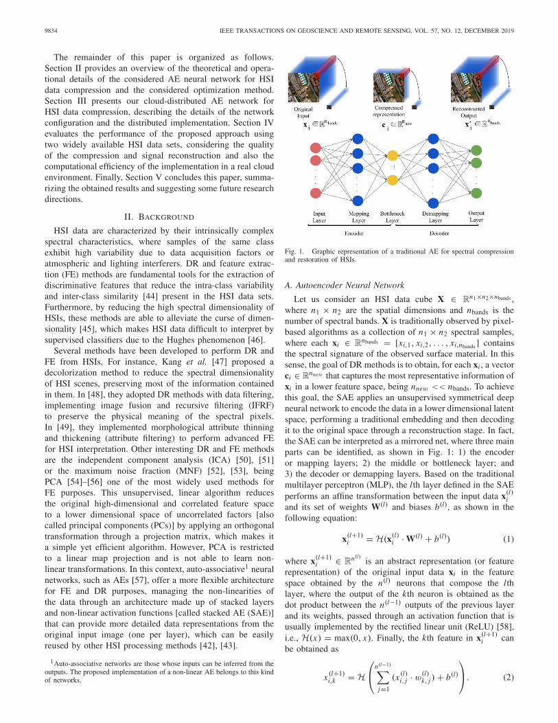
Fig. 1. Graphic representation of a traditional AE for spectral compressionand restoration of HSIs.

A. Autoencoder Neural Network

Let us consider an HSI data cube X ∈ Rn1×n2×nbands ,

where n1 × n2 are the spatial dimensions and nbands is thenumber of spectral bands. X is traditionally observed by pixel-based algorithms as a collection of n1 × n2 spectral samples,where each xi ∈ R

nbands = [xi,1, xi,2, . . . , xi,nbands ] containsthe spectral signature of the observed surface material. In thissense, the goal of DR methods is to obtain, for each xi , a vectorci ∈ R

nnew that captures the most representative information ofxi in a lower feature space, being nnew << nbands. To achievethis goal, the SAE applies an unsupervised symmetrical deepneural network to encode the data in a lower dimensional latentspace, performing a traditional embedding and then decodingit to the original space through a reconstruction stage. In fact,the SAE can be interpreted as a mirrored net, where three mainparts can be identified, as shown in Fig. 1: 1) the encoderor mapping layers; 2) the middle or bottleneck layer; and3) the decoder or demapping layers. Based on the traditionalmultilayer perceptron (MLP), the lth layer defined in the SAEperforms an affine transformation between the input data x(l)

iand its set of weights W(l) and biases b(l), as shown in thefollowing equation:

x(l+1)i = H(x(l)

i ·W(l) + b(l)) (1)

where x(l+1)i ∈ R

n(l)is an abstract representation (or feature

representation) of the original input data xi in the featurespace obtained by the n(l) neurons that compose the lthlayer, where the output of the kth neuron is obtained as thedot product between the n(l−1) outputs of the previous layerand its weights, passed through an activation function that isusually implemented by the rectified linear unit (ReLU) [58],i.e., H(x) = max(0, x). Finally, the kth feature in x(l+1)

i canbe obtained as

x (l+1)i,k = H

⎛⎝n(l−1)�

j=1

(x (l)i, j ·w(l)

k, j )+ b(l)

⎞⎠. (2)

HAUT et al.: CLOUD DEEP NETWORKS FOR HSI ANALYSIS 9835

With this in mind, the SAE applies two main processingsteps to each input sample xi . The first one, known as codingstage, performs the embedding of the data, mapping it fromR

nbands space to Rnnew latent space, that is, the nencoder layers

of the encoder map their input data to a projected representa-tion following (1) and (2) until reaching the bottleneck layer.As a result, the bottleneck layer contains the projection of eachxi ∈ R

nbands in its latent space, defined by its nnew neurons,ci ∈ R

nnew . As a result, the SAE allows to generate compressed(nnew < nbands), extended (nnew > nbands), or even equally(nnew = nbands) dimensional representations, depending onthe final dimension of the code vector ci .

The second stage performs the opposite operation, i.e., thedecoding, where the network tries to recover the originalinformation, obtaining an approximate reconstruction of theoriginal input vector [59]. In this case, the ndecoder layersof the decoder demap the code vector ci until reaching theoutput layer, where a reconstructed sample x�i is obtained.Equation (3) shows an overview of the encoding–decodingprocess followed by the SAE:ci ← For l in nencoder: x(l+1)

i = H�x(l)

i ·W(l) + b(l)�x�i ← For ll in ndecoder: c(ll+1)

i = H�c(ll)

i ·W(ll) + b(ll)�. (3)

In order to obtain a lower dimensional (but more discrimina-tive) representation of the input data, the network parametersare iteratively adjusted in an unsupervised fashion, wherethe optimizer minimizes the reconstruction error between theinput data at the encoding stage, xi , and its reconstruction atthe end of the decoding stage, x�i . This error function, givenby (4), is usually implemented in the form of a mean squarederror (MSE)

E(X) = min � X− X� �2= minn1·n2�i=1

� xi − x�i �2 . (4)

B. Broyden–Fletcher–Goldfarb–Shanno AlgorithmAfter describing the operational procedure of SAEs, it is

now important to observe the network optimization process.As any artificial neural network with backpropagation, theoptimizer tries to find the set of parameters (synaptic weightsand biases) that, for a given network architecture, minimizethe error function E(X) defined by (4). This function evaluateshow well the neural network fits the data set X and dependson the adaptative and learnable parameters of the network,which can be denoted as W , so E(X,W). As E(X,W) isnon-linear, its optimization must be carried out iteratively,reducing its value until an adequate stopping criterion isreached. In this sense, standard optimizers back-propagate theerror signal through the network architecture calculating, foreach learnable parameter, the gradient of the error, i.e., thedirection and displacement that the parameter must undergoin order to minimize the final error (also interpreted as theimportance of that parameter when obtaining the final error).Mathematically, the updating of W in the tth epoch can becalculated by

Wt+1 = Wt +�Wbeing �W = μt · pt (5)

where μt and pt are the learning rate (a positive scalar) andthe descent search direction, respectively [60]. The main goalof any optimizer is to obtain the correct pt in order to descendproperly in the error function until the minimum is reached.

As opposed to standard optimizers, traditional Newton-based methods determine the descent direction pt usingthe second derivative information contained into the Hessianmatrix, rather than just the gradient information, thus stabiliz-ing the process

Ht · pt = −∇E(X,Wt )

pt = −H−1t · ∇E(X,Wt )

Wt+1 = Wt − μt ·H−1t · ∇E(X,Wt ) (6)

where ∇E(X,Wt ) is the gradient of the error function eval-uated with the network’s parameters at the tth epoch, Wt ,and Ht and H−1

t are, respectively, the Hessian matrix and itsinverse obtained at the tth epoch. However, these methodsobtain the Hessian matrix and its inverse at each epoch,which is quite expensive to compute, requiring a large amountof memory. Instead of that, the Broyden–Fletcher–Goldfarb–Shanno (BFGS) method [61] performs an estimation of howthe Hessian matrix has changed in each epoch, obtaining anapproximation (instead of the full matrix) that is improvedfor every epoch. In fact, as any algorithm of the family ofmultivariate minimization quasi-Newton methods, the BFGSalgorithm modifies the last expression of (6) as follows:

Wt+1 =Wt − μt ·Gt · ∇E(X,Wt ) (7)

where Gt is the inverse Hessian approximation matrix (usually,when t = 0 the initial approximation matrix is the identitymatrix, G0 = I). This Gt is updated at each epoch by meansof an update matrix

Gt+1 = Gt + Ut . (8)

However, such an update needs to comply with the quasi-Newton condition, which is described next. Assuming thatE(X,W) is continuous for Wt and Wt+1 (with gradientsgt = ∇E(X,Wt ) and gt+1 = ∇E(X,Wt+1), respectively)and the Hessian H is constant, then (9) is satisfied

qt ≡ gt+1 − gt and pt ≡Wt+1 −Wt

Secant condition on the Hessian: qt = H · pt

Secant condition on the inverse: H−1 · qt = pt . (9)

Since G = H−1, the last expression in (9) can be modified toG · qt = pt , so the approximation matrix G can be obtained(at each epoch t) as a combination of the linearly indepen-dent directions and their respective gradients. Following theDavidon–Fletcher–Powell (DFP) rank 2 formula [62], G canbe updated using

Gt+1 = Gt + pt · p�tp�t · qt

−Gt · qt · q�tq�t ·Gt · qt

·Gt . (10)

Finally, the BFGS method updates its approximation matrixby computing the complementary formula of the DFP method,

9836 IEEE TRANSACTIONS ON GEOSCIENCE AND REMOTE SENSING, VOL. 57, NO. 12, DECEMBER 2019

Algorithm 1 BFGS Algorithm1: procedure BFGS(Wt : current parameters of the neural

network, E(X,W): Error function, Gt : current approx-imation to the Hessian)

2: gt = ∇E(X,Wt )3: pt = −Gt · gt

4: Wt+1 =Wt + μt · pt μt by linear search5: gt+1 = ∇E(X,Wt+1)6: qt = gt+1 − gt

7: pt =Wt+1 −Wt

8: A =

1+ q�t ·Gt ·qt

q�t ·pt

·

pt ·p�tp�t ·qt

9: B = pt ·q�t ·Gt+Gt ·qt ·p�t

q�t ·pt10: Gt+1 = Gt + A− B

return Wt+1, Gt+111: end procedure

changing G by H and pt by qt , and therefore, (10) is finallymodified as follows:

Ht+1 = Ht + qt · q�tq�t · pt

−Ht · pt · p�tp�t ·Ht · pt

·Ht . (11)

As the BFGS method intends to compute the inverse of H andG = H−1, it inverts (11) to analytically obtain the final updateof the approximation matrix

Gt+1 = Gt +�

1+ q�t ·Gt · qt

q�t · pt

�·�

pt · p�tp�t · qt

�

− pt · q�t ·Gt +Gt · qt · p�tq�t · pt

. (12)

Algorithm 1 provides a general overview of how theBFGS method works in one epoch. As shown in line 4 ofAlgorithm 1, as opposed to most optimization algorithms, thelearning rate is inferred by performing a linear search insteadof using an input parameter. A weakness of BFGS is that itrequires the computation of the gradient on the full data set,consuming a large amount of memory to properly run theoptimization. Considering the dimensionality of HSIs, we canconclude that this method is not able to scale with the numberof samples [63]. In order to overcome this limitation, and withthe aim of speeding up the computation of both the forward(affine transformations) and backward (optimizer) steps of theAE for DR of HSIs, in Section III, we develop a distributedsolution for cloud computing environments.

III. PROPOSED IMPLEMENTATION

A. Distributed FrameworkWe have developed a completely new distributed AE for

HSI data analysis2 that follows the diagram shown in Fig. 2,where it is shown that the proposed cloud-based neural modelhas been implemented as a master–slave, multi-node environ-ment. In this context, two problems have been specificallyaddressed in this paper: 1) the computing engine and 2) thedistributed programming model over the cloud architecture.

2Code available on: https://github.com/jgallardst/cloud-nn-hsi

Fig. 2. Diagram summarizing the overall framework of the proposed cloudimplementation, where the master node takes the HSI data and partitions itbetween the different workers’ nodes, which apply the tasks extracted fromthe graph of transformations, executing the forward and backward steps overtheir data. The obtained gradients are collected and pooled by the masternode, which transmits the final gradient to the neural models stored by eachworker node.

Regarding the first problem, our distributed implementation ofthe network model is run on top of a standalone Spark cluster,due to its capacity to provide fast processing of large datavolumes on distributed platforms, in addition to fault tolerance.Furthermore, the Spark cluster is characterized by a master–slave architecture, which makes it very flexible. Specifically,a Spark cluster is formed by a master node, which manageshow the resources are used and distributed in the cluster byhosting a Java virtual machine (JVM) driver, and the scheduler,which distributes the tasks between the execution nodes andN worker nodes (which can be more than one per node) thatexecute the program tasks by creating a Java distributed agent,called executor (where tasks are computed), and store the datapartitions (see Fig. 3).

In relation to the second point, the adopted programmingmodel to perform the implementation of the distributed AEis based on organizing the original HSI data in tuples orkey/value pairs, in order to apply the MapReduce model [41],which divides the data processing task into two distributedoperations: 1) mapping, which processes a set of data tuples,generating intermediate key–value pairs and 2) reduction,which gathers all the intermediate pairs obtained by themapping to generate the final result. In order to achievethis behavior, data information in Spark is abstracted andencapsulated into a fault-tolerant data structure called ResilientDistributed data set (RDD). These RDDs are organized asdistributed collections of data, which are scattered by Sparkacross the worker nodes when they are needed on the succes-sive computations, being persisted in the memory of the nodesor on the disk. This architecture allows for the parallelizationof the executions, achieved by performing MapReduce tasksover the RDDs on the nodes. Moreover, two basic operationscan be performed on an RDD: 1) the so-called transformationsthat are based on applying an operation to every row on apartition, resulting in another RDD and 2) actions that retrievea value or a set of values that can be both RDD data or theresult of an operation where some RDD data are involved.Operations are queued until an action is called; the needed

HAUT et al.: CLOUD DEEP NETWORKS FOR HSI ANALYSIS 9837

Fig. 3. Graphic representation of a generic Spark cluster, which is composedby one client node and N worker nodes, where in each node, several executorJVMs are running in parallel over several data partitions.

transformations are placed into a dependence graph, whereeach node is a job stage, following a lazy execution paradigm.This means that operations are not performed until they arereally needed, avoiding the repetition of a single operationmore than once.

In order to enable a simple and easy mechanism for man-aging large data sets, the Spark environment provides anotherlevel of abstraction that uses the concept of Dataframe. TheseDataframes allow data to be organized on named columns,being easier to manipulate (as in relational tables, columnscan be accessed by the column name instead of by the index).With this in mind, the Spark standalone cluster functionalitycan be summarized as follows.

1) The master node (also called driver node) creates andmanages the Spark driver (see Fig. 3), a Java processthat contains the SparkContext of the application.

2) The driver context performs the data partitioning andparallelization between the worker nodes, assigning toeach one a number of partitions, which depends on twomain aspects: the block size and the way that the dataare stacked. Also, the driver creates the executors on theworker nodes, which store data partitions on the workernode and perform tasks on them.

3) When an action is called, a job is launched and themaster coordinates how the associated tasks are dis-tributed into the different executors. In order to reducethe data exchanging time, the Spark driver attempts toperform “smart” task allocations so that there are morepossibilities to assign a task to the executor, located inthe worker where the data partition used by the task toperform the operation has been allocated.

4) When all the tasks on a given stage are finished,the Scheduler allocates another stage of the job (if itwas a transformation) or retrieves the final output (if itwas an action).

Algorithm 2 Iterative Process1: procedure SPARK FLOW

2: Parti tioned Data← Spark.parallelizeData()3: t ← 04: while t < niterat ions do5: broadcast Output Data().6: foreach parti tion ∈ Parti tioned Data do7: Parti tioned Data.applyTask().8: end for9: retrieveOutput Data().

10: t ← t + 111: end while12: end procedure

Algorithm 2 shows a general overview of how our algorithmis pipelined in the considered Spark cluster.

B. Cloud Autoencoder Pipeline Implementation:Training and Optimization Process

This section describes in detail the full distributed trainingprocess, from the parallelization of HSI data across nodes tothe intrinsic logic of each training step, explaining the benefitsof our distributed training algorithm. Fig. 4 shows a generaloverview of the full data pipeline developed in this paper.

In the beginning, the original 3-D HSI data cube X ∈R

n1×n2×nbands , where n1×n2 are the spatial dimensions (heightand width) and nbands is the spectral dimension given bythe number of spectral channels, is reshaped into an HSImatrix X ∈ R

npixels×nbands , where npixels = n1 × n2, i.e., eachrow collects a full spectral pixel, being each column thecorresponding value in the spectral band. This matrix X isread by the Spark Driver, which collects the original HSI dataand partitions it into P smaller subsets that are delivered tothe worker nodes in parallel. These workers store the obtainedpartitions on their local disks. In this sense, each data partitioncomposes an RDD.

It must be noted that complex neural network topologiesderive on greedy RAM memory usage on the driver node.Since Spark transformations apply an operation to every row ofthe RDD, the fewer the number of rows, the fewer the numberof operations that must be carried out. In order to improvethe computation of the distributed model, a blocksize (BS)hyperparameter is provided, with the aim of indicating howmany pixels should be stacked into a single row in orderto compute them together. With this observation in mind,the pth data partition (with p = 1, . . . , P) can be seen asa 2-D matrix (p)D ∈ R

nrows×(BS·nbands) composed by nrowsrows, where each one stores BS concatenated spectral pixels,i.e., (p)d j ∈ R

(BS·nbands) = [xi , xi+1, . . . , xi+BS]. In the end,each data partition (p)D stores BS·nrows pixels. The resultingpartitions are then distributed across the worker nodes. Suchdistribution allows the executors, located in each worker node,to apply the subsequent tasks to those partitions that eachworker receives.

After distributing the data into RDDs, a distributed dataanalysis process begins prior to the application of neural

9838 IEEE TRANSACTIONS ON GEOSCIENCE AND REMOTE SENSING, VOL. 57, NO. 12, DECEMBER 2019

Fig. 4. Data pipeline of our distributed AE, where the input HSI cube is firstreshaped into a matrix and then split into several partitions allocated into theSpark worker nodes, composed by several rows where each one contains BSspectral pixels. These data partitions are then duplicated in order to obtainthe input network data and the corresponding output network data. The AEis then executed and, for each iteration t , the gradients are collected by theSpark driver, which calculates the final gradient and performs the optimizationwith the L-BFGS algorithm. The updated weights are finally broadcasted toeach neural model contained in the cluster.

network-based processing. In the first step, the data containedin each partition (p)D are scaled in a distributed way, takingadvantage of the cloud architecture and the available paral-lelization of resources. In this sense, each partition’s row (p)d j

(and, internally, each pixel contained within) is transformedbased on the global maximum and minimum features (xmaxand xmin) of the whole image X, and the column localmaximum and minimum features [(p)dmax and (p)dmin] of thepth partition where the data are allocated

(p)d j =(p)d j −(p) dmin

(p)dmax −(p) dmin(p)d j = (p)d j · (xmax − xmin)+ xmin. (13)

Once the HSI data have been split into partitions and scaled,the next step consists of the application of the AE model.The proposed AE is composed of five layers, as summarizedin Table I. These layers are: l(1), the input layer that receivesthe spectral signature contained in each pixel xi of X (i.e., therows of the distributed partitions), composed by as many

TABLE I

TOPOLOGY OF THE PROPOSED AE NEURALNETWORK FOR HSI ANALYSIS

neurons as spectral bands; l(2), l(3), and l(4), the hidden AElayers, and l(5), the output layer that obtains the reconstructedsignature x�i , composed also by as many neurons as spectralbands.

With the topology described in Table I in mind, the encoderpart is composed by l(1), l(2), and l(3), which performs themapping from the original spectral space to the latent spaceof the bottleneck layer l(3). In addition, the decoder part iscomposed by l(3), l(4), and l(5), which performs the demappingfrom the latent space of l(3) to the original spectral space.

At this point, it is interesting to briefly comment theperformance of the AE network. In order to correctly prop-agate the data through the network, from each partition(p)D ∈ R

nrows×(BS·nbands), a matrix of unstacked pixels (p)X ∈R

(BS·nrows)×nbands is extracted, i.e., the BS spectral pixels thatare contained in each (p)d j = [xi , xi+1, . . . , xi+BS] (withj = 1, . . . , nrows and i = 1, . . . , npixels) are each extracted tocreate, one by one, the rows of (p)X, denoted as (p)xk [withk = 1, . . . , (BS · nrows)] in order to determine the level atwhich the AE is working.

Every training iteration t is performed using the traditionalneural network forward–backward procedure, in addition to atree-aggregate operation that computes and sums the execu-tors’ gradients and losses to return a single loss value anda matrix of gradients. Each executor computes its loss byforwarding the input network data (p)X through the AE layersand comparing the l(5) layer’s output vector with the vectorof input features, following (4) and obtaining (at each t) thecorresponding MSE of the partition: (p)MSEt = E((p)X,Wt ).Gradients are then computed by back-propagating the errorsignal through the AE, obtaining for each partition the (p)Gt

matrix at iteration t . Each gradient matrix is reduced in theDriver, which runs the optimizer in order to obtain the finalmatrix �Wt . This matrix indicates how much each neuronweight should be modified before finishing the tth trainingiteration, based on how that neuron impacts the output. Fig. 5shows a graphical overview of the adopted training procedure.

If we denote by P the number of total partitions andby (p)X ∈ R

(BS·nrows)×nbands the pth unstacked partitiondata, composed by (BS × nrows) normalized rows/featurevectors of nbands spectral features, i.e., (p)xk ∈ R

nbands =[(p)xk,1, . . . ,

(p) xk,nbands ], and considering the lth layer of theAE model, composed by n(l)

neurons, its output is denoted by(p)X(l+1) and it is computed by adapting (1) into (14) as thematrix multiplication

(p)X(l+1) = H((p)X(l) ·W(l) + b(l)) (14)

where the meaning of each term is given in the following.1) (p)X(l+1) ∈ R

(BS×nrows)×n(l)neurons is the matrix that rep-

resents the output of the neurons in layer l with size(BS · nrows) × n(l)

neurons, where n(l)neurons is the number of

HAUT et al.: CLOUD DEEP NETWORKS FOR HSI ANALYSIS 9839

Fig. 5. Distributed forward and backward pipelines of the training stage (at iteration t) after unstacking the hyperspectral pixels in each distributed datapartition (each one allocated to a different worker node).

neurons of the lth layer (in the case that l = 5 andn(5)

neurons = nbands).2) (p)X(l) ∈ R

(BS×nrows)×n(l−1)neurons is the matrix that serves

as the input to the lth layer, which contains the(BS·nrows) pixel vectors represented in the feature spaceof the previous layer, defined by n(l−1)

neurons neurons.3) W(l) ∈ R

n(l−1)neurons×n(l)

neurons is the matrix of weights, whichconnects the current n(l)

neurons neurons with the n(l−1)neurons

neurons of the previous layer, and b(l) is the bias ofthe current layer.

4) H is the ReLU activation function, which gives thefollowing non-linear output: ReLU(x) = max(0, x).

After data forwarding, the reconstructed data (p)X� in thepth partition at the tth iteration are compared to the originalinput (p)X by applying the MSE function defined by (4) oneach executor. Executors then retrieve the error computed bytheir carried data, obtaining a value (p)MSEt per partition.Then, the final error is obtained as the mean of all executorerrors, as shown in the following equation:

(p)MSEt = 1

(BS× nrows)

(BS×nrows)�k=1

�(p) xk −(p) x�k �2

MSEt = 1

P

P�p=1

(p)MSEt (15)

where (BS× nrows) is the number of pixels that compose thepth data partition, whereas (p)xk ∈(p) X and (p)x�k ∈(p) X� arethe original input sample and output reconstructed sample inthe pth data partition, respectively. Those partition errors arethen back-propagated to compute the gradient (p)Gt matrix ofeach partition at iteration t . In this sense, for each layer inthe neural model (using the resulting outputs), the impact thateach neuron has on the final error is obtained as the resultof the ReLU’s derivative of every output, which is defined asfollows:

H�(x) =

0, if x ≤ 0

1, if x > 0.(16)

Such impact can be denoted as (p)gLt = [(p)g(1)

t , . . . ,(p) g(5)t ],

where the lth element (p)g(l)t stores the impact of the n(l)

neurons

allocated into the lth layer of the network.The gradient of each partition, (p)Gt , is then computed by

applying the double-precision general matrix to matrix multi-plication (DGEMM) operation where, given three input matri-ces (A, B, and C) and two constants (α and β), the obtainedresults are calculated by (17) and stored in C

C = α ∗ A ∗ B+ β ∗ C. (17)

DGEMM is performed to compute the entire gradient matrixin parallel, instead of computing each layer gradient vectorsseparately. This allows us to make neural computations fasterand efficient in terms of reducing power consumption. In thissense, each item of (17) has been replaced by the followingparameters.

1) α = (1/nbands) is a parameter regularizer.2) A =(p) X is the input data partition matrix.3) B =(p) gL

t is the matrix representing the impact of eachneuron on every layer of the neural network.

4) β = 1 is also a parameter regularizer. As C should beunchanged, it has been set to 1.

5) C =(p) Gt−1 is initially the older gradient matrix ofthe pth partition. After the updates resulting from theDGEMM operation, the current gradient (p)Gt is storedon C.

Finally, the gradient matrix Gt of the whole network iscomputed as the average of the sum of all partition’s gradi-ents: (p)Gt . The entire training process on each data partitionis graphically shown in Fig. 5.

The final optimization step is performed locally on themaster node using a variant of the BFGS algorithm, calledlimited BFGS (L-BFGS). Since BFGS needs a huge amountof memory for the computation of the matrices, L-BFGS limitsthe memory usage, so it fits better into our implementation.The optimizer uses the computed gradients and a step-sizeprocedure to get closer to a minimum of (4). The procedureis repeated until a desired number of iterations, niterations,is reached.

9840 IEEE TRANSACTIONS ON GEOSCIENCE AND REMOTE SENSING, VOL. 57, NO. 12, DECEMBER 2019

Fig. 6. False RGB color map of the BIP scene, represented using the visualization method in [47].

IV. EXPERIMENTAL EVALUATION

A. Configuration of the Environment

In order to test our newly developed implementa-tion, a dedicated hardware and software environmentbased on a high-end cloud computing paradigm has beenadopted. The virtual resources have been provided by theJetStream Cloud Services33 at the Indiana University Per-vasive Technology Institute (PTI) through XSEDE alloca-tion TG-ASC180012 [64]–[66]. Its user interface is based onAtmosphere computing platform44 and uses Openstack55 asthe operational software environment.

The hardware environment consists of a collection of cloudcomputing nodes. In particular, the cluster consists of onemaster node and eight slave nodes that are hosted in virtualmachines with six virtual cores at 2.5 GHz each. Every nodehas 16 GB of RAM and 60 GB of storage via a Block StorageFile System. As mentioned earlier, Spark performs as thebackbone for node interconnection; meanwhile, data transfersare supported by a local 4 × 40 Gb/s dedicated network.

Each virtual machine runs Ubuntu 16.04 as operatingsystem, with Spark 2.1.1 and Java 1.8 serving as run-ning platforms. The Spark framework provides a distributedmachine learning library known as Spark Machine LearningLibrary (MLLib),6 which is used as support for the imple-mentation of our distributed AE network for remotely sensedHSI data analysis. Moreover, the proposed implementationhas been coded in Scala 2.11, compiled into Java bytecodeand interpreted in JVMs. Finally, mathematical operationsfrom MLLib are handled by Breeze (the numerical processinglibrary for Scala), in its 0.12 version, and by Netlib 1.1.2.In this sense, Netlib wraps JVM calls into low-level BasicLinear Algebra Subprograms (BLAS) calls, and therefore,those calls are executed faster than the traditional executions.

B. Hyperspectral Data Sets

With the aim of testing the performance of our newlydeveloped cloud-based and distributed AE network model,two different HSI data sets have been considered in ourexperiments. These data sets correspond to the full version ofthe AVIRIS Indian Pines scene, referred hereinafter as the bigIndian Pines (BIP) scene, and a set of images corresponding tosix different zones captured by the Hyperion spectrometer [67]onboard NASA’s EO-1 Satellite, which we have designatedas the Hyperion data set (HYPERION). Both data sets are

3https://jetstream-cloud.org/4https://www.atmosphereiot.com/platform.html5https://www.openstack.org/6https://spark.apache.org/mllib

characterized by their huge size, which makes them ideal to beprocessed in a cloud-distributed environment. In the following,we provide a description of the aforementioned data sets.

1) The BIP scene scene (see Fig. 6) was collectedby AVIRIS in 1992 [5] over agricultural fields innorthwestern Indiana. The image comprises a full flight-line with a total of 2678× 614 pixels (with 20 m/pixelspatial resolution), covering 220 spectral bands from400 to 2500 nm.

2) The Hyperion data set (HYPERION) is composed bysix full flightlines (see Fig. 7) collected in 2016 by theHyperion spectrometer mounted on NASA’s EO-1 satel-lite, which collects spectral signatures using 220 spectralchannels ranging from 357 to 2576 nm with a 10-nmbandwidth. The captured scenes have a spatial reso-lution of 30 m/pixel. The standard scene width andthe length are 7.7 and 42 km, respectively, with anoptional increased scene length of 185 km. In particular,the considered images have been stacked and treatedtogether as a single image comprising 20 401 × 256pixels with the spectral range mentioned earlier. Theseimages have been provided by the Earth ResourcesObservation and Science (EROS) Center in GEOTIFFformat.7 Also, each scene is accompanied by one iden-tifier in the format YDDDXXXML, which indicates theday of acquisition (DDD), and the sensor that recordedthe image (XXX, denoting Hyperion, ALI, or AC with0 = OFF and 1 = ON), the pointing mode (M, which canbe N for nadir, P for pointed within path/row or K forpointed outside path/row) and the scene length (L, whichcan be F for full scene, P for partial scene, Q for secondpartial scene, and S for swath). Also, other letterscan be used to create distinct entity IDs, for example,to indicate the ground/receiving station (GGG) or theversion number (VV). In this case, the identifiers ofthe six considered images are: 065110KU, 035110KU,212110KR, 247110KW, 261110KR, and 321110KR.

C. Experiments and Discussion

Four different experiments have been conducted in order tovalidate the performance of our cloud-distributed AE for HSIdata compression:

1) The first experiment analyzes the scalability of ourcloud-distributed AE using a medium-sized data set.For this purpose, the BIP data set has been processedwith a fixed number of training samples in the cloud

7These scenes are available online from the Earth Explorer site,https://earthexplorer.usgs.gov

HAUT et al.: CLOUD DEEP NETWORKS FOR HSI ANALYSIS 9841

Fig. 7. False RGB color map of the Hyperion data set (HYPERION), represented using the visualization method in [47].

environment described earlier, using one master anddifferent numbers of worker nodes. Here, we havereduced the dimensionality of the BIP data set usingthe implemented cloud AE model to obtain a reduceddata representation with 60 spectral channels.

2) The second experiment illustrates the internal paral-lelization (at the core level) of the worker nodes. Ourmain goal is to show that using a fixed amount of work-ers and increasing only the data volumes, speedups growlinearly as well the computing times. For this purpose,the HYPERION data set has been processed using fourdifferent percentages of training data and eight workernodes in the considered cluster, each with six virtualcores. As in the previous experiment, we reduced thedimensionality of the HYPERION data set using theimplemented cloud AE network, extracting 60 spectralchannels.

3) The third experiment tests the performance of ourcloud-distributed AE using different numbers of train-ing samples and worker nodes over a large data setto illustrate how efficiency grows with the numberof workers. This experiment allows us to understandthe internal operation of data partitions. In this sense,the HYPERION data set used in the previous experiment

has been considered again using four different trainingpercentages and six different numbers of worker nodes.

4) The fourth experiment compares the compression per-formance of our considered AE implementations (usingdifferent activation functions: linear and ReLU) ver-sus the compression performance of a state-of-the-artmethod, such as PCA. In this experiment, we use asubset of the BIP data that have been widely used in thehyperspectral imaging community, with 145×145 pixelsand 200 spectral bands.

At this point, it is important to emphasize that the earlierexperiments have been performed by running 400 trainingiterations, with the BS set to 256. Also, in order to evaluatethe performance of the proposed cloud method, the MSE,the mean absolute error (MAE), and the spectral angle dis-tance (SAD) metrics have been considered.

1) Experiment 1: Our first experiment evaluates the perfor-mance of the distributed implementation of the proposed AE,using the BIP scene, reduced to 60 spectral channels. In thiscase, the network employs 80% of randomly selected samplesto create the training set and the remaining 20% of the samplesto create the test set. In order to demonstrate the scalabilityof our cloud-distributed AE, the cloud environment has beenconfigured with one master node and different numbers of

9842 IEEE TRANSACTIONS ON GEOSCIENCE AND REMOTE SENSING, VOL. 57, NO. 12, DECEMBER 2019

TABLE II

AVERAGE RUNTIME AND SPEEDUP WITH THE PROCESSING TIMES AND SPEEDUPS OBTAINED FORDIFFERENT NUMBERS OF WORKERS WHEN PROCESSING THE BIP IMAGE

Fig. 8. Scalability of the proposed cloud-distributed network when processingthe BIP data set with 1, 2, 4, 8, 12, and 16 worker nodes and 1 master node.Red line: theoretical speedup value. Blue bars: actual values reached.

TABLE III

PERFORMANCE EVALUATION USING THE BIG AND HYPERION DATA

SETS (THE FIRST ONE WITH A FIXED NUMBER OF TRAININGSAMPLES AND DIFFERENT NUMBERS OF WORKER NODES,

AND THE SECOND ONE WITH DIFFERENT NUMBERS

OF TRAINING SAMPLES AND WORKER NODES)

worker nodes, specifically 1, 2, 4, 8, 12, and 16 workers.In order to show the robustness of our model, five Monte Carloruns have been executed, obtaining as a result the average andthe standard deviation of those executions.

Fig. 8 shows the obtained speedup in a graphical way.Such speedup has been calculated as T1/Tn , where T1 isthe execution time of the slowest execution with one workernode and Tn is the average time of the executions with nworker nodes. Comparing the theoretical and real speedupvalues obtained, it can be observed that the model is ableto scale very well, reaching a speedup value that is very

close to the theoretical one with two, four, and eight workers.However, for 12 workers and beyond, we can see that thecommunication times between the nodes hamper the speedupdue to the insufficient amount of data, a fairly commonbehavior in cloud environments, in which the main bottleneckoccurs in the communication between the nodes. As a result,it is important to make sure that there exists an adequatebalance between the total amount of data to be processed andthe number of processing nodes. Tables II and III tabulate theperformance data collected in this experiment, coupled withthe reconstruction errors, computation times, and speedups.In particular, Table III compares the obtained results with aparallel version of the same AE architecture using a standardDL-framework (Torch). As we can observe, the proposedcloud methodology is able to obtain a similar MSE than atraditional DL-framework; however, both the MAE and theSAD measurements are significantly smaller (in particular,the SAD), demonstrating that the proposed implementation isable to improve the performance of a current DL-framework.Also, Fig. 9 shows the evolution of the training loss of theproposed method compared with the one exhibited by theTorch implementation. As we can see in Fig. 9(a), the proposedimplementation is more stable than the parallel version, beingable to reduce the loss faster than the Torch implementation,until both lines converge on Fig. 9(c), being the train loss ofthe proposed method slightly lower.

These very low errors are finally reflected in Fig. 10, whichshows three reconstructed signatures of different materials inthe BIP scene. As it can be seen in Fig. 10, the reconstructedsignatures are extremely similar to the original ones, a fact thatallows for their exploitation in advanced processing tasks, suchas classification or spectral unmixing.

2) Experiment 2: Our second experiment explores the inter-nal parallelization of each worker node (at the core level) inorder to illustrate that computation and communication timesgrow in a similar (linear) way. For this purpose, the cloud-distributed AE has been tested on the HYPERION data set,again reducing the spectral dimensionality to 60 spectral bandsand randomly collecting 20%, 40%, 60%, and 80% of trainingsamples to create the training set and the remaining 80%, 60%,40%, and 20% to create the test set. Moreover, one masternode and eight worker nodes (each one with six virtual cores)have been considered to implement the cloud environment.

Fig. 11(a) shows the results obtained in this experiment.If we compare the theoretical speedup values and the real onesobtained, it can be seen that our implementation is able toreach a speedup that is almost identical to the theoretical one.This is quite important, as the obtained results indicate that

HAUT et al.: CLOUD DEEP NETWORKS FOR HSI ANALYSIS 9843

Fig. 9. Training loss evolution of the proposed cloud AE compared with a parallel version implemented with the Torch DL-framework on the BIG data setduring (a) first 20 epochs, (b) first 80 epochs, and (c) first 200 epochs.

Fig. 10. Comparison between the original (blue line) and reconstructed (red dotted line) spectral signatures extracted from the BIP scene by the proposedcloud AE implementation using eight workers.

Fig. 11. Scalability of the proposed cloud-distributed network when processing the HYPERION data set in experiments 2 and 3 with (a) 8 worker nodes and1 master node, considering 20%, 40%, 60%, and 80% of training data (experiment 2), (b) 1, 2, 4, 8, 12, and 16 worker nodes and 1 master node, considering20% and 40% of training data (experiment 3, first part), and (c) 2, 4, 8, 12, and 16 worker nodes and 1 master node, considering 60% and 80% of trainingdata (experiment 3, second part). The numbers in the parentheses indicate the total amount of data used in MB. Red lines: theoretical speedup value (redcontinuous line) and linear speedup value (red dotted line). Blue and orange bars: actual values reached.

the scalability achieved in each node (in terms of computingtime) is almost linear with regard to the size of the HSIscenes considered in each node, thanks to the cores availablein each node. In this way, the proposed cloud-distributedAE implementation takes full advantage of all the availableresources, both in parallel (multi-core) and distributed fashion.

3) Experiment 3: Our third experiment evaluates how theperformance of the proposed cloud AE for HSI data com-pression is affected by the number of workers available inthe cloud environment and the amount of training data usinga very large-sized data set. The HYPERION images havebeen considered for this purpose. Due to the great amountof data, this experiment has been split into two parts. Thefirst part performs a comparison over a cloud environmentcomposed by 1, 2, 4, 8, 12, and 16 worker nodes, and 1 master

node, employing the 20% and 40% of the samples to createthe training set, and the remaining 80% and 60% of data tocreate the test set. However, due to the memory limitationsof the workers, the second part performs a comparison overa cloud environment composed by 2, 4, 8, 12, and 16 workernodes, and 1 master node, employing the 60% and 80% of thesamples to create the training set, and the remaining 40% and20% of data to create the test set. In this context, it must benoted that while in the first part the speedup is obtained basedon the implementation with one worker node, in the secondone, the speedup is obtained based on the implementation withtwo worker nodes.

Fig. 11(b) and (c) shows the results obtained by the twoparts of this experiment in a graphical way. In this case, it isinteresting to observe that the theoretical speedup and the

9844 IEEE TRANSACTIONS ON GEOSCIENCE AND REMOTE SENSING, VOL. 57, NO. 12, DECEMBER 2019

TABLE IV

AVERAGE RUNTIME AND SPEEDUP WITH THE PROCESSING TIMES AND SPEEDUPS OBTAINED FOR DIFFERENT NUMBERS OF WORKERSAND DIFFERENT AMOUNTS OF TRAINING DATA WHEN PROCESSING THE HYPERION DATA SET

linear speedup values do not coincide. When we talk aboutlinear speedup, we normally refer to the expected speedupwhen linear partitioning is performed in the cluster. However,in a real environment, the partitioning is not always linear.In fact, we can observe a performance gap in the eight-node configuration. This can be explained by the relationshipbetween the total number of cores in the cluster, C (obtainedas the number of cores per node multiplied by the number ofnodes), and the number of existing data partitions, P , given by

(λ− 1) · C < P < λ · C (18)

where λ is a scalar. For instance, when using eight-nodeconfiguration, its value is set to λ = 2. Taking (18) intoconsideration and assuming that the cluster cores execute taskswhen they are free, the noncompliance of (18) leads to the factthat some cores remain idle after finishing their first allocatedtasks, so the fine-grained parallelism is not fully exploited inthis case.

In the considered cluster, since each node has six cores,a total of C = 6 × N working cores can be exploited.Furthermore, these C working cores allow for the processingof the data partitions in batches of C tasks at most. Forinstance, when a configuration of eight nodes is used, the clus-ter environment is made up of a total of C = 6 × 8 = 48working cores. This indicates that, at most, in one processingbatch, Spark will launch 48 tasks. As Spark splits the HSDdata into 58 data partitions, 58 tasks must be executed overeach partition. However, in each batch, only 48 tasks can beperformed. This means that two batches must be run: the firstone with 48 tasks and the second one with only 10. As a result,the second batch cannot fully exploit fine-grained parallelismas only 10 cores are being used, with 38 idle nodes. Thisresults in an unnecessary waste of computing resources.

However, when the idle cores from the second batch areused, the performance improves. This is the case of the12-node configuration (C = 72), where the partitioningbecomes more efficient, complying with (18). Linear speedupbased on workers needs to be added to this core-level speedup,leading to a new speedup that is calculated as the multiplica-tion of those speedups, as indicated by

T w1

T wn· T p

1

T pn

, (19)

where T wn is the processing time at the worker level and T p

n

the processing time at the core level.With the aforementioned observations in mind, and focusing

on the results given by the first part of the experimentand reported in Fig. 11(b), we can observe that for eachconfiguration and training with 20% and 40% of the availablesamples, the proposed AE exhibits quite similar speedups, withslight variations due to the distribution of data and the roleof idle nodes. It is interesting to observe with 1–8 nodeshow the speedup is quite similar to the theoretical one,while with 12–16 nodes, the differences between the obtainedand theoretical speedup values are higher, indicating that theproposed AE with only 20% and 40% of training samplesdoes not take full advantage of the cloud environment’spotential.

On the other part, Fig. 11(c) shows the obtained resultsof the second part of this experiment. In this case, the baseimplementation of the AE is conducted on a cloud environmentwith two worker nodes, employing 60% and 80% of trainingdata. With 2 and 4 worker nodes, the obtained speedup valuesare very similar, employing 60% and 80% of the availablesamples, while with 8, 12, and 16 nodes, it is clear how theversion with more training data is able to achieve a superiorspeedup, reaching a value very similar to the theoretical onewith 16 nodes. This indicates that the amount of data handledin this case is more convenient to take full advantage of theway that Spark organizes data partitions and tasks in batches,achieving better parallelization at the core level (fine-grainedparallelism) and also better distribution at the worker level(coarse-grained parallelism). These conclusions are supportedby the data tabulated in Table IV where the speedup employing20% and 40% of training data has been obtained takingas base times the cloud environment with one node, whilefor 60% and 80% of training data, the speedup is obtainedcomparing with the environment composed by two workernodes due to the exhausting use of memory. Regarding thecompression performance, Table III compares the MSE, MAE,and SAD obtained by the proposed version and a standardimplementation using the DL framework Torch. In this case,the MSE is slightly worse than the parallel version, while theMAE and SAD are quite similar. It is interesting to observethat the considered measures keep constant with differentamounts of training data, which indicates that the network is

HAUT et al.: CLOUD DEEP NETWORKS FOR HSI ANALYSIS 9845

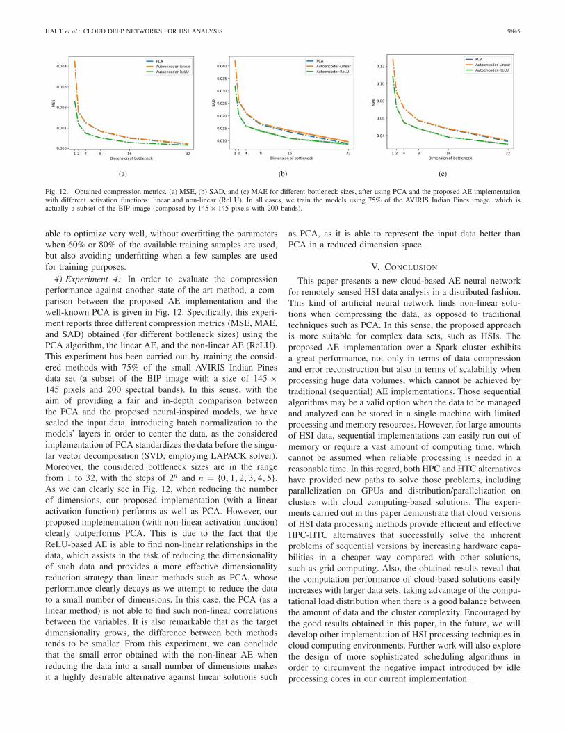
Fig. 12. Obtained compression metrics. (a) MSE, (b) SAD, and (c) MAE for different bottleneck sizes, after using PCA and the proposed AE implementationwith different activation functions: linear and non-linear (ReLU). In all cases, we train the models using 75% of the AVIRIS Indian Pines image, which isactually a subset of the BIP image (composed by 145× 145 pixels with 200 bands).

able to optimize very well, without overfitting the parameterswhen 60% or 80% of the available training samples are used,but also avoiding underfitting when a few samples are usedfor training purposes.

4) Experiment 4: In order to evaluate the compressionperformance against another state-of-the-art method, a com-parison between the proposed AE implementation and thewell-known PCA is given in Fig. 12. Specifically, this experi-ment reports three different compression metrics (MSE, MAE,and SAD) obtained (for different bottleneck sizes) using thePCA algorithm, the linear AE, and the non-linear AE (ReLU).This experiment has been carried out by training the consid-ered methods with 75% of the small AVIRIS Indian Pinesdata set (a subset of the BIP image with a size of 145 ×145 pixels and 200 spectral bands). In this sense, with theaim of providing a fair and in-depth comparison betweenthe PCA and the proposed neural-inspired models, we havescaled the input data, introducing batch normalization to themodels’ layers in order to center the data, as the consideredimplementation of PCA standardizes the data before the singu-lar vector decomposition (SVD; employing LAPACK solver).Moreover, the considered bottleneck sizes are in the rangefrom 1 to 32, with the steps of 2n and n = {0, 1, 2, 3, 4, 5}.As we can clearly see in Fig. 12, when reducing the numberof dimensions, our proposed implementation (with a linearactivation function) performs as well as PCA. However, ourproposed implementation (with non-linear activation function)clearly outperforms PCA. This is due to the fact that theReLU-based AE is able to find non-linear relationships in thedata, which assists in the task of reducing the dimensionalityof such data and provides a more effective dimensionalityreduction strategy than linear methods such as PCA, whoseperformance clearly decays as we attempt to reduce the datato a small number of dimensions. In this case, the PCA (as alinear method) is not able to find such non-linear correlationsbetween the variables. It is also remarkable that as the targetdimensionality grows, the difference between both methodstends to be smaller. From this experiment, we can concludethat the small error obtained with the non-linear AE whenreducing the data into a small number of dimensions makesit a highly desirable alternative against linear solutions such

as PCA, as it is able to represent the input data better thanPCA in a reduced dimension space.

V. CONCLUSION

This paper presents a new cloud-based AE neural networkfor remotely sensed HSI data analysis in a distributed fashion.This kind of artificial neural network finds non-linear solu-tions when compressing the data, as opposed to traditionaltechniques such as PCA. In this sense, the proposed approachis more suitable for complex data sets, such as HSIs. Theproposed AE implementation over a Spark cluster exhibitsa great performance, not only in terms of data compressionand error reconstruction but also in terms of scalability whenprocessing huge data volumes, which cannot be achieved bytraditional (sequential) AE implementations. Those sequentialalgorithms may be a valid option when the data to be managedand analyzed can be stored in a single machine with limitedprocessing and memory resources. However, for large amountsof HSI data, sequential implementations can easily run out ofmemory or require a vast amount of computing time, whichcannot be assumed when reliable processing is needed in areasonable time. In this regard, both HPC and HTC alternativeshave provided new paths to solve those problems, includingparallelization on GPUs and distribution/parallelization onclusters with cloud computing-based solutions. The experi-ments carried out in this paper demonstrate that cloud versionsof HSI data processing methods provide efficient and effectiveHPC-HTC alternatives that successfully solve the inherentproblems of sequential versions by increasing hardware capa-bilities in a cheaper way compared with other solutions,such as grid computing. Also, the obtained results reveal thatthe computation performance of cloud-based solutions easilyincreases with larger data sets, taking advantage of the compu-tational load distribution when there is a good balance betweenthe amount of data and the cluster complexity. Encouraged bythe good results obtained in this paper, in the future, we willdevelop other implementation of HSI processing techniques incloud computing environments. Further work will also explorethe design of more sophisticated scheduling algorithms inorder to circumvent the negative impact introduced by idleprocessing cores in our current implementation.

9846 IEEE TRANSACTIONS ON GEOSCIENCE AND REMOTE SENSING, VOL. 57, NO. 12, DECEMBER 2019

ACKNOWLEDGMENT

The authors would like to thank D. Simmel for his assistancewith the cloud environment, which was made possible throughthe XSEDE Extended Collaborative Support Service (ECSS)Program [65], [66]. They would also like to thank the editorsand the anonymous reviewers for their outstanding commentsand suggestions, which greatly helped to improve the technicalquality and presentation of this paper.

REFERENCES

[1] W. Emery and A. Camps, Basic Electromagnetic Concepts and Applica-tions to Optical Sensors. Amsterdam, The Netherlands: Elsevier, 2017,pp. 43–85.

[2] A. F. H. Goetz, G. Vane, J. E. Solomon, and B. N. Rock, “Imagingspectrometry for earth remote sensing,” Science, vol. 228, no. 4704,pp. 1147–1153, 1985.

[3] M. Teke, H. S. Deveci, O. Haliloglu, S. Zübeyde Gürbüz, andU. Sakarya, “A short survey of hyperspectral remote sensing applicationsin agriculture,” in Proc. 6th Int. Conf. Recent Adv. Space Technol.(RAST), Jun. 2013, pp. 171–176.

[4] A. Plaza, J. Plaza, A. Paz, and S. Sanchez, “Parallel hyperspectral imageand signal processing [applications corner],” IEEE Signal Process. Mag.,vol. 28, no. 3, pp. 119–126, May 2011.

[5] R. O. Green et al., “Imaging spectroscopy and the airborne visi-ble/infrared imaging spectrometer (AVIRIS),” Remote Sens. Environ.,vol. 65, no. 3, pp. 227–248, Sep. 1998.

[6] K. I. Iteen and et al., “APEX - the hyperspectral ESA airborne prismexperiment,” Sensors, vol. 8, no. 10, pp. 6235–6259, 2008.

[7] C. D. A. K. Stephen Babey, “Compact airborne spectrographic imager(CASI): A progress review,” Proc. SPIE, vol. 1937, Jul. 1993,Art. no. 193712. doi: 10.1117/12.157052.

[8] S. G. Ungar, J. S. Pearlman, J. A. Mendenhall, and D. Reuter, “Overviewof the earth observing one (EO-1) mission,” IEEE Trans. Geosci. RemoteSens., vol. 41, no. 6, pp. 1149–1159, Jun. 2003.

[9] M. J. Barnsley, J. J. Settle, M. A. Cutter, D. R. Lobb, and F. Teston,“The PROBA/CHRIS mission: A low-cost smallsat for hyperspec-tral multiangle observations of the Earth surface and atmosphere,”IEEE Trans. Geosci. Remote Sens., vol. 42, no. 7, pp. 1512–1520,Jul. 2004.

[10] L. Guanter and et al., “The EnMAP spaceborne imaging spectroscopymission for earth observation,” Senser, vol. 7, no. 7, pp. 8830–8857,Jul. 2015.

[11] C. Galeazzi, A. Sacchetti, A. Cisbani, and G. Babini, “The PRISMAprogram,” in Proc. IEEE Int. Geosci. Remote Sens. Symp., vol. 4,Jul. 2008, pp. IV-105–IV-108.

[12] M. A. Wulder, J. G. Masek, W. B. Cohen, T. R. Loveland, andC. E. Woodcock, “Opening the archive: How free data has enabled thescience and monitoring promise of Landsat,” Remote Sens. Environ.,vol. 122, pp. 2–10, Jul. 2012.

[13] J. Aschbacher, ESA’s Earth Observation Strategy Copernicus. New York,NY, USA: Singapore, 2017, pp. 81–86. doi: 10.1007/978-981-10-3713-9_5.

[14] Y. Ma et al., “Remote sensing big data computing: Challenges andopportunities,” Future Generat. Comput. Syst., vol. 51, pp. 47–60,Oct. 2015.

[15] M. Chi, A. Plaza, J. A. Benediktsson, Z. Sun, J. Shen, and Y. Zhu, “Bigdata for remote sensing: Challenges and opportunities,” Proc. IEEE,vol. 104, no. 11, pp. 2207–2219, Nov. 2016.

[16] A. Plaza, D. Valencia, J. Plaza, and P. Martinez, “Commodity cluster-based parallel processing of hyperspectral imagery,” J. Parallel Distrib.Comput., vol. 66, pp. 345–358, Mar. 2006.

[17] D. Gorgan, V. Bacu, T. Stefanut, D. Rodila, and D. Mihon, “Grid basedsatellite image processing platform for earth observation applicationdevelopment,” in Proc. IEEE Int. Workshop Intell. Data Acquisition Adv.Comput. Syst. Technol. Appl., Sep. 2009, pp. 247–252.

[18] I. Foster, Y. Zhao, I. Raicu, and S. Lu, “Cloud computing and gridcomputing 360-degree compared,” in Proc. Grid Comput. Environ. Work.(GCE), Nov. 2008, pp. 1–10.

[19] Z. Chen, N. Chen, C. Yang, and L. Di, “Cloud computing enabled Webprocessing service for earth observation data processing,” IEEE J. Sel.Topics Appl. Earth Observat. Remote Sens., vol. 5, no. 6, pp. 1637–1649,Dec. 2012.

[20] A. Plaza, J. Plaza, and D. Valencia, “Impact of platform heterogeneity onthe design of parallel algorithms for morphological processing of high-dimensional image data,” J. Supercomput., vol. 40, no. 1, pp. 81–107,Apr. 2007.

[21] A. Plaza et al., “Recent advances in techniques for hyperspectral imageprocessing,” Remote Sens. Environ., vol. 113, no. 1, pp. S110–S122,Sep. 2009.

[22] G. Hager and G. Wellein, Introduction to High Performens Computingfor Scientists Engineers. Boca Raton, FL, USA: CRC Press, 2010.

[23] K. Stanoevska-Slabeva, T. Wozniak, and S. Ristol, Grid and CloudComputing: A Business Perspective on Technology and Applications.New York, NY, USA: Springer, 2010.

[24] A. Fernández, S. del Río, V. López, A. Bawakid, M. J. del Jesus,J. M. Benítez, and F. Herrera, “Big data with cloud computing:An insight on the computing environment, MapReduce, and program-ming frameworks,” Wiley Interdiscipl. Rev. Data Mining Knowl. Discov-ery, vol. 4, no. 5, pp. 380–409, 2014.

[25] A. W. Services, “Overview of Amazon Web services,” Amazon WebServices, vol. 1, pp. 1–22, Jan. 2017.

[26] Microsoft Azure Cloud Computing Platform; Services, Microsoft,Redmond, WA, USA, 2017.

[27] C. Severance, Using Google App Engine: Start Building Running WebApps Google’s Infrastructure. Newton, MA, USA: O’Reilly, 2009.

[28] J. Dean and S. Ghemawat, “MapReduce: Simplified data processing onlarge clusters,” in Proc. 6th Symp. Operating Syst. Design Implement.(OSDI), San Francisco, CA, USA, 2004, pp. 137–150.

[29] D. Borthakur, “The Hadoop distributed file system: Architecture anddesign,” Hadoop Project Website, vol. 11, no. 2007, p. 21, 2007.

[30] M. Zaharia et al., “Apache spark: A unified engine for big dataprocessing,” Commun. ACM, vol. 59, no. 11, pp. 56–65, 2016.

[31] J. Haut, M. Paoletti, J. Plaza, and A. Plaza, “Cloud implementation of theK-means algorithm for hyperspectral image analysis,” J. Supercomput.,vol. 73, no. 1, pp. 514–529, 2017.

[32] V. A. A. Quirita et al., “A new cloud computing architecture for theclassification of remote sensing data,” IEEE J. Sel. Topics Appl. EarthObserv. Remote Sens., vol. 10, no. 2, pp. 409–416, Feb. 2017.

[33] Y. Zhang et al., “A distributed parallel algorithm based on low-rank andsparse representation for anomaly detection in hyperspectral images,”Sensors, vol. 18, no. 11, p. 3627, Oct. 2018.

[34] J. Setoain, M. Prieto, C. Tenllado, and F. Tirado, “GPU for parallelon-board hyperspectral image processing,” Int. J. High Perform. Comput.Appl., vol. 22, no. 4, pp. 424–437, 2008.

[35] A. J. Plaza and C. I. Chang, High Performance Computing in RemoteSensing. Boca Raton, FL, USA: CRC Press, 2008.

[36] C. González, S. Sánchez, A. Paz, J. Resano, D. Mozos, and A. Plaza,“Use of FPGA or GPU-based architectures for remotely sensed hyper-spectral image processing,” Integration, vol. 46, no. 2, pp. 89–103,Mar. 2013.

[37] J. E. Ball, D. T. Anderson, and C. S. Chan, “Comprehensive surveyof deep learning in remote sensing: Theories, tools, and challengesfor the community,” J. Appl. Remote Sens., vol. 11, no. 4, p. 042609,2017.

[38] S. Kuching, “The performance of maximum likelihood, spectral anglemapper, neural network and decision tree classifiers in hyperspec-tral image analysis,” J. Comput. Sci., vol. 3, no. 6, pp. 419–423,Jul. 2007.

[39] A. Plaza, P. Martínez, J. Plaza, and R. Pérez, “Dimensionality reduc-tion and classification of hyperspectral image data using sequencesof extended morphological transformations,” in IEEE Trans. Geosci.Remote Sens., vol. 43, no. 3, pp. 466–479, Mar. 2005.

[40] D. Tuia, S. Lopez, M. Schaepman, and J. Chanussot, “Foreword to thespecial issue on hyperspectral image and signal processing,” IEEE J. Sel.Topics Appl. Earth Observat. Remote Sens., vol. 5, no. 2, pp. 347–353,Apr. 2015.

[41] Z. Wu, Y. Li, A. Plaza, J. Li, F. Xiao, and Z. Wei, “Parallel anddistributed dimensionality reduction of hyperspectral data on cloudcomputing architectures,” IEEE J. Sel. Topics Appl. Earth Observ.Remote Sens., vol. 9, no. 6, pp. 2270–2278, Jun. 2016.

[42] F. Del Frate, G. Licciardi, and R. Duca, “Autoassociative neural networksfor features reduction of hyperspectral data,” in Proc. 1st WorkshopHyperspectral Image Signal Process. Evol. Remote Sens., Aug. 2009,pp. 1–4.

[43] G. A. Licciardi and F. D. Frate, “Pixel unmixing in hyperspectral data bymeans of neural networks,” IEEE Trans. Geosci. Remote Sens., vol. 49,no. 11, pp. 4163–4172, Nov. 2011.

HAUT et al.: CLOUD DEEP NETWORKS FOR HSI ANALYSIS 9847

[44] X. Jia, B.-K. Kuo, and M. M. Crawford, “Feature mining for hyper-spectral image classification,” Proc. IEEE, vol. 101, no. 3, pp. 676–697,Mar. 2013.

[45] R. Bellman, Adaptive Control Processes: A Guided Tour. Princeton,NJ, USA: Princeton Univ. Press, 2015.

[46] G. Hughes, “On the mean accuracy of statistical pattern recognizers,”IEEE Trans. Inf. Theory, vol. 14, no. 1, pp. 55–63, Jan. 1968.

[47] X. Kang, P. Duan, S. Li, and J. A. Benediktsson, “Decolorization-basedhyperspectral image visualization,” IEEE Trans. Geosci. Remote Sens.,vol. 56, no. 8, pp. 4346–4360, Aug. 2018.

[48] X. Kang, P. Duan, X. Xiang, S. Li, and J. A. Benediktsson, “Detectionand correction of mislabeled training samples for hyperspectral imageclassification,” IEEE Trans. Geosci. Remote Sens., vol. 56, no. 10,pp. 5673–5686, Oct. 2018.

[49] X. Kang, X. Zhang, S. Li, K. Li, J. Li, and J. A. Benediktsson,“Hyperspectral anomaly detection with attribute and edge-preservingfilters,” IEEE Trans. Geosci. Remote Sens., vol. 55, no. 10,pp. 5600–5611, Oct. 2017.

[50] T.-W. Lee, “Independent component analysis,” in Independent Compo-nent Analysis. New York, NY, USA: Springer, 1998, pp. 27–66.

[51] J. Wang and C.-I. Chang, “Independent component analysis-baseddimensionality reduction with applications in hyperspectral image analy-sis,” IEEE Trans. Geosci. Remote Sens., vol. 44, no. 6, pp. 1586–1600,Jun. 2006.

[52] A. A. Green, M. Berman, P. Switzer, and M. D. Craig, “A transformationfor ordering multispectral data in terms of image quality with implica-tions for noise removal,” IEEE Trans. Geosci. Remote Sens., vol. 26,no. 1, pp. 65–74, Jan. 1988.

[53] N. He et al., “Feature extraction with multiscale covariance maps forhyperspectral image classification,” IEEE Trans. Geosci. Remote Sens.,vol. 57, no. 2, pp. 755–769, Feb. 2018.

[54] S. Wold, K. Esbensen, and P. Geladi, “Principal component analy-sis,” Chemometrics Intell. Lab. Syst., vol. 2, nos. 1–3, pp. 37–52,1987.

[55] D. Fernandez, C. Gonzalez, D. Mozos, and S. Lopez, “FPGA implemen-tation of the principal component analysis algorithm for dimensionalityreduction of hyperspectral images,” J. Real-Time Image Process., vol. 1,pp. 1–12, Nov. 2016.

[56] E. Martel et al., “Implementation of the principal component analysisonto high-performance computer facilities for hyperspectral dimension-ality reduction: Results and comparisons,” Remote Sens., vol. 10, no. 6,p. 864, 2018.

[57] Y. Chen, Z. Lin, X. Zhao, G. Wang, and Y. Gu, “Deep learning-basedclassification of hyperspectral data,” IEEE J. Sel. Topics Appl. EarthObserv. Remote Sens., vol. 7, no. 6, pp. 2094–2107, Jun. 2014.

[58] V. Nair and G. E. Hinton, “Rectified linear units improve restrictedboltzmann machines,” in Proc. 27th Int. Conf. Mach. Learn., 2010,pp. 807–814.

[59] G. E. Hinton and R. S. Zemel, “Autoencoders, minimum descrip-tion length and Helmholtz free energy,” in Proc. 6th Int. Conf.Neural Inf. Process. Syst., 1993, pp. 3–10. [Online]. Available:http://dl.acm.org/citation.cfm?id=2987189.2987190

[60] M. S. Apostolopoulou, D. G. Sotiropoulos, I. E. Livieris, and P. Pintelas,“A memoryless BFGS neural network training algorithm,” in Proc. 7thIEEE Int. Conf. Ind. Inform., Jun. 2009, pp. 216–221.

[61] N. M. Nawi, M. R. Ransing, and R. S. Ransing, “An improved learn-ing algorithm based on the Broyden-fletcher-goldfarb-shanno (BFGS)method for back propagation neural networks,” in Proc. 6th Int. Conf.Intell. Syst. Design Appl., vol. 1, Oct. 2006, pp. 152–157.

[62] R. Fletcher and M. J. D. Powell, “A rapidly convergent descentmethod for minimization,” Comput. J., vol. 6, no. 2, pp. 163–168,Aug. 1963.

[63] Q. V. Le, J. Ngiam, A. Coates, A. Lahiri, B. Prochnow, and A. Y. Ng,“On optimization methods for deep learning,” in Proc. 28th Int. Conf.Int. Conf. Mach. Learn., 2011, pp. 265–272.

[64] N. Wilkins-Diehr et al., “An overview of the XSEDE extended collabo-rative support program,” in Proc. Int. Conf. Supercomput. Mex., vol. 595,May 2016, pp. 3–13.

[65] J. Towns et al., “XSEDE: Accelerating scientific discovery,” Comput.Sci. Eng., vol. 16, no. 5, pp. 62–74, Sep./Oct. 2014.

[66] D. S. G. Cavallaro, and J. M. Haut, “XSEDE project TG-asc180012:Cloud-based distributed autoencoder for hyperspectral images compres-sion,” XSEDE, Tech. Rep., 2019.

[67] J. Pearlman, S. Carman, C. Segal, P. Jarecke, P. Clancy, and W. Browne,“Overview of the hyperion imaging spectrometer for the NASA EO-1mission,” in Proc. IGARSS, vol. 7, Jul. 2001, pp. 3036–3038 vol.7.

Juan Mario Haut (S’17) received the B.Sc. andM.Sc. degrees in computer engineering from theUniversity of Extremadura, Cáceres, Spain, in 2011and 2014, respectively, and the Ph.D. degree ininformation technology from the University ofExtremadura through a University Teacher TrainingProgramme from the Spanish Ministry of Educationin 2019.

He is currently a member of the HyperspectralComputing Laboratory, Department of Computerand Communication, University of Extremadura. His

research interests include remote sensing and the analysis of very high-spectral resolution with the current focus on machine (deep) learning andcloud computing.

Dr. Haut was a recipient of the recognition of Best Reviewers of theIEEE GEOSCIENCE AND REMOTE SENSING LETTERS in 2019. He hasbeen a manuscript reviewer of IEEE TRANSACTIONS ON GEOSCIENCE ANDREMOTE SENSING, the IEEE JOURNAL OF SELECTED TOPICS IN APPLIED

EARTH OBSERVATIONS AND REMOTE SENSING, and IEEE GEOSCIENCE

AND REMOTE SENSING LETTERS.

Jose Antonio Gallardo received the B.Sc. degreein computer engineering from the University ofExtremadura, Cáceres, Spain, in 2019, where hehas been developing his final degree work at theHyperspectral Computing Laboratory, Departmentof Computers and Communications.

Mercedes E. Paoletti (S’17) received the B.Sc.and M.Sc. degrees in computer engineering fromthe University of Extremadura, Cáceres, Spain,in 2014 and 2016, respectively, where she is cur-rently pursuing the Ph.D. degree through a Univer-sity Teacher Training Programme from the SpanishMinistry of Education.

She is currently a member of the HyperspectralComputing Laboratory, Department of Technologyof Computers and Communications, University ofExtremadura. Her research interests include remote

sensing and analysis of very high spectral resolution with the current focuson deep learning and high-performance computing.

Gabriele Cavallaro (S’13–M’17) received the B.S.and M.S. degrees in telecommunications engi-neering from the University of Trento, Trento,Italy, in 2011 and 2013, respectively, and thePh.D. degree in electrical and computer engineeringfrom the University of Iceland, Reykjavík, Iceland,in 2016.

He is currently a Post-Doctoral Research Assistantwith the Juelich Supercomputing Centre, Jülich,Germany, where he is also a part of a scientificresearch group focused on high-productivity data

processing within the Federated Systems and Data Division. His researchinterests include remote sensing image processing with parallel machinelearning algorithms that scale on high performance and distributed systems.

Dr. Cavallaro was a recipient of the IEEE GRSS Third Prize in the StudentPaper Competition of the 2015 IEEE International Geoscience and RemoteSensing Symposium, Milan, Italy, in July 2015.

9848 IEEE TRANSACTIONS ON GEOSCIENCE AND REMOTE SENSING, VOL. 57, NO. 12, DECEMBER 2019

Javier Plaza (M’09–SM’15) received the M.Sc.and Ph.D. degrees in computer engineering fromthe Hyperspectral Computing Laboratory, Depart-ment of Technology of Computers and Communi-cations, University of Extremadura, Cáceres, Spain,in 2004 and 2008, respectively.

He is currently a member of the HyperspectralComputing Laboratory, Department of Technologyof Computers and Communications, University ofExtremadura. He has authored more than 150 pub-lications, including over 50 JCR journal papers, ten

book chapters, and 90 peer-reviewed conference proceeding papers. His mainresearch interests include hyperspectral data processing and parallel computingof remote sensing data.

Dr. Plaza was a recipient of the Outstanding Ph.D. Dissertation Awardat the University of Extremadura in 2008. He was also a recipient of theBest Column Award of the IEEE Signal Processing Magazine in 2015 andthe Most Highly Cited Paper (2005–2010) in the Journal of Parallel andDistributed Computing. He received the best paper awards at the IEEEInternational Conference on Space Technology and the IEEE Symposiumon Signal Processing and Information Technology. He has guest edited fourspecial issues on hyperspectral remote sensing for different journals. He isalso an Associate Editor of the IEEE GEOSCIENCE AND REMOTE SENSING

LETTERS and IEEE Remote Sensing Code Library. Additional information:http://www.umbc.edu/rssipl/people/jplaza

Antonio Plaza (M’05–SM’07–F’15) received theM.Sc. degree and the Ph.D. degree in computerengineering from the Hyperspectral Computing Lab-oratory, the Department of Technology of Computersand Communications, University of Extremadura,Cáceres, Spain, in 1999 and 2002, respectively.

He is currently the Head of the HyperspectralComputing Laboratory, Department of Technologyof Computers and Communications, University ofExtremadura. He has authored more than 600 publi-cations, including over 200 JCR journal papers (over

160 in IEEE journals), 23 book chapters, and around 300 peer-reviewedconference proceeding papers. His research interests include hyperspectraldata processing and parallel computing of remote sensing data.

Dr. Plaza was a member of the Editorial Board of the IEEE Geoscience andRemote Sensing Newsletter from 2011 to 2012 and the IEEE GEOSCIENCEAND REMOTE SENSING MAGAZINE in 2013. He was also a member ofthe Steering Committee of the IEEE JOURNAL OF SELECTED TOPICS IN

APPLIED EARTH OBSERVATIONS AND REMOTE SENSING (JSTARS). He is

also a fellow of IEEE for contributions to hyperspectral data processingand parallel computing of earth observation data. He was a recipient ofthe recognition of Best Reviewers of the IEEE GEOSCIENCE AND REMOTESENSING LETTERS in 2009 and the Best Reviewer of the IEEE TRANSAC-TIONS ON GEOSCIENCE AND REMOTE SENSING in 2010, for which he hasserved as an Associate Editor from 2007 to 2012. He was also a recipient ofthe Best Column Award of the IEEE Signal Processing Magazine in 2015,the 2013 Best Paper Award of the JSTARS journal, and the Most Highly CitedPaper (2005–2010) in the Journal of Parallel and Distributed Computing.He received best paper awards at the IEEE International Conference on SpaceTechnology and the IEEE Symposium on Signal Processing and InformationTechnology. He has served as the Director of Education Activities for the IEEEGeoscience and Remote Sensing Society (GRSS) from 2011 to 2012 and as thePresident of the Spanish Chapter of IEEE GRSS from 2012 to 2016. He hasreviewed more than 500 manuscripts for over 50 different journals. He hasserved as the Editor-in-Chief of the IEEE TRANSACTIONS ON GEOSCIENCE

AND REMOTE SENSING from 2013 to 2017. He has guest edited ten specialissues on hyperspectral remote sensing for different journals. He is alsoan Associate Editor of the IEEE ACCESS (receiving the recognition as anOutstanding Associate Editor of the journal in 2017). Additional information:http://www.umbc.edu/rssipl/people/aplaza

Morris Riedel (M’10) received the Ph.D. degreefrom the Karlsruhe Institute of Technology (KIT),Karlsruhe, Germany.

He started the work in parallel and distributedsystems in the field of scientific visualization andcomputational steering of e-Science applications onlarge-scale HPC resources. He held various posi-tions at the Jülich Supercomputing Centre, Jülich,Germany. At this institute, he is also the Headof a specific scientific research group focused onhigh productivity data processing as a part of the

Federated Systems and Data Division. He is currently an Adjunct AssociateProfessor with the Department of Mechanical Engineering and ComputerScience, University of Iceland, Reykjavík, Iceland.