cloud lc04 warehouse-scale...

(C) 2013 Marcel Graf

HES-SO | Master of Science in Engineering

Cloud Computing — Warehouse-Scale Computing

Academic year 2013/2014

HES-SO | MSE

Cloud Computing | Warehouse-Scale Computing | Academic year 2013/2014 (C) 2013 Marcel Graf

Warehouse-scale computersIntroduction

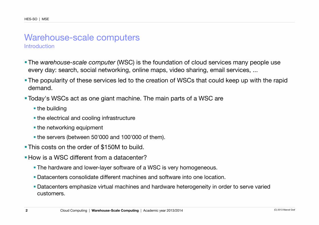
■The warehouse-scale computer (WSC) is the foundation of cloud services many people use every day: search, social networking, online maps, video sharing, email services, ...■The popularity of these services led to the creation of WSCs that could keep up with the rapid

demand.■Today's WSCs act as one giant machine. The main parts of a WSC are

■ the building■ the electrical and cooling infrastructure■ the networking equipment■ the servers (between 50'000 and 100'000 of them).

■This costs on the order of $150M to build.■How is a WSC different from a datacenter?

■ The hardware and lower-layer software of a WSC is very homogeneous.■ Datacenters consolidate different machines and software into one location.■ Datacenters emphasize virtual machines and hardware heterogeneity in order to serve varied

customers.

2

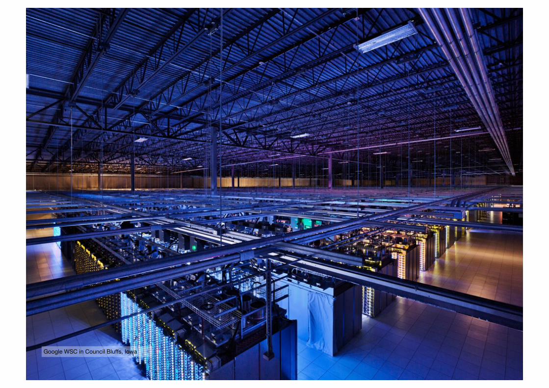
Google WSC in Council Bluffs, Iowa

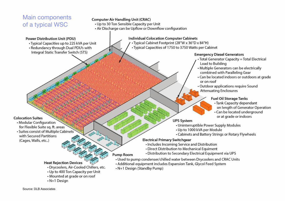
Source: DLB Associates

Main componentsof a typical WSC

HES-SO | MSE


Warehouse-scale computersMain components

5

HES-SO | MSE


Warehouse-scale computersGoals and requirements for a WSC architect

6

■ Important design factors for a WSC:■ Optimize cost-performance

■ Small savings add up. A 10% reduction in cost can save $15M.

■ Increase energy-efficiency■ If servers are not energy-efficient they increase (1)

cost of electricity, (2) cost of infrastructure to provide electricity, (3) cost of infrastructure to cool the servers.

■ Optimize computation per joule

■ Dependability via redundancy■ Hardware and software in a WSC must

collectively provide at least 99.99% availability while individual servers are much less reliable.

■ → Redundant servers and smart software

■ Sufficient network I/O bandwidth■ Networking is needed to interface to the public,

but also to keep data consistent between multiple WSCs.

■ Both interactive and batch-processing workloads■ Search and social networks require fast response

times.■ Indexing, Big Data analytics etc. create a lot of

batch processing workloads.

■ Ample parallelism■ SaaS workload consists of independent requests

of millions of users: request-level parallelism■ Data of many batch applications can be

processed in independent chunks: data-level parallelism

■ Operational costs count■ Building, electrical and cooling infrastructure

contribute significantly to cost.

■ Opportunities / problems associated with scale■ Big economies of scale because of the massive

size (e.g., purchase customized servers)■ But also high failure rates

HES-SO | MSE


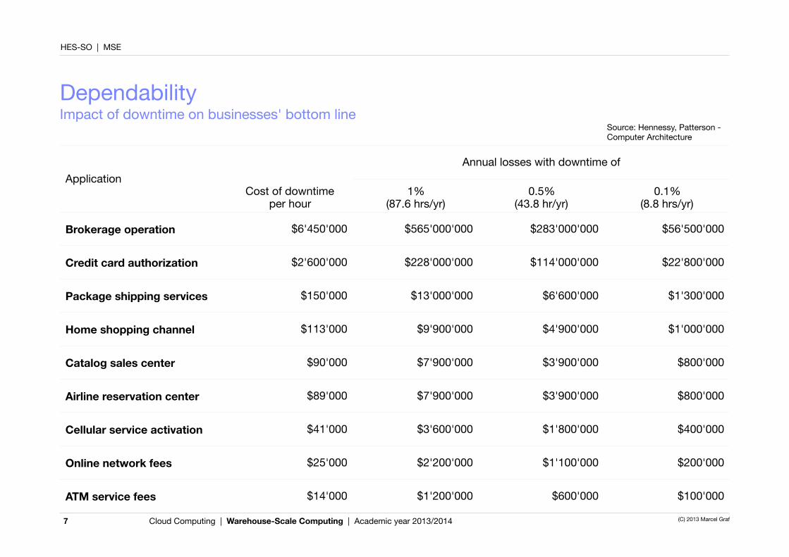
DependabilityImpact of downtime on businesses' bottom line

7

ApplicationAnnual losses with downtime ofAnnual losses with downtime ofAnnual losses with downtime of

ApplicationCost of downtime

per hour1%

(87.6 hrs/yr)0.5%

(43.8 hr/yr)0.1%

(8.8 hrs/yr)

Brokerage operation $6'450'000 $565'000'000 $283'000'000 $56'500'000

Credit card authorization $2'600'000 $228'000'000 $114'000'000 $22'800'000

Package shipping services $150'000 $13'000'000 $6'600'000 $1'300'000

Home shopping channel $113'000 $9'900'000 $4'900'000 $1'000'000

Catalog sales center $90'000 $7'900'000 $3'900'000 $800'000

Airline reservation center $89'000 $7'900'000 $3'900'000 $800'000

Cellular service activation $41'000 $3'600'000 $1'800'000 $400'000

Online network fees $25'000 $2'200'000 $1'100'000 $200'000

ATM service fees $14'000 $1'200'000 $600'000 $100'000

Source: Hennessy, Patterson - Computer Architecture

HES-SO | MSE


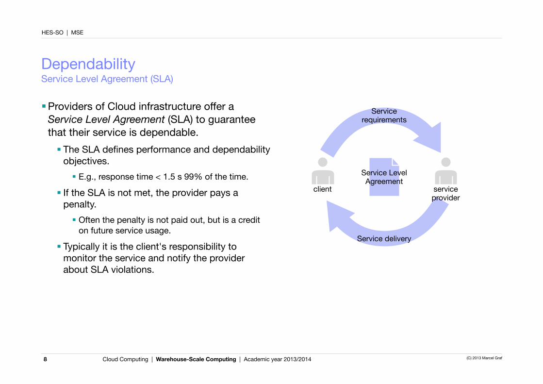
DependabilityService Level Agreement (SLA)

■Providers of Cloud infrastructure offer a Service Level Agreement (SLA) to guarantee that their service is dependable.■ The SLA defines performance and dependability

objectives.■ E.g., response time < 1.5 s 99% of the time.

■ If the SLA is not met, the provider pays a penalty.■ Often the penalty is not paid out, but is a credit

on future service usage.

■ Typically it is the client's responsibility to monitor the service and notify the provider about SLA violations.

8

client serviceprovider

Service LevelAgreement

Service requirements

Service delivery

HES-SO | MSE


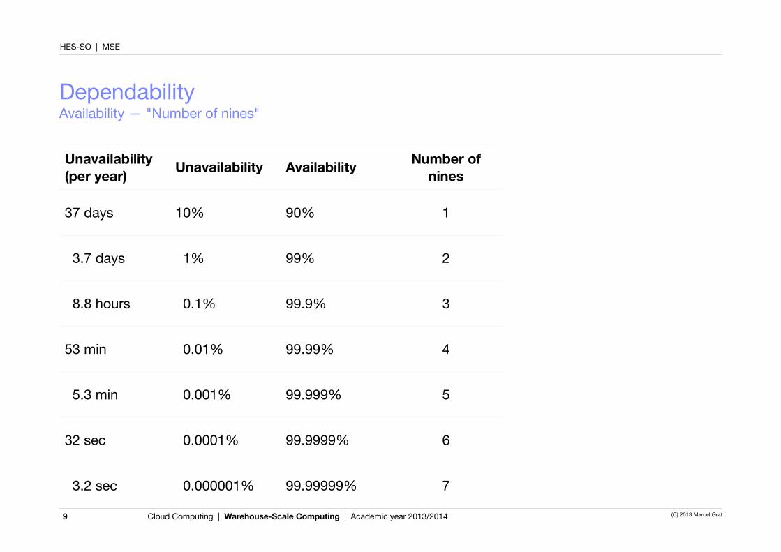
DependabilityAvailability — "Number of nines"

9

Unavailability (per year) Unavailability Availability Number of

nines

37 days 10% 90% 1

3.7 days 1% 99% 2

8.8 hours 0.1% 99.9% 3

53 min 0.01% 99.99% 4

5.3 min 0.001% 99.999% 5

32 sec 0.0001% 99.9999% 6

3.2 sec 0.000001% 99.99999% 7

HES-SO | MSE


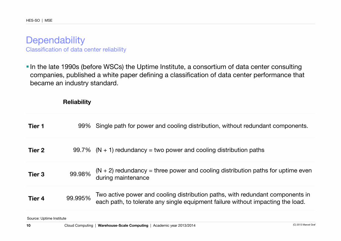
DependabilityClassification of data center reliability

10

Reliability

Tier 1 99% Single path for power and cooling distribution, without redundant components.

Tier 2 99.7% (N + 1) redundancy = two power and cooling distribution paths

Tier 3 99.98% (N + 2) redundancy = three power and cooling distribution paths for uptime even during maintenance

Tier 4 99.995% Two active power and cooling distribution paths, with redundant components in each path, to tolerate any single equipment failure without impacting the load.

Source: Uptime Institute

■ In the late 1990s (before WSCs) the Uptime Institute, a consortium of data center consulting companies, published a white paper defining a classification of data center performance that became an industry standard.

HES-SO | MSE


DependabilitySystems and their components

11

■Computer systems are designed and constructed at different layers of abstraction. The dependability of a system is a function of the dependability of its components (modules).■When zooming in on a

component we see that it is itself a system composed of components, and so on.

■Some faults are widespread, like loss of electricity, while others are limited to a single component.

systemmodulesub-modulesub-sub-module

HES-SO | MSE


DependabilityService Level Agreement (SLA)

12

■Systems alternate between two states of service with respect to an SLA:■ Service accomplishment: The service is

delivered as specified.■ Service interruption: The delivered service is

different from the SLA.■Transition from accomplishment to interruption

is caused by a failure.■A restoration brings the service back into the

accomplishment state.

Service accomplishement

Service interruption

Failure

Restoration

HES-SO | MSE


DependabilityModule reliability metrics

■ Industry dependability metrics often make the following assumptions:■ A module is observed from a reference initial

instant.■When the module fails, it is repaired and

becomes as new.■ The time to failure of a module is a random

variable with exponential distribution, i.e. the probability of failure does not depend on the age.

■ The failures of different modules in a system are independent.

■Module reliability metrics■Mean time to failure (MTTF): Measure of

continuous service accomplishment from a reference initial instant.

■ Failure in time (FIT): Reciprocal of MTTF, reported as failures per 109 hours, i.e. FIT = 109 hours / MTTF

■Mean time to repair (MTTR): Measure of service interruption.

■Mean time between failures (MTBF): MTBF = MTTF + MTTR

■Module availability metrics■Module availability = MTTF / (MTTF + MTTR)

13

failure

MTTF

restoration

MTTR0

failure restoration

MTBF

time

HES-SO | MSE


DependabilityExample: Disk subsystem

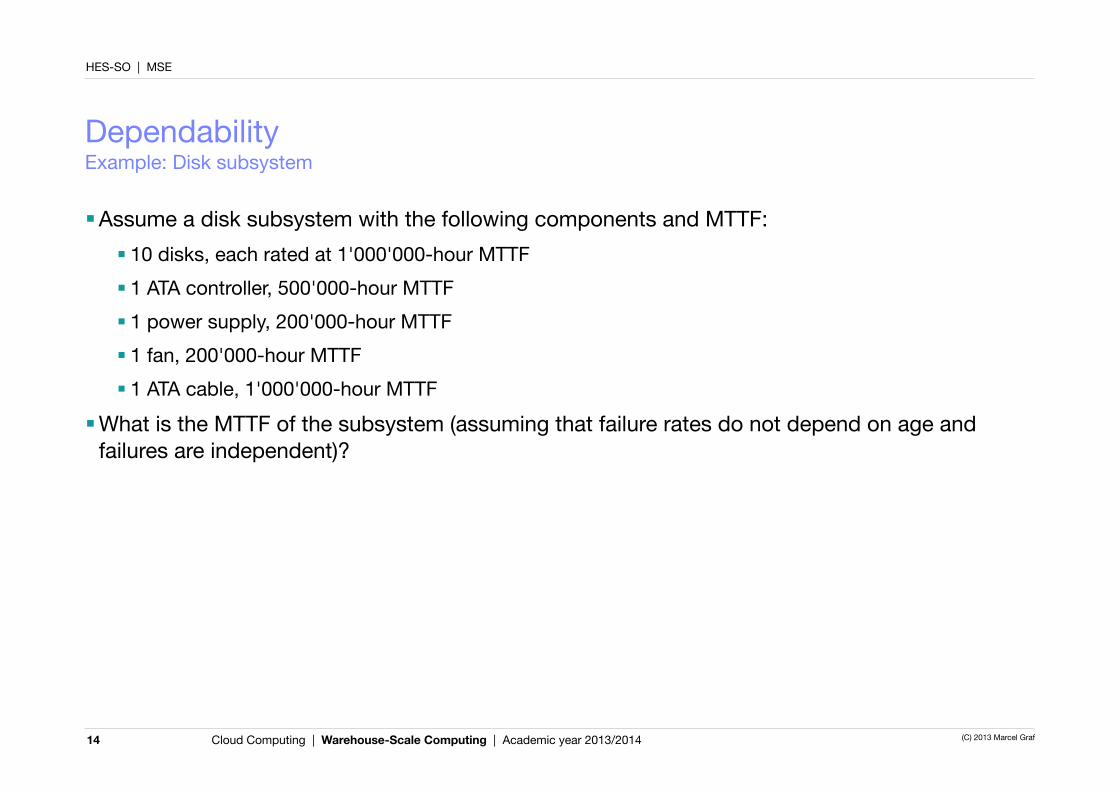
■Assume a disk subsystem with the following components and MTTF:■ 10 disks, each rated at 1'000'000-hour MTTF■ 1 ATA controller, 500'000-hour MTTF■ 1 power supply, 200'000-hour MTTF■ 1 fan, 200'000-hour MTTF■ 1 ATA cable, 1'000'000-hour MTTF

■What is the MTTF of the subsystem (assuming that failure rates do not depend on age and failures are independent)?

14

HES-SO | MSE


DependabilityExample: Disk subsystem

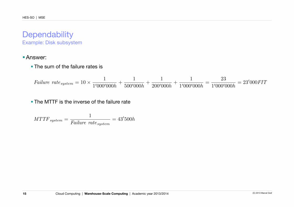
■Answer:■ The sum of the failure rates is

■ The MTTF is the inverse of the failure rate

15

Failure ratesystem = 10⇥ 1

100000000h+

1

5000000h+

1

2000000h+

1

100000000h=

23

100000000h= 230000FIT

MTTF system =1

Failure ratesystem= 430500h

HES-SO | MSE


DependabilityExample: Redundant power supplies

■The power supply of the disk subsystem has only 200'000-hour MTTF. To improve dependability another power supply is added. The disk subsystem can run using a single power supply. What is the dependability of the pair?

16

HES-SO | MSE


DependabilityExample: Redundant power supplies

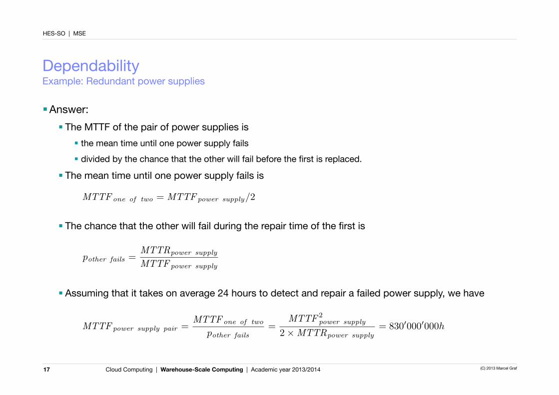
■Answer:■ The MTTF of the pair of power supplies is

■ the mean time until one power supply fails■ divided by the chance that the other will fail before the first is replaced.

■ The mean time until one power supply fails is

■ The chance that the other will fail during the repair time of the first is

■ Assuming that it takes on average 24 hours to detect and repair a failed power supply, we have

17

MTTFone of two

= MTTFpower supply

/2

MTTFpower supply pair

=MTTF

one of two

pother fails

=MTTF 2

power supply

2⇥MTTRpower supply

= 83000000000h

pother fails

=MTTR

power supply

MTTFpower supply

HES-SO | MSE


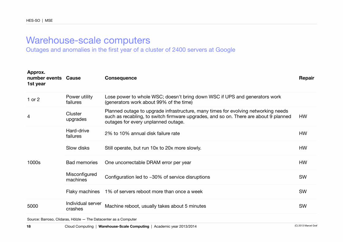
Warehouse-scale computersOutages and anomalies in the first year of a cluster of 2400 servers at Google

18

Approx. number events 1st year

Cause Consequence Repair

1 or 2 Power utility failures

Lose power to whole WSC; doesn't bring down WSC if UPS and generators work (generators work about 99% of the time)

4 Cluster upgrades

Planned outage to upgrade infrastructure, many times for evolving networking needs such as recabling, to switch firmware upgrades, and so on. There are about 9 planned outages for every unplanned outage.

HW

1000s

Hard-drive failures 2% to 10% annual disk failure rate HW

1000s

Slow disks Still operate, but run 10x to 20x more slowly. HW

1000s Bad memories One uncorrectable DRAM error per year HW1000s

Misconfigured machines Configuration led to ~30% of service disruptions SW

1000s

Flaky machines 1% of servers reboot more than once a week SW

5000 Individual server crashes Machine reboot, usually takes about 5 minutes SW

Source: Barroso, Clidaras, Hölzle — The Datacenter as a Computer

HES-SO | MSE


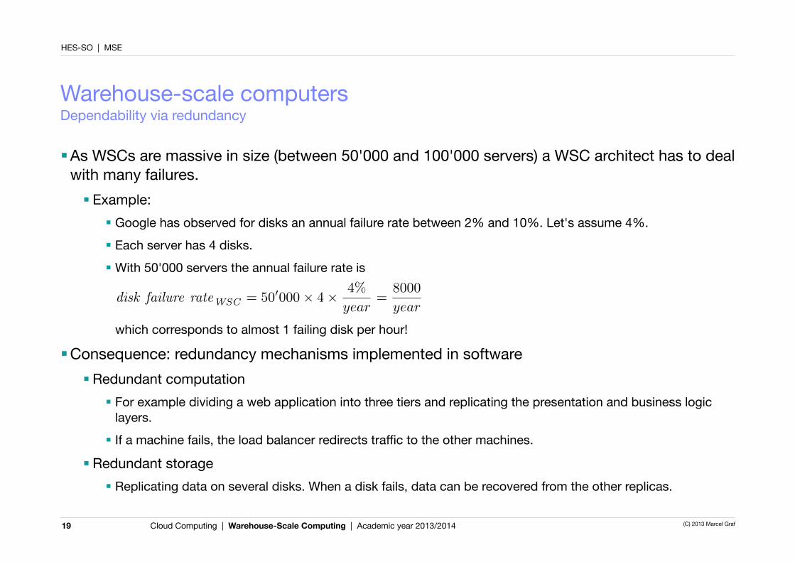
Warehouse-scale computersDependability via redundancy

■As WSCs are massive in size (between 50'000 and 100'000 servers) a WSC architect has to deal with many failures.■ Example:

■ Google has observed for disks an annual failure rate between 2% and 10%. Let's assume 4%. ■ Each server has 4 disks.■ With 50'000 servers the annual failure rate is

which corresponds to almost 1 failing disk per hour!

■Consequence: redundancy mechanisms implemented in software■ Redundant computation

■ For example dividing a web application into three tiers and replicating the presentation and business logic layers.

■ If a machine fails, the load balancer redirects traffic to the other machines.

■ Redundant storage■ Replicating data on several disks. When a disk fails, data can be recovered from the other replicas.

19

disk failure rateWSC = 500000⇥ 4⇥ 4%

year=

8000

year

HES-SO | MSE


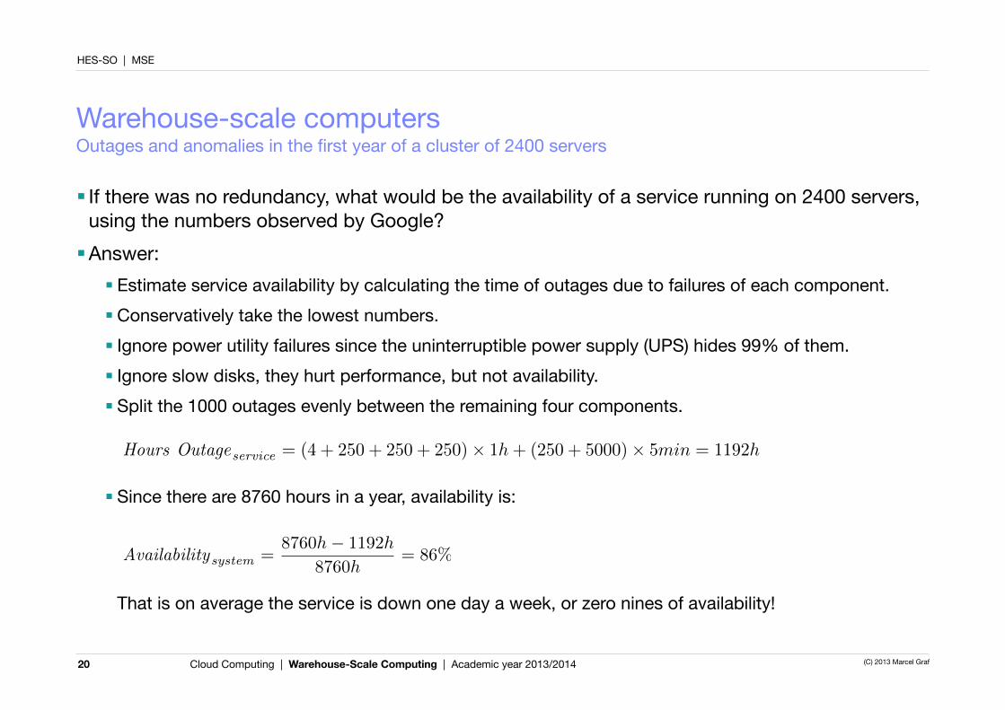
Warehouse-scale computersOutages and anomalies in the first year of a cluster of 2400 servers

20

■ If there was no redundancy, what would be the availability of a service running on 2400 servers, using the numbers observed by Google?■Answer:

■ Estimate service availability by calculating the time of outages due to failures of each component.■Conservatively take the lowest numbers.■ Ignore power utility failures since the uninterruptible power supply (UPS) hides 99% of them.■ Ignore slow disks, they hurt performance, but not availability.■ Split the 1000 outages evenly between the remaining four components.

■ Since there are 8760 hours in a year, availability is:

That is on average the service is down one day a week, or zero nines of availability!

Hours Outageservice = (4 + 250 + 250 + 250)⇥ 1h+ (250 + 5000)⇥ 5min = 1192h

Availabilitysystem =8760h� 1192h

8760h= 86%

HES-SO | MSE


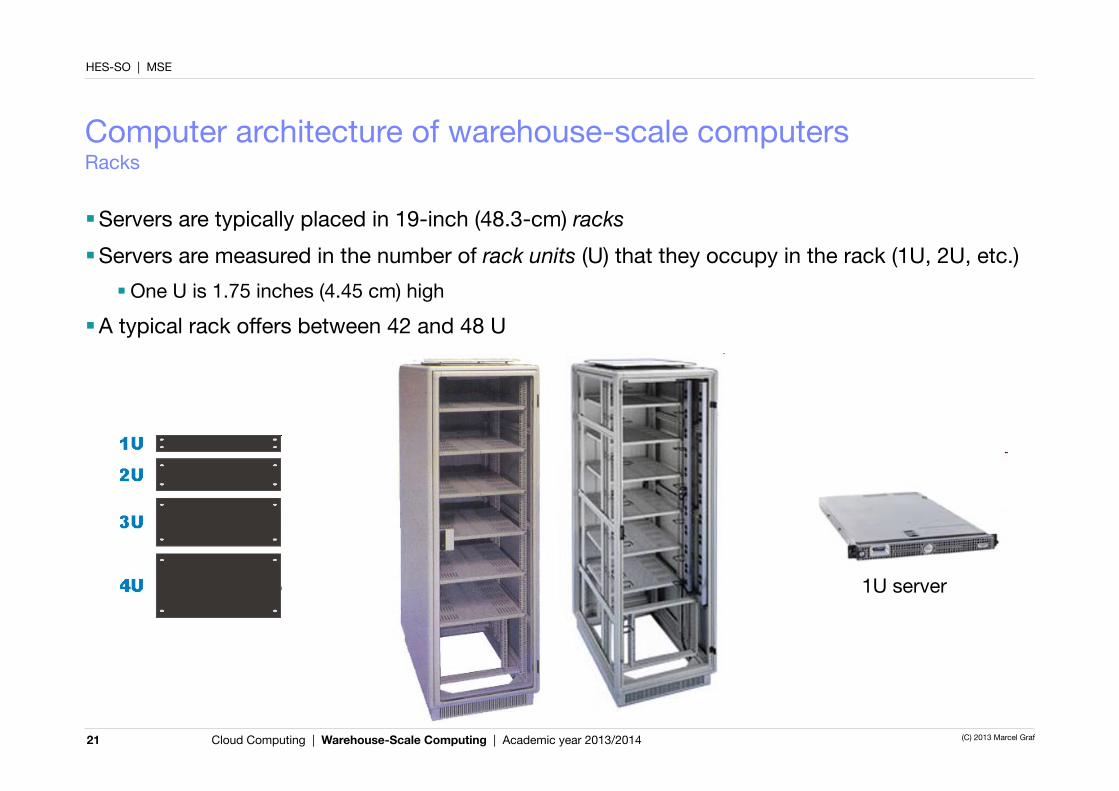
Computer architecture of warehouse-scale computersRacks

■Servers are typically placed in 19-inch (48.3-cm) racks■Servers are measured in the number of rack units (U) that they occupy in the rack (1U, 2U, etc.)

■One U is 1.75 inches (4.45 cm) high■A typical rack offers between 42 and 48 U

21

Racks

� Equipment (e.g., servers) are typically placed in racks

� Equipment are designed in a modular fashion to fit into rack units(1U, 2U etc.)

� A single rack can hold up to 42 1U servers

6

1U Server

7U Blade center

© Carnegie Mellon University in Qatar

1U server

HES-SO | MSE


Computer architecture of warehouse-scale computersNetworking

■WSCs use a hierarchy of networks■ Rack switch

■ Located inside a rack■ Up to 48 ports, one for each server in the rack,

typically 1 Gbit/s Ethernet links■ → Bandwidth is homogeneous within the

rack■ 4 to 8 uplinks to the next higher switch in the

network hierarchy■ Ratio between internal bandwidth and uplink

bandwidth is called oversubscription factor (typically between 10 and 5)

■ Array switch■ Connects an array of 30 racks■ More than ten times more expensive (per port)

than a rack switch■ → Bandwidth between racks is reduced

22

Row of servers in a Google WSC, 2012

HES-SO | MSE


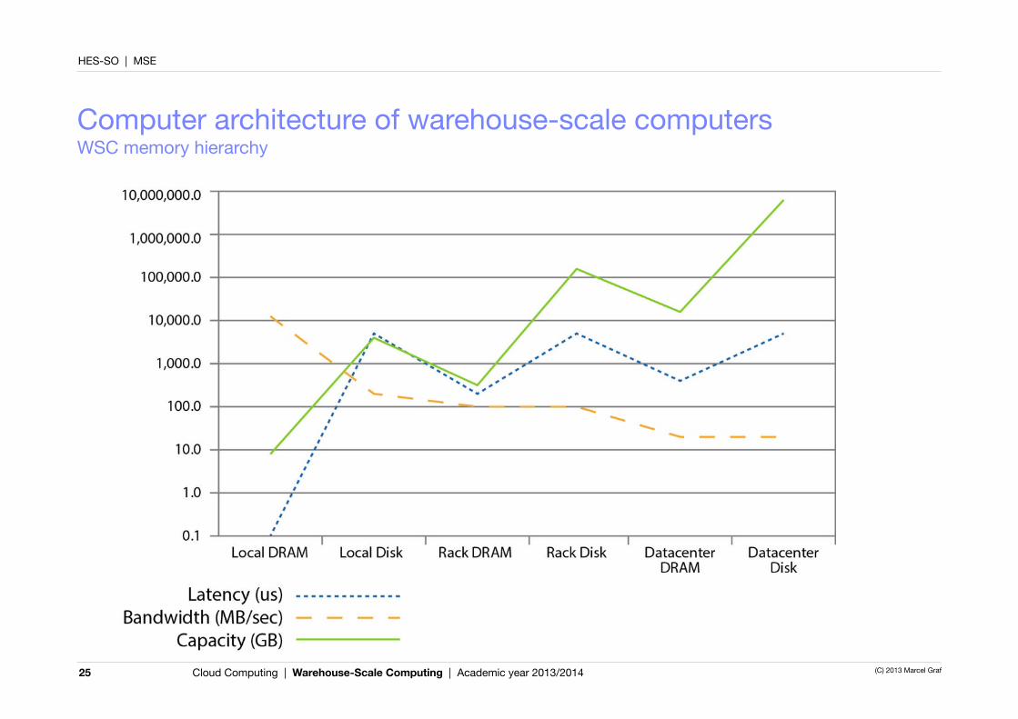
Computer architecture of warehouse-scale computersWSC memory hierarchy

24

■A rack contains 80 servers, thus■ 1 TB memory■ 160 TB disk

■Between two servers in the same rack■memory 300 µs access time

and transfers at 100 MB/sec■ disk 11 ms access time and

transfers at 100 MB/sec

■An array of 30 racks contains 2400 servers, thus■ 30 TB memory■ 4.8 PB disk

■Between two servers in different racks■memory 500 µs access time

and transfers at 10 MB/sec■ disk 12 ms access time and

transfers at 10 MB/sec

■A server contains■ 16 GB memory with 100 ns

access time and transfers at 20 GB/sec

■ a 2 TB disk with 10 ms access time and transfers at 200 MB/sec

■ 2 CPU sockets■ 1 x 1 GBit/s Ethernet port

HES-SO | MSE



25

HES-SO | MSE



■Network overhead dramatically increases latency for DRAM■ but still more than 10 times better than local disk

■Bandwidth differences between DRAM and disk are collapsed by network■Consequence: Management software tries to keep communication local by placing cooperating

tasks first in the same server, second in the same rack or third in the same array.

26

HES-SO | MSE


Computer architecture of warehouse-scale computersExample: Data transfer performance

27

■How long does it take to transfer 1000 MB between disks ■within the server■ between servers in the rack■ between servers in different racks in the array?

■How much faster is it to transfer 1000 MB between DRAM in the three cases?

HES-SO | MSE


Computer architecture of warehouse-scale computersExample: Data transfer performance

■Answer:■ A 1000 MB transfer between disks takes

■ within servers: 5 sec■ within rack: 10 sec■ within array: 100 sec

■ A memory-to-memory block transfer takes■ within server: 0.05 sec■ within rack: 10 sec■ within array: 100 sec

28

HES-SO | MSE


Computer architecture of warehouse-scale computersWSC network hierarchy

29

Rack (80 servers with

rack switch)

Array switch

... ...

Load balancer

Layer 3access router

Internet

Layer 3core router

...

Internet

Datacenterlayer 3

Datacenterlayer 2

Redrawn from: James Hamilton, Amazon, http://mvdirona.com/jrh/TalksAndPapers/JamesHamilton_AmazonOpenHouse20110607.pdf

HES-SO | MSE


Physical infrastructure and costsPower distribution

30

End-to-end efficiency from high-voltage line to server: 89%

HES-SO | MSE


Physical infrastructure and costsCooling

31

HES-SO | MSE


Physical infrastructure and costsMeasuring efficiency

32

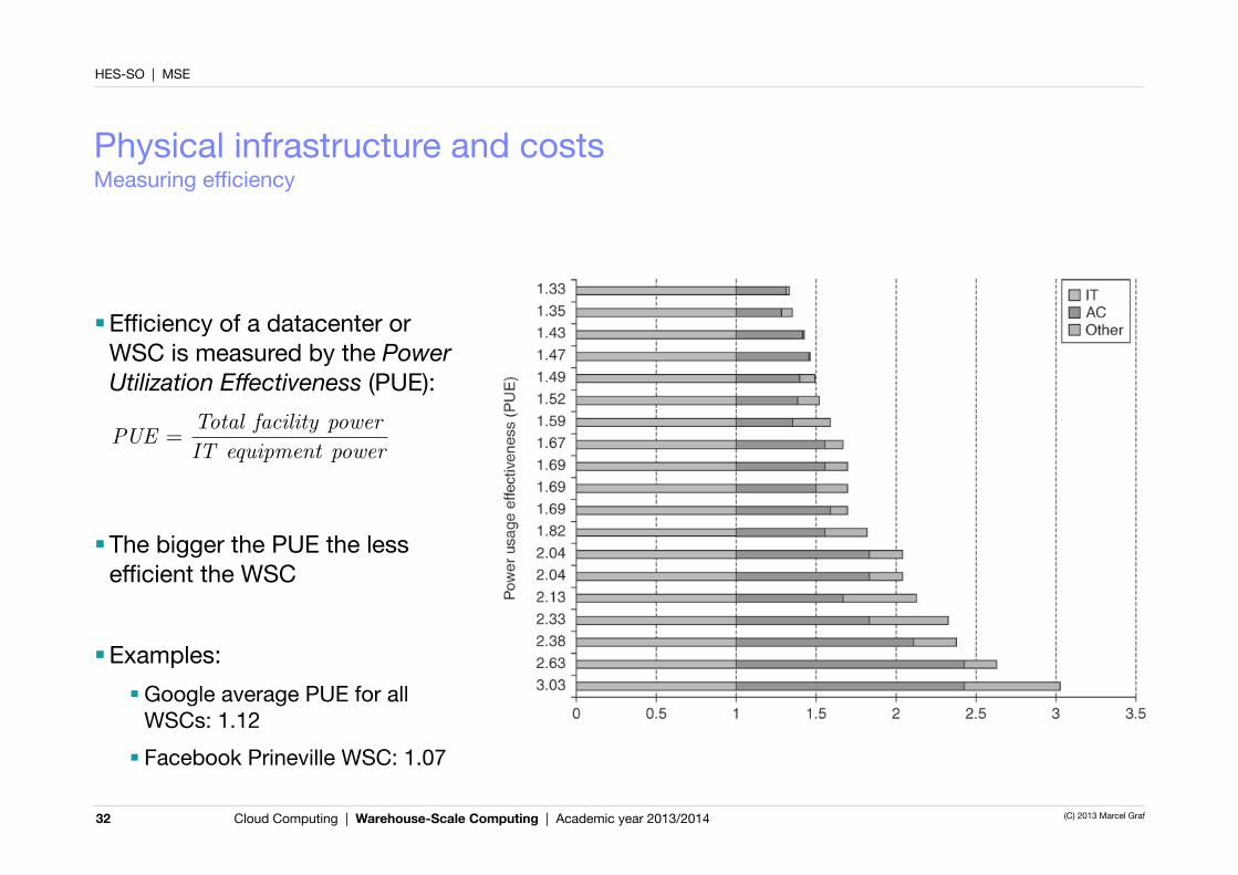
■Efficiency of a datacenter or WSC is measured by the Power Utilization Effectiveness (PUE):

■The bigger the PUE the less efficient the WSC

■Examples:■Google average PUE for all

WSCs: 1.12■ Facebook Prineville WSC: 1.07

PUE =Total facility power

IT equipment power

HES-SO | MSE


Physical infrastructure and costsMeasuring efficiency

33

Google WSC historical performance Facebook WSC performance dashboard

HES-SO | MSE


Physical infrastructure and costsCost

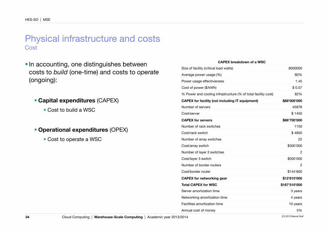
■ In accounting, one distinguishes between costs to build (one-time) and costs to operate (ongoing):

■Capital expenditures (CAPEX)■ Cost to build a WSC

■Operational expenditures (OPEX)■ Cost to operate a WSC

34

CAPEX breakdown of a WSCCAPEX breakdown of a WSCSize of facility (critical load watts) 8000000

Average power usage (%) 80%

Power usage effectivieness 1.45

Cost of power ($/kWh) $ 0.07

% Power and cooling infrastructure (% of total facility cost) 82%

CAPEX for facility (not including IT equipment) $88'000'000Number of servers 45978

Cost/server $ 1450

CAPEX for servers $66'700'000Number of rack switches 1150

Cost/rack switch $ 4800

Number of array switches 22

Cost/array switch $300'000

Number of layer 3 switches 2

Cost/layer 3 switch $500'000

Number of border routers 2

Cost/border router $144'800

CAPEX for networking gear $12'810'000

Total CAPEX for WSC $167'510'000Server amortization time 3 years

Networking amortization time 4 years

Facilities amortization time 10 years

Annual cost of money 5%

HES-SO | MSE


Physical infrastructure and costsCost

35

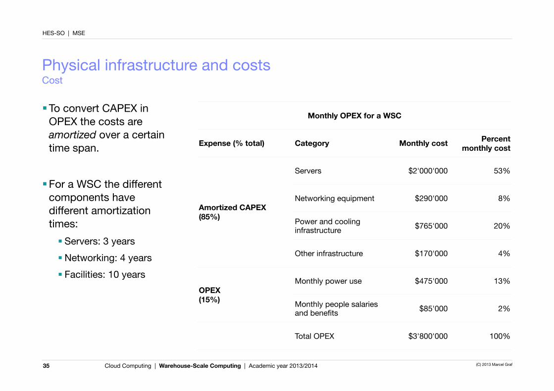
Monthly OPEX for a WSCMonthly OPEX for a WSCMonthly OPEX for a WSCMonthly OPEX for a WSC

Expense (% total) Category Monthly cost Percent monthly cost

Amortized CAPEX(85%)

Servers $2'000'000 53%


Networking equipment $290'000 8%Amortized CAPEX(85%) Power and cooling

infrastructure $765'000 20%


Other infrastructure $170'000 4%

OPEX (15%)

Monthly power use $475'000 13%OPEX (15%) Monthly people salaries

and benefits $85'000 2%

Total OPEX $3'800'000 100%

■To convert CAPEX in OPEX the costs are amortized over a certain time span.

■For a WSC the different components have different amortization times:■ Servers: 3 years■Networking: 4 years■ Facilities: 10 years

HES-SO | MSE


Physical infrastructure and costsEconomies of scale

■WSCs offer economies of scale that cannot be achieved with a datacenter. Compared to a 1'000-server datacenter a WSC has the following advantages (2006 study):■ 5.7 times reduction in storage costs

■ Datacenter: $26 per GB-year, WSC: $4.6 per GB-year

■ 7.1 times reduction in administrative costs■ Datacenter: 140 servers per administrator, WSC: over 1000 per administrator

■ 7.3 times reduction in networking costs■ Datacenter: $95 per Mbit/s per month, WSC: $13 per Mbit/s per month

■This makes cloud services economically attractive.

36

HES-SO | MSE


Exercise 04.01

■Software that runs in WSCs often uses replication to overcome failures. For example the file system of Hadoop, HDFS, employs three-way replication (one local copy, one remote copy in the rack and one remote copy in a separate rack), as do many NoSQL databases.

■A survey among attendees of the Hadoop World 2010 conference showed that most Hadoop clusters have 10 machines or less, with dataset sizes of 10 TB or less. Using Google's numbers for observed outages and anomalies (p. 18), what kind of availability does a 10-node Hadoop cluster have with one-, two-, and three-way replication? Express the availability in number of nines.■ Use the approach on page 20 to calculate the availability with one-way (i.e. no) replication by scaling the

observed 2400-machine cluster to a 10-machine cluster.■ When considering disk failures we are only interested in their impact on availability, ignore the data loss for this

exercise.

■ Then calculate the availability for two-way and three-way replication.

■Google and Facebook are known to use much bigger clusters for their Big Data analytics. What are the availability numbers for a 1000-machine cluster with one-, two-, and three-way replication?

37

HES-SO | MSE


Acknowledgements

■Many charts are based on the book "Computer Architecture — A Quantitative Approach" by John Hennessy and David Patterson, 5th edition, Morgan Kaufmann, 2013

38

cloud lc04 warehouse-scale...

Documents