clouds and the earth's radiant energy system (ceres) data
TRANSCRIPT
Clouds and the Earth's Radiant Energy System(CERES)
Data Management System
DRAFT ES-8 Collection Guide
Release 3Version 4
Primary Authors
Lee-hwa Chang, John L. Robbins
Science Applications International Corporation (SAIC)One Enterprise Parkway, Suite 300
Hampton, VA 23666-5845
Richard N. Green, James F. Kibler
NASA Langley Research CenterClimate Science Branch
Science DirectorateBuilding 1250
21 Langley BoulevardHampton, VA 23681-2199
January 2003
DRAFT ES-8 Collection Guide 2/1/2006
ii
Document Revision Record
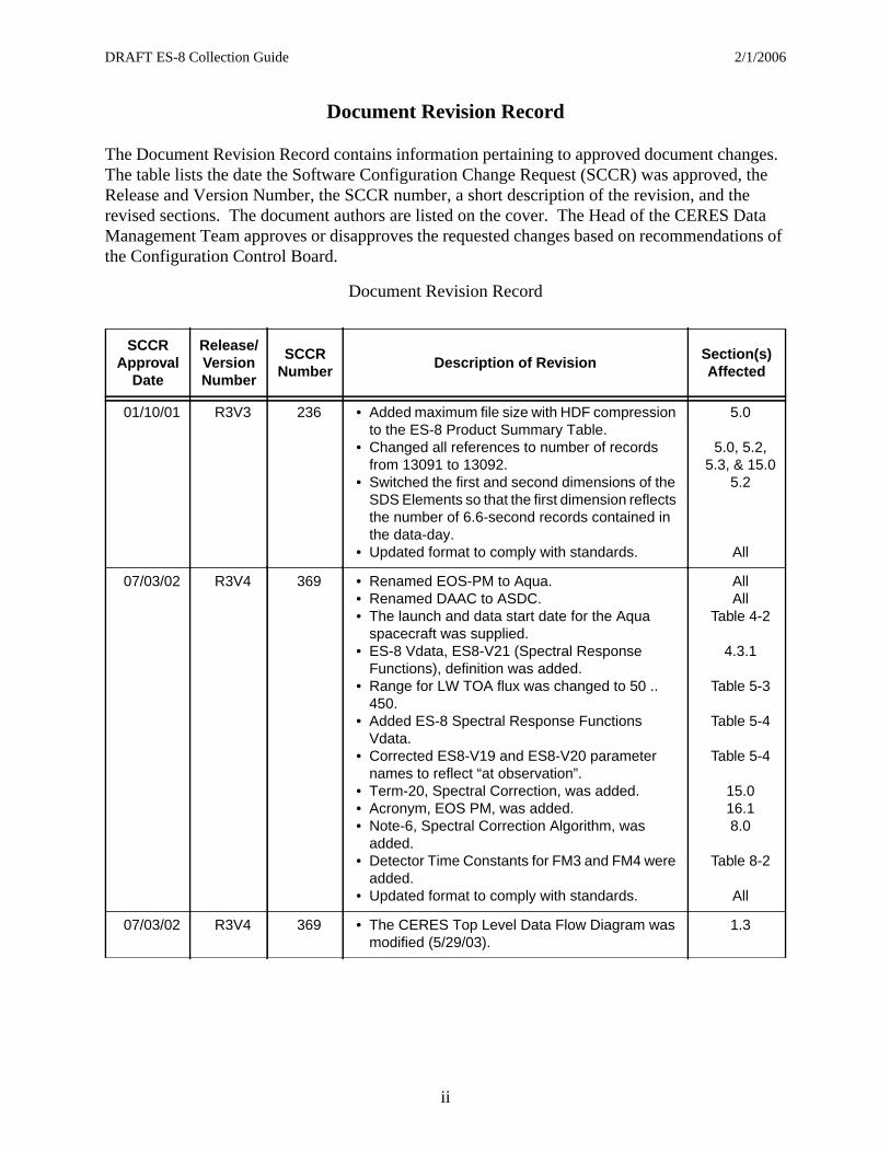
The Document Revision Record contains information pertaining to approved document changes. The table lists the date the Software Configuration Change Request (SCCR) was approved, the Release and Version Number, the SCCR number, a short description of the revision, and the revised sections. The document authors are listed on the cover. The Head of the CERES Data Management Team approves or disapproves the requested changes based on recommendations of the Configuration Control Board.
Document Revision Record
SCCRApproval
Date
Release/VersionNumber
SCCRNumber
Description of Revision Section(s)Affected
01/10/01 R3V3 236 • Added maximum file size with HDF compression to the ES-8 Product Summary Table.
• Changed all references to number of records from 13091 to 13092.
• Switched the first and second dimensions of the SDS Elements so that the first dimension reflects the number of 6.6-second records contained in the data-day.
• Updated format to comply with standards.
5.0
5.0, 5.2, 5.3, & 15.0
5.2
All
07/03/02 R3V4 369 • Renamed EOS-PM to Aqua.• Renamed DAAC to ASDC.• The launch and data start date for the Aqua
spacecraft was supplied.• ES-8 Vdata, ES8-V21 (Spectral Response
Functions), definition was added.• Range for LW TOA flux was changed to 50 ..
450.• Added ES-8 Spectral Response Functions
Vdata.• Corrected ES8-V19 and ES8-V20 parameter
names to reflect “at observation”.• Term-20, Spectral Correction, was added.• Acronym, EOS PM, was added.• Note-6, Spectral Correction Algorithm, was
added.• Detector Time Constants for FM3 and FM4 were
added.• Updated format to comply with standards.
AllAll
Table 4-2
4.3.1
Table 5-3
Table 5-4
Table 5-4
15.016.18.0
Table 8-2
All
07/03/02 R3V4 369 • The CERES Top Level Data Flow Diagram was modified (5/29/03).
1.3

DRAFT ES-8 Collection Guide 2/1/2006
iii
Preface
The Clouds and the Earth’s Radiant Energy System (CERES) Data Management System supports the data processing needs of the CERES Science Team research to increase understanding of the Earth’s climate and radiant environment. The CERES Data Management Team works with the CERES Science Team to develop the software necessary to implement the science algorithms. This software, being developed to operate at the Langley Atmospheric Sciences Data Center (ASDC), produces an extensive set of science data products.
The Data Management System consists of 12 subsystems; each subsystem represents one or more stand-alone executable programs. Each subsystem executes when all of its required input data sets are available and produces one or more archival science products.
This Collection Guide is intended to give an overview of the science product along with definitions of each of the parameters included within the product. The document has been reviewed by the CERES Working Group teams responsible for producing the product and by the Working Group Teams who use the product.
Acknowledgment is given to Tammy O. Ayers and Thanh Duong of Science Applications International Corporation (SAIC) for their support in the preparation of this document.
DRAFT ES-8 Collection Guide 2/1/2006
TABLE OF CONTENTSSection Page
iv
Preface . . . . . . . . . . . . . . . . . . . . . . . . . . . . . . . . . . . . . . . . . . . . . . . . . . . . . . . . . . . . . . . . . . . . . iii
Summary . . . . . . . . . . . . . . . . . . . . . . . . . . . . . . . . . . . . . . . . . . . . . . . . . . . . . . . . . . . . . . . . . . . . 1
1.0 Collection Overview . . . . . . . . . . . . . . . . . . . . . . . . . . . . . . . . . . . . . . . . . . . . . . . . . . . . . . 1
1.1 Collection Identification . . . . . . . . . . . . . . . . . . . . . . . . . . . . . . . . . . . . . . . . . . . . . 1
1.2 Collection Introduction . . . . . . . . . . . . . . . . . . . . . . . . . . . . . . . . . . . . . . . . . . . . . . 2
1.3 Objective/Purpose . . . . . . . . . . . . . . . . . . . . . . . . . . . . . . . . . . . . . . . . . . . . . . . . . . 2
1.4 Summary of Parameters . . . . . . . . . . . . . . . . . . . . . . . . . . . . . . . . . . . . . . . . . . . . . 5
1.5 Discussion . . . . . . . . . . . . . . . . . . . . . . . . . . . . . . . . . . . . . . . . . . . . . . . . . . . . . . . . 5
1.6 Related Collections . . . . . . . . . . . . . . . . . . . . . . . . . . . . . . . . . . . . . . . . . . . . . . . . . 5
2.0 Investigators . . . . . . . . . . . . . . . . . . . . . . . . . . . . . . . . . . . . . . . . . . . . . . . . . . . . . . . . . . . . 6
2.1 Title of Investigation . . . . . . . . . . . . . . . . . . . . . . . . . . . . . . . . . . . . . . . . . . . . . . . 6
2.2 Contact Information . . . . . . . . . . . . . . . . . . . . . . . . . . . . . . . . . . . . . . . . . . . . . . . . 6
3.0 Origination . . . . . . . . . . . . . . . . . . . . . . . . . . . . . . . . . . . . . . . . . . . . . . . . . . . . . . . . . . . . . 7
4.0 Data Description . . . . . . . . . . . . . . . . . . . . . . . . . . . . . . . . . . . . . . . . . . . . . . . . . . . . . . . . . 8
4.1 Spatial Characteristics. . . . . . . . . . . . . . . . . . . . . . . . . . . . . . . . . . . . . . . . . . . . . . . 8
4.1.1 Spatial Coverage . . . . . . . . . . . . . . . . . . . . . . . . . . . . . . . . . . . . . . . . . . . . . 8
4.1.2 Spatial Resolution . . . . . . . . . . . . . . . . . . . . . . . . . . . . . . . . . . . . . . . . . . . . 8
4.2 Temporal Characteristics . . . . . . . . . . . . . . . . . . . . . . . . . . . . . . . . . . . . . . . . . . . . 8
4.2.1 Temporal Coverage. . . . . . . . . . . . . . . . . . . . . . . . . . . . . . . . . . . . . . . . . . . 8
4.2.2 Temporal Resolution. . . . . . . . . . . . . . . . . . . . . . . . . . . . . . . . . . . . . . . . . . 9
4.3 Parameter Definitions . . . . . . . . . . . . . . . . . . . . . . . . . . . . . . . . . . . . . . . . . . . . . . . 9
4.3.1 ES-8 Vdata . . . . . . . . . . . . . . . . . . . . . . . . . . . . . . . . . . . . . . . . . . . . . . . . . 9
4.3.2 ES-8 Scientific Data Definitions. . . . . . . . . . . . . . . . . . . . . . . . . . . . . . . . 13
4.4 Fill Values. . . . . . . . . . . . . . . . . . . . . . . . . . . . . . . . . . . . . . . . . . . . . . . . . . . . . . . 28
4.5 Sample Data File. . . . . . . . . . . . . . . . . . . . . . . . . . . . . . . . . . . . . . . . . . . . . . . . . . 28
5.0 Data Organization . . . . . . . . . . . . . . . . . . . . . . . . . . . . . . . . . . . . . . . . . . . . . . . . . . . . . . . 29
5.1 Data Granularity . . . . . . . . . . . . . . . . . . . . . . . . . . . . . . . . . . . . . . . . . . . . . . . . . . 30
5.2 ES-8 HDF Scientific Data Sets (SDS) . . . . . . . . . . . . . . . . . . . . . . . . . . . . . . . . . 30
5.3 ES-8 HDF Vertex Data (Vdata) . . . . . . . . . . . . . . . . . . . . . . . . . . . . . . . . . . . . . . 31
5.4 ES-8 Metadata. . . . . . . . . . . . . . . . . . . . . . . . . . . . . . . . . . . . . . . . . . . . . . . . . . . . 32
6.0 Theory of Measurements and Data Manipulations. . . . . . . . . . . . . . . . . . . . . . . . . . . . . . 33
6.1 Theory of Measurements . . . . . . . . . . . . . . . . . . . . . . . . . . . . . . . . . . . . . . . . . . . 33
6.2 Data Processing Sequence . . . . . . . . . . . . . . . . . . . . . . . . . . . . . . . . . . . . . . . . . . 33
6.3 Special Corrections/Adjustments . . . . . . . . . . . . . . . . . . . . . . . . . . . . . . . . . . . . . 33
7.0 Errors. . . . . . . . . . . . . . . . . . . . . . . . . . . . . . . . . . . . . . . . . . . . . . . . . . . . . . . . . . . . . . . . . 34
DRAFT ES-8 Collection Guide 2/1/2006
TABLE OF CONTENTSSection Page
v
7.1 Quality Assessment. . . . . . . . . . . . . . . . . . . . . . . . . . . . . . . . . . . . . . . . . . . . . . . . 34
7.2 Data Validation by Source . . . . . . . . . . . . . . . . . . . . . . . . . . . . . . . . . . . . . . . . . . 34
8.0 Notes . . . . . . . . . . . . . . . . . . . . . . . . . . . . . . . . . . . . . . . . . . . . . . . . . . . . . . . . . . . . . . . . . 35
Note-1 Conversion of Julian Date to Calendar Date. . . . . . . . . . . . . . . . . . . . . . . . . . 35
Note-2 Colatitude and Longitude of Nadir . . . . . . . . . . . . . . . . . . . . . . . . . . . . . . . . . 38
Note-3 CERES Point Spread Function . . . . . . . . . . . . . . . . . . . . . . . . . . . . . . . . . . . . 39
Note-4 Definition of Angular Distribution Models (ADM) . . . . . . . . . . . . . . . . . . . . 44
Note-5 Maximum Likelihood Estimator (MLE) of Scene Type. . . . . . . . . . . . . . . . . 45
Note-6 Spectral Correction Algorithm . . . . . . . . . . . . . . . . . . . . . . . . . . . . . . . . . . . . 46
9.0 Application of the Data Set. . . . . . . . . . . . . . . . . . . . . . . . . . . . . . . . . . . . . . . . . . . . . . . . 48
10.0 Future Modifications and Plans . . . . . . . . . . . . . . . . . . . . . . . . . . . . . . . . . . . . . . . . . . . . 48
11.0 Software Description . . . . . . . . . . . . . . . . . . . . . . . . . . . . . . . . . . . . . . . . . . . . . . . . . . . . 48
12.0 Contact Data Center/Obtain Data . . . . . . . . . . . . . . . . . . . . . . . . . . . . . . . . . . . . . . . . . . . 48
13.0 Output Products and Availability . . . . . . . . . . . . . . . . . . . . . . . . . . . . . . . . . . . . . . . . . . . 48
14.0 References. . . . . . . . . . . . . . . . . . . . . . . . . . . . . . . . . . . . . . . . . . . . . . . . . . . . . . . . . . . . . 49
15.0 Glossary of Terms. . . . . . . . . . . . . . . . . . . . . . . . . . . . . . . . . . . . . . . . . . . . . . . . . . . . . . . 50
16.0 Acronyms and Units . . . . . . . . . . . . . . . . . . . . . . . . . . . . . . . . . . . . . . . . . . . . . . . . . . . . . 54
16.1 CERES Acronyms . . . . . . . . . . . . . . . . . . . . . . . . . . . . . . . . . . . . . . . . . . . . . . . . 54
16.2 CERES Units . . . . . . . . . . . . . . . . . . . . . . . . . . . . . . . . . . . . . . . . . . . . . . . . . . . . 56
17.0 Document Information . . . . . . . . . . . . . . . . . . . . . . . . . . . . . . . . . . . . . . . . . . . . . . . . . . . 58
17.1 Document Creation Date - May 15, 1998. . . . . . . . . . . . . . . . . . . . . . . . . . . . . . . 58
17.2 Document Review Date - . . . . . . . . . . . . . . . . . . . . . . . . . . . . . . . . . . . . . . . . . . . 58
17.3 Document Revision Date . . . . . . . . . . . . . . . . . . . . . . . . . . . . . . . . . . . . . . . . . . . 58
17.4 Document ID. . . . . . . . . . . . . . . . . . . . . . . . . . . . . . . . . . . . . . . . . . . . . . . . . . . . . 58
17.5 Citation . . . . . . . . . . . . . . . . . . . . . . . . . . . . . . . . . . . . . . . . . . . . . . . . . . . . . . . . . 58
17.6 Redistribution of Data. . . . . . . . . . . . . . . . . . . . . . . . . . . . . . . . . . . . . . . . . . . . . . 58
17.7 Document Curator. . . . . . . . . . . . . . . . . . . . . . . . . . . . . . . . . . . . . . . . . . . . . . . . . 58
18.0 Index . . . . . . . . . . . . . . . . . . . . . . . . . . . . . . . . . . . . . . . . . . . . . . . . . . . . . . . . . . . . . . . . 59
APPENDIX A CERES Metadata . . . . . . . . . . . . . . . . . . . . . . . . . . . . . . . . . . . . . . . . . . . . . . . . A-1
DRAFT ES-8 Collection Guide 2/1/2006
LIST OF TABLESTable Page
vi
Table 3-1. CERES Instruments . . . . . . . . . . . . . . . . . . . . . . . . . . . . . . . . . . . . . . . . . . . . . . . . 7
Table 4-1. ES-8 Spatial Coverage . . . . . . . . . . . . . . . . . . . . . . . . . . . . . . . . . . . . . . . . . . . . . . 8
Table 4-2. CERES Temporal Coverage . . . . . . . . . . . . . . . . . . . . . . . . . . . . . . . . . . . . . . . . . . 8
Table 4-3. CERES Orbit Characteristics . . . . . . . . . . . . . . . . . . . . . . . . . . . . . . . . . . . . . . . . . 9
Table 4-4. ERBE Scene Types . . . . . . . . . . . . . . . . . . . . . . . . . . . . . . . . . . . . . . . . . . . . . . . . 20
Table 4-5. Bit Order for Radiometric and FOV Quality Flags . . . . . . . . . . . . . . . . . . . . . . . 21
Table 4-6. Scanner Operations Flag Word 1 (of 3) . . . . . . . . . . . . . . . . . . . . . . . . . . . . . . . . 22
Table 4-7. Scanner Operations Flag Word 2 (of 3) . . . . . . . . . . . . . . . . . . . . . . . . . . . . . . . . 23
Table 4-8. Scanner Operations Flag Word 3 (of 3) . . . . . . . . . . . . . . . . . . . . . . . . . . . . . . . . 24
Table 4-9. CERES Fill Values . . . . . . . . . . . . . . . . . . . . . . . . . . . . . . . . . . . . . . . . . . . . . . . . 28
Table 5-1. ES-8 Product Summary. . . . . . . . . . . . . . . . . . . . . . . . . . . . . . . . . . . . . . . . . . . . . 29
Table 5-2. ES-8 Product Specific Metadata . . . . . . . . . . . . . . . . . . . . . . . . . . . . . . . . . . . . . . 29
Table 5-3. ES-8 SDS Summary (1 of 2) . . . . . . . . . . . . . . . . . . . . . . . . . . . . . . . . . . . . . . . . 30
Table 5-4. ES-8 Vdata Summary (1 of 2) . . . . . . . . . . . . . . . . . . . . . . . . . . . . . . . . . . . . . . . 31
Table 8-1. Julian Day Number . . . . . . . . . . . . . . . . . . . . . . . . . . . . . . . . . . . . . . . . . . . . . . . . 37
Table 8-2. Detector Time Constant (t seconds) . . . . . . . . . . . . . . . . . . . . . . . . . . . . . . . . . . . 41
Table A-1. CERES Baseline Header Metadata (1 of 2) . . . . . . . . . . . . . . . . . . . . . . . . . . . . A-1
Table A-2. CERES_metadata Vdata . . . . . . . . . . . . . . . . . . . . . . . . . . . . . . . . . . . . . . . . . . . A-3

DRAFT ES-8 Collection Guide 2/1/2006
LIST OF FIGURESFigure Page
vii
Figure 1-1. CERES Top Level Data Flow Diagram . . . . . . . . . . . . . . . . . . . . . . . . . . . . . . . . . 4
Figure 4-1. Colatitude and Longitude . . . . . . . . . . . . . . . . . . . . . . . . . . . . . . . . . . . . . . . . . . . 12
Figure 4-2. Viewing Angles at TOA . . . . . . . . . . . . . . . . . . . . . . . . . . . . . . . . . . . . . . . . . . . . 16
Figure 8-1. Scanner Footprint Geometry. . . . . . . . . . . . . . . . . . . . . . . . . . . . . . . . . . . . . . . . . 39
Figure 8-2. Optical FOV . . . . . . . . . . . . . . . . . . . . . . . . . . . . . . . . . . . . . . . . . . . . . . . . . . . . . 40
Figure 8-3. TRMM Angular Bin Weights . . . . . . . . . . . . . . . . . . . . . . . . . . . . . . . . . . . . . . . . 43
Figure 8-4. ERBE Scene Identification Algorithm . . . . . . . . . . . . . . . . . . . . . . . . . . . . . . . . . 45
Figure 8-5. CERES_TRMM Spectral Response . . . . . . . . . . . . . . . . . . . . . . . . . . . . . . . . . . . 47
Figure 15-1. Cone Angle . . . . . . . . . . . . . . . . . . . . . . . . . . . . . . . . . . . . . . . . . . . . . . . . . . . . . . 50
Figure 15-2. Ellipsoidal Model . . . . . . . . . . . . . . . . . . . . . . . . . . . . . . . . . . . . . . . . . . . . . . . . . 50
Figure 15-3. Normal and short Earth scan profiles for instrument on TRMM platform. . . . . . 52
DRAFT ES-8 Collection Guide 2/1/2006
Collection Overview 1
Clouds and the Earth's Radiant Energy System (CERES)ES-8 Collection Guide
Summary
CERES is a key component of the EOS program. The CERES instrument provides radiometric measurements of the Earth's atmosphere from three broadband channels: a shortwave channel (0.3 - 5 µm), a total channel (0.3 - 200 µm), and an infrared window channel (8 - 12 µm). The CERES instruments are improved models of the ERBE scanner instruments, which operated from 1984 through 1990 on NASA’s ERBS and on NOAA’s operational weather satellites, NOAA-9 and NOAA-10. The strategy of flying instruments on Sun-synchronous, polar orbiting satellites, such as NOAA-9 and NOAA-10, simultaneously with instruments on satellites that have precessing orbits in lower inclinations, such as ERBS, was successfully developed in ERBE to reduce time sampling errors. CERES continues that strategy by flying instruments on the polar orbiting EOS platforms simultaneously with an instrument on the TRMM spacecraft, which has an orbital inclination of 35 degrees. The TRMM satellite carries one CERES instrument while the Terra and Aqua EOS satellites carry two CERES instruments, one operating in a FAPS mode for continuous Earth sampling and the other operating in a RAPS mode for improved angular sampling.
To preserve historical continuity, some parts of the CERES data reduction use algorithms identical with the algorithms used in ERBE. At the same time, many of the algorithms on CERES are new. To reduce the uncertainty in data interpretation and to improve the consistency between the cloud parameters and the radiation fields, CERES includes cloud imager data and other atmospheric parameters. The CERES investigation is designed to monitor the top-of-atmosphere radiation budget as defined by ERBE, to define the physical properties of clouds, to define the surface radiation budget, and to determine the divergence of energy throughout the atmosphere. The CERES DMS produces products which support research to increase understanding of the Earth’s climate and radiant environment.
The ES-8 archival data product was created as an HDF-EOS (See Reference 1) swath data structure and contains a 24-hour, single-satellite, instantaneous view of scanner fluxes at the TOA (See Term-22) reduced from spacecraft altitude unfiltered radiances using the ERBE scanner Inversion algorithms and the ERBE SW and LW ADMs. The ES-8 also includes the TOT, SW, and WN channel radiometric data; SW, LW, and WN unfiltered radiance values; and the ERBE scene identification for each measurement. These data are organized according to the CERES 3.3-second scan into 6.6-second records. As long as there is one valid scanner measurement within a record, the ES-8 record will be generated.
1.0 Collection Overview
1.1 Collection Identification
The ES-8 filename is

DRAFT ES-8 Collection Guide 2/1/2006
Collection Overview 2
CER_ ES8_Sampling-Strategy_Production-Strategy_XXXXXX.YYYYMMDD where
CER Investigation designation for CERES,ES8 Product identification for the primary science data product (external
distribution),Sampling-Strategy Platform, instrument, and imager (e.g., TRMM-PFM-VIRS),Production-Strategy Edition or campaign (e.g., At-launch, ValidationR1, Edition1),XXXXXX Configuration code for file and software version management,YYYY 4-digit integer defining data acquisition year,MM 2-digit integer defining data acquisition month, andDD 2-digit integer defining the data acquisition day.
1.2 Collection Introduction
The ES-8 data product is a Level-2 archival product that contains a 24-hour, single-satellite, single-instrument, instantaneous view of scanner fluxes at the TOA reduced from spacecraft altitude unfiltered radiances using the ERBE scanner Inversion algorithms and the ERBE SW and LW ADMs.
1.3 Objective/Purpose
The overall science objectives of the CERES investigation are
1. For climate change research, provide a continuation of the ERBE radiative fluxes at the TOA that are analyzed using the same techniques used with existing ERBE data.
2. Double the accuracy of estimates of radiative fluxes at the TOA and the Earth’s surface from existing ERBE data.
3. Provide the first long-term global estimates of the radiative fluxes within the Earth’s atmosphere.
4. Provide cloud property estimates which are consistent with the radiative fluxes from surface to TOA.
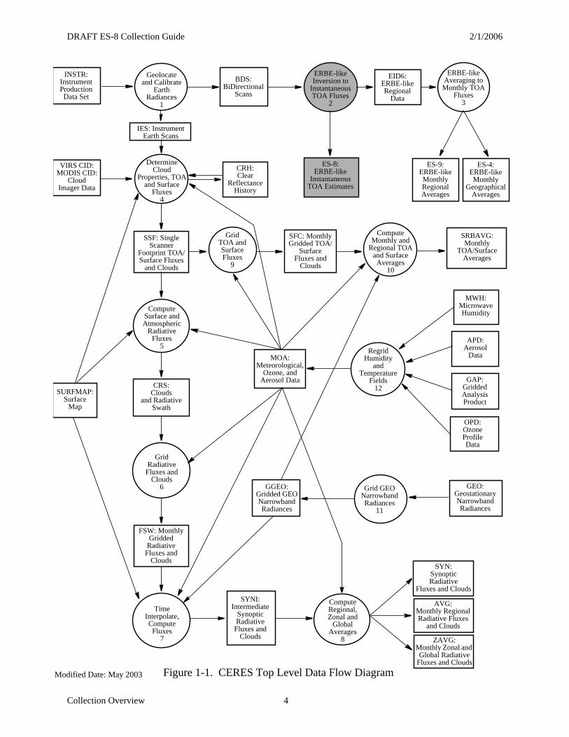
The CERES DMS is a software management and processing system which processes CERES instrument measurements and associated engineering data to produce archival science and other data products. The DMS is executed at the LaRC ASDC, which is also responsible for distributing the data products. A high-level view of the CERES DMS is illustrated by the CERES Top Level Data Flow Diagram shown in Figure 1-1.
Circles in the diagram represent algorithm processes called subsystems, which are a logical collection of algorithms that together convert input products into output products. Boxes represent archival products. Two parallel lines represent data stores which are designated as nonarchival or temporary data products. Boxes or data stores with arrows entering a circle are input sources for the subsystem, while boxes or data stores with arrows exiting the circles are output products.
DRAFT ES-8 Collection Guide 2/1/2006
Collection Overview 3
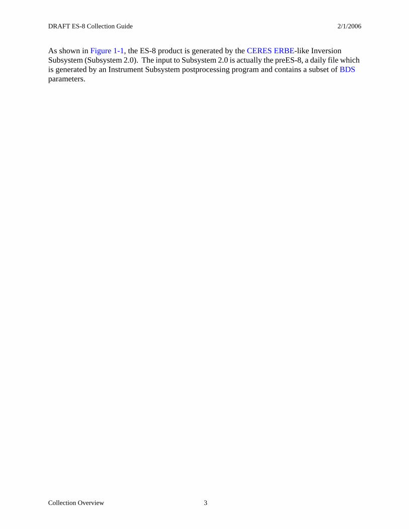
As shown in Figure 1-1, the ES-8 product is generated by the CERES ERBE-like Inversion Subsystem (Subsystem 2.0). The input to Subsystem 2.0 is actually the preES-8, a daily file which is generated by an Instrument Subsystem postprocessing program and contains a subset of BDS parameters.
DRAFT ES-8 Collection Guide 2/1/2006
Collection Overview 4
EID6:ERBE-like Regional
Data
GridTOA andSurfaceFluxes
9
ERBE-likeAveraging to
Monthly TOAFluxes
3
Grid GEONarrowbandRadiances
11
GEO:GeostationaryNarrowbandRadiances
ComputeRegional,Zonal and
GlobalAverages
8
GGEO:Gridded GEONarrowbandRadiances
TimeInterpolate,ComputeFluxes
7
FSW: Monthly Gridded
Radiative Fluxes and
Clouds
Grid Radiative
Fluxes andClouds
6
CRS: Clouds
and RadiativeSwath
ComputeSurface andAtmospheric
RadiativeFluxes
5
MOA:Meteorological,
Ozone, andAerosol Data
SFC: MonthlyGridded TOA/
SurfaceFluxes and
Clouds
SSF: SingleScanner
Footprint TOA/Surface Fluxes
and Clouds
VIRS CID:MODIS CID:
CloudImager Data
ES-8:ERBE-like
InstantaneousTOA Estimates
CRH:Clear
ReflectanceHistory
ERBE-likeInversion to
InstantaneousTOA Fluxes
2
ES-4:ERBE-likeMonthly
Geographical Averages
ES-9:ERBE-likeMonthly Regional Averages
RegridHumidity
andTemperature
Fields12
MWH:MicrowaveHumidity
APD:Aerosol
Data
GAP:Gridded Analysis Product
OPD:OzoneProfileData
INSTR:InstrumentProduction Data Set
Geolocateand Calibrate
EarthRadiances
1
BDS:BiDirectional
Scans
SRBAVG:Monthly
TOA/Surface Averages
SURFMAP:Surface
Map
SYNI:Intermediate
SynopticRadiative
Fluxes and Clouds ZAVG:
Monthly Zonal and Global Radiative
Fluxes and Clouds
ComputeMonthly and
Regional TOAand SurfaceAverages
10
DetermineCloud
Properties, TOAand Surface
Fluxes4
IES: InstrumentEarth Scans
AVG:Monthly RegionalRadiative Fluxes
and Clouds
Figure 1-1. CERES Top Level Data Flow DiagramModified Date: May 2003
SYN:SynopticRadiative
Fluxes and Clouds
DRAFT ES-8 Collection Guide 2/1/2006
Collection Overview 5
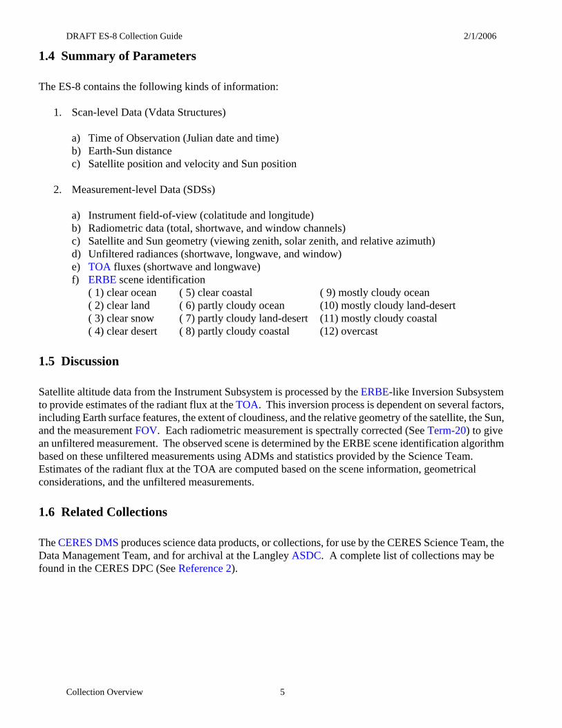
1.4 Summary of Parameters
The ES-8 contains the following kinds of information:
1. Scan-level Data (Vdata Structures)
a) Time of Observation (Julian date and time)b) Earth-Sun distancec) Satellite position and velocity and Sun position
2. Measurement-level Data (SDSs)
a) Instrument field-of-view (colatitude and longitude)b) Radiometric data (total, shortwave, and window channels)c) Satellite and Sun geometry (viewing zenith, solar zenith, and relative azimuth)d) Unfiltered radiances (shortwave, longwave, and window)e) TOA fluxes (shortwave and longwave)f) ERBE scene identification
( 1) clear ocean ( 5) clear coastal ( 9) mostly cloudy ocean( 2) clear land ( 6) partly cloudy ocean (10) mostly cloudy land-desert( 3) clear snow ( 7) partly cloudy land-desert (11) mostly cloudy coastal( 4) clear desert ( 8) partly cloudy coastal (12) overcast
1.5 Discussion
Satellite altitude data from the Instrument Subsystem is processed by the ERBE-like Inversion Subsystem to provide estimates of the radiant flux at the TOA. This inversion process is dependent on several factors, including Earth surface features, the extent of cloudiness, and the relative geometry of the satellite, the Sun, and the measurement FOV. Each radiometric measurement is spectrally corrected (See Term-20) to give an unfiltered measurement. The observed scene is determined by the ERBE scene identification algorithm based on these unfiltered measurements using ADMs and statistics provided by the Science Team. Estimates of the radiant flux at the TOA are computed based on the scene information, geometrical considerations, and the unfiltered measurements.
1.6 Related Collections
The CERES DMS produces science data products, or collections, for use by the CERES Science Team, the Data Management Team, and for archival at the Langley ASDC. A complete list of collections may be found in the CERES DPC (See Reference 2).

DRAFT ES-8 Collection Guide 2/1/2006
Investigators 6
2.0 Investigators
Dr. Bruce A. Wielicki, CERES Principal InvestigatorE-mail: [email protected]: (757) 864-5683FAX: (757) 864-7996Mail Stop 420Atmospheric Sciences CompetencyBuilding 125021 Langley BoulevardNASA Langley Research CenterHampton, VA 23681-2199
2.1 Title of Investigation
Clouds and the Earth’s Radiant Energy System (CERES)ERBE-like Subsystems (Subsystems 2.0 & 3.0)
2.2 Contact Information
Dr. Kory J. Priestley, Subsystem 2.0 Working Group ChairE-mail: [email protected]: (757) 864-8147
Dr. Takmeng Wong, Subsystem 2.0 Working Group Science and Validation AdvisorE-mail: [email protected]: (757) 864-5607
FAX: (757) 864-7996Mail Stop 420Atmospheric Sciences CompetencyBuilding 125021 Langley BoulevardNASA Langley Research CenterHampton, VA 23681-2199
Edward A. Kizer, Subsystem 2.0 Software and Data Management LeadE-mail: [email protected]: (757) 827-4883FAX: (757) 864-7996Science Applications International Corporation (SAIC)One Enterprise Parkway, Suite 300Hampton, VA 23666-5845
DRAFT ES-8 Collection Guide 2/1/2006
Origination 7
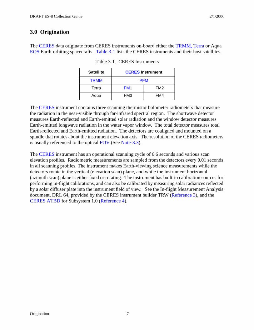
3.0 Origination
The CERES data originate from CERES instruments on-board either the TRMM, Terra or Aqua EOS Earth-orbiting spacecrafts. Table 3-1 lists the CERES instruments and their host satellites.
The CERES instrument contains three scanning thermistor bolometer radiometers that measure the radiation in the near-visible through far-infrared spectral region. The shortwave detector measures Earth-reflected and Earth-emitted solar radiation and the window detector measures Earth-emitted longwave radiation in the water vapor window. The total detector measures total Earth-reflected and Earth-emitted radiation. The detectors are coaligned and mounted on a spindle that rotates about the instrument elevation axis. The resolution of the CERES radiometers is usually referenced to the optical FOV (See Note-3.3).
The CERES instrument has an operational scanning cycle of 6.6 seconds and various scan elevation profiles. Radiometric measurements are sampled from the detectors every 0.01 seconds in all scanning profiles. The instrument makes Earth-viewing science measurements while the detectors rotate in the vertical (elevation scan) plane, and while the instrument horizontal (azimuth scan) plane is either fixed or rotating. The instrument has built-in calibration sources for performing in-flight calibrations, and can also be calibrated by measuring solar radiances reflected by a solar diffuser plate into the instrument field of view. See the In-flight Measurement Analysis document, DRL 64, provided by the CERES instrument builder TRW (Reference 3), and the CERES ATBD for Subsystem 1.0 (Reference 4).
Table 3-1. CERES Instruments
Satellite CERES Instrument
TRMM PFM
Terra FM1 FM2
Aqua FM3 FM4
DRAFT ES-8 Collection Guide 2/1/2006
Data Description 8
4.0 Data Description
4.1 Spatial Characteristics
4.1.1 Spatial Coverage
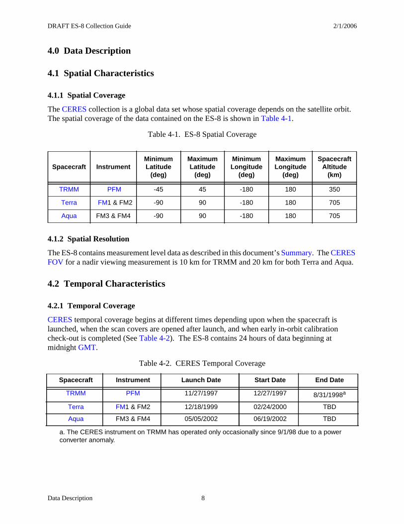
The CERES collection is a global data set whose spatial coverage depends on the satellite orbit. The spatial coverage of the data contained on the ES-8 is shown in Table 4-1.
4.1.2 Spatial Resolution
The ES-8 contains measurement level data as described in this document’s Summary. The CERES FOV for a nadir viewing measurement is 10 km for TRMM and 20 km for both Terra and Aqua.
4.2 Temporal Characteristics
4.2.1 Temporal Coverage
CERES temporal coverage begins at different times depending upon when the spacecraft is launched, when the scan covers are opened after launch, and when early in-orbit calibration check-out is completed (See Table 4-2). The ES-8 contains 24 hours of data beginning at midnight GMT.
Table 4-1. ES-8 Spatial Coverage
Spacecraft InstrumentMinimum Latitude
(deg)
Maximum Latitude
(deg)
Minimum Longitude
(deg)
Maximum Longitude
(deg)
Spacecraft Altitude
(km)
TRMM PFM -45 45 -180 180 350
Terra FM1 & FM2 -90 90 -180 180 705
Aqua FM3 & FM4 -90 90 -180 180 705
Table 4-2. CERES Temporal Coverage
Spacecraft Instrument Launch Date Start Date End Date
TRMM PFM 11/27/1997 12/27/1997 8/31/1998a
a. The CERES instrument on TRMM has operated only occasionally since 9/1/98 due to a power converter anomaly.
Terra FM1 & FM2 12/18/1999 02/24/2000 TBD
Aqua FM3 & FM4 05/05/2002 06/19/2002 TBD
DRAFT ES-8 Collection Guide 2/1/2006
Data Description 9
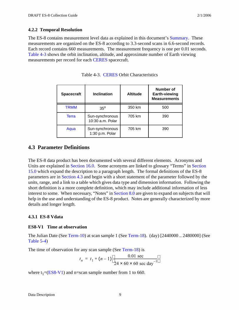
4.2.2 Temporal Resolution
The ES-8 contains measurement level data as explained in this document’s Summary. These measurements are organized on the ES-8 according to 3.3-second scans in 6.6-second records. Each record contains 660 measurements. The measurement frequency is one per 0.01 seconds. Table 4-3 shows the orbit inclination, altitude, and approximate number of Earth viewing measurements per record for each CERES spacecraft.
4.3 Parameter Definitions
The ES-8 data product has been documented with several different elements. Acronyms and Units are explained in Section 16.0. Some acronyms are linked to glossary “Terms” in Section 15.0 which expand the description to a paragraph length. The formal definitions of the ES-8 parameters are in Section 4.3 and begin with a short statement of the parameter followed by the units, range, and a link to a table which gives data type and dimension information. Following the short definition is a more complete definition, which may include additional information of less interest to some. When necessary, “Notes” in Section 8.0 are given to expand on subjects that will help in the use and understanding of the ES-8 product. Notes are generally characterized by more details and longer length.
4.3.1 ES-8 Vdata
ES8-V1 Time at observation
The Julian Date (See Term-10) at scan sample 1 (See Term-18). (day) [2440000 .. 2480000] (See Table 5-4)
The time of observation for any scan sample (See Term-18) is
where t1=(ES8-V1) and n=scan sample number from 1 to 660.
Table 4-3. CERES Orbit Characteristics
Spacecraft Inclination AltitudeNumber of
Earth-viewing Measurements
TRMM 35o 350 km 500
Terra Sun-synchronous10:30 a.m. Polar
705 km 390
Aqua Sun-synchronous1:30 p.m. Polar
705 km 390
tn t1 n 1–( ) 0.01 sec
24 60 60 sec day 1–××-------------------------------------------------------
+=
DRAFT ES-8 Collection Guide 2/1/2006
Data Description 10
In Subsystem 1, the toolkit call PGS_TD_SCtime_to_UTC converts Spacecraft time to UTC time. A second toolkit call, PGS_TD_UTCtoUTCjd, converts the ASCII string into two double precision real numbers, the Julian Date at Greenwich midnight and the fraction of the day since Greenwich midnight, which are added together to obtain the time of observation.
ES8-V2 Earth-Sun distance at record start
The distance from the Earth to the Sun in AU at the scan sample 1 (See Term-18). (AU) [0.98 .. 1.02] (See Table 5-4)
In Subsystem 1, the toolkit call PGS_CBP_CB_Vector computes the Earth-Centered Inertial frame vector to the Sun. The toolkit call PGS_CSC_ECItoECR transforms the position vector to the ECR or Earth equator, Greenwich meridian system (See Term-3). The magnitude of the posi-tion vector is then computed and converted from meters to AU.
ES8-V3 X component of satellite position at record start
The X component of the satellite position at scan sample 1 (See Term-18) in the Earth equator,
Greenwich meridian system (See Term-3). (m) [-8×10⁶ .. 8×10⁶] (See Table 5-4)
In Subsystem 1, the toolkit call PGS_EPH_Earth_EphemAttit computes the satellite position and velocity vector in Earth-Centered Inertial coordinates. A second toolkit call, PGS_CSC_ECItoECR, transforms the position and velocity vector to the ECR or Earth equator, Greenwich meridian system (See Term-3).
ES8-V4 X component of satellite position at record end
The X component of the satellite position at scan sample 660 (See Term-18) in the Earth equator,
Greenwich meridian system (See Term-3). (m) [-8×10⁶ .. 8×10⁶] (See Table 5-4)
The satellite position components are determined from toolkit calls (See ES8-V3).
ES8-V5 Y component of satellite position at record start
The Y component of the satellite position at scan sample 1 (See Term-18) in the Earth equator,
Greenwich meridian system (See Term-3). (m) [-8×10⁶ .. 8×10⁶] (See Table 5-4)
The satellite position components are determined from toolkit calls (See ES8-V3).
ES8-V6 Y component of satellite position at record end
The Y component of the satellite position at scan sample 660 (See Term-18) in the Earth equator,
Greenwich meridian system (See Term-3). (m) [-8×10⁶ .. 8×10⁶] (See Table 5-4)
The satellite position components are determined from toolkit calls (See ES8-V3).
DRAFT ES-8 Collection Guide 2/1/2006
Data Description 11
ES8-V7 Z component of satellite position at record start
The Z component of the satellite position at scan sample 1 (See Term-18) in the Earth equator,
Greenwich meridian system (See Term-3). (m) [-8×10⁶ .. 8×10⁶] (See Table 5-4)
The satellite position components are determined from toolkit calls (See ES8-V3).
ES8-V8 Z component of satellite position at record end
The Z component of the satellite position at scan sample 660 (See Term-18) in the Earth equator,
Greenwich meridian system (See Term-3). (m) [-8×10⁶ .. 8×10⁶] (See Table 5-4)
The satellite position components are determined from toolkit calls (See ES8-V3).
ES8-V9 X component of satellite velocity at record start
The X component of the satellite inertial velocity at scan sample 1 (See Term-18) in the Earth
equator, Greenwich meridian system (See Term-3). (m sec-1) [-1×10⁴ .. 1×10⁴] (See Table 5-4)
The satellite velocity components are determined from toolkit calls (See ES8-V3).
ES8-V10 X component of satellite velocity at record end
The X component of the satellite inertial velocity at scan sample 660 (See Term-18) in the Earth
equator, Greenwich meridian system (See Term-3). (m sec-1) [-1×10⁴ .. 1×10⁴] (See Table 5-4)
The satellite velocity components are determined from toolkit calls (See ES8-V3).
ES8-V11 Y component of satellite velocity at record start
The Y component of the satellite inertial velocity at scan sample 1 (See Term-18) in the Earth
equator, Greenwich meridian system (See Term-3). (m sec-1) [-1×10⁴ .. 1×10⁴] (See Table 5-4)
The satellite velocity components are determined from toolkit calls (See ES8-V3).
ES8-V12 Y component of satellite velocity at record end
The Y component of the satellite inertial velocity at scan sample 660 (See Term-18) in the Earth
equator, Greenwich meridian system (See Term-3). (m sec-1) [-1×10⁴ .. 1×10⁴] (See Table 5-4)
The satellite velocity components are determined from toolkit calls (See ES8-V3).
ES8-V13 Z component of satellite velocity at record start
The Z component of the satellite inertial velocity at scan sample 1 (See Term-18) in the Earth
equator, Greenwich meridian system (See Term-3). (m sec-1) [-1×10⁴ .. 1×10⁴] (See Table 5-4)
The satellite velocity components are determined from toolkit calls (See ES8-V3).
DRAFT ES-8 Collection Guide 2/1/2006
Data Description 12
ES8-V14 Z component of satellite velocity at record end
The Z component of the satellite inertial velocity at scan sample 660 (See Term-18) in the Earth
equator, Greenwich meridian system (See Term-3). (m sec-1) [-1×10⁴ .. 1×10⁴] (See Table 5-4)
The satellite velocity components are determined from toolkit calls (See ES8-V3).
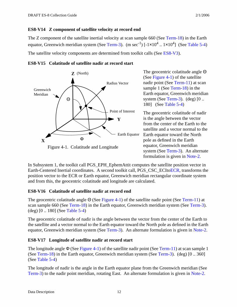
ES8-V15 Colatitude of satellite nadir at record start
The geocentric colatitude angle Θ (See Figure 4-1) of the satellite nadir point (See Term-11) at scan sample 1 (See Term-18) in the Earth equator, Greenwich meridian system (See Term-3). (deg) [0 .. 180] (See Table 5-4)
The geocentric colatitude of nadir is the angle between the vector from the center of the Earth to the satellite and a vector normal to the Earth equator toward the North pole as defined in the Earth equator, Greenwich meridian system (See Term-3). An alternate formulation is given in Note-2.
In Subsystem 1, the toolkit call PGS_EPH_EphemAttit computes the satellite position vector in Earth-Centered Inertial coordinates. A second toolkit call, PGS_CSC_ECItoECR, transforms the position vector to the ECR or Earth equator, Greenwich meridian rectangular coordinate system and from this, the geocentric colatitude and longitude are calculated.
ES8-V16 Colatitude of satellite nadir at record end
The geocentric colatitude angle Θ (See Figure 4-1) of the satellite nadir point (See Term-11) at scan sample 660 (See Term-18) in the Earth equator, Greenwich meridian system (See Term-3). (deg) [0 .. 180] (See Table 5-4)
The geocentric colatitude of nadir is the angle between the vector from the center of the Earth to the satellite and a vector normal to the Earth equator toward the North pole as defined in the Earth equator, Greenwich meridian system (See Term-3). An alternate formulation is given in Note-2.
ES8-V17 Longitude of satellite nadir at record start
The longitude angle Φ (See Figure 4-1) of the satellite nadir point (See Term-11) at scan sample 1 (See Term-18) in the Earth equator, Greenwich meridian system (See Term-3). (deg) [0 .. 360] (See Table 5-4)
The longitude of nadir is the angle in the Earth equator plane from the Greenwich meridian (See Term-3) to the nadir point meridian, rotating East. An alternate formulation is given in Note-2.
Θ
X
Y
Z
Radius Vector
ΦEarth Equator
GreenwichMeridian
Figure 4-1. Colatitude and Longitude
(North)
Point of Interest
DRAFT ES-8 Collection Guide 2/1/2006
Data Description 13
ES8-V18 Longitude of satellite nadir at record end
The longitude angle Φ (See Figure 4-1) of the satellite nadir point (See Term-11) at scan sample 660 (See Term-18) in the Earth equator, Greenwich meridian system (See Term-3). (deg) [0 .. 360] (See Table 5-4)
The longitude of nadir is the angle in the Earth equator plane from the Greenwich meridian (See Term-3) to the nadir point meridian, rotating East. An alternate formulation is given in Note-2.
ES8-V19 Colatitude of Sun at observation
The geocentric colatitude angle of the Sun at scan sample 1 (See Term-18) in the Earth equator, Greenwich meridian system (See Term-3). (deg) [0 .. 180] (See Table 5-4)
The geocentric colatitude of the Sun is the angle between the vector from the center of the Earth to the Sun and a vector normal to the Earth equator toward the North pole as defined in the Earth equator, Greenwich meridian system (See Term-3).
In Subsystem 1, the toolkit call PGS_CBP_Earth_CB_vector computes the sun position vector in Earth-Centered Inertial coordinates. A second toolkit call, PGS_CSC_ECItoECR, transforms the position vector to the ECR or Earth equator, Greenwich meridian rectangular coordinate system and from this, the geocentric colatitude and longitude are calculated.
ES8-V20 Longitude of Sun at observation
The longitude angle of the Sun at scan sample 1 (See Term-18) in the Earth equator, Greenwich meridian system (See Term-3). (deg) [0 .. 360] (See Table 5-4)
The longitude of the Sun is the angle in the Earth equator plane from the Greenwich meridian (See Term-3) to the Sun meridian, rotating East.
ES8-V21 Spectral Response Functions
The spectral response functions are spectral response values (unitless) [0 .. 1] at given wavelengths (microns) for the shortwave, total, and window channels used to create the spectral correction coefficients (See Term-20).
Spectral response function represent the spectral throughput of the detector optical component elements. The spectral response functions are used to spectrally correct the measured radiances that are passed through the optical path of each individual detector to obtain the unfiltered radiances dependent on the scene type (See ES8-14).
4.3.2 ES-8 Scientific Data Definitions
ES8-1 Colatitude of CERES FOV at TOA
This parameter is the geocentric colatitude angle Θ (See Figure 4-1) of the TOA point (See Term-23). (deg) [0 .. 180] (See Table 5-3)
DRAFT ES-8 Collection Guide 2/1/2006
Data Description 14
The geocentric colatitude of the TOA point is the angle between the vector from the center of the Earth to the TOA point (See Term-23) and a vector normal to the Earth equator toward the North pole as defined in the Earth equator, Greenwich meridian system (See Term-3).
If any part of the FOV is off the Earth “surface” (See Term-4), the FOV flag (See ES8-18) is set to bad and the colatitude is set to default. There are 660 values of this parameter per record; one for each measurement point (See Term-17).
In Subsystem 1, the toolkit call PGS_CSC_GetFOV_Pixel returns the geodetic latitude and longitude of the intersection of the FOV centroid and the CERES_TOA model. Another toolkit call PGS_CSC_GEOtoECR transforms the geodetic latitude and longitude to the ECR or Earth equator, Greenwich meridian rectangular coordinates from which the geocentric colatitude and longitude are calculated.
ES8-2 Longitude of CERES FOV at TOA
This parameter is the longitude angle Φ (See Figure 4-1) of the TOA point (See Term-23). (deg) [0 .. 360] (See Table 5-3)
The longitude of the TOA point is the angle in the Earth equator plane from the Greenwich merid-ian (See Term-3) to the TOA point meridian, rotating East.
If any part of the FOV is off the Earth “surface” (See Term-4), the FOV flag (See ES8-18) is set to bad and the longitude is set to default. There are 660 values of this parameter per record; one for each measurement (See Term-17).
The longitude of the TOA point is determined from toolkit calls (See ES8-1).
ES8-3 CERES TOT filtered radiance
This parameter is the measured, spectrally integrated radiance emerging from the TOA, where the spectral integration is weighted by the spectral throughput of the TOT channel. It is the “raw” measurement from the TOT channel after count conversion (See Term-2) and is spectrally corrected (See Term-20) to yield the unfiltered LW radiance (See ES8-10) at night. The TOT and SW filtered radiances are spectrally corrected together to yield the LW radiance during the day.
(W m-2 sr-1) [-2 .. 700] (See Table 5-3)
The value of the filtered TOT radiance is defined as either “good” or “bad” by the quality flag (See ES8-15). If the value is “bad,” for any reason, the TOT filtered radiance is set to a default value (See Section 4.4). If the value is “good,” the measured value is retained. There are 660 values of TOT filtered radiance per record; one for each measurement point (See Term-17).
The TOT filtered radiance is a measure of all radiance that passes through the TOT channel. The spectral weighting produced by the TOT channel throughput is the product of the primary mirror reflectance, the secondary mirror reflectance, and the absorptance of the detector flake. The TOT spectral throughput passes about 90% of the radiant power with wavelengths longer than 5 µm and about 85% of the power with shorter wavelengths.
DRAFT ES-8 Collection Guide 2/1/2006
Data Description 15
ES8-4 CERES SW filtered radiance
This parameter is the measured, spectrally integrated radiance emerging from the TOA, where the spectral integration is weighted by the spectral throughput of the SW channel. It is the “raw” measurement from the SW channel after count conversion (See Term-2) and is spectrally
corrected (See Term-20) to yield the unfiltered SW radiance (See ES8-9). (W m-2 sr-1) [-4 .. 510] (See Table 5-3)
The value of the SW filtered radiance is defined as either “good” or “bad” by the quality flag (See ES8-16). If the value is “bad,” for any reason, the SW filtered radiance is set to a default value (See Section 4.4). If the value is “good” the measured value is retained. There are 660 values of SW filtered radiance per record; one for each measurement point (See Term-17).
The SW filtered radiance is a measure of all radiance that passes through the SW channel. The spectral weighting produced by the SW channel throughput is the product of the SW filter throughput and the TOT channel throughput (See ES8-3). The SW spectral throughput passes about 75% of the radiant power with wavelengths shorter than 5 µm and cuts off rather sharply at about 5 µm. Wavelengths longer than this wavelength contribute a very small fraction of this measurement.
ES8-5 CERES WN filtered radiance
This parameter is a measured, spectrally integrated radiance emerging from the TOA, where the spectral integration is weighted by the spectral throughput of the WN channel. It has a bandpass from approximately 8 to 12 µm. It is the “raw” measurement from the window channel after count conversion (See Term-2) and is spectrally corrected (See Term-20) to yield the unfiltered
WN radiance (See ES8-11). (W m-2 sr-1µm-1) [-1 .. 15] (See Table 5-3)
The value of the WN filtered radiance is defined as either “good” or “bad” by the quality flag (See ES8-17). If the value is “bad,” for any reason, the WN filtered radiance is set to a default value (See Section 4.4). If the value is “good,” the measured value is retained. There are 660 values of WN filtered radiance per record; one for each measurement point (See Term-17).
The WN filtered radiance is a measure of all radiance that passes through the WN channel. The spectral weighting produced by the WN channel throughput is the product of the WN filter throughput and the TOT channel throughput (See ES8-3). The WN spectral throughput passes about 67% of the radiant power between 8 to 12 µm.
DRAFT ES-8 Collection Guide 2/1/2006
Data Description 16
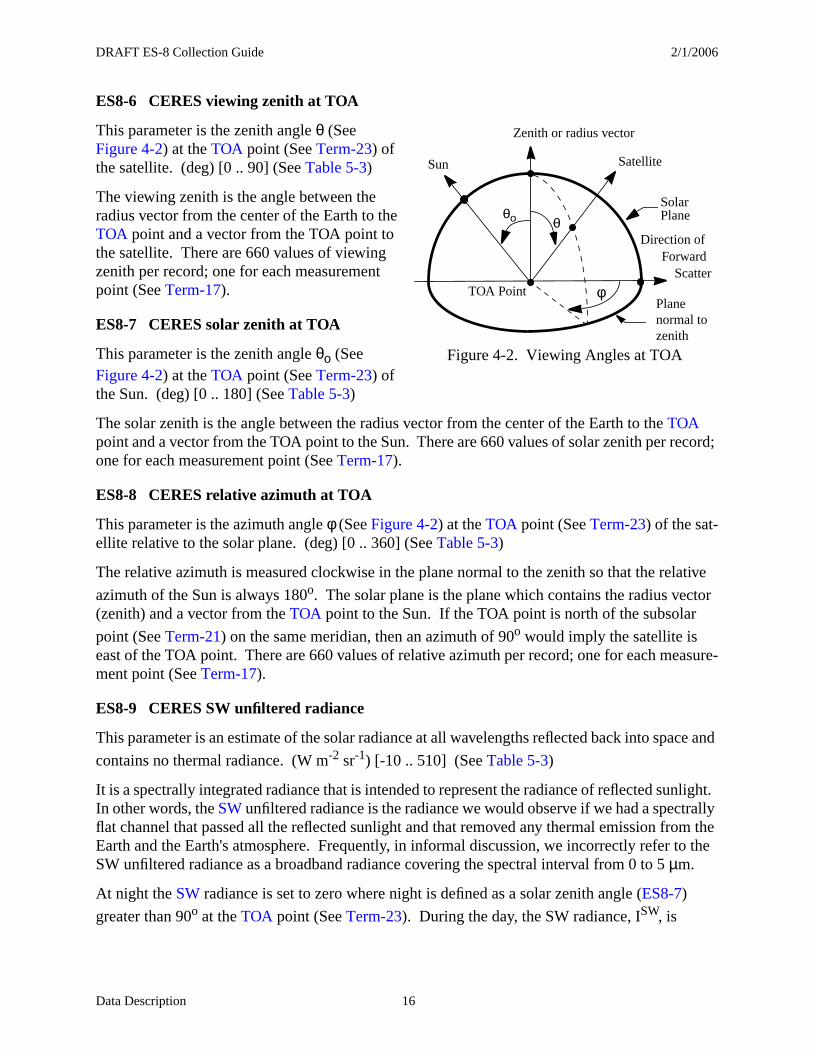
ES8-6 CERES viewing zenith at TOA
This parameter is the zenith angle θ (See Figure 4-2) at the TOA point (See Term-23) of the satellite. (deg) [0 .. 90] (See Table 5-3)
The viewing zenith is the angle between the radius vector from the center of the Earth to the TOA point and a vector from the TOA point to the satellite. There are 660 values of viewing zenith per record; one for each measurement point (See Term-17).
ES8-7 CERES solar zenith at TOA
This parameter is the zenith angle θο (See Figure 4-2) at the TOA point (See Term-23) of the Sun. (deg) [0 .. 180] (See Table 5-3)
The solar zenith is the angle between the radius vector from the center of the Earth to the TOA point and a vector from the TOA point to the Sun. There are 660 values of solar zenith per record; one for each measurement point (See Term-17).
ES8-8 CERES relative azimuth at TOA
This parameter is the azimuth angle φ (See Figure 4-2) at the TOA point (See Term-23) of the sat-ellite relative to the solar plane. (deg) [0 .. 360] (See Table 5-3)
The relative azimuth is measured clockwise in the plane normal to the zenith so that the relative
azimuth of the Sun is always 180o. The solar plane is the plane which contains the radius vector (zenith) and a vector from the TOA point to the Sun. If the TOA point is north of the subsolar
point (See Term-21) on the same meridian, then an azimuth of 90o would imply the satellite is east of the TOA point. There are 660 values of relative azimuth per record; one for each measure-ment point (See Term-17).
ES8-9 CERES SW unfiltered radiance
This parameter is an estimate of the solar radiance at all wavelengths reflected back into space and
contains no thermal radiance. (W m-2 sr-1) [-10 .. 510] (See Table 5-3)
It is a spectrally integrated radiance that is intended to represent the radiance of reflected sunlight. In other words, the SW unfiltered radiance is the radiance we would observe if we had a spectrally flat channel that passed all the reflected sunlight and that removed any thermal emission from the Earth and the Earth's atmosphere. Frequently, in informal discussion, we incorrectly refer to the SW unfiltered radiance as a broadband radiance covering the spectral interval from 0 to 5 µm.
At night the SW radiance is set to zero where night is defined as a solar zenith angle (ES8-7)
greater than 90o at the TOA point (See Term-23). During the day, the SW radiance, ISW, is
Sun
Zenith or radius vector
ForwardScatter
θθο
φ
Satellite
TOA Point
Figure 4-2. Viewing Angles at TOA
SolarPlane
Plane
normal to zenith
Direction of
DRAFT ES-8 Collection Guide 2/1/2006
Data Description 17
defined by where CSW is from a set of spectral correction coef-
ficients (See Term-20), is the filtered shortwave measurement (ES8-4), and SWoffset is an
estimate of the thermal radiance measured by the shortwave channel and is either zero or the aver-
age nighttime shortwave measurement for the previous nighttime passage. SWoffset is updated each satellite revolution or as often as 15 times for a 24-hour period.
There are 660 values of the SW unfiltered radiance per record; one for each measurement point (See Term-17).
The unfiltered SW radiance is “good” if it contains a non-default value. If the filtered SW radi-ance is flagged “bad” (See ES8-16), then the unfiltered SW radiance is set to default (See Section 4.4). If the FOV Flag is “bad” (See ES8-18), or the SW ADM is greater than 2 (See Note-4), then the unfiltered SW radiance is set to default. No other condition will cause the SW unfiltered radi-ance on the ES-8 to be set to default.
ES8-10 CERES LW unfiltered radiance
This parameter is an estimate of the thermal radiance at all wavelengths emitted to space
including shortwave thermal radiance and including no solar reflected radiance. (W m-2 sr-1) [0 .. 200] (See Table 5-3)
It is a spectrally integrated radiance that is intended to represent the radiance from emission of the atmosphere and the Earth that emerges from the top of the atmosphere. In other words, the LW unfiltered radiance is the radiance that we would observe if we had a spectrally flat channel that passed all the emitted radiance and that removed any reflected sunlight. Frequently, in informal discussion, we incorrectly refer to the LW unfiltered radiance as a broadband radiance covering wavelengths longer than 5 µm.
At night the LW radiance is defined by where is from a set of
spectral correction coefficients (See Term-20), is the filtered total measurement (See ES8-
3, and where night is defined as a solar zenith angle (See ES8-7) greater than 90o at the TOA point (See Term-23). During the day, the LW radiance is defined as the TOT radiance minus the SW radiance with the appropriate spectral correction coefficients, or by
where and are from a set of spectral
correction coefficients (See Term-20), is the filtered shortwave measurement (See ES8-4),
and is an estimate of the thermal radiation in the shortwave measurement (See ES8-9).
There are 660 values of the LW unfiltered radiance per record; one for each measurement point (See Term-17).
The unfiltered LW radiance is “good” if it contains a non-default value. If the filtered TOT radi-ance is flagged “bad ” (See ES8-15), then the unfiltered LW radiance is set to default (See Section 4.4). During the day, the unfiltered LW radiance is set to default if the filtered SW radiance is
ISW
CSW
m fSW SWoffset
–( )=
m fSW
ILW
ILW
CTOT
m fTOT
= CTOT
m fTOT
ILW
CTOT
m fTOT
C+SW
m fSW SWoffset
–( )= CTOT
CSW
m fSW
SWoffset
DRAFT ES-8 Collection Guide 2/1/2006
Data Description 18
flagged “bad.” If the FOV Flag is “bad” (See ES8-18), or the SW ADM is greater than 2 (See Note-4), then the unfiltered LW radiance is set to default. No other condition will cause the LW unfiltered radiance on the ES-8 to be set to default.
The spectral correction (See Term-20) which converts the filtered radiance to unfiltered radiance is dependent on the scene type (See ES8-14). If the SW ADM is greater than 2, then the scene identified by the MLE (See Note-5) is questionable and the spectral correction is not performed. This will result in default values for both the unfiltered radiance and flux (See ES8-13).
ES8-11 CERES WN unfiltered radiance
This parameter is an estimate of the average radiance per micrometer in the spectral window from 8.0 to 12.0 microns. This radiance is dominated by emission from the Earth's surface when the
scene is clear. (W m-2 sr-1µm-1) [0 .. 15] (See Table 5-3)
The unfiltered WN radiance is defined by where is from a set of
spectral correction coefficients (See Term-20), and is the filtered window measurement
(See ES8-5). There are 660 values of the WN unfiltered radiance per record; one for each measurement point (See Term-17).
The unfiltered WN radiance is “good” if it contains a non-default value. If the filtered WN radi-ance is flagged “bad” (See ES8-17), then the unfiltered WN radiance is set to default (See Section 4.4). If the FOV Flag is “bad” (See ES8-18), or the SW ADM is greater than 2 (See Note-4), then the unfiltered WN radiance is set to default. No other condition will cause the WN unfiltered radi-ance on the ES-8 to be set to default.
The spectral correction (See Term-20) which converts the filtered radiance to unfiltered radiance is dependent on the scene type (See ES8-14). If the SW ADM is greater than 2, then the scene identified by the MLE (See Note-5) is questionable and the spectral correction is not performed. This will result in a default value for the WN unfiltered radiance.
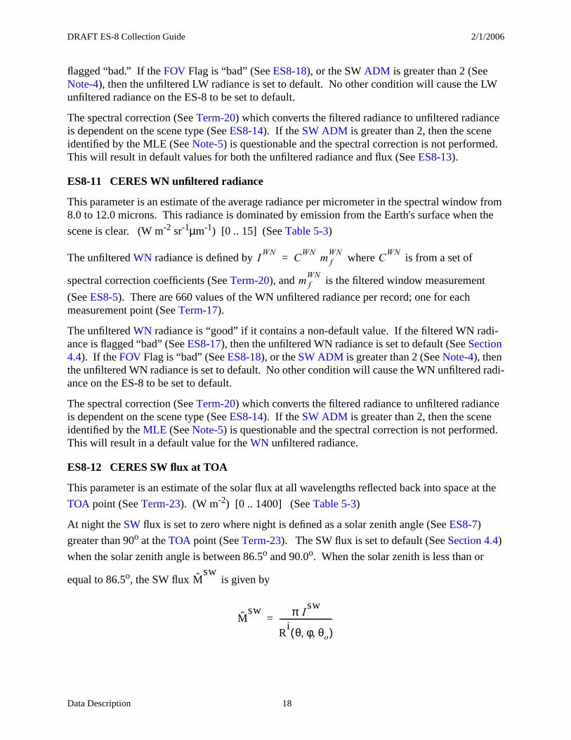
ES8-12 CERES SW flux at TOA
This parameter is an estimate of the solar flux at all wavelengths reflected back into space at the
TOA point (See Term-23). (W m-2) [0 .. 1400] (See Table 5-3)
At night the SW flux is set to zero where night is defined as a solar zenith angle (See ES8-7)
greater than 90o at the TOA point (See Term-23). The SW flux is set to default (See Section 4.4)
when the solar zenith angle is between 86.5o and 90.0o. When the solar zenith is less than or
equal to 86.5o, the SW flux is given by
IWN
CWN
m fWN
= CWN
m fWN
Msw
Msw π I
sw
Ri θ φ θo, ,( )
----------------------------=
DRAFT ES-8 Collection Guide 2/1/2006
Data Description 19
where is the shortwave radiance (See ES8-9), and R is the anisotropy (or ADM, See Note-4)
for the ith scene type (See ES8-14); and R is evaluated at the viewing zenith angle (See ES8-6),
relative azimuth angle (See ES8-8), and solar zenith angle (See ES8-7).
There are 660 values of the SW flux per record; one for each measurement point (See Term-17).
The SW flux is set to default if the SW radiance (See ES8-9) is default, or if the scene type (See ES8-14) is unknown, or if the instrument is operating in the rapid retrace mode (ES8-19). During
the day, where E=1365 d-2 and d=(ES8-V2). If albedo is greater
than 1.0 or less than 0.02, the SW flux is set to default. The SW flux is also set to default for
geometric conditions that lead to inaccurate flux estimates, or for , , and
.
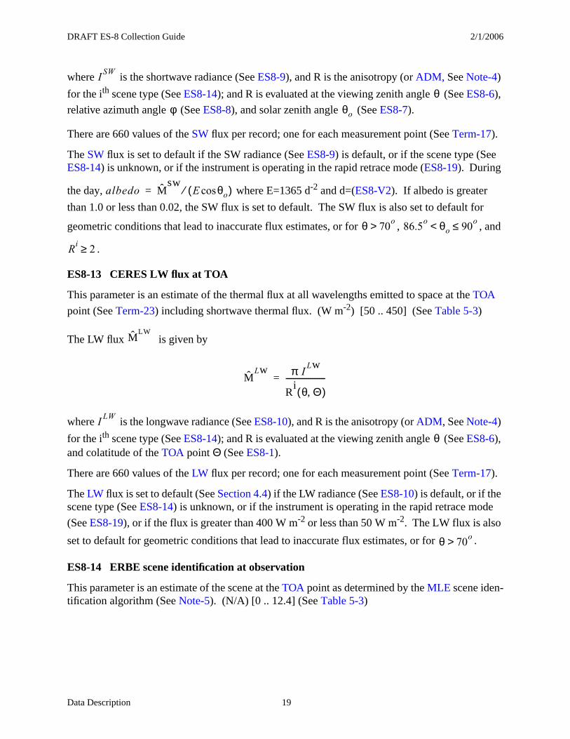
ES8-13 CERES LW flux at TOA
This parameter is an estimate of the thermal flux at all wavelengths emitted to space at the TOA
point (See Term-23) including shortwave thermal flux. (W m-2) [50 .. 450] (See Table 5-3)
The LW flux is given by
where is the longwave radiance (See ES8-10), and R is the anisotropy (or ADM, See Note-4)
for the ith scene type (See ES8-14); and R is evaluated at the viewing zenith angle (See ES8-6), and colatitude of the TOA point Θ (See ES8-1).
There are 660 values of the LW flux per record; one for each measurement point (See Term-17).
The LW flux is set to default (See Section 4.4) if the LW radiance (See ES8-10) is default, or if the scene type (See ES8-14) is unknown, or if the instrument is operating in the rapid retrace mode
(See ES8-19), or if the flux is greater than 400 W m-2 or less than 50 W m-2. The LW flux is also
set to default for geometric conditions that lead to inaccurate flux estimates, or for .
ES8-14 ERBE scene identification at observation
This parameter is an estimate of the scene at the TOA point as determined by the MLE scene iden-tification algorithm (See Note-5). (N/A) [0 .. 12.4] (See Table 5-3)
ISW
θφ θo
albedo Msw
E θocos( )⁄=
θ 70o> 86.5o θo 90o≤<
Ri 2≥
MLW
MLw π I
Lw
Ri θ Θ,( )
---------------------=
ILW
θ
θ 70o>
DRAFT ES-8 Collection Guide 2/1/2006
Data Description 20
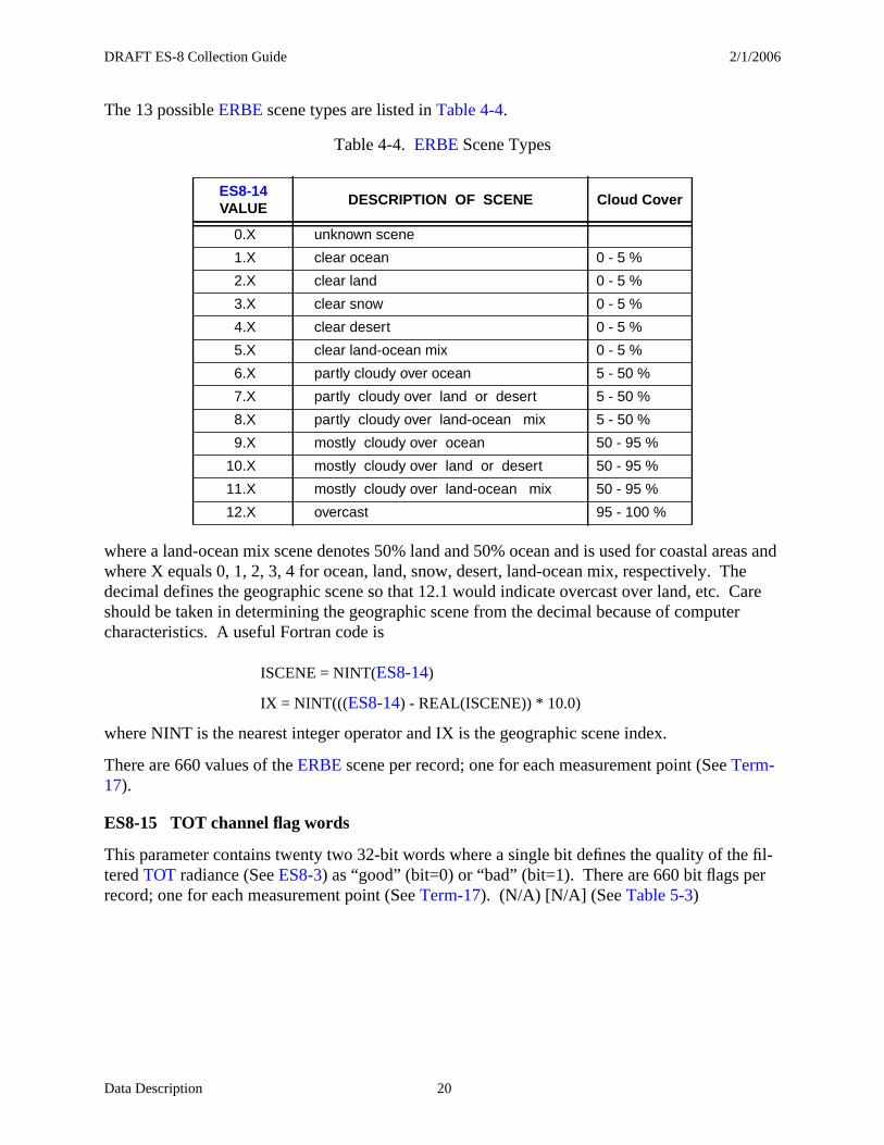
The 13 possible ERBE scene types are listed in Table 4-4.
where a land-ocean mix scene denotes 50% land and 50% ocean and is used for coastal areas and where X equals 0, 1, 2, 3, 4 for ocean, land, snow, desert, land-ocean mix, respectively. The decimal defines the geographic scene so that 12.1 would indicate overcast over land, etc. Care should be taken in determining the geographic scene from the decimal because of computer characteristics. A useful Fortran code is
ISCENE = NINT(ES8-14)
IX = NINT(((ES8-14) - REAL(ISCENE)) * 10.0)
where NINT is the nearest integer operator and IX is the geographic scene index.
There are 660 values of the ERBE scene per record; one for each measurement point (See Term-17).
ES8-15 TOT channel flag words
This parameter contains twenty two 32-bit words where a single bit defines the quality of the fil-tered TOT radiance (See ES8-3) as “good” (bit=0) or “bad” (bit=1). There are 660 bit flags per record; one for each measurement point (See Term-17). (N/A) [N/A] (See Table 5-3)
Table 4-4. ERBE Scene Types
ES8-14 VALUE
DESCRIPTION OF SCENE Cloud Cover
0.X unknown scene
1.X clear ocean 0 - 5 %
2.X clear land 0 - 5 %
3.X clear snow 0 - 5 %
4.X clear desert 0 - 5 %
5.X clear land-ocean mix 0 - 5 %
6.X partly cloudy over ocean 5 - 50 %
7.X partly cloudy over land or desert 5 - 50 %
8.X partly cloudy over land-ocean mix 5 - 50 %
9.X mostly cloudy over ocean 50 - 95 %
10.X mostly cloudy over land or desert 50 - 95 %
11.X mostly cloudy over land-ocean mix 50 - 95 %
12.X overcast 95 - 100 %
DRAFT ES-8 Collection Guide 2/1/2006
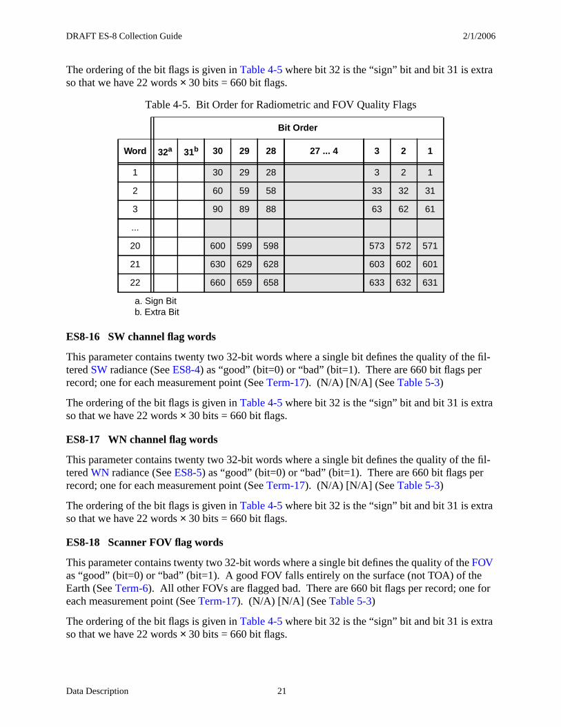
Data Description 21
The ordering of the bit flags is given in Table 4-5 where bit 32 is the “sign” bit and bit 31 is extra so that we have 22 words × 30 bits = 660 bit flags.
ES8-16 SW channel flag words
This parameter contains twenty two 32-bit words where a single bit defines the quality of the fil-tered SW radiance (See ES8-4) as “good” (bit=0) or “bad” (bit=1). There are 660 bit flags per record; one for each measurement point (See Term-17). (N/A) [N/A] (See Table 5-3)
The ordering of the bit flags is given in Table 4-5 where bit 32 is the “sign” bit and bit 31 is extra so that we have 22 words × 30 bits = 660 bit flags.
ES8-17 WN channel flag words
This parameter contains twenty two 32-bit words where a single bit defines the quality of the fil-tered WN radiance (See ES8-5) as “good” (bit=0) or “bad” (bit=1). There are 660 bit flags per record; one for each measurement point (See Term-17). (N/A) [N/A] (See Table 5-3)
The ordering of the bit flags is given in Table 4-5 where bit 32 is the “sign” bit and bit 31 is extra so that we have 22 words × 30 bits = 660 bit flags.
ES8-18 Scanner FOV flag words
This parameter contains twenty two 32-bit words where a single bit defines the quality of the FOV as “good” (bit=0) or “bad” (bit=1). A good FOV falls entirely on the surface (not TOA) of the Earth (See Term-6). All other FOVs are flagged bad. There are 660 bit flags per record; one for each measurement point (See Term-17). (N/A) [N/A] (See Table 5-3)
The ordering of the bit flags is given in Table 4-5 where bit 32 is the “sign” bit and bit 31 is extra so that we have 22 words × 30 bits = 660 bit flags.
Table 4-5. Bit Order for Radiometric and FOV Quality Flags
Bit Order
Word 32a
a. Sign Bit
31b
b. Extra Bit
30 29 28 27 ... 4 3 2 1
1 30 29 28 3 2 1
2 60 59 58 33 32 31
3 90 89 88 63 62 61
...
20 600 599 598 573 572 571
21 630 629 628 603 602 601
22 660 659 658 633 632 631
DRAFT ES-8 Collection Guide 2/1/2006
Data Description 22
ES8-19 Rapid retrace flag words
This parameter contains twenty two 32-bit words where a single bit defines the state of the scan rate as “not in rapid retrace” (bit=0) or “in rapid retrace” (bit=1). Rapid retrace (See Term-13) occurs during the short scan mode (See ES8-20). There are 660 rapid retrace bit flags per record; one for each measurement point (See Term-17). (N/A) [N/A] (See Table 5-3)
The ordering of the bit flags is given in Table 4-5 where bit 32 is the “sign” bit and bit 31 is extra so that we have 22 words × 30 bits = 660 bit flags.
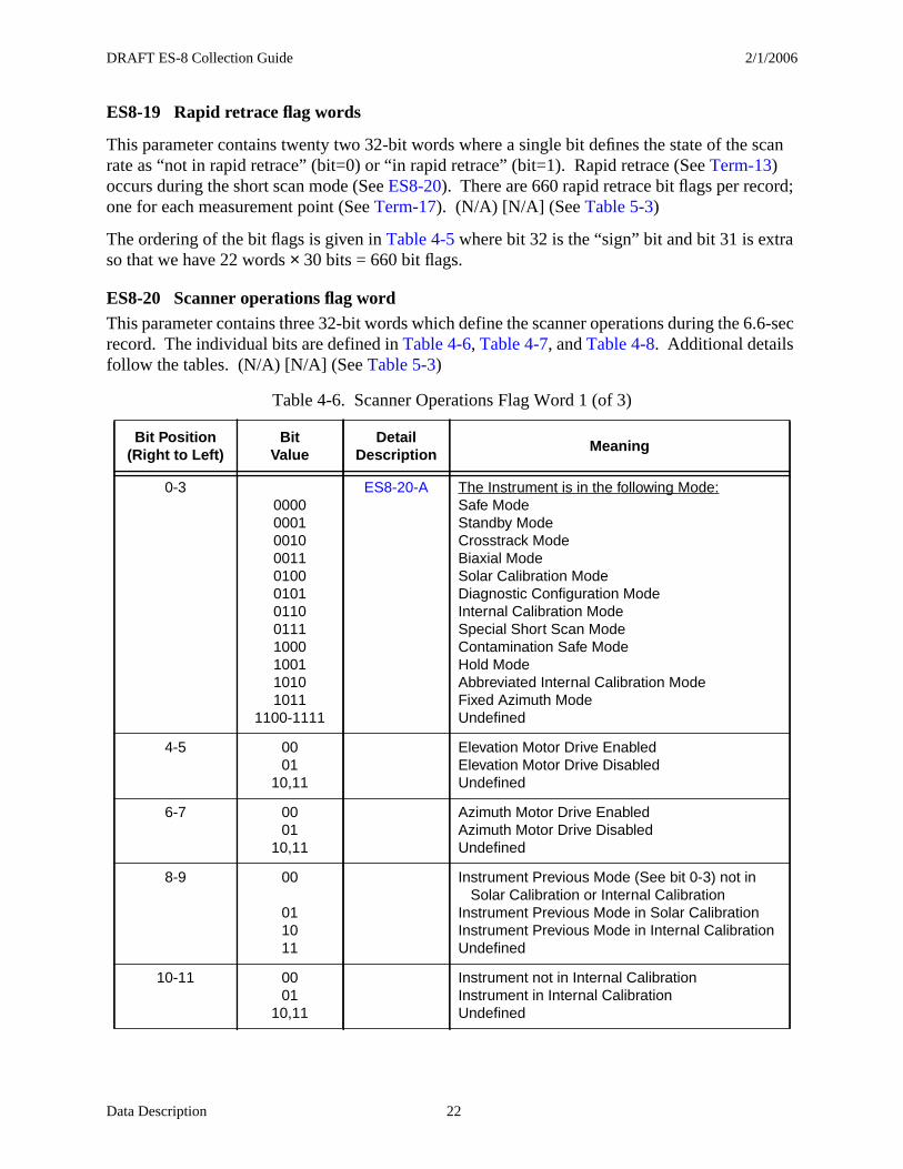
ES8-20 Scanner operations flag wordThis parameter contains three 32-bit words which define the scanner operations during the 6.6-sec record. The individual bits are defined in Table 4-6, Table 4-7, and Table 4-8. Additional details follow the tables. (N/A) [N/A] (See Table 5-3)
Table 4-6. Scanner Operations Flag Word 1 (of 3)
Bit Position(Right to Left)
BitValue
Detail Description
Meaning
0-3000000010010001101000101011001111000100110101011
1100-1111
ES8-20-A The Instrument is in the following Mode:Safe ModeStandby ModeCrosstrack ModeBiaxial ModeSolar Calibration ModeDiagnostic Configuration ModeInternal Calibration ModeSpecial Short Scan ModeContamination Safe ModeHold ModeAbbreviated Internal Calibration ModeFixed Azimuth ModeUndefined
4-5 0001
10,11
Elevation Motor Drive EnabledElevation Motor Drive DisabledUndefined
6-7 0001
10,11
Azimuth Motor Drive EnabledAzimuth Motor Drive DisabledUndefined
8-9 00
011011
Instrument Previous Mode (See bit 0-3) not in Solar Calibration or Internal CalibrationInstrument Previous Mode in Solar CalibrationInstrument Previous Mode in Internal CalibrationUndefined
10-11 0001
10,11
Instrument not in Internal CalibrationInstrument in Internal CalibrationUndefined
DRAFT ES-8 Collection Guide 2/1/2006
Data Description 23
See detail descriptions after Table 4-8.
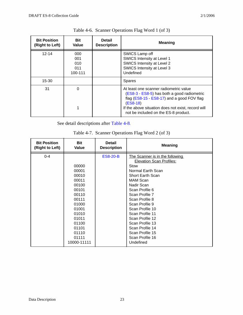
12-14 000001010011
100-111
SWICS Lamp offSWICS Intensity at Level 1SWICS Intensity at Level 2SWICS Intensity at Level 3Undefined
15-30 Spares
31 0
1
At least one scanner radiometric value (ES8-3 - ES8-5) has both a good radiometric flag (ES8-15 - ES8-17) and a good FOV flag (ES8-18)If the above situation does not exist, record will not be included on the ES-8 product.
Table 4-7. Scanner Operations Flag Word 2 (of 3)
Bit Position(Right to Left)
BitValue
Detail Description
Meaning
0-4
00000000010001000011001000010100110001110100001001010100101101100011010111001111
10000-11111
ES8-20-B The Scanner is in the following Elevation Scan Profiles:StowNormal Earth ScanShort Earth ScanMAM ScanNadir ScanScan Profile 6Scan Profile 7Scan Profile 8Scan Profile 9Scan Profile 10Scan Profile 11Scan Profile 12Scan Profile 13Scan Profile 14Scan Profile 15Scan Profile 16Undefined
Table 4-6. Scanner Operations Flag Word 1 (of 3)
Bit Position(Right to Left)
BitValue
Detail Description
Meaning
DRAFT ES-8 Collection Guide 2/1/2006
Data Description 24
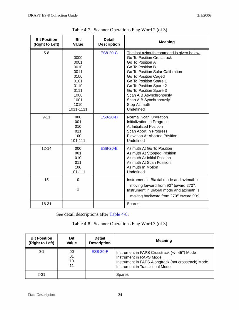
See detail descriptions after Table 4-8.
5-800000001001000110100010101100111100010011010
1011-1111
ES8-20-C The last azimuth command is given below:Go To Position CrosstrackGo To Position AGo To Position BGo To Position Solar CalibrationGo To Position CagedGo To Position Spare 1Go To Position Spare 2Go To Position Spare 3Scan A B AsynchronouslyScan A B SynchronouslyStop AzimuthUndefined
9-11 000001010011100
101-111
ES8-20-D Normal Scan OperationInitialization In ProgressAt Initialized PositionScan Abort In ProgressElevation At Aborted PositionUndefined
12-14 000001010011100
101-111
ES8-20-E Azimuth At Go To PositionAzimuth At Stopped PositionAzimuth At Initial PositionAzimuth At Scan PositionAzimuth In MotionUndefined
15 0
1
Instrument in Biaxial mode and azimuth is
moving forward from 90o toward 270o.Instrument in Biaxial mode and azimuth is
moving backward from 270o toward 90o.
16-31 Spares
Table 4-8. Scanner Operations Flag Word 3 (of 3)
Bit Position(Right to Left)
BitValue
Detail Description
Meaning
0-1 00011011
ES8-20-F Instrument in FAPS Crosstrack (+/- 45o) ModeInstrument in RAPS ModeInstrument in FAPS Alongtrack (not crosstrack) ModeInstrument in Transitional Mode
2-31 Spares
Table 4-7. Scanner Operations Flag Word 2 (of 3)
Bit Position(Right to Left)
BitValue
Detail Description
Meaning
DRAFT ES-8 Collection Guide 2/1/2006
Data Description 25
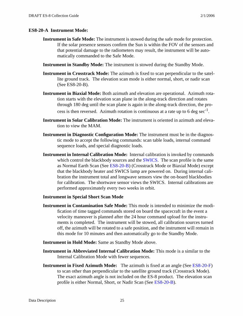
ES8-20-A Instrument Mode:
Instrument in Safe Mode: The instrument is stowed during the safe mode for protection. If the solar presence sensors confirm the Sun is within the FOV of the sensors and that potential damage to the radiometers may result, the instrument will be auto-matically commanded to the Safe Mode.
Instrument in Standby Mode: The instrument is stowed during the Standby Mode.
Instrument in Crosstrack Mode: The azimuth is fixed to scan perpendicular to the satel-lite ground track. The elevation scan mode is either normal, short, or nadir scan (See ES8-20-B).
Instrument in Biaxial Mode: Both azimuth and elevation are operational. Azimuth rota-tion starts with the elevation scan plane in the along-track direction and rotates through 180 deg until the scan plane is again in the along-track direction, the pro-
cess is then reversed. Azimuth rotation is continuous at a rate up to 6 deg sec-1.
Instrument in Solar Calibration Mode: The instrument is oriented in azimuth and eleva-tion to view the MAM.
Instrument in Diagnostic Configuration Mode: The instrument must be in the diagnos-tic mode to accept the following commands: scan table loads, internal command sequence loads, and special diagnostic loads.
Instrument in Internal Calibration Mode: Internal calibration is invoked by commands which control the blackbody sources and the SWICS. The scan profile is the same as Normal Earth Scan (See ES8-20-B) (Crosstrack Mode or Biaxial Mode) except that the blackbody heater and SWICS lamp are powered on. During internal cali-bration the instrument total and longwave sensors view the on-board blackbodies for calibration. The shortwave sensor views the SWICS. Internal calibrations are performed approximately every two weeks in orbit.
Instrument in Special Short Scan Mode
Instrument in Contamination Safe Mode: This mode is intended to minimize the modi-fication of time tagged commands stored on board the spacecraft in the event a velocity maneuver is planned after the 24 hour command upload for the instru-ments is completed. The instrument will be stowed, all calibration sources turned off, the azimuth will be rotated to a safe position, and the instrument will remain in this mode for 10 minutes and then automatically go to the Standby Mode.
Instrument in Hold Mode: Same as Standby Mode above.
Instrument in Abbreviated Internal Calibration Mode: This mode is a similar to the Internal Calibration Mode with fewer sequences.
Instrument in Fixed Azimuth Mode: The azimuth is fixed at an angle (See ES8-20-F) to scan other than perpendicular to the satellite ground track (Crosstrack Mode). The exact azimuth angle is not included on the ES-8 product. The elevation scan profile is either Normal, Short, or Nadir Scan (See ES8-20-B).
DRAFT ES-8 Collection Guide 2/1/2006
Data Description 26
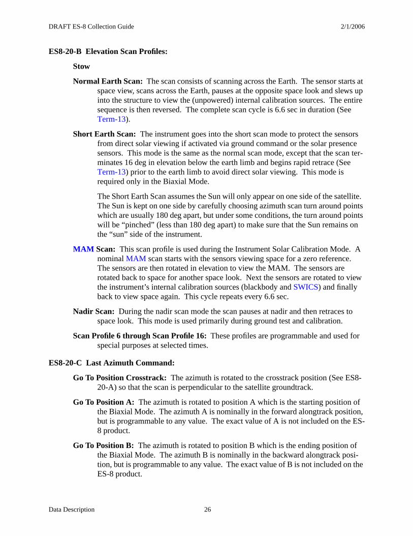
ES8-20-B Elevation Scan Profiles:
Stow
Normal Earth Scan: The scan consists of scanning across the Earth. The sensor starts at space view, scans across the Earth, pauses at the opposite space look and slews up into the structure to view the (unpowered) internal calibration sources. The entire sequence is then reversed. The complete scan cycle is 6.6 sec in duration (See Term-13).
Short Earth Scan: The instrument goes into the short scan mode to protect the sensors from direct solar viewing if activated via ground command or the solar presence sensors. This mode is the same as the normal scan mode, except that the scan ter-minates 16 deg in elevation below the earth limb and begins rapid retrace (See Term-13) prior to the earth limb to avoid direct solar viewing. This mode is required only in the Biaxial Mode.
The Short Earth Scan assumes the Sun will only appear on one side of the satellite. The Sun is kept on one side by carefully choosing azimuth scan turn around points which are usually 180 deg apart, but under some conditions, the turn around points will be “pinched” (less than 180 deg apart) to make sure that the Sun remains on the “sun” side of the instrument.
MAM Scan: This scan profile is used during the Instrument Solar Calibration Mode. A nominal MAM scan starts with the sensors viewing space for a zero reference. The sensors are then rotated in elevation to view the MAM. The sensors are rotated back to space for another space look. Next the sensors are rotated to view the instrument’s internal calibration sources (blackbody and SWICS) and finally back to view space again. This cycle repeats every 6.6 sec.
Nadir Scan: During the nadir scan mode the scan pauses at nadir and then retraces to space look. This mode is used primarily during ground test and calibration.
Scan Profile 6 through Scan Profile 16: These profiles are programmable and used for special purposes at selected times.
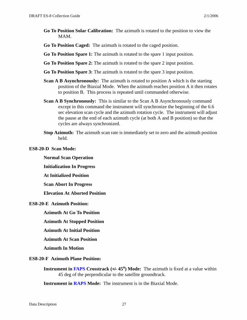
ES8-20-C Last Azimuth Command:
Go To Position Crosstrack: The azimuth is rotated to the crosstrack position (See ES8-20-A) so that the scan is perpendicular to the satellite groundtrack.
Go To Position A: The azimuth is rotated to position A which is the starting position of the Biaxial Mode. The azimuth A is nominally in the forward alongtrack position, but is programmable to any value. The exact value of A is not included on the ES-8 product.
Go To Position B: The azimuth is rotated to position B which is the ending position of the Biaxial Mode. The azimuth B is nominally in the backward alongtrack posi-tion, but is programmable to any value. The exact value of B is not included on the ES-8 product.
DRAFT ES-8 Collection Guide 2/1/2006
Data Description 27
Go To Position Solar Calibration: The azimuth is rotated to the position to view the MAM.
Go To Position Caged: The azimuth is rotated to the caged position.
Go To Position Spare 1: The azimuth is rotated to the spare 1 input position.
Go To Position Spare 2: The azimuth is rotated to the spare 2 input position.
Go To Position Spare 3: The azimuth is rotated to the spare 3 input position.
Scan A B Asynchronously: The azimuth is rotated to position A which is the starting position of the Biaxial Mode. When the azimuth reaches position A it then rotates to position B. This process is repeated until commanded otherwise.
Scan A B Synchronously: This is similar to the Scan A B Asynchronously command except in this command the instrument will synchronize the beginning of the 6.6 sec elevation scan cycle and the azimuth rotation cycle. The instrument will adjust the pause at the end of each azimuth cycle (at both A and B position) so that the cycles are always synchronized.
Stop Azimuth: The azimuth scan rate is immediately set to zero and the azimuth position held.
ES8-20-D Scan Mode:
Normal Scan Operation
Initialization In Progress
At Initialized Position
Scan Abort In Progress
Elevation At Aborted Position
ES8-20-E Azimuth Position:
Azimuth At Go To Position
Azimuth At Stopped Position
Azimuth At Initial Position
Azimuth At Scan Position
Azimuth In Motion
ES8-20-F Azimuth Plane Position:
Instrument in FAPS Crosstrack (+/- 45o) Mode: The azimuth is fixed at a value within 45 deg of the perpendicular to the satellite groundtrack.
Instrument in RAPS Mode: The instrument is in the Biaxial Mode.
DRAFT ES-8 Collection Guide 2/1/2006
Data Description 28
Instrument in FAPS Alongtrack (not crosstrack) Mode: The azimuth is fixed at a value greater than 45 deg from the perpendicular to the satellite groundtrack.
Instrument in Transitional Mode: The azimuth is in transition between modes.
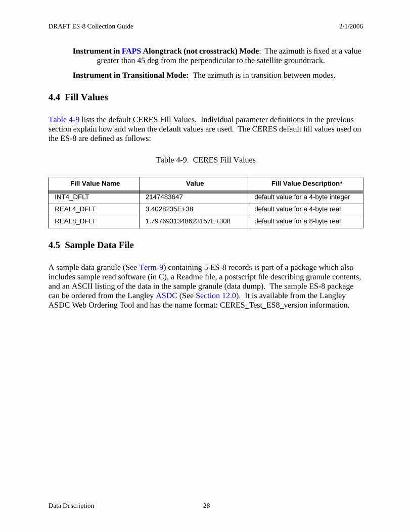
4.4 Fill Values
Table 4-9 lists the default CERES Fill Values. Individual parameter definitions in the previous section explain how and when the default values are used. The CERES default fill values used on the ES-8 are defined as follows:
Table 4-9. CERES Fill Values
4.5 Sample Data File
A sample data granule (See Term-9) containing 5 ES-8 records is part of a package which also includes sample read software (in C), a Readme file, a postscript file describing granule contents, and an ASCII listing of the data in the sample granule (data dump). The sample ES-8 package can be ordered from the Langley ASDC (See Section 12.0). It is available from the Langley ASDC Web Ordering Tool and has the name format: CERES_Test_ES8_version information.
Fill Value Name Value Fill Value Description*
INT4_DFLT 2147483647 default value for a 4-byte integer
REAL4_DFLT 3.4028235E+38 default value for a 4-byte real
REAL8_DFLT 1.7976931348623157E+308 default value for a 8-byte real
DRAFT ES-8 Collection Guide 2/1/2006
Data Organization 29
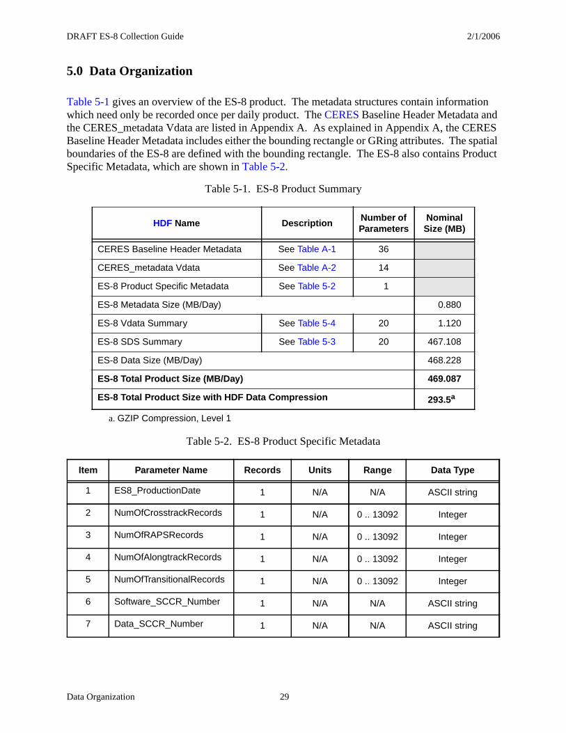
5.0 Data Organization
Table 5-1 gives an overview of the ES-8 product. The metadata structures contain information which need only be recorded once per daily product. The CERES Baseline Header Metadata and the CERES_metadata Vdata are listed in Appendix A. As explained in Appendix A, the CERES Baseline Header Metadata includes either the bounding rectangle or GRing attributes. The spatial boundaries of the ES-8 are defined with the bounding rectangle. The ES-8 also contains Product Specific Metadata, which are shown in Table 5-2.
Table 5-1. ES-8 Product Summary
HDF Name DescriptionNumber of Parameters
Nominal Size (MB)
CERES Baseline Header Metadata See Table A-1 36
CERES_metadata Vdata See Table A-2 14
ES-8 Product Specific Metadata See Table 5-2 1
ES-8 Metadata Size (MB/Day) 0.880
ES-8 Vdata Summary See Table 5-4 20 1.120
ES-8 SDS Summary See Table 5-3 20 467.108
ES-8 Data Size (MB/Day) 468.228
ES-8 Total Product Size (MB/Day) 469.087
ES-8 Total Product Size with HDF Data Compression 293.5a
a. GZIP Compression, Level 1
Table 5-2. ES-8 Product Specific Metadata
Item Parameter Name Records Units Range Data Type
1 ES8_ProductionDate 1 N/A N/A ASCII string
2 NumOfCrosstrackRecords 1 N/A 0 .. 13092 Integer
3 NumOfRAPSRecords 1 N/A 0 .. 13092 Integer
4 NumOfAlongtrackRecords 1 N/A 0 .. 13092 Integer
5 NumOfTransitionalRecords 1 N/A 0 .. 13092 Integer
6 Software_SCCR_Number 1 N/A N/A ASCII string
7 Data_SCCR_Number 1 N/A N/A ASCII string
DRAFT ES-8 Collection Guide 2/1/2006
Data Organization 30
5.1 Data Granularity
All ES-8 HDF data granules consist of no more than 24 hours of data from one CERES instrument.
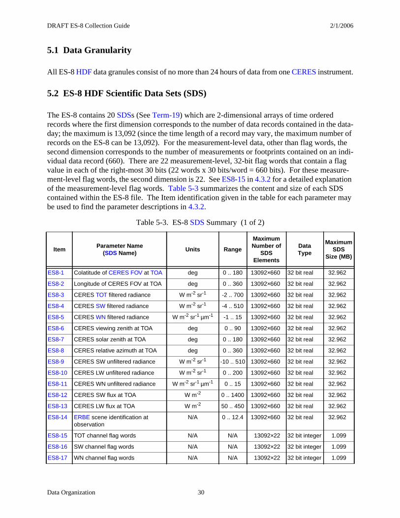
5.2 ES-8 HDF Scientific Data Sets (SDS)
The ES-8 contains 20 SDSs (See Term-19) which are 2-dimensional arrays of time ordered records where the first dimension corresponds to the number of data records contained in the data-day; the maximum is 13,092 (since the time length of a record may vary, the maximum number of records on the ES-8 can be 13,092). For the measurement-level data, other than flag words, the second dimension corresponds to the number of measurements or footprints contained on an indi-vidual data record (660). There are 22 measurement-level, 32-bit flag words that contain a flag value in each of the right-most 30 bits (22 words x 30 bits/word = 660 bits). For these measure-ment-level flag words, the second dimension is 22. See ES8-15 in 4.3.2 for a detailed explanation of the measurement-level flag words. Table 5-3 summarizes the content and size of each SDS contained within the ES-8 file. The Item identification given in the table for each parameter may be used to find the parameter descriptions in 4.3.2.
Table 5-3. ES-8 SDS Summary (1 of 2)
ItemParameter Name
(SDS Name)Units Range
MaximumNumber of
SDSElements
DataType
MaximumSDS
Size (MB)
ES8-1 Colatitude of CERES FOV at TOA deg 0 .. 180 13092×660 32 bit real 32.962
ES8-2 Longitude of CERES FOV at TOA deg 0 .. 360 13092×660 32 bit real 32.962
ES8-3 CERES TOT filtered radiance W m-2 sr-1 -2 .. 700 13092×660 32 bit real 32.962
ES8-4 CERES SW filtered radiance W m-2 sr-1 -4 .. 510 13092×660 32 bit real 32.962
ES8-5 CERES WN filtered radiance W m-2 sr-1 µm-1 -1 .. 15 13092×660 32 bit real 32.962
ES8-6 CERES viewing zenith at TOA deg 0 .. 90 13092×660 32 bit real 32.962
ES8-7 CERES solar zenith at TOA deg 0 .. 180 13092×660 32 bit real 32.962
ES8-8 CERES relative azimuth at TOA deg 0 .. 360 13092×660 32 bit real 32.962
ES8-9 CERES SW unfiltered radiance W m-2 sr-1 -10 .. 510 13092×660 32 bit real 32.962
ES8-10 CERES LW unfiltered radiance W m-2 sr-1 0 .. 200 13092×660 32 bit real 32.962
ES8-11 CERES WN unfiltered radiance W m-2 sr-1 µm-1 0 .. 15 13092×660 32 bit real 32.962
ES8-12 CERES SW flux at TOA W m-2 0 .. 1400 13092×660 32 bit real 32.962
ES8-13 CERES LW flux at TOA W m-2 50 .. 450 13092×660 32 bit real 32.962
ES8-14 ERBE scene identification at observation
N/A 0 .. 12.4 13092×660 32 bit real 32.962
ES8-15 TOT channel flag words N/A N/A 13092×22 32 bit integer 1.099
ES8-16 SW channel flag words N/A N/A 13092×22 32 bit integer 1.099
ES8-17 WN channel flag words N/A N/A 13092×22 32 bit integer 1.099
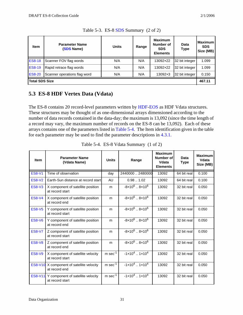
DRAFT ES-8 Collection Guide 2/1/2006
Data Organization 31
5.3 ES-8 HDF Vertex Data (Vdata)
The ES-8 contains 20 record-level parameters written by HDF-EOS as HDF Vdata structures. These structures may be thought of as one-dimensional arrays dimensioned according to the number of data records contained in the data-day; the maximum is 13,092 (since the time length of a record may vary, the maximum number of records on the ES-8 can be 13,092). Each of these arrays contains one of the parameters listed in Table 5-4. The Item identification given in the table for each parameter may be used to find the parameter descriptions in 4.3.1.
ES8-18 Scanner FOV flag words N/A N/A 13092×22 32 bit integer 1.099
ES8-19 Rapid retrace flag words N/A N/A 13092×22 32 bit integer 1.099
ES8-20 Scanner operations flag word N/A N/A 13092×3 32 bit integer 0.150
Total SDS Size 467.11
Table 5-4. ES-8 Vdata Summary (1 of 2)
ItemParameter Name
(Vdata Name)Units Range
MaximumNumber of
VdataElements
DataType
MaximumVdata
Size (MB)
ES8-V1 Time of observation day 2440000 .. 2480000 13092 64 bit real 0.100
ES8-V2 Earth-Sun distance at record start AU 0.98 .. 1.02 13092 64 bit real 0.100
ES8-V3 X component of satellite position at record start
m -8×10⁶ .. 8×10⁶ 13092 32 bit real 0.050
ES8-V4 X component of satellite position at record end
m -8×10⁶ .. 8×10⁶ 13092 32 bit real 0.050
ES8-V5 Y component of satellite position at record start
m -8×10⁶ .. 8×10⁶ 13092 32 bit real 0.050
ES8-V6 Y component of satellite position at record end
m -8×10⁶ .. 8×10⁶ 13092 32 bit real 0.050
ES8-V7 Z component of satellite position at record start
m -8×10⁶ .. 8×10⁶ 13092 32 bit real 0.050
ES8-V8 Z component of satellite position at record end
m -8×10⁶ .. 8×10⁶ 13092 32 bit real 0.050
ES8-V9 X component of satellite velocity at record start
m sec-1 -1×10⁴ .. 1×10⁴ 13092 32 bit real 0.050
ES8-V10 X component of satellite velocity at record end
m sec-1 -1×10⁴ .. 1×10⁴ 13092 32 bit real 0.050
ES8-V11 Y component of satellite velocity at record start
m sec-1 -1×10⁴ .. 1×10⁴ 13092 32 bit real 0.050
Table 5-3. ES-8 SDS Summary (2 of 2)
ItemParameter Name
(SDS Name)Units Range
MaximumNumber of
SDSElements
DataType
MaximumSDS
Size (MB)
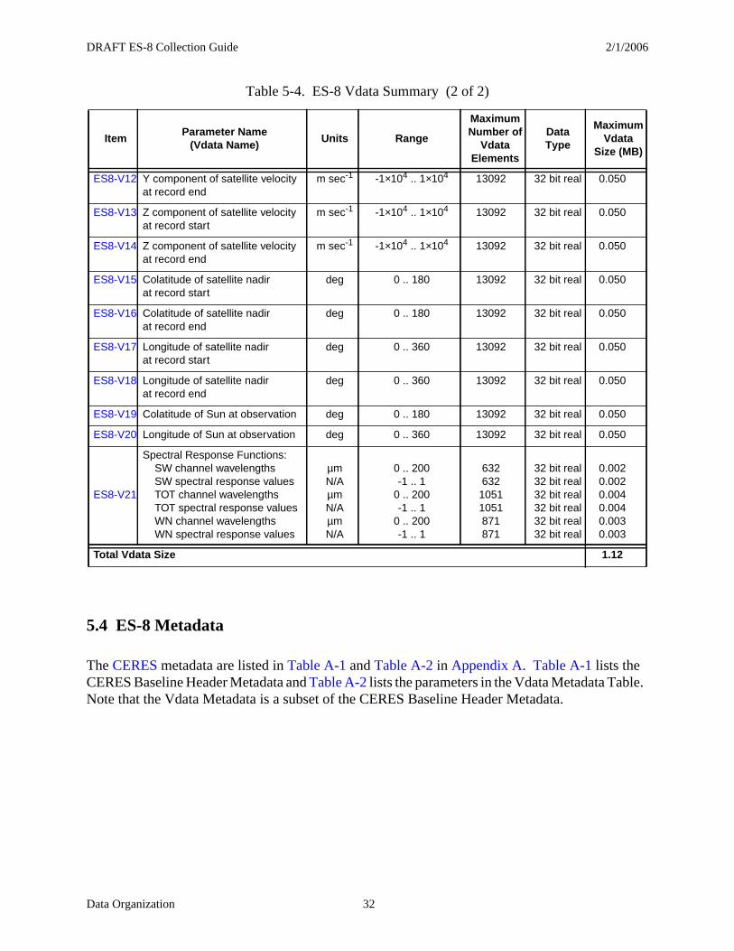
DRAFT ES-8 Collection Guide 2/1/2006
Data Organization 32
5.4 ES-8 Metadata
The CERES metadata are listed in Table A-1 and Table A-2 in Appendix A. Table A-1 lists the CERES Baseline Header Metadata and Table A-2 lists the parameters in the Vdata Metadata Table. Note that the Vdata Metadata is a subset of the CERES Baseline Header Metadata.
ES8-V12 Y component of satellite velocity at record end
m sec-1 -1×10⁴ .. 1×10⁴ 13092 32 bit real 0.050
ES8-V13 Z component of satellite velocity at record start
m sec-1 -1×10⁴ .. 1×10⁴ 13092 32 bit real 0.050
ES8-V14 Z component of satellite velocity at record end
m sec-1 -1×10⁴ .. 1×10⁴ 13092 32 bit real 0.050
ES8-V15 Colatitude of satellite nadirat record start
deg 0 .. 180 13092 32 bit real 0.050
ES8-V16 Colatitude of satellite nadirat record end
deg 0 .. 180 13092 32 bit real 0.050
ES8-V17 Longitude of satellite nadirat record start
deg 0 .. 360 13092 32 bit real 0.050
ES8-V18 Longitude of satellite nadirat record end
deg 0 .. 360 13092 32 bit real 0.050
ES8-V19 Colatitude of Sun at observation deg 0 .. 180 13092 32 bit real 0.050
ES8-V20 Longitude of Sun at observation deg 0 .. 360 13092 32 bit real 0.050
ES8-V21
Spectral Response Functions: SW channel wavelengths SW spectral response values TOT channel wavelengths TOT spectral response values WN channel wavelengths WN spectral response values
µmN/AµmN/AµmN/A
0 .. 200-1 .. 1
0 .. 200-1 .. 1
0 .. 200-1 .. 1
63263210511051871871
32 bit real32 bit real32 bit real32 bit real32 bit real32 bit real
0.0020.0020.0040.0040.0030.003
Total Vdata Size 1.12
Table 5-4. ES-8 Vdata Summary (2 of 2)
ItemParameter Name
(Vdata Name)Units Range
MaximumNumber of
VdataElements
DataType
MaximumVdata
Size (MB)
DRAFT ES-8 Collection Guide 2/1/2006
Theory of Measurements and Data Manipulations 33
6.0 Theory of Measurements and Data Manipulations
6.1 Theory of Measurements
See CERES ATBD Subsystem 2.0 (Reference 5).
6.2 Data Processing Sequence
The ERBE-like Inversion Subsystem (2.0) converts filtered radiometric measurements in engineering units received from the Instrument Subsystem (1.0) to instantaneous flux estimates at the TOA. This inversion process is dependent on several factors, including Earth surface features, the extent of cloudiness, and the relative geometry of the spacecraft, the sun, and the measurement FOV. Each radiometric measurement is spectrally corrected to give an unfiltered measurement. The observed scene is determined by a scene identification algorithm based on these unfiltered measurements, using angular distribution models and statistics provided by the CERES Science Team. Estimates of the radiant flux at the TOA are computed based on scene information, geometrical considerations, and the unfiltered measurements.
For detailed information see the ERBE-like Software Requirements Document (Subsystem 2.0) (Reference 6).
6.3 Special Corrections/Adjustments
Algorithms not discussed in the ATBD are discussed in this section.
DRAFT ES-8 Collection Guide 2/1/2006
Errors 34
7.0 Errors
See the Data Quality Summary {URL=http://eosweb.larc.nasa.gov/project/ceres/ES8/disclaimer_CER_ES8.html}.
7.1 Quality Assessment
QA activities are performed at the Science Computing Facility by the Data Management Team. Processing reports containing statistics and processing results are examined for anomalies. If the reports show anomalies, data visualization tools are used to examine those products in greater detail to begin the anomaly investigation. (See the QA flag description for this product.)
7.2 Data Validation by Source
See Subsystem 2.0 Validation Document (Reference 7) for details on the data validation plan.
DRAFT ES-8 Collection Guide 2/1/2006
Notes 35
8.0 Notes
Notes are given to expand on subjects that will help in the use and understanding of the ES-8 product. These notes are generally characterized by more details and longer length than other definitions (See Section 4.3).
Note-1 Conversion of Julian Date to Calendar Date
The Julian Date is a time system that has been adopted by astronomers and is used in many scientific experiments. The Julian Date or Julian Day is the number of mean solar days since 1200 hours (GMT/UT/UTC/Zulu) on Monday, 24 November 4714 BCE, based on the current Gregorian calendar, or more precisely, the Gregorian Proleptic calendar. In other words, Julian day number 0 (zero) was Monday, 24 November 4714 BCE, 1200 hours (noon). A new Julian day starts when the mean Sun at noon crosses the Greenwich meridian. This differs from UT or Greenwich Mean Solar Time by 12 hours since UT changes day at Greenwich midnight. Table 8-1 below provides Julian day numbers which relate UT to Julian date.
Important facts related to the Gregorian calendar are:
a) There is no year zero; year -1 is immediately followed by year 1.
b) A leap year is any year which is divisible by 4, except for those centesimal years (years divisible by 100) which must also be divisible by 400 to be considered a leap year.
c) A leap year has 366 days, with the month of February containing 29 days.
d) Year -1 is defined as a leap year, thus being also defined as containing 366 days, and being divisible by 4, 100, and 400.
Information on history, calendars, and Julian day numbers can be found in Blackadar’s “A Computer Almanac” (See Reference 8) and on the WWW (See Reference 9).
The Julian day whole number is followed by the fraction of the day that has elapsed since the preceding noon (1200 hours UTC). The Julian Date JDATE can be represented as:
JDATE = JDay + JFractwhere:
JDay = the integer Julian Day number andJFract = the “fractional” Julian day (0 to 0.99...9)
(e.g. 245_0814.0 = 1200 or noon, 31 December, 1997 UT)
When the fractional part of the combined Julian date is .0, it is noon or 1200 hours GMT and when the fraction part is .5, then it is midnight or 0000 hours GMT.
The calculation of GMT (YYYYMMDD-HH:MM:SS.SSS) from Julian date (JDATE) is performed using the following process.
1. The YYYYMMDD can be determined using Table 8-1 to find the year and the beginning of the month whose Julian Day occurs before the JDay integer value.
DRAFT ES-8 Collection Guide 2/1/2006
Notes 36
2. Calculate the number of days past the 0.5 day of the month via Table 8-1 which provides Julian day numbers which relate UT to Julian date.
The GMT is determined by first computing the number of seconds in the day since midnight:if JFract > 0.5,then Seconds = 86400.0 * (JFract-0.5)if JFract <= 0.5, then Seconds = 86400.0 * (JFract+0.5)
Then compute HH, MM, and SS where:HH = Int(Seconds/3600)MM = Int(Seconds-(HH*3600.0)/60)SS = Seconds-(HH*60.0 + MM)*60.0
As an example, if JD = 244_5733.5833, then the GMT date is computed using Table 8-1 by finding the closest beginning monthly calendar noon date, which is Feb 0.5, 1984 (UT).
(Feb 0.5) Jday244_5731 < 244_5733.5833
JD = 244_5733.5833 is 2.5833 days past Feb 0.5, 1984 UT (i.e., past 1984 Jan 31d 12h 0m 0s)
where 1984 Jan 31d 12h 0m 0s = (244_5733-244_5731).
Beginning with the whole days portion of 2.5833 (i.e., 2), the GMT Date is
1984 Jan 31d 12h 0m 0s + 2 = 1984 Feb 2d 12h 0m 0s.
Next, since JFract (0.5833) is > 0.5, 12h is added to the GMT Date, yielding:
1984 Feb 2d 12h 0m 0s + 12h 0m 0s = 1984 Feb 3d 0h 0m 0s.
Finally, to get the GMT time and since JFract (0.5833) is > 0.5, the number of seconds = 86400 *(0.5833 -0.5) = 7197.12 yielding:
HH = 7197.12 / 3600 = 01.9992 = 01h
MM = 7197.12 - ((1*3600) / 60) = 59.952 = 59m
SS = 7197.12 - ((1*60) + 59)*60) = 57.12s
Therefore, the GMT Date corresponding to the Julian Date 244_5733.5833 =
1984 Feb 3d 1h 59m 57.12s, which is UT = 1984 Jan 31d 12h 0m 0s + 2.5833 days.
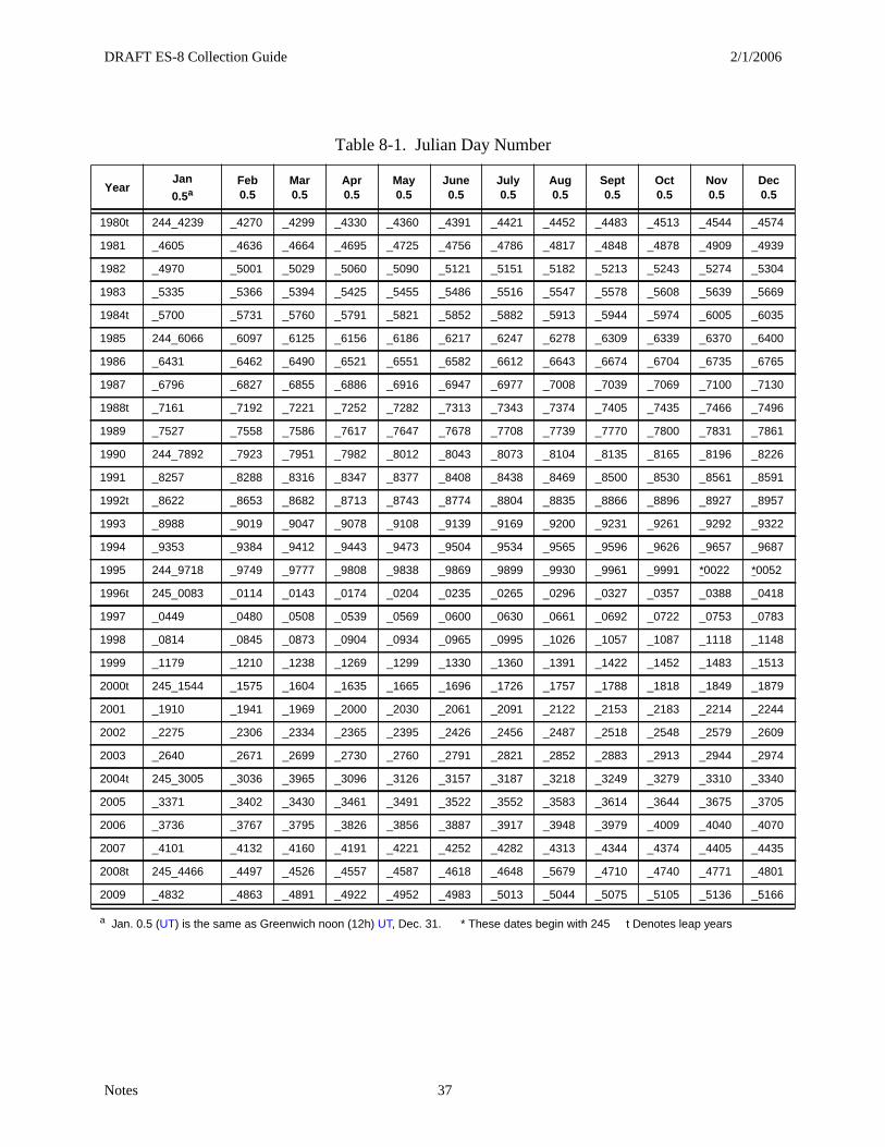
DRAFT ES-8 Collection Guide 2/1/2006
Notes 37
Table 8-1. Julian Day Number
YearJan
0.5aFeb 0.5
Mar 0.5
Apr 0.5
May 0.5
June 0.5
July 0.5
Aug 0.5
Sept 0.5
Oct 0.5
Nov 0.5
Dec 0.5
1980t 244_4239 _4270 _4299 _4330 _4360 _4391 _4421 _4452 _4483 _4513 _4544 _4574
1981 _4605 _4636 _4664 _4695 _4725 _4756 _4786 _4817 _4848 _4878 _4909 _4939
1982 _4970 _5001 _5029 _5060 _5090 _5121 _5151 _5182 _5213 _5243 _5274 _5304
1983 _5335 _5366 _5394 _5425 _5455 _5486 _5516 _5547 _5578 _5608 _5639 _5669
1984t _5700 _5731 _5760 _5791 _5821 _5852 _5882 _5913 _5944 _5974 _6005 _6035
1985 244_6066 _6097 _6125 _6156 _6186 _6217 _6247 _6278 _6309 _6339 _6370 _6400
1986 _6431 _6462 _6490 _6521 _6551 _6582 _6612 _6643 _6674 _6704 _6735 _6765
1987 _6796 _6827 _6855 _6886 _6916 _6947 _6977 _7008 _7039 _7069 _7100 _7130
1988t _7161 _7192 _7221 _7252 _7282 _7313 _7343 _7374 _7405 _7435 _7466 _7496
1989 _7527 _7558 _7586 _7617 _7647 _7678 _7708 _7739 _7770 _7800 _7831 _7861
1990 244_7892 _7923 _7951 _7982 _8012 _8043 _8073 _8104 _8135 _8165 _8196 _8226
1991 _8257 _8288 _8316 _8347 _8377 _8408 _8438 _8469 _8500 _8530 _8561 _8591
1992t _8622 _8653 _8682 _8713 _8743 _8774 _8804 _8835 _8866 _8896 _8927 _8957
1993 _8988 _9019 _9047 _9078 _9108 _9139 _9169 _9200 _9231 _9261 _9292 _9322
1994 _9353 _9384 _9412 _9443 _9473 _9504 _9534 _9565 _9596 _9626 _9657 _9687
1995 244_9718 _9749 _9777 _9808 _9838 _9869 _9899 _9930 _9961 _9991 *0022 *0052
1996t 245_0083 _0114 _0143 _0174 _0204 _0235 _0265 _0296 _0327 _0357 _0388 _0418
1997 _0449 _0480 _0508 _0539 _0569 _0600 _0630 _0661 _0692 _0722 _0753 _0783
1998 _0814 _0845 _0873 _0904 _0934 _0965 _0995 _1026 _1057 _1087 _1118 _1148
1999 _1179 _1210 _1238 _1269 _1299 _1330 _1360 _1391 _1422 _1452 _1483 _1513
2000t 245_1544 _1575 _1604 _1635 _1665 _1696 _1726 _1757 _1788 _1818 _1849 _1879
2001 _1910 _1941 _1969 _2000 _2030 _2061 _2091 _2122 _2153 _2183 _2214 _2244
2002 _2275 _2306 _2334 _2365 _2395 _2426 _2456 _2487 _2518 _2548 _2579 _2609
2003 _2640 _2671 _2699 _2730 _2760 _2791 _2821 _2852 _2883 _2913 _2944 _2974
2004t 245_3005 _3036 _3965 _3096 _3126 _3157 _3187 _3218 _3249 _3279 _3310 _3340
2005 _3371 _3402 _3430 _3461 _3491 _3522 _3552 _3583 _3614 _3644 _3675 _3705
2006 _3736 _3767 _3795 _3826 _3856 _3887 _3917 _3948 _3979 _4009 _4040 _4070
2007 _4101 _4132 _4160 _4191 _4221 _4252 _4282 _4313 _4344 _4374 _4405 _4435
2008t 245_4466 _4497 _4526 _4557 _4587 _4618 _4648 _5679 _4710 _4740 _4771 _4801
2009 _4832 _4863 _4891 _4922 _4952 _4983 _5013 _5044 _5075 _5105 _5136 _5166
a Jan. 0.5 (UT) is the same as Greenwich noon (12h) UT, Dec. 31. * These dates begin with 245 t Denotes leap years
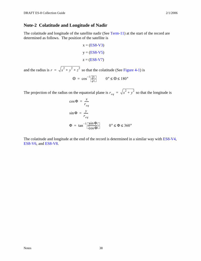
DRAFT ES-8 Collection Guide 2/1/2006
Notes 38
Note-2 Colatitude and Longitude of Nadir
The colatitude and longitude of the satellite nadir (See Term-11) at the start of the record are determined as follows. The position of the satellite is
x = (ES8-V3)
y = (ES8-V5)
z = (ES8-V7)
and the radius is so that the colatitude (See Figure 4-1) is
The projection of the radius on the equatorial plane is so that the longitude is
The colatitude and longitude at the end of the record is determined in a similar way with ES8-V4, ES8-V6, and ES8-V8.
r x2
y2
z2
+ +=
Θ cos 1– zr--
= 0° Θ≤ 180°≤
req x2
y2
+=
Φcos xreq-------=
Φsin yreq-------=
Φ tan 1– ΦsinΦcos
------------- = 0° Φ≤ 360°≤
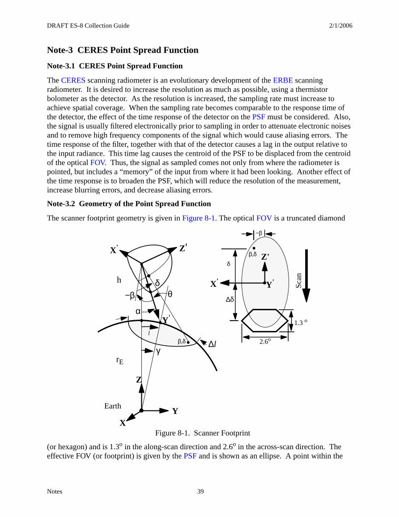
DRAFT ES-8 Collection Guide 2/1/2006
Notes 39
Note-3 CERES Point Spread Function
Note-3.1 CERES Point Spread Function
The CERES scanning radiometer is an evolutionary development of the ERBE scanning radiometer. It is desired to increase the resolution as much as possible, using a thermistor bolometer as the detector. As the resolution is increased, the sampling rate must increase to achieve spatial coverage. When the sampling rate becomes comparable to the response time of the detector, the effect of the time response of the detector on the PSF must be considered. Also, the signal is usually filtered electronically prior to sampling in order to attenuate electronic noises and to remove high frequency components of the signal which would cause aliasing errors. The time response of the filter, together with that of the detector causes a lag in the output relative to the input radiance. This time lag causes the centroid of the PSF to be displaced from the centroid of the optical FOV. Thus, the signal as sampled comes not only from where the radiometer is pointed, but includes a “memory” of the input from where it had been looking. Another effect of the time response is to broaden the PSF, which will reduce the resolution of the measurement, increase blurring errors, and decrease aliasing errors.
Note-3.2 Geometry of the Point Spread Function
The scanner footprint geometry is given in Figure 8-1. The optical FOV is a truncated diamond
(or hexagon) and is 1.3o in the along-scan direction and 2.6o in the across-scan direction. The effective FOV (or footprint) is given by the PSF and is shown as an ellipse. A point within the
X'
Y'
Z'
X' Y'
Z'
δ
α
−β θ
∆l
rE
h
1.3 o
2.6o
Figure 8-1. Scanner Footprint
γ
∆δ
β,δ
β,δ
δ
−β
l
Sca
n
XY
Z
Earth
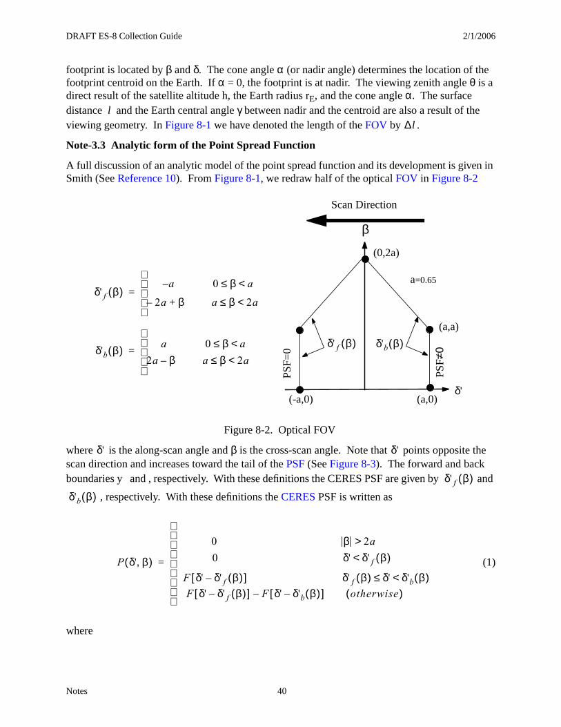
DRAFT ES-8 Collection Guide 2/1/2006
Notes 40
footprint is located by β and δ. The cone angle α (or nadir angle) determines the location of the footprint centroid on the Earth. If α = 0, the footprint is at nadir. The viewing zenith angle θ is a direct result of the satellite altitude h, the Earth radius rE, and the cone angle α. The surface distance l and the Earth central angle γ between nadir and the centroid are also a result of the viewing geometry. In Figure 8-1 we have denoted the length of the FOV by .
Note-3.3 Analytic form of the Point Spread Function
A full discussion of an analytic model of the point spread function and its development is given in Smith (See Reference 10). From Figure 8-1, we redraw half of the optical FOV in Figure 8-2
where is the along-scan angle and β is the cross-scan angle. Note that points opposite the scan direction and increases toward the tail of the PSF (See Figure 8-3). The forward and back boundaries y and , respectively. With these definitions the CERES PSF are given by and
, respectively. With these definitions the CERES PSF is written as
(1)
where
∆l
δ' f β( )
(a,0)(-a,0)
(a,a)
(0,2a)
β
δ'b β( )
Figure 8-2. Optical FOV
a=0.65
Scan Direction
PSF=
0
PSF≠
0
δ'
δ' f β( )a 0 β a<≤–
2a– β+ a β 2a<≤
=
δ'b β( ) a 0 β a<≤2a β– a β 2a<≤
=
δ' δ'
δ' f β( )
δ'b β( )
P δ' β,( )
0 β 2a>0 δ' δ' f β( )<
F δ' δ' f β( )–[ ] δ' f β( ) δ' δ'b β( )<≤F δ' δ' f β( )–[ ] F δ' δ'b β( )–[ ]– otherwise( )
=
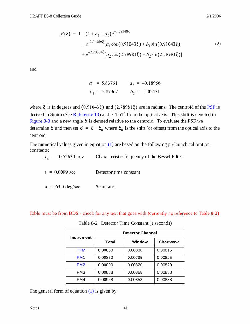
DRAFT ES-8 Collection Guide 2/1/2006
Notes 41
(2)
and
where is in degrees and and are in radians. The centroid of the PSF is
derived in Smith (See Reference 10) and is 1.51o from the optical axis. This shift is denoted in Figure 8-3 and a new angle is defined relative to the centroid. To evaluate the PSF we
determine and then set where is the shift (or offset) from the optical axis to the
centroid.
The numerical values given in equation (1) are based on the following prelaunch calibration constants:
Characteristic frequency of the Bessel Filter
Detector time constant
Scan rate
Table must be from BDS - check for any text that goes with (currently no reference to Table 8-2)
The general form of equation (1) is given by
Table 8-2. Detector Time Constant (τ seconds)
InstrumentDetector Channel
Total Window Shortwave
PFM 0.00860 0.00830 0.00815
FM1 0.00850 0.00795 0.00825
FM2 0.00800 0.00820 0.00820
FM3 0.00888 0.00868 0.00838
FM4 0.00928 0.00858 0.00888
F ξ( ) 1 1 a1 a2+ +( )e1.78348– ξ
–=
e3.04050ξ–
a1 0.91043ξ( )cos b1 0.91043ξ( )sin+[ ]+
e2.20860ξ–
a2 2.78981ξ( )cos b2 2.78981ξ( )sin+[ ]+
a1 5.83761= a2 0.18956–=
b1 2.87362= b2 1.02431=
ξ 0.91043ξ( ) 2.78981ξ( )
δδ δ' δ δ0+= δ0
f c 10.5263 hertz=
τ 0.0089 sec=
α 63.0 deg/sec=
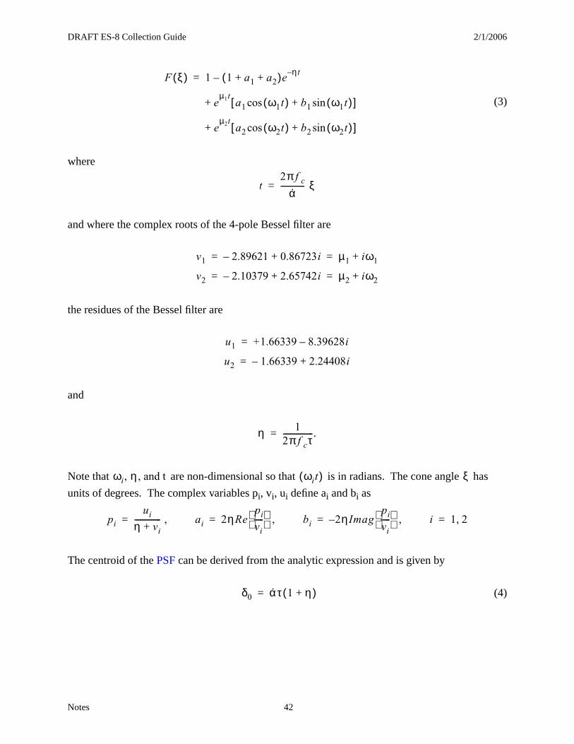
DRAFT ES-8 Collection Guide 2/1/2006
Notes 42
(3)
where
and where the complex roots of the 4-pole Bessel filter are
the residues of the Bessel filter are
and
.
Note that are non-dimensional so that is in radians. The cone angle has
units of degrees. The complex variables pi, vi, ui define ai and bi as
The centroid of the PSF can be derived from the analytic expression and is given by
(4)
F ξ( ) 1 1 a1 a2+ +( )eη– t
–=
eµ1t
a1 ω1t( )cos b1 ω1t( )sin+[ ]+
eµ2t
a2 ω2t( )cos b2 ω2t( )sin+[ ]+
t2π f c
α------------- ξ=
v1 2.89621– 0.86723i+ µ1 iω1+= =
v2 2.10379– 2.65742i+ µ2 iω2+= =
u1 +1.66339 8.39628i–=
u2 1.66339– 2.24408i+=
η 12π f cτ----------------=
ωi, η , and t ωit( ) ξ
pi
ui
η vi+-------------- ,= ai 2ηRe
pi
vi-----
,= bi 2– η Imagpi
vi-----
,= i 1 2,=
δ0 α τ 1 η+( )=
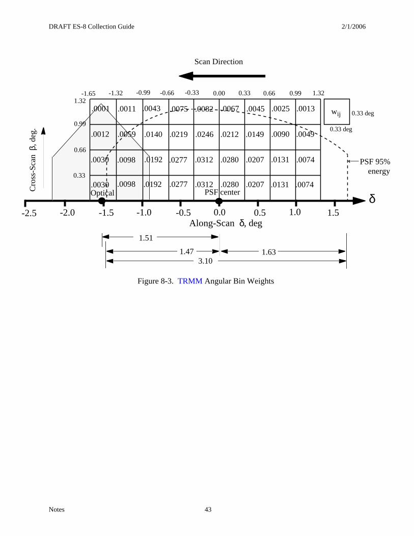
DRAFT ES-8 Collection Guide 2/1/2006
Notes 43
-1.65
.0280.0312Cro
ss-S
can
β, d
eg.
PSF center
-2.0 -1.0 1.00.0
Scan Direction
-0.5-1.5 0.5 1.5
3.101.631.47
Along-Scan δ, deg
wij
0.33 deg
0.33 deg
0.00 0.990.33 0.66 1.32-0.33-0.66-0.99-1.32
0.33
0.66
0.99
1.32
.0280
.0212
.0067
.0090
.0013.0025
.0149
.0045
.0131.0207
.0207
.0049
.0131 .0074
.0074
.0011
.0219
.0075
.0312
.0246
.0082.0043
.0192 .0277
.0277.0192.0098
.0098
.0059 .0140
Optical
PSF 95% energy
.0030
.0030
.0012
.0001
-2.5
1.51
δ
Figure 8-3. TRMM Angular Bin Weights
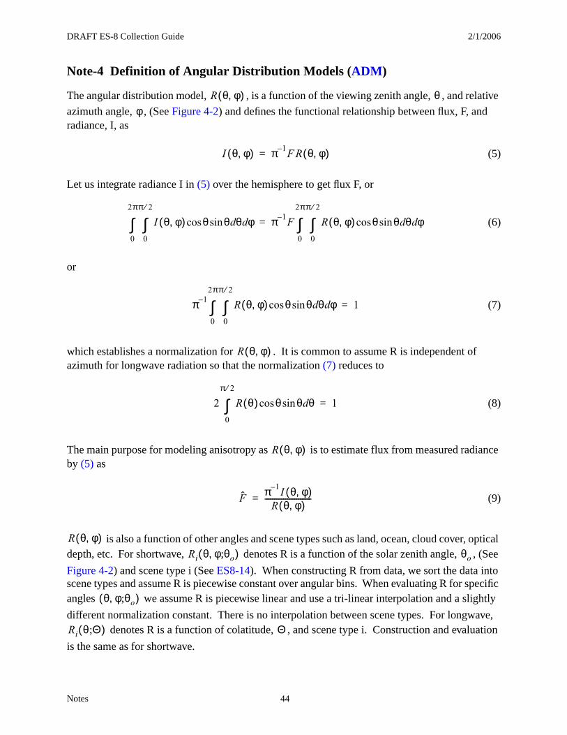
DRAFT ES-8 Collection Guide 2/1/2006
Notes 44
Note-4 Definition of Angular Distribution Models (ADM)
The angular distribution model, , is a function of the viewing zenith angle, , and relative
azimuth angle, , (See Figure 4-2) and defines the functional relationship between flux, F, and radiance, I, as
(5)
Let us integrate radiance I in (5) over the hemisphere to get flux F, or
(6)
or
(7)
which establishes a normalization for . It is common to assume R is independent of azimuth for longwave radiation so that the normalization (7) reduces to
(8)
The main purpose for modeling anisotropy as is to estimate flux from measured radiance by (5) as
(9)
is also a function of other angles and scene types such as land, ocean, cloud cover, optical depth, etc. For shortwave, denotes R is a function of the solar zenith angle, , (See
Figure 4-2) and scene type i (See ES8-14). When constructing R from data, we sort the data into scene types and assume R is piecewise constant over angular bins. When evaluating R for specific angles we assume R is piecewise linear and use a tri-linear interpolation and a slightly
different normalization constant. There is no interpolation between scene types. For longwave, denotes R is a function of colatitude, , and scene type i. Construction and evaluation
is the same as for shortwave.
R θ φ,( ) θφ
I θ φ,( ) π 1–F R θ φ,( )=
I θ φ,( ) θ θsincos θd φd
0
π 2⁄
∫0
2π
∫ π 1–F R θ φ,( ) θ θsincos θd φd
0
π 2⁄
∫0
2π
∫=
π 1–R θ φ,( ) θ θsincos θd φd
0
π 2⁄
∫0
2π
∫ 1=
R θ φ,( )
2 R θ( ) θ θsincos θd
0
π 2⁄
∫ 1=
R θ φ,( )
F π 1–I θ φ,( )
R θ φ,( )-------------------------=
R θ φ,( )Ri θ φ θo;,( ) θo
θ φ θo;,( )
Ri θ Θ;( ) Θ
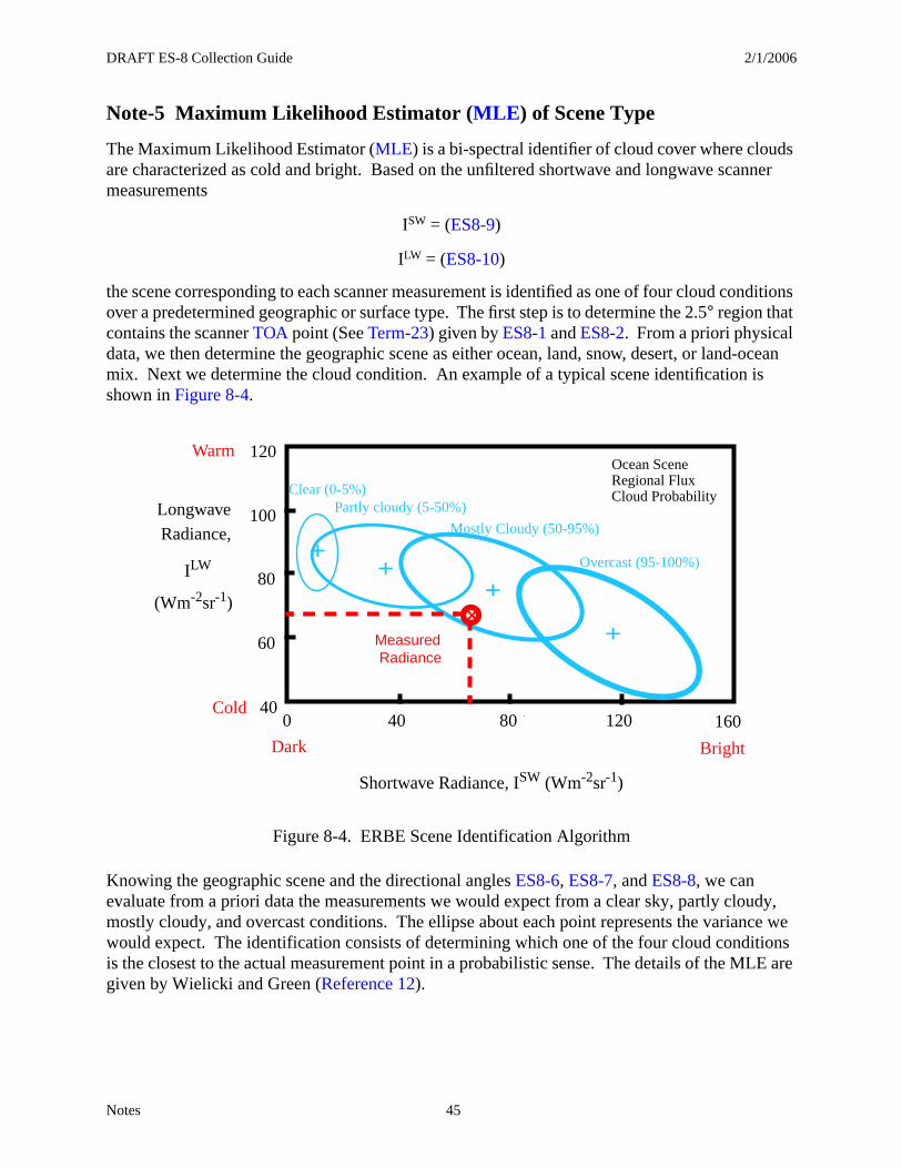
DRAFT ES-8 Collection Guide 2/1/2006
Notes 45
Note-5 Maximum Likelihood Estimator (MLE) of Scene Type
The Maximum Likelihood Estimator (MLE) is a bi-spectral identifier of cloud cover where clouds are characterized as cold and bright. Based on the unfiltered shortwave and longwave scanner measurements
ISW = (ES8-9)
ILW = (ES8-10)
the scene corresponding to each scanner measurement is identified as one of four cloud conditions over a predetermined geographic or surface type. The first step is to determine the 2.5° region that contains the scanner TOA point (See Term-23) given by ES8-1 and ES8-2. From a priori physical data, we then determine the geographic scene as either ocean, land, snow, desert, or land-ocean mix. Next we determine the cloud condition. An example of a typical scene identification is shown in Figure 8-4.
Knowing the geographic scene and the directional angles ES8-6, ES8-7, and ES8-8, we can evaluate from a priori data the measurements we would expect from a clear sky, partly cloudy, mostly cloudy, and overcast conditions. The ellipse about each point represents the variance we would expect. The identification consists of determining which one of the four cloud conditions is the closest to the actual measurement point in a probabilistic sense. The details of the MLE are given by Wielicki and Green (Reference 12).
Figure 8-4. ERBE Scene Identification Algorithm
Shortwave Radiance, ISW (Wm-2sr-1)
LongwaveRadiance,
ILW
Dark Bright
Cold
Warm
Clear (0-5%)Partly cloudy (5-50%)
Mostly Cloudy (50-95%)
Overcast (95-100%)
Ocean SceneRegional FluxCloud Probability
+
++
+
xMeasuredRadiance
(Wm-2sr-1)
40 80 1600 120
100
80
60
40
120
DRAFT ES-8 Collection Guide 2/1/2006
Notes 46
Note-6 Spectral Correction Algorithm
The radiances as measured by the CERES instruments are filtered radiances and the spectral cor-rection algorithm unfilters these radiances. The desired unfiltered radiances are defined by
where λ (µm) is the wavelength, λ1 = 8.1 and λ2 = 11.8, and and are the reflected and emit-
ted components of the total observed radiance or . The filtered measurements are
modeled as
where is the normalized spectral response function . The spectral response func-
tion for CERES_ TRMM is shown in the Figure 8-5 and represents the spectral throughput of the individual detector’s optical elements determined from laboratory measurements. An estimate of the unfiltered SW and WN radiances are determined from the filtered radiance measurements as follows:
where a0, a1, a2, b0, b1, and b2 are theoretically derived regression coefficients that depend on
scene type and viewing geometry. represents the reflected portion of the filtered SW radi-
ance measurement and is given by where is the emitted thermal por-
tion of and is estimated from using a pre-determined empirical 2nd order polynomial
expression relating nighttime and measurements. For CERES_ TRMM the least-
square fit is given by:
ISW
I λr λd
0
∞∫=
ILW
I λe λd
0
∞∫=
IWN 1
λ2 λ1–----------------- I λ
e λdλ1
λ2
∫=
I λr
I λe
I λ I λr
I λe
+=
m fi
SλiI λ λd
0
∞∫= i SW, TOT=
m fi 1
λ2 λ1–----------------- Sλ
iI λ λd
0
∞∫= i WN=
Sλi 0 Sλ
i 1≤ ≤( )
ISW
a0 a1 m fSW r( ) a2 m f
SW r( )2
+ +=
IWN
b0 b1 m fWN( ) b2 m f
WN( )2
+ +=
m fSW r
m fSW r m f
SWm f
SW e–= m fSW e
m fSW
m fWN
m fSW
m fWN
m fSW e k0 k1 m f
WN( ) k2 m fWN( )
2+ +=
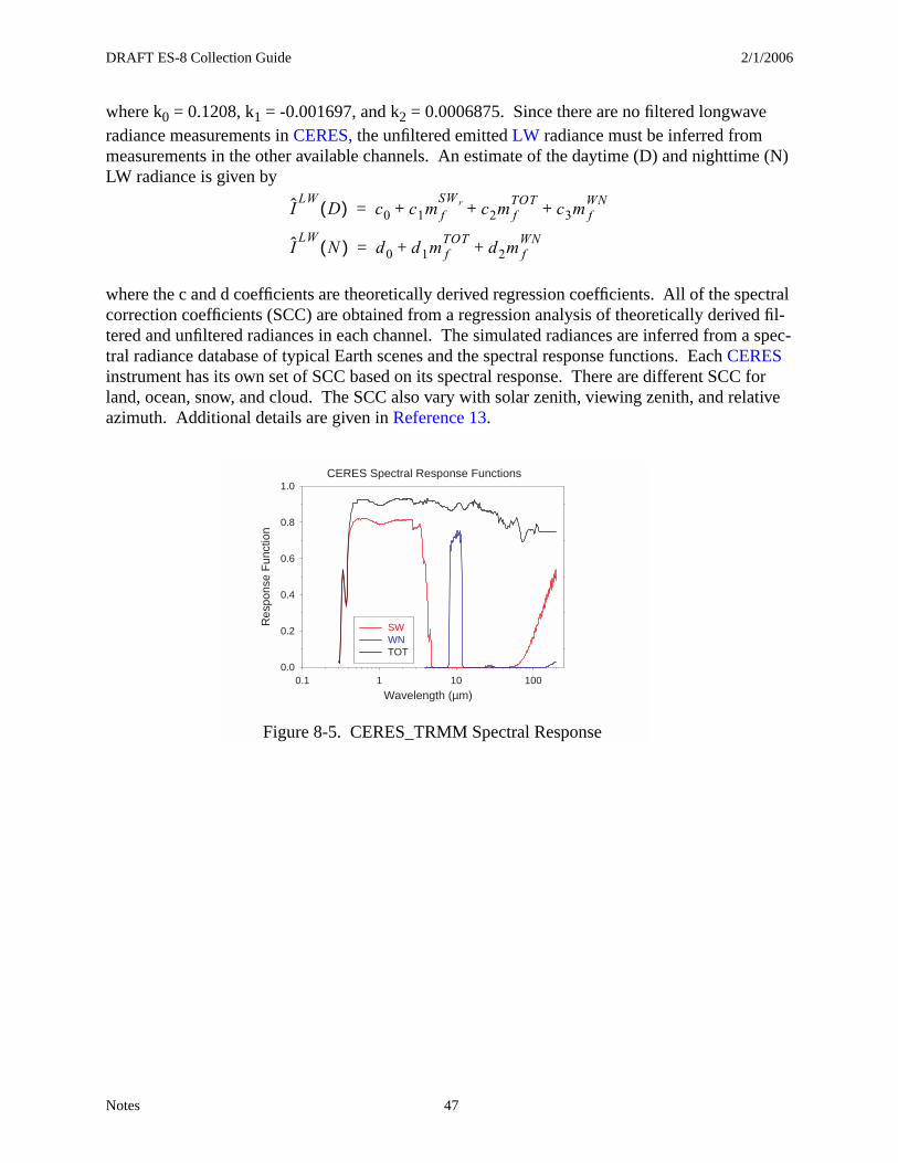
DRAFT ES-8 Collection Guide 2/1/2006
Notes 47
where k0 = 0.1208, k1 = -0.001697, and k2 = 0.0006875. Since there are no filtered longwave radiance measurements in CERES, the unfiltered emitted LW radiance must be inferred from measurements in the other available channels. An estimate of the daytime (D) and nighttime (N) LW radiance is given by
where the c and d coefficients are theoretically derived regression coefficients. All of the spectral correction coefficients (SCC) are obtained from a regression analysis of theoretically derived fil-tered and unfiltered radiances in each channel. The simulated radiances are inferred from a spec-tral radiance database of typical Earth scenes and the spectral response functions. Each CERES instrument has its own set of SCC based on its spectral response. There are different SCC for land, ocean, snow, and cloud. The SCC also vary with solar zenith, viewing zenith, and relative azimuth. Additional details are given in Reference 13.
ILW
D( ) c0 c1m fSW r c2m f
TOTc3m f
WN+ + +=
ILW
N( ) d0 d1m fTOT
d2m fWN
+ +=
CERES Spectral Response Functions
Wavelength (µm)0.1 1 10 100
Res
pons
e F
unct
ion
0.0
0.2
0.4
0.6
0.8
1.0
SWWNTOT
Figure 8-5. CERES_TRMM Spectral Response
DRAFT ES-8 Collection Guide 2/1/2006
Application of the Data Set 48
9.0 Application of the Data Set
The ES-8 data product provides time and position data on a record-level basis and measurement-level data including filtered, unfiltered, TOA, and scene identification data (See Section 1.4).
10.0 Future Modifications and Plans
Modifications to the ES-8 product are driven by validation results and any Terra related parameters. The Langley ASDC provides users notification of changes.
11.0 Software Description
There are Fortran90 and C read programs available at the Langley ASDC. The programs were designed to run on a Unix workstation and can be compiled with a Fortran90 or C compiler, respectively.{Pointer to ASDC read program}
12.0 Contact Data Center/Obtain Data
NASA Langley Atmospheric Sciences Data Center Telephone: (757) 864-8656Science, User and Data Service Office FAX: (757) 864-8807NASA Langley Research Center E-mail: [email protected] Stop 157D URL: http://eosweb.larc.nasa.gov/2 South Wright StreetHampton, VA 23681-2199USA
13.0 Output Products and Availability
Several media types are supported by the Langley Web Order Tool. Data can be downloaded from the Web or via FTP. Alternatively, data can be ordered on media tapes. The media tapes supported are 4mm 2Gb (90m), 8mm 2Gb (8200), 8mm 5Gb (8500), and 8mm 7Gb (8500c).
Data ordered via the Web or via FTP can be downloaded in either Uncompressed mode or in UNIX Compressed mode. Data written to media tape (in either Uncompressed mode or in UNIX Compressed mode) is in UNIX TAR format.
DRAFT ES-8 Collection Guide 2/1/2006
References 49
14.0 References
1. NASA Langley Atmospheric Science Data Hierarchical Data Format Web site {URL = http://eosweb/HBDOCS/hdf.html}.
2. Clouds and the Earth’s Radiant Energy System (CERES) Data Management System Data Products Catalog Release 3, Version 1, July 1998 {URL = http://asd-www.larc.nasa.gov/DPC/DPC.html}.
3. TRW DRL 64, 55067.300.008E; In-flight Measurement Analysis (Rev. E), March 1997.
4. Clouds and the Earth’s Radiant Energy System (CERES) Algorithm Theoretical Basis Document, Instrument Geolocate and Calibrate Earth Radiances (Subsystem 1.0), Release 2.2, June 1997 {URL = http://asd-www.larc.nasa.gov/ATBD/ATBD.html}.
5. Clouds and the Earth’s Radiant Energy System (CERES) Algorithm Theoretical Basis Document, ERBE-like to Instantaneous Fluxes (Subsystem 2.0), Rel. 2.2, June 2, 1997 {URL = http://asd-www.larc.nasa.gov/ATBD/ATBD.html}.
6. Clouds and the Earth’s Radiant Energy System (CERES) Data Management System Software Requirements Document, ERBE-like Inversion to Instantaneous TOA and Surface Fluxes (Subsystem 2.0), Release 1 Version 1, November 1994 {URL = http://asd-www.larc.nasa.gov/SRD/SRD.html}.
7. Clouds and the Earth’s Radiant Energy System (CERES) Validation Plan, ERBE-like Inversion to Instantaneous TOA Flux (Subsystem 2.0), Release 2.2, July 1997 {URL = http://asd-www.larc.nasa.gov/validation/valid_doc.html}
8. Blackadar, Alfred: A Computer Almanac, Weatherwise, Vol 37, No 5, October 1984, p. 257-260.
9. Jefferys, William H.: Julian Day Numbers {URL = http://quasar.as.utexas.edu/BillInfo/JulianDatesG.html}.
10. Smith, G. L., 1994: Effects of time response on the point spread function of a scanning radiometer, Appl. Opt., Vol. 33, No. 30, 7031-7037.
11. Software Bulletin “CERES Metadata Requirements for LaTIS,” Revision 1, January 7, 1998 {URL = http://asd-www.larc.nasa.gov/ceres/bulletins.html}.
12. Wielicki, B. A., and R. N. Green, 1989: Cloud identification for ERBE radiation flux retrieval, J. Appl. Meteor., 28, 1133-1146.
13. Loeb, N. G., Priestley, K. J., Kratz, D. P., Geier, E. B., Green, R. N., Wielicki, B. A., Hinton, P. O’R., and Nolan, S. K.: Determination of Unfiltered Radiances from CERES. Submitted to Journal of Applied Meteorology, 2000.
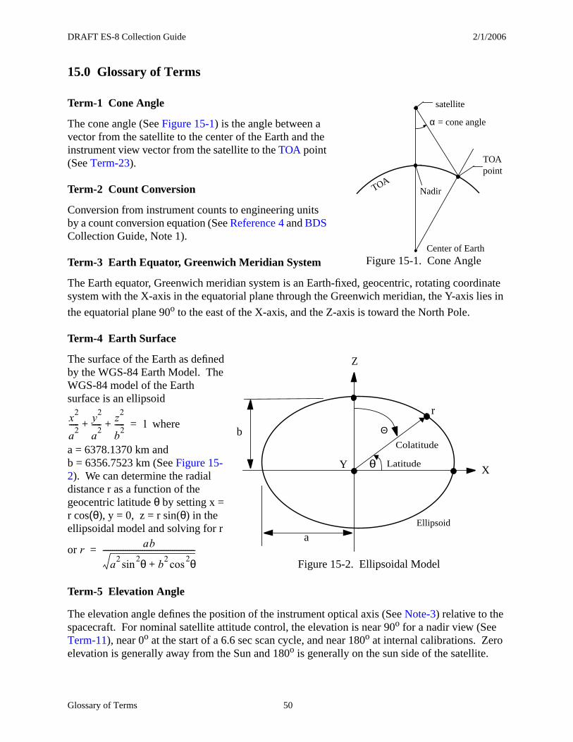
DRAFT ES-8 Collection Guide 2/1/2006
Glossary of Terms 50
15.0 Glossary of Terms
Term-1 Cone Angle
The cone angle (See Figure 15-1) is the angle between a vector from the satellite to the center of the Earth and the instrument view vector from the satellite to the TOA point (See Term-23).
Term-2 Count Conversion
Conversion from instrument counts to engineering units by a count conversion equation (See Reference 4 and BDS Collection Guide, Note 1).
Term-3 Earth Equator, Greenwich Meridian System
The Earth equator, Greenwich meridian system is an Earth-fixed, geocentric, rotating coordinate system with the X-axis in the equatorial plane through the Greenwich meridian, the Y-axis lies in
the equatorial plane 90o to the east of the X-axis, and the Z-axis is toward the North Pole.
Term-4 Earth Surface
The surface of the Earth as defined by the WGS-84 Earth Model. The WGS-84 model of the Earth surface is an ellipsoid
where
a = 6378.1370 km and b = 6356.7523 km (See Figure 15-2). We can determine the radial distance r as a function of the geocentric latitude θ by setting x = r cos(θ), y = 0, z = r sin(θ) in the ellipsoidal model and solving for r
or
Term-5 Elevation Angle
The elevation angle defines the position of the instrument optical axis (See Note-3) relative to the spacecraft. For nominal satellite attitude control, the elevation is near 90o for a nadir view (See Term-11), near 0o at the start of a 6.6 sec scan cycle, and near 180o at internal calibrations. Zero elevation is generally away from the Sun and 180o is generally on the sun side of the satellite.
Figure 15-1. Cone Angle
TOA
satellite
TOApoint
α = cone angle
Nadir
Center of Earth
XY
Z
a
b
θ
Ellipsoid
Figure 15-2. Ellipsoidal Model
r
Θ
Latitude
Colatitude
x2
a2
----- y2
a2
----- z2
b2
-----+ + 1=
r ab
a2 θ2sin b
2 θ2cos+
-------------------------------------------------=
DRAFT ES-8 Collection Guide 2/1/2006
Glossary of Terms 51
Term-6 Field-of-View
The instrument field-of-view (FOV) is determined by the instrument point spread function (See Term-12) and is defined as the minimum area over the radiation field from which 95% of the mea-sured radiance is obtained. For the purpose of determining full FOV coverage of the Earth surface (See ES8-18), the forward edge of the FOV is offset 1.7 deg at the satellite in front of the PSF cen-troid while the trailing edge is offset 1.7 deg behind the centroid. (See Note-3).
Term-7 Fixed azimuth plane scan (FAPS)
Term-8 Geocentric Colatitude
Term-9 Granule
The ES-8 product is one day or 24 hours of data and is called a granule. Or, a granule is all records (See Term-14) for a day.
Term-10 Julian Date
Julian Date is a continuous count of time in whole and fractional days elapsed at the Greenwich meridian since noon on January 1, 4714 BCE. (See Note-1)
Term-11 Nadir
The point on the Earth surface below the satellite or the intersection point of a line from the center of the Earth to the satellite and the Earth surface (See Figure 15-1).
Term-12 Point Spread Function
A Point Spread Function (PSF) is a two-dimensional bell-shaped function that defines the CERES instrument response to the viewed radiation field. Due to the response time, the radiometer responds to a larger FOV than the optical FOV and the resulting PSF centroid lags the optical FOV centroid by more than a degree of cone angle (See Term-1) for normal scan rates (See Note-3).
Term-13 Rapid Retrace (or Fast Return)
Rapid retrace is defined as a much faster than nominal elevation, or cone angle, scan rate. The
rapid retrace rate is currently defined as 249.69 10 deg sec -1. During the Short Elevation Scan cycle, there are two portions of the scan cycle where the CERES instrument sweeps across the
Earth at a rate of approximately 249 deg sec -1. These are examples of rapid retrace (See Figure 15-3).
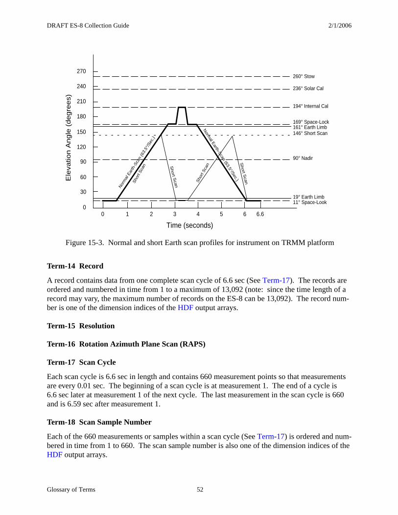
DRAFT ES-8 Collection Guide 2/1/2006
Glossary of Terms 52
Term-14 Record
A record contains data from one complete scan cycle of 6.6 sec (See Term-17). The records are ordered and numbered in time from 1 to a maximum of 13,092 (note: since the time length of a record may vary, the maximum number of records on the ES-8 can be 13,092). The record num-ber is one of the dimension indices of the HDF output arrays.
Term-15 Resolution
Term-16 Rotation Azimuth Plane Scan (RAPS)
Term-17 Scan Cycle
Each scan cycle is 6.6 sec in length and contains 660 measurement points so that measurements are every 0.01 sec. The beginning of a scan cycle is at measurement 1. The end of a cycle is 6.6 sec later at measurement 1 of the next cycle. The last measurement in the scan cycle is 660 and is 6.59 sec after measurement 1.
Term-18 Scan Sample Number
Each of the 660 measurements or samples within a scan cycle (See Term-17) is ordered and num-bered in time from 1 to 660. The scan sample number is also one of the dimension indices of the HDF output arrays.
Time (seconds)
Ele
vatio
n A
ngle
(degre
es)
Short S
can
260° Stow
236° Solar Cal
194° Internal Cal
169° Space-Lock161° Earth Limb146° Short Scan
90° Nadir
19° Earth Limb11° Space-Look
0 1 2 3 4 5 6 6.6
Norm
al Earth-S
can (63.5°/Sec.)
Sho
rt S
can
Sho
rt S
can S
hort S
can
Nor
mal
Ear
th-S
can
(63.
5°/S
ec.)
0
30
60
90
120
150
180
210
240
270
Figure 15-3. Normal and short Earth scan profiles for instrument on TRMM platform
DRAFT ES-8 Collection Guide 2/1/2006
Glossary of Terms 53
Term-19 Scientific Data Set
A Scientific Data Set (SDS) is an HDF structure. It is a collection (or grouping) of parameters that have the same data type such as 8, 16, or 32-bit integers or 32, or 64-bit floating point numbers. The ES-8 SDS’s each contain only one parameter. The SDS is an array of values and for ES-8 this corresponds to a two dimensional array of all values of a certain parameter for a day. The dimensions of the array correspond to the number of footprints (660) within a record (scan cycle) and the number of records within the granule. In general, an SDS is a multi-dimensional array. It has dimension records and data type which describe it. The dimensions specify the shape and size of the SDS array. Each dimension has its own attributes.
Term-20 Spectral Correction
The Spectral Correction Coefficients (SCC) represent a regression between theoretical filtered radiances and theoretical unfiltered radiances and are used to unfilter the CERES radiances. Each CERES instrument has its own set of SCC based on its spectral response. There are different SCC for land, ocean, snow, and cloud. The SCC also vary with solar zenith, viewing zenith, and rela-tive azimuth. (See Note-6)
Term-21 Subsolar Point
The point at which a vector from the center of the Earth to the Sun intersects the TOA (See Term-22).
Term-22 Top-of-the-Atmosphere
The Top-of-the-Atmosphere (TOA) is a surface approximately 30 km above the Earth surface
(See Term-4). Specifically, the TOA is an ellipsoid where a = 6408.1370 km
and b = 6386.6517 km (See Figure 15-2). We can determine the radial distance r as a function of the geocentric latitude θc by setting x = r cos(θ), y = 0, z = r sin(θ) in the ellipsoidal model and solving for r or
Term-23 TOA Point
The viewed point at the TOA, or the point at which the PSF (See Term-12) centroid intersects the TOA (See Term-22).
Term-24 Vertex Data
A Vertex data (Vdata) set is an HDF structure. It is a collection (or grouping) of parameters that have different data types such as 8, 16, or 32-bit integers, floating point numbers, text, etc. In general, Vdata is a table of parameters of varying data type. Specifically stated, a Vdata is a customized table, comprised of a collection of similar records (rows) whose values are stored in
x2
a2
----- y2
a2
----- z2
b2
-----+ + 1=
r ab
a2 θ2sin b
2 θ2cos+
-------------------------------------------------=

DRAFT ES-8 Collection Guide 2/1/2006
Acronyms and Units 54
one or more fixed length fields (columns) where individual fields can have their own data type. The ES-8 contains 20 record-level parameters, each of which is written into a separate Vdata. Therefore, an ES-8 record-level Vdata contains a single field (column) which has multiple values (rows) such that one value exists for each record (scan cycle) within the granule. The ES-8 also contains a CERES_metadata Vdata which contains numerous parameters (columns) and each parameter has only one value per granule. A Vdata is uniquely identified by a name, a class, and individual field names. The Vdata class identifies the purpose or use of its data.
16.0 Acronyms and Units
16.1 CERES Acronyms
ADM Angular Distribution ModelAPID Application IdentifierAPD Aerosol Profile DataATBD Algorithm Theoretical Basis DocumentAVG Monthly Regional Radiative Fluxes and CloudsAVHRR Advanced Very High Resolution RadiometerBCE Before Current EraBDS BiDirectional Scan (data product)CADM CERES Angular Distribution ModelCER CERESCERES Clouds and the Earth’s Radiant Energy SystemCID Cloud Imager Data (data product)CRH Clear Reflectance History (data product)CRS Clouds and Radiative Swath (data product)CW Cable WrapDAAC Distributed Active Archive CenterDAC Digital to Analog ConverterDAO Data Assimilation OfficeDAP Data Acquisition microProcessorDMA Direct Memory AccessDMS Data Management SystemDPC Data Products CatalogECR Earth-Centered RotatingEDDB ERBE-Like Daily Database ProductEDOS EOS Data Operations SystemEOS Earth Observing SystemEOS AM EOS Morning Crossing Mission (Renamed Terra)EOS PM EOS Afternoon Crossing Mission (Renamed Aqua)EOSDIS Earth Observing System Data and Information SystemERBE Earth Radiation Budget ExperimentERBS Earth Radiation Budget SatelliteFAPS Fixed Azimuth Plane Scan

DRAFT ES-8 Collection Guide 2/1/2006
Acronyms and Units 55
FM Flight ModelFOV Field-of-View (See Term-6)FSW Monthly Single Satellite Fluxes and CloudsFTP File Transfer ProtocolGAP Gridded Analysis ProductGB GigabyteGEO Geostationary Narrowband RadiancesGMS Geostationary Meteorological SatelliteGGEO Gridded Geostationary Narrowband RadiancesGMT Greenwich Mean TimeGOES Geostationary Operational Environmental SatelliteH HighHDF Hierarchical Data FormatIES Instrument Earth Scans (data product)IGBP International Geosphere Biosphere ProgrammeINSTR InstrumentISCCP International Satellite Cloud Climatology ProjectIWC Ice Water ContentLaRC Langley Research CenterLaTIS Langley TRMM Information SystemL LowLM Lower MiddleLW LongwaveLWC Liquid Water ContentMAM Mirror Attenuator MosaicMB MegabyteMETEOSAT Meteorological SatelliteMISR Multi-angle Imaging SpectroRadiometerMLE Maximum Likelihood EstimatorMOA Meteorological, Ozone, and Aerosols (data product)MODIS Moderate Resolution Imaging SpectrometerMWH Microwave Humidity (data product)NASA National Aeronautics and Space AdministrationNOAA National Oceanic and Atmospheric AdministrationOPD Ozone Profile Data (data product)PFM Prototype Flight Model (on TRMM)PSA Product Specific AttributePSF Point Spread Function (See Term-12)QA Quality AssessmentRAPS Rotating Azimuth Plane ScanSARB Surface and Atmospheric Radiation BudgetSBUV-2 Solar Backscatter Ultraviolet/Version 2SDS Scientific Data Set (See Term-19)SFC Hourly Gridded Single Satellite TOA/Surface Fluxes and Clouds (data product)SPS Solar Presence SensorSRB Surface Radiation Budget
DRAFT ES-8 Collection Guide 2/1/2006
Acronyms and Units 56
SRBAVG Surface Radiation Budget Average (data product)SS SubsystemSSF Single Satellite CERES Footprint TOA and Surface Fluxes, Clouds (data product)SSM/I Special Sensor Microwave/ImagerSURFMAP Surface MapSW ShortwaveSWICS Shortwave Internal Calibration SourceSYN Synoptic Radiative Fluxes and CloudsTBD To Be DeterminedTISA Time Interpolation and Spatial AveragingTMI TRMM Microwave ImagerTOA Top-of-the-Atmosphere (See Term-22)TOT TotalTRMM Tropical Rainfall Measuring MissionUM Upper MiddleURL Uniform Resource LocatorUT Universal TimeUTC Universal Time CodeVIRS Visible Infrared ScannerWN WindowWWW World Wide WebZAVG Monthly Zonal and Global Average Radiative Fluxes and Clouds (data product)
16.2 CERES Units
Unit Definitions
Units Definition
AU Astronomical Unit
cm centimeter
count count, counts
day day, Julian date
deg degree
deg sec-1 degrees per second
du Dobson units
fraction fraction 0..1
g kg-1 gram per kilogram
g m-2 gram per square meter
hhmmss hour, minute, second
hour hour
hPa hectoPascals
DRAFT ES-8 Collection Guide 2/1/2006
Acronyms and Units 57
in-oz inch-ounce
K Kelvin
km kilometer, kilometers
km sec-1 kilometers per second
m meter
mA milliamp, milliamps
micron micrometer, micron
msec millisecond
mW cm-2sr-1µm-1 milliWatts per square centimeter per steradian per micron
m sec-1 meter per second
N/A not applicable, none, unitless, dimensionless
percent percent, percentage 0..100
rad radian
sec second
volt volt, volts
W h m-2 Watt hour per square meter
W2 m-4 square Watt per meter to the 4th
W m-2 Watt per square meter
W m-2sr-1 Watt per square meter per steradian
W m-2sr-1µm-1 Watt per square meter per steradian per micron
°C degrees centigrade
µm micrometer, micron
Units Definition
DRAFT ES-8 Collection Guide 2/1/2006
Document Information 58
17.0 Document Information
17.1 Document Creation Date - May 15, 1998
17.2 Document Review Date -
17.3 Document Revision Date
Month 1999 Comment
17.4 Document ID
LD_007_010_001_00_00_0_yyyymmdd (Release Date) [get this from ASDC User Services]
17.5 Citation
Please provide a reference to the following paper when scientific results are published using the CERES XYZ TRMM data:
“Wielicki, B. A.; Barkstrom, B.R.; Harrison, E. F.; Lee III,R.B.; Smith, G.L.; and Cooper, J.E., 1996: Clouds and the Earth’s Radiant Energy System (CERES): An Earth Observing System Experiment, Bull. Amer. Meteor. Soc., 77, 853-868.”
When Langley Atmospheric Sciences Data Center (ASDC) data are used in a publication, the following acknowledgment is requested to be included:
“These data were obtained from the NASA Langley Research Center EOSDIS Distributed Active Archive Center.”
The Data Center at Langley requests two reprints of any published papers or reports which cite the use of data the Langley ASDC have distributed. This will help the ASDC to determine the use of data distributed, which is helpful in optimizing product development. It also helps the ASDC to keep product related references current.
17.6 Redistribution of Data
To assist the Langley ASDC in providing the best service to the scientific community, a notification is requested if these data are transmitted to other researchers.
17.7 Document Curator
The Langley ASDC Science, User & Data Services Office.
DRAFT ES-8 Collection Guide 2/1/2006
59
18.0 Index
[A], [B], [C], [D], [E], [F], [G], [H], [I], [J], [K], [L], [M], [N], [O], [P], [Q], [R], [S], [T], [U], [V], [W], [X], [Y], [Z]
A
Acronyms, list, 16.1 . . . . . . . . . . . . . . . . . . . . . . . . . . . . . . . . . . . . . . . . . . . . . . . . . . . . . . . . . . . . 54
ADMdefinition, Note-4 . . . . . . . . . . . . . . . . . . . . . . . . . . . . . . . . . . . . . . . . . . . . . . . . . . . . . . . . . . 44
Along-track scan (See azimuth scan plane, ES8-20, word 3) . . . . . . . . . . . . . . . . . . . . . . . . . . . . 22
Angleazimuth, ES8-8 . . . . . . . . . . . . . . . . . . . . . . . . . . . . . . . . . . . . . . . . . . . . . . . . . . . . . . . . . . . . 16colatitude (See Colatitude)cone, Term-1 . . . . . . . . . . . . . . . . . . . . . . . . . . . . . . . . . . . . . . . . . . . . . . . . . . . . . . . . . . . . . . 50elevation, Term-5 . . . . . . . . . . . . . . . . . . . . . . . . . . . . . . . . . . . . . . . . . . . . . . . . . . . . . . . . . . 50longitude (See Longitude)relative azimuth angle, ES8-8 . . . . . . . . . . . . . . . . . . . . . . . . . . . . . . . . . . . . . . . . . . . . . . . . . 16solar zenith, ES8-7 . . . . . . . . . . . . . . . . . . . . . . . . . . . . . . . . . . . . . . . . . . . . . . . . . . . . . . . . . 16viewing zenith, ES8-6 . . . . . . . . . . . . . . . . . . . . . . . . . . . . . . . . . . . . . . . . . . . . . . . . . . . . . . . 16
B
BDRF (See ADM)
Bidirectional function (See ADM)
C
CERESinstrument character name, Table A-1. . . . . . . . . . . . . . . . . . . . . . . . . . . . . . . . . . . . . . . . . . A-1point spread function, Note-3 . . . . . . . . . . . . . . . . . . . . . . . . . . . . . . . . . . . . . . . . . . . . . . . . . 39satellite character name, Table A-1. . . . . . . . . . . . . . . . . . . . . . . . . . . . . . . . . . . . . . . . . . . . A-1
ChannelSW, ES8-4 . . . . . . . . . . . . . . . . . . . . . . . . . . . . . . . . . . . . . . . . . . . . . . . . . . . . . . . . . . . . . . . . 15TOT, ES8-3 . . . . . . . . . . . . . . . . . . . . . . . . . . . . . . . . . . . . . . . . . . . . . . . . . . . . . . . . . . . . . . . 14WN, ES8-5 . . . . . . . . . . . . . . . . . . . . . . . . . . . . . . . . . . . . . . . . . . . . . . . . . . . . . . . . . . . . . . . 15
Citation for data use, 17.5 . . . . . . . . . . . . . . . . . . . . . . . . . . . . . . . . . . . . . . . . . . . . . . . . . . . . . . . 58
Clear area (See Scene type at observation)
Cloud fraction (See Scene type at observation)
Colatitudedefinition
Figure 4-1. . . . . . . . . . . . . . . . . . . . . . . . . . . . . . . . . . . . . . . . . . . . . . . . . . . . . . . . . . . . . 12Note-2 . . . . . . . . . . . . . . . . . . . . . . . . . . . . . . . . . . . . . . . . . . . . . . . . . . . . . . . . . . . . . . . 38
DRAFT ES-8 Collection Guide 2/1/2006
60
of observation at TOA, ES8-1 . . . . . . . . . . . . . . . . . . . . . . . . . . . . . . . . . . . . . . . . . . . . . . . . . 13of satellite, ES8-V15 . . . . . . . . . . . . . . . . . . . . . . . . . . . . . . . . . . . . . . . . . . . . . . . . . . . . . . . . 12of Sun, ES8-V19 . . . . . . . . . . . . . . . . . . . . . . . . . . . . . . . . . . . . . . . . . . . . . . . . . . . . . . . . . . . 13
Cone angle, Term-1 . . . . . . . . . . . . . . . . . . . . . . . . . . . . . . . . . . . . . . . . . . . . . . . . . . . . . . . . . . . . 50
Count conversion, Term-2 . . . . . . . . . . . . . . . . . . . . . . . . . . . . . . . . . . . . . . . . . . . . . . . . . . . . . . . 50
Cross-track scan (See azimuth scan plane, ES8-20, word 3) . . . . . . . . . . . . . . . . . . . . . . . . . . . . . 22
D
Datagranularity, 5.1 . . . . . . . . . . . . . . . . . . . . . . . . . . . . . . . . . . . . . . . . . . . . . . . . . . . . . . . . . . . . 30metadata, APPENDIX A . . . . . . . . . . . . . . . . . . . . . . . . . . . . . . . . . . . . . . . . . . . . . . . . . . . . A-1organization, 5.0 . . . . . . . . . . . . . . . . . . . . . . . . . . . . . . . . . . . . . . . . . . . . . . . . . . . . . . . . . . . 29use
citation, 17.5 . . . . . . . . . . . . . . . . . . . . . . . . . . . . . . . . . . . . . . . . . . . . . . . . . . . . . . . . . . . 58redistribution of data, 17.6 . . . . . . . . . . . . . . . . . . . . . . . . . . . . . . . . . . . . . . . . . . . . . . . . 58
Default fill values, 4.4 . . . . . . . . . . . . . . . . . . . . . . . . . . . . . . . . . . . . . . . . . . . . . . . . . . . . . . . . . . 28
E
EarthSun distance, ES8-V2 . . . . . . . . . . . . . . . . . . . . . . . . . . . . . . . . . . . . . . . . . . . . . . . . . . . . . . . 10surface model, Term-4 . . . . . . . . . . . . . . . . . . . . . . . . . . . . . . . . . . . . . . . . . . . . . . . . . . . . . . 50
Elevation angle, Term-5 . . . . . . . . . . . . . . . . . . . . . . . . . . . . . . . . . . . . . . . . . . . . . . . . . . . . . . . . . 50
ERBE 12 scene types, ES8-14 . . . . . . . . . . . . . . . . . . . . . . . . . . . . . . . . . . . . . . . . . . . . . . . . . . . . 19
ES8 headerES8-V1 Time at observation . . . . . . . . . . . . . . . . . . . . . . . . . . . . . . . . . . . . . . . . . . . . . . . . . . . 9ES8-V2 Earth-Sun distance at record start . . . . . . . . . . . . . . . . . . . . . . . . . . . . . . . . . . . . . . . 10ES8-V3 X component of satellite position at record start . . . . . . . . . . . . . . . . . . . . . . . . . . . 10ES8-V4 X component of satellite position at record end . . . . . . . . . . . . . . . . . . . . . . . . . . . . 10ES8-V5 Y component of satellite position at record start . . . . . . . . . . . . . . . . . . . . . . . . . . . 10ES8-V6 Y component of satellite position at record end . . . . . . . . . . . . . . . . . . . . . . . . . . . . 10ES8-V7 Z component of satellite position at record start . . . . . . . . . . . . . . . . . . . . . . . . . . . . 11ES8-V8 Z component of satellite position at record end . . . . . . . . . . . . . . . . . . . . . . . . . . . . 11ES8-V9 X component of satellite velocity at record start . . . . . . . . . . . . . . . . . . . . . . . . . . . 11ES8-V10 X component of satellite velocity at record end . . . . . . . . . . . . . . . . . . . . . . . . . . . 11ES8-V11 Y component of satellite velocity at record start . . . . . . . . . . . . . . . . . . . . . . . . . . 11ES8-V12 Y component of satellite velocity at record end . . . . . . . . . . . . . . . . . . . . . . . . . . . 11ES8-V13 Z component of satellite velocity at record start . . . . . . . . . . . . . . . . . . . . . . . . . . . 11ES8-V14 Z component of satellite velocity at record end . . . . . . . . . . . . . . . . . . . . . . . . . . . 12ES8-V15 Colatitude of satellite nadir at record start . . . . . . . . . . . . . . . . . . . . . . . . . . . . . . . 12ES8-V16 Colatitude of satellite nadir at record end . . . . . . . . . . . . . . . . . . . . . . . . . . . . . . . . 12ES8-V17 Longitude of satellite nadir at record start . . . . . . . . . . . . . . . . . . . . . . . . . . . . . . . 12ES8-V18 Longitude of satellite nadir at record end . . . . . . . . . . . . . . . . . . . . . . . . . . . . . . . . 13ES8-V19 Colatitude of Sun at observation . . . . . . . . . . . . . . . . . . . . . . . . . . . . . . . . . . . . . . . 13ES8-V20 Longitude of Sun at observation . . . . . . . . . . . . . . . . . . . . . . . . . . . . . . . . . . . . . . . 13
DRAFT ES-8 Collection Guide 2/1/2006
61
ES8 parametersES8-1 Colatitude of CERES FOV at TOA . . . . . . . . . . . . . . . . . . . . . . . . . . . . . . . . . . . . . . . 13ES8-2 Longitude of CERES FOV at TOA . . . . . . . . . . . . . . . . . . . . . . . . . . . . . . . . . . . . . . . 14ES8-3 CERES TOT filtered radiance . . . . . . . . . . . . . . . . . . . . . . . . . . . . . . . . . . . . . . . . . . . 14ES8-4 CERES SW filtered radiance . . . . . . . . . . . . . . . . . . . . . . . . . . . . . . . . . . . . . . . . . . . . 15ES8-5 CERES WN filtered radiance . . . . . . . . . . . . . . . . . . . . . . . . . . . . . . . . . . . . . . . . . . . 15ES8-6 CERES viewing zenith at TOA . . . . . . . . . . . . . . . . . . . . . . . . . . . . . . . . . . . . . . . . . . 16ES8-7 CERES solar zenith at TOA . . . . . . . . . . . . . . . . . . . . . . . . . . . . . . . . . . . . . . . . . . . . . 16ES8-8 CERES relative azimuth at TOA . . . . . . . . . . . . . . . . . . . . . . . . . . . . . . . . . . . . . . . . . 16ES8-9 CERES SW unfiltered radiance . . . . . . . . . . . . . . . . . . . . . . . . . . . . . . . . . . . . . . . . . . 16ES8-10 CERES LW unfiltered radiance . . . . . . . . . . . . . . . . . . . . . . . . . . . . . . . . . . . . . . . . . 17ES8-11 CERES WN unfiltered radiance . . . . . . . . . . . . . . . . . . . . . . . . . . . . . . . . . . . . . . . . 18ES8-12 CERES SW flux at TOA . . . . . . . . . . . . . . . . . . . . . . . . . . . . . . . . . . . . . . . . . . . . . . 18ES8-13 CERES LW flux at TOA . . . . . . . . . . . . . . . . . . . . . . . . . . . . . . . . . . . . . . . . . . . . . . 19ES8-14 ERBE scene identification at observation . . . . . . . . . . . . . . . . . . . . . . . . . . . . . . . . . 19ES8-15 TOT channel flag words . . . . . . . . . . . . . . . . . . . . . . . . . . . . . . . . . . . . . . . . . . . . . . 20ES8-16 SW channel flag words . . . . . . . . . . . . . . . . . . . . . . . . . . . . . . . . . . . . . . . . . . . . . . . 21ES8-17 WN channel flag words . . . . . . . . . . . . . . . . . . . . . . . . . . . . . . . . . . . . . . . . . . . . . . . 21ES8-18 Scanner FOV flag words . . . . . . . . . . . . . . . . . . . . . . . . . . . . . . . . . . . . . . . . . . . . . . 21ES8-19 Rapid retrace flag words . . . . . . . . . . . . . . . . . . . . . . . . . . . . . . . . . . . . . . . . . . . . . . 22ES8-20 Scanner operations flag word . . . . . . . . . . . . . . . . . . . . . . . . . . . . . . . . . . . . . . . . . . . 22
ES8 production data and time, Table A-2. . . . . . . . . . . . . . . . . . . . . . . . . . . . . . . . . . . . . . . . . . . A-3
F
FAPS (See Fixed azimuth plane scan)
Fast return or retrace, Term-13 . . . . . . . . . . . . . . . . . . . . . . . . . . . . . . . . . . . . . . . . . . . . . . . . . . . 51
Field of viewcolatitude at TOA, ES8-1 . . . . . . . . . . . . . . . . . . . . . . . . . . . . . . . . . . . . . . . . . . . . . . . . . . . . 13definition, Term-5 . . . . . . . . . . . . . . . . . . . . . . . . . . . . . . . . . . . . . . . . . . . . . . . . . . . . . . . . . . 50flag, quality ES8-18 . . . . . . . . . . . . . . . . . . . . . . . . . . . . . . . . . . . . . . . . . . . . . . . . . . . . . . . . 21longitude at TOA, ES8-2 . . . . . . . . . . . . . . . . . . . . . . . . . . . . . . . . . . . . . . . . . . . . . . . . . . . . 14
Fill values, 4.4 . . . . . . . . . . . . . . . . . . . . . . . . . . . . . . . . . . . . . . . . . . . . . . . . . . . . . . . . . . . . . . . . 28
Filtered radiance (See Radiance)
Fixed azimuth plane scan (FAPS)definition, Term-7 . . . . . . . . . . . . . . . . . . . . . . . . . . . . . . . . . . . . . . . . . . . . . . . . . . . . . . . . . . 51flag, ES8-20, word 3 . . . . . . . . . . . . . . . . . . . . . . . . . . . . . . . . . . . . . . . . . . . . . . . . . . . . . . . . 22
Flagsazimuth motion status, ES8-20, word 1 . . . . . . . . . . . . . . . . . . . . . . . . . . . . . . . . . . . . . . . . . 22azimuth scan plane, ES8-20, word 2, word 3 . . . . . . . . . . . . . . . . . . . . . . . . . . . . . . . . . . . . . 22elevation motor status, ES8-20, word 1 . . . . . . . . . . . . . . . . . . . . . . . . . . . . . . . . . . . . . . . . . 22elevation scan profile, ES8-20, word 2 . . . . . . . . . . . . . . . . . . . . . . . . . . . . . . . . . . . . . . . . . . 22FOV, ES8-18 . . . . . . . . . . . . . . . . . . . . . . . . . . . . . . . . . . . . . . . . . . . . . . . . . . . . . . . . . . . . . . 21Instrument mode, ES8-20, word 1 . . . . . . . . . . . . . . . . . . . . . . . . . . . . . . . . . . . . . . . . . . . . . 22Internal calibration status, ES8-20, word 1 . . . . . . . . . . . . . . . . . . . . . . . . . . . . . . . . . . . . . . . 22radiance
DRAFT ES-8 Collection Guide 2/1/2006
62
SW, ES8-16 . . . . . . . . . . . . . . . . . . . . . . . . . . . . . . . . . . . . . . . . . . . . . . . . . . . . . . . . . . . 21TOT, ES8-15 . . . . . . . . . . . . . . . . . . . . . . . . . . . . . . . . . . . . . . . . . . . . . . . . . . . . . . . . . . 20WN, ES8-17 . . . . . . . . . . . . . . . . . . . . . . . . . . . . . . . . . . . . . . . . . . . . . . . . . . . . . . . . . . . 21
rapid retrace, ES8-19 . . . . . . . . . . . . . . . . . . . . . . . . . . . . . . . . . . . . . . . . . . . . . . . . . . . . . . . . 22scanner operations, ES8-20 . . . . . . . . . . . . . . . . . . . . . . . . . . . . . . . . . . . . . . . . . . . . . . . . . . . 22SWICS status, ES8-20, word 1 . . . . . . . . . . . . . . . . . . . . . . . . . . . . . . . . . . . . . . . . . . . . . . . . 22
FluxLW at TOA, ES8-13 . . . . . . . . . . . . . . . . . . . . . . . . . . . . . . . . . . . . . . . . . . . . . . . . . . . . . . . . 19SW at TOA, ES8-12 . . . . . . . . . . . . . . . . . . . . . . . . . . . . . . . . . . . . . . . . . . . . . . . . . . . . . . . . 18
FOV (See Field of view)
G
Geocentric Colatitude definition, Term-8 . . . . . . . . . . . . . . . . . . . . . . . . . . . . . . . . . . . . . . . . . . . 51
Glossary of Terms, 15.0 . . . . . . . . . . . . . . . . . . . . . . . . . . . . . . . . . . . . . . . . . . . . . . . . . . . . . . . . . 50
Granule, 5.1 . . . . . . . . . . . . . . . . . . . . . . . . . . . . . . . . . . . . . . . . . . . . . . . . . . . . . . . . . . . . . . . . . . 30
Granule, Term-9 . . . . . . . . . . . . . . . . . . . . . . . . . . . . . . . . . . . . . . . . . . . . . . . . . . . . . . . . . . . . . . . 51
Greenwichcoordinate system definition, Term-3 . . . . . . . . . . . . . . . . . . . . . . . . . . . . . . . . . . . . . . . . . . . 50Julian Date, (See Julian Date)
H
Header (See ES8 header)
I
Identificationcharacter name of CERES instrument, Table A-1. . . . . . . . . . . . . . . . . . . . . . . . . . . . . . . . . A-1character name of satellite, Table A-1. . . . . . . . . . . . . . . . . . . . . . . . . . . . . . . . . . . . . . . . . . A-1ES8 data product, Table A-2. . . . . . . . . . . . . . . . . . . . . . . . . . . . . . . . . . . . . . . . . . . . . . . . . A-3IES data used as input, Table A-2. . . . . . . . . . . . . . . . . . . . . . . . . . . . . . . . . . . . . . . . . . . . . A-3
Instrument character name, Table A-1. . . . . . . . . . . . . . . . . . . . . . . . . . . . . . . . . . . . . . . . . . . . . A-1
J
Julian datedefinition
Note-1 . . . . . . . . . . . . . . . . . . . . . . . . . . . . . . . . . . . . . . . . . . . . . . . . . . . . . . . . . . . . . . . 35Term-10 . . . . . . . . . . . . . . . . . . . . . . . . . . . . . . . . . . . . . . . . . . . . . . . . . . . . . . . . . . . . . . 51
table, Table 8-1 . . . . . . . . . . . . . . . . . . . . . . . . . . . . . . . . . . . . . . . . . . . . . . . . . . . . . . . . . . . . 37time of observation, ES8-V1 . . . . . . . . . . . . . . . . . . . . . . . . . . . . . . . . . . . . . . . . . . . . . . . . . . . 9
DRAFT ES-8 Collection Guide 2/1/2006
63
L
Latitude (See Colatitude)
Limbdarkening (See ADM)
Longitudedefinition
Figure 4-1. . . . . . . . . . . . . . . . . . . . . . . . . . . . . . . . . . . . . . . . . . . . . . . . . . . . . . . . . . . . . 12Note-2 . . . . . . . . . . . . . . . . . . . . . . . . . . . . . . . . . . . . . . . . . . . . . . . . . . . . . . . . . . . . . . . 38
of observation at TOA, ES8-2 . . . . . . . . . . . . . . . . . . . . . . . . . . . . . . . . . . . . . . . . . . . . . . . . . 14of satellite, ES8-V17 . . . . . . . . . . . . . . . . . . . . . . . . . . . . . . . . . . . . . . . . . . . . . . . . . . . . . . . . 12of Sun, ES8-V20 . . . . . . . . . . . . . . . . . . . . . . . . . . . . . . . . . . . . . . . . . . . . . . . . . . . . . . . . . . . 13
Longwave (LW)channel (See Total channel)flux at TOA, ES8-13 . . . . . . . . . . . . . . . . . . . . . . . . . . . . . . . . . . . . . . . . . . . . . . . . . . . . . . . . 19unfiltered radiance, ES8-10 . . . . . . . . . . . . . . . . . . . . . . . . . . . . . . . . . . . . . . . . . . . . . . . . . . . 17
M
Maximum likelihood estimator, Note-5 . . . . . . . . . . . . . . . . . . . . . . . . . . . . . . . . . . . . . . . . . . . . . 45
Measurement (See Observation)
MLE (See Maximum likelihood estimator), 18.0
N
Nadircolatitude, ES8-15 . . . . . . . . . . . . . . . . . . . . . . . . . . . . . . . . . . . . . . . . . . . . . . . . . . . . . . . . . . 20definition
Note-2 . . . . . . . . . . . . . . . . . . . . . . . . . . . . . . . . . . . . . . . . . . . . . . . . . . . . . . . . . . . . . . . 38Term-11 . . . . . . . . . . . . . . . . . . . . . . . . . . . . . . . . . . . . . . . . . . . . . . . . . . . . . . . . . . . . . . 51
longitude, ES8-17 . . . . . . . . . . . . . . . . . . . . . . . . . . . . . . . . . . . . . . . . . . . . . . . . . . . . . . . . . . 21
North pole definition, Term-3 . . . . . . . . . . . . . . . . . . . . . . . . . . . . . . . . . . . . . . . . . . . . . . . . . . . . 50
NotesNote-1 Conversion of Julian Date to Calendar Date . . . . . . . . . . . . . . . . . . . . . . . . . . . . . . . . 35Note-2 Colatitude and Longitude of Nadir . . . . . . . . . . . . . . . . . . . . . . . . . . . . . . . . . . . . . . . 38Note-3 CERES Point Spread Function . . . . . . . . . . . . . . . . . . . . . . . . . . . . . . . . . . . . . . . . . . 39Note-4 Definition of Angular Distribution Models (ADM) . . . . . . . . . . . . . . . . . . . . . . . . . . 44Note-5 Maximum Likelihood Estimator (MLE) of Scene Type . . . . . . . . . . . . . . . . . . . . . . . 45Note-6 Spectral Correction Algorithm . . . . . . . . . . . . . . . . . . . . . . . . . . . . . . . . . . . . . . . . . . 46
O
Observationcolatitude at TOA, ES8-1 . . . . . . . . . . . . . . . . . . . . . . . . . . . . . . . . . . . . . . . . . . . . . . . . . . . . 13longitude at TOA, ES8-2 . . . . . . . . . . . . . . . . . . . . . . . . . . . . . . . . . . . . . . . . . . . . . . . . . . . . 14radiance (See Radiance)
DRAFT ES-8 Collection Guide 2/1/2006
64
scene identification, ES8-14 . . . . . . . . . . . . . . . . . . . . . . . . . . . . . . . . . . . . . . . . . . . . . . . . . . 19time, ES8-V1 . . . . . . . . . . . . . . . . . . . . . . . . . . . . . . . . . . . . . . . . . . . . . . . . . . . . . . . . . . . . . . . 9
Operation flag, ES8-20 . . . . . . . . . . . . . . . . . . . . . . . . . . . . . . . . . . . . . . . . . . . . . . . . . . . . . . . . . . 22
P
Point Spread Function (PSF)definition,Term-12 . . . . . . . . . . . . . . . . . . . . . . . . . . . . . . . . . . . . . . . . . . . . . . . . . . . . . . . . . 51model, Note-3 . . . . . . . . . . . . . . . . . . . . . . . . . . . . . . . . . . . . . . . . . . . . . . . . . . . . . . . . . . . . . 39
Positionof observation
colatitude, ES8-1 . . . . . . . . . . . . . . . . . . . . . . . . . . . . . . . . . . . . . . . . . . . . . . . . . . . . . . . 13longitude, ES8-2 . . . . . . . . . . . . . . . . . . . . . . . . . . . . . . . . . . . . . . . . . . . . . . . . . . . . . . . 14
of satellitecolatitude
ES8-V15 . . . . . . . . . . . . . . . . . . . . . . . . . . . . . . . . . . . . . . . . . . . . . . . . . . . . . . . . . . 12Note-2 . . . . . . . . . . . . . . . . . . . . . . . . . . . . . . . . . . . . . . . . . . . . . . . . . . . . . . . . . . . . 38
longitudeES8-V17 . . . . . . . . . . . . . . . . . . . . . . . . . . . . . . . . . . . . . . . . . . . . . . . . . . . . . . . . . . 12Note-2 . . . . . . . . . . . . . . . . . . . . . . . . . . . . . . . . . . . . . . . . . . . . . . . . . . . . . . . . . . . . 38
XYZ, ES8-V3 . . . . . . . . . . . . . . . . . . . . . . . . . . . . . . . . . . . . . . . . . . . . . . . . . . . . . . . . . 10of Sun
colatitude ,ES8-V19 . . . . . . . . . . . . . . . . . . . . . . . . . . . . . . . . . . . . . . . . . . . . . . . . . . . . . 13longitude, ES8-V20 . . . . . . . . . . . . . . . . . . . . . . . . . . . . . . . . . . . . . . . . . . . . . . . . . . . . . 13
PSF (See Point Spread Function)
R
Radiancefiltered
SW, ES8-4 . . . . . . . . . . . . . . . . . . . . . . . . . . . . . . . . . . . . . . . . . . . . . . . . . . . . . . . . . . . . 15TOT, ES8-3 . . . . . . . . . . . . . . . . . . . . . . . . . . . . . . . . . . . . . . . . . . . . . . . . . . . . . . . . . . . 14WN, ES8-5 . . . . . . . . . . . . . . . . . . . . . . . . . . . . . . . . . . . . . . . . . . . . . . . . . . . . . . . . . . . . 15
flags, qualitySW, ES8-16 . . . . . . . . . . . . . . . . . . . . . . . . . . . . . . . . . . . . . . . . . . . . . . . . . . . . . . . . . . . 21TOT, ES8-15 . . . . . . . . . . . . . . . . . . . . . . . . . . . . . . . . . . . . . . . . . . . . . . . . . . . . . . . . . . 20WN, ES8-17 . . . . . . . . . . . . . . . . . . . . . . . . . . . . . . . . . . . . . . . . . . . . . . . . . . . . . . . . . . . 21
unfilteredLW, ES8-10 . . . . . . . . . . . . . . . . . . . . . . . . . . . . . . . . . . . . . . . . . . . . . . . . . . . . . . . . . . . 17SW, ES8-9 . . . . . . . . . . . . . . . . . . . . . . . . . . . . . . . . . . . . . . . . . . . . . . . . . . . . . . . . . . . . 16WN, ES8-11 . . . . . . . . . . . . . . . . . . . . . . . . . . . . . . . . . . . . . . . . . . . . . . . . . . . . . . . . . . . 18
Radiant exitance (See Flux)
Rapid retrace flag, ES8-19 . . . . . . . . . . . . . . . . . . . . . . . . . . . . . . . . . . . . . . . . . . . . . . . . . . . . . . . 22
Rapid retrace, Term-13 . . . . . . . . . . . . . . . . . . . . . . . . . . . . . . . . . . . . . . . . . . . . . . . . . . . . . . . . . 51
RAPS (See Rotating azimuth plane scan)
DRAFT ES-8 Collection Guide 2/1/2006
65
Record, Term-14 . . . . . . . . . . . . . . . . . . . . . . . . . . . . . . . . . . . . . . . . . . . . . . . . . . . . . . . . . . . . . . 52
References, 14.0 . . . . . . . . . . . . . . . . . . . . . . . . . . . . . . . . . . . . . . . . . . . . . . . . . . . . . . . . . . . . . . . 49
Relative azimuth angle, ES8-8 . . . . . . . . . . . . . . . . . . . . . . . . . . . . . . . . . . . . . . . . . . . . . . . . . . . . 16
Resolutiondefinition, Term-15 . . . . . . . . . . . . . . . . . . . . . . . . . . . . . . . . . . . . . . . . . . . . . . . . . . . . . . . . . 52spatial, 4.1.2 . . . . . . . . . . . . . . . . . . . . . . . . . . . . . . . . . . . . . . . . . . . . . . . . . . . . . . . . . . . . . . . 8temporal, 4.2.2 . . . . . . . . . . . . . . . . . . . . . . . . . . . . . . . . . . . . . . . . . . . . . . . . . . . . . . . . . . . . . 9
Rotating azimuth plane scan (RAPS)definition, Term-16 . . . . . . . . . . . . . . . . . . . . . . . . . . . . . . . . . . . . . . . . . . . . . . . . . . . . . . . . . 52flag, ES8-20, word 3 . . . . . . . . . . . . . . . . . . . . . . . . . . . . . . . . . . . . . . . . . . . . . . . . . . . . . . . . 22
S
Satellitecharacter name, Table A-1. . . . . . . . . . . . . . . . . . . . . . . . . . . . . . . . . . . . . . . . . . . . . . . . . . . A-1colatitude
ES8-V15 . . . . . . . . . . . . . . . . . . . . . . . . . . . . . . . . . . . . . . . . . . . . . . . . . . . . . . . . . . . . . . 12Note-2 . . . . . . . . . . . . . . . . . . . . . . . . . . . . . . . . . . . . . . . . . . . . . . . . . . . . . . . . . . . . . . . 38
cone angle, Term-1 . . . . . . . . . . . . . . . . . . . . . . . . . . . . . . . . . . . . . . . . . . . . . . . . . . . . . . . . . 50longitude
ES8-V17 . . . . . . . . . . . . . . . . . . . . . . . . . . . . . . . . . . . . . . . . . . . . . . . . . . . . . . . . . . . . . . 12Note-2 . . . . . . . . . . . . . . . . . . . . . . . . . . . . . . . . . . . . . . . . . . . . . . . . . . . . . . . . . . . . . . . 38
nadir, Note-2 . . . . . . . . . . . . . . . . . . . . . . . . . . . . . . . . . . . . . . . . . . . . . . . . . . . . . . . . . . . . . . 38XYZ position, ES8-3 . . . . . . . . . . . . . . . . . . . . . . . . . . . . . . . . . . . . . . . . . . . . . . . . . . . . . . . . 14XYZ velocity, ES8-9 . . . . . . . . . . . . . . . . . . . . . . . . . . . . . . . . . . . . . . . . . . . . . . . . . . . . . . . . 16
Scancycle, Term-17 . . . . . . . . . . . . . . . . . . . . . . . . . . . . . . . . . . . . . . . . . . . . . . . . . . . . . . . . . . . . 52sample number, Term-18 . . . . . . . . . . . . . . . . . . . . . . . . . . . . . . . . . . . . . . . . . . . . . . . . . . . . 52
Scanner operations flag, ES8-20 . . . . . . . . . . . . . . . . . . . . . . . . . . . . . . . . . . . . . . . . . . . . . . . . . . 22
Scene type at observation, ES8-14 . . . . . . . . . . . . . . . . . . . . . . . . . . . . . . . . . . . . . . . . . . . . . . . . . 19
Science Data Set (SDS), Term-19 . . . . . . . . . . . . . . . . . . . . . . . . . . . . . . . . . . . . . . . . . . . . . . . . . 53
Shortwave (SW) channelfiltered radiance, ES8-4 . . . . . . . . . . . . . . . . . . . . . . . . . . . . . . . . . . . . . . . . . . . . . . . . . . . . . . 15flags, radiance quality, ES8-16 . . . . . . . . . . . . . . . . . . . . . . . . . . . . . . . . . . . . . . . . . . . . . . . . 21flux at TOA, ES8-12 . . . . . . . . . . . . . . . . . . . . . . . . . . . . . . . . . . . . . . . . . . . . . . . . . . . . . . . . 18unfiltered radiance, ES8-9 . . . . . . . . . . . . . . . . . . . . . . . . . . . . . . . . . . . . . . . . . . . . . . . . . . . . 16
Solar zenith angle, ES8-7 . . . . . . . . . . . . . . . . . . . . . . . . . . . . . . . . . . . . . . . . . . . . . . . . . . . . . . . . 16
Spacecraft (See Satellite)
Spectral correctionalgorithm, Note-6 . . . . . . . . . . . . . . . . . . . . . . . . . . . . . . . . . . . . . . . . . . . . . . . . . . . . . . . . . . 46definition, Term-20 . . . . . . . . . . . . . . . . . . . . . . . . . . . . . . . . . . . . . . . . . . . . . . . . . . . . . . . . . 53
DRAFT ES-8 Collection Guide 2/1/2006
66
Subsatellite point (See Nadir)
Subsolar point, Term-21 . . . . . . . . . . . . . . . . . . . . . . . . . . . . . . . . . . . . . . . . . . . . . . . . . . . . . . . . . 53
Suncolatitude, ES8-V19 . . . . . . . . . . . . . . . . . . . . . . . . . . . . . . . . . . . . . . . . . . . . . . . . . . . . . . . . 13earth distance at, ES8-V2 . . . . . . . . . . . . . . . . . . . . . . . . . . . . . . . . . . . . . . . . . . . . . . . . . . . . 10longitude, ES8-V20 . . . . . . . . . . . . . . . . . . . . . . . . . . . . . . . . . . . . . . . . . . . . . . . . . . . . . . . . . 13solar zenith angle, ES8-7 . . . . . . . . . . . . . . . . . . . . . . . . . . . . . . . . . . . . . . . . . . . . . . . . . . . . 16
Surface model of Earth, Term-4 . . . . . . . . . . . . . . . . . . . . . . . . . . . . . . . . . . . . . . . . . . . . . . . . . . . 50
T
Terms, 15.0 . . . . . . . . . . . . . . . . . . . . . . . . . . . . . . . . . . . . . . . . . . . . . . . . . . . . . . . . . . . . . . . . . . . 50
Timeand date of ES8 product, Table A-2. . . . . . . . . . . . . . . . . . . . . . . . . . . . . . . . . . . . . . . . . . . . A-3of observation, ES8-V1 . . . . . . . . . . . . . . . . . . . . . . . . . . . . . . . . . . . . . . . . . . . . . . . . . . . . . . . 9
TOA (See Top of atmosphere)
Top of atmosphereAngles
azimuth, ES8-8 . . . . . . . . . . . . . . . . . . . . . . . . . . . . . . . . . . . . . . . . . . . . . . . . . . . . . . . . . 16colatitude of observation, ES8-1 . . . . . . . . . . . . . . . . . . . . . . . . . . . . . . . . . . . . . . . . . . . 13longitude of observation, ES8-2 . . . . . . . . . . . . . . . . . . . . . . . . . . . . . . . . . . . . . . . . . . . 14relative azimuth angle, ES8-8 . . . . . . . . . . . . . . . . . . . . . . . . . . . . . . . . . . . . . . . . . . . . . 16solar zenith, ES8-7 . . . . . . . . . . . . . . . . . . . . . . . . . . . . . . . . . . . . . . . . . . . . . . . . . . . . . . 16viewing zenith, ES8-6 . . . . . . . . . . . . . . . . . . . . . . . . . . . . . . . . . . . . . . . . . . . . . . . . . . . 16
FluxLW, ES8-13 . . . . . . . . . . . . . . . . . . . . . . . . . . . . . . . . . . . . . . . . . . . . . . . . . . . . . . . . . . . 19SW, ES8-12 . . . . . . . . . . . . . . . . . . . . . . . . . . . . . . . . . . . . . . . . . . . . . . . . . . . . . . . . . . . 18
model, Term-21 . . . . . . . . . . . . . . . . . . . . . . . . . . . . . . . . . . . . . . . . . . . . . . . . . . . . . . . . . . . . 53Scene identification, ES8-14 . . . . . . . . . . . . . . . . . . . . . . . . . . . . . . . . . . . . . . . . . . . . . . . . . . 19TOA point definition, Term-22 . . . . . . . . . . . . . . . . . . . . . . . . . . . . . . . . . . . . . . . . . . . . . . . . 53
Total (TOT) channelfiltered radiance, ES8-3 . . . . . . . . . . . . . . . . . . . . . . . . . . . . . . . . . . . . . . . . . . . . . . . . . . . . . . 14flag, radiance quality, ES8-15 . . . . . . . . . . . . . . . . . . . . . . . . . . . . . . . . . . . . . . . . . . . . . . . . . 20
U
Unfiltered radiance (See Radiance)
Units, definitions, 16.2 . . . . . . . . . . . . . . . . . . . . . . . . . . . . . . . . . . . . . . . . . . . . . . . . . . . . . . . . . . 56
V
Vdatalist of parameters, Table 5-4 . . . . . . . . . . . . . . . . . . . . . . . . . . . . . . . . . . . . . . . . . . . . . . . . . . 31
Viewing zenith angle, ES8-6 . . . . . . . . . . . . . . . . . . . . . . . . . . . . . . . . . . . . . . . . . . . . . . . . . . . . . 16
DRAFT ES-8 Collection Guide 2/1/2006
67
W
Window (WN) channelfiltered radiance, ES8-5 . . . . . . . . . . . . . . . . . . . . . . . . . . . . . . . . . . . . . . . . . . . . . . . . . . . . . . 15flag, radiance quality, ES8-17 . . . . . . . . . . . . . . . . . . . . . . . . . . . . . . . . . . . . . . . . . . . . . . . . . 21unfiltered radiance, ES8-11 . . . . . . . . . . . . . . . . . . . . . . . . . . . . . . . . . . . . . . . . . . . . . . . . . . . 18
X
XYZcomponents of satellite position, ES8-V3 . . . . . . . . . . . . . . . . . . . . . . . . . . . . . . . . . . . . . . . . 10components of satellity velocity, ES8-V9 . . . . . . . . . . . . . . . . . . . . . . . . . . . . . . . . . . . . . . . . 11
Z
Zenithsolar angle, ES8-7 . . . . . . . . . . . . . . . . . . . . . . . . . . . . . . . . . . . . . . . . . . . . . . . . . . . . . . . . . . 16viewing angle, ES8-6 . . . . . . . . . . . . . . . . . . . . . . . . . . . . . . . . . . . . . . . . . . . . . . . . . . . . . . . 16
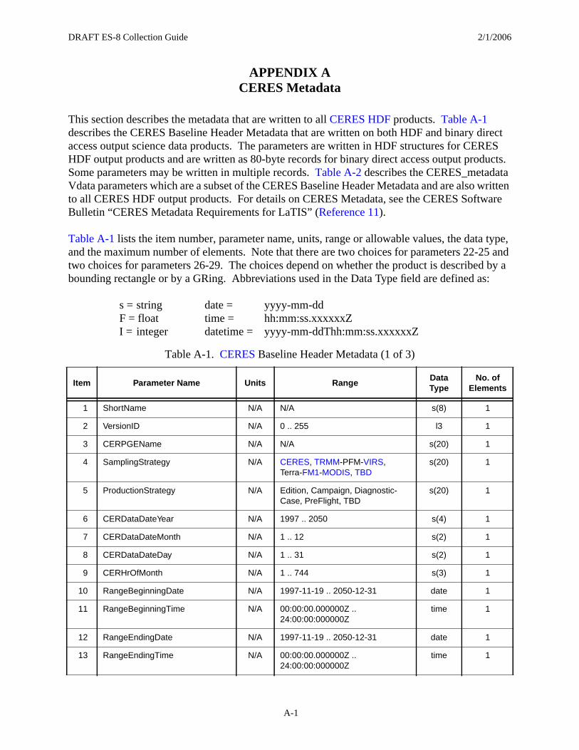
DRAFT ES-8 Collection Guide 2/1/2006
A-1
APPENDIX A CERES Metadata
This section describes the metadata that are written to all CERES HDF products. Table A-1 describes the CERES Baseline Header Metadata that are written on both HDF and binary direct access output science data products. The parameters are written in HDF structures for CERES HDF output products and are written as 80-byte records for binary direct access output products. Some parameters may be written in multiple records. Table A-2 describes the CERES_metadata Vdata parameters which are a subset of the CERES Baseline Header Metadata and are also written to all CERES HDF output products. For details on CERES Metadata, see the CERES Software Bulletin “CERES Metadata Requirements for LaTIS” (Reference 11).
Table A-1 lists the item number, parameter name, units, range or allowable values, the data type, and the maximum number of elements. Note that there are two choices for parameters 22-25 and two choices for parameters 26-29. The choices depend on whether the product is described by a bounding rectangle or by a GRing. Abbreviations used in the Data Type field are defined as:
s = string date = yyyy-mm-ddF = float time = hh:mm:ss.xxxxxxZI = integer datetime = yyyy-mm-ddThh:mm:ss.xxxxxxZ
Table A-1. CERES Baseline Header Metadata (1 of 3)
Item Parameter Name Units RangeData Type
No. of Elements
1 ShortName N/A N/A s(8) 1
2 VersionID N/A 0 .. 255 l3 1
3 CERPGEName N/A N/A s(20) 1
4 SamplingStrategy N/A CERES, TRMM-PFM-VIRS, Terra-FM1-MODIS, TBD
s(20) 1
5 ProductionStrategy N/A Edition, Campaign, Diagnostic-Case, PreFlight, TBD
s(20) 1
6 CERDataDateYear N/A 1997 .. 2050 s(4) 1
7 CERDataDateMonth N/A 1 .. 12 s(2) 1
8 CERDataDateDay N/A 1 .. 31 s(2) 1
9 CERHrOfMonth N/A 1 .. 744 s(3) 1
10 RangeBeginningDate N/A 1997-11-19 .. 2050-12-31 date 1
11 RangeBeginningTime N/A 00:00:00.000000Z .. 24:00:00:000000Z
time 1
12 RangeEndingDate N/A 1997-11-19 .. 2050-12-31 date 1
13 RangeEndingTime N/A 00:00:00.000000Z .. 24:00:00:000000Z
time 1
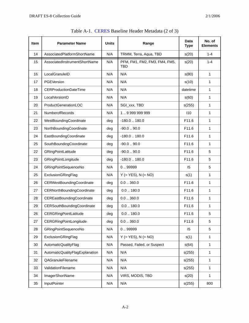
DRAFT ES-8 Collection Guide 2/1/2006
A-2
14 AssociatedPlatformShortName N/A TRMM, Terra, Aqua, TBD s(20) 1-4
15 AssociatedInstrumentShortName N/A PFM, FM1, FM2, FM3, FM4, FM5, TBD
s(20) 1-4
16 LocalGranuleID N/A N/A s(80) 1
17 PGEVersion N/A N/A s(10) 1
18 CERProductionDateTime N/A N/A datetime 1
19 LocalVersionID N/A N/A s(60) 1
20 ProductGenerationLOC N/A SGI_xxx, TBD s(255) 1
21 NumberofRecords N/A 1 .. 9 999 999 999 I10 1
22 WestBoundingCoordinate deg -180.0 .. 180.0 F11.6 1
23 NorthBoundingCoordinate deg -90.0 .. 90.0 F11.6 1
24 EastBoundingCoordinate deg -180.0 .. 180.0 F11.6 1
25 SouthBoundingCoordinate deg -90.0 .. 90.0 F11.6 1
22 GRingPointLatitude deg -90.0 .. 90.0 F11.6 5
23 GRingPointLongitude deg -180.0 .. 180.0 F11.6 5
24 GRingPointSequenceNo N/A 0 .. 99999 I5 5
25 ExclusionGRingFlag N/A Y (= YES), N (= NO) s(1) 1
26 CERWestBoundingCoordinate deg 0.0 .. 360.0 F11.6 1
27 CERNorthBoundingCoordinate deg 0.0 .. 180.0 F11.6 1
28 CEREastBoundingCoordinate deg 0.0 .. 360.0 F11.6 1
29 CERSouthBoundingCoordinate deg 0.0 .. 180.0 F11.6 1
26 CERGRingPointLatitude deg 0.0 .. 180.0 F11.6 5
27 CERGRingPointLongitude deg 0.0 .. 360.0 F11.6 5
28 GRingPointSequenceNo N/A 0 .. 99999 I5 5
29 ExclusionGRingFlag N/A Y (= YES), N (= NO) s(1) 1
30 AutomaticQualityFlag N/A Passed, Failed, or Suspect s(64) 1
31 AutomaticQualityFlagExplanation N/A N/A s(255) 1
32 QAGranuleFilename N/A N/A s(255) 1
33 ValidationFilename N/A N/A s(255) 1
34 ImagerShortName N/A VIRS, MODIS, TBD s(20) 1
35 InputPointer N/A N/A s(255) 800
Table A-1. CERES Baseline Header Metadata (2 of 3)
Item Parameter Name Units RangeData Type
No. of Elements
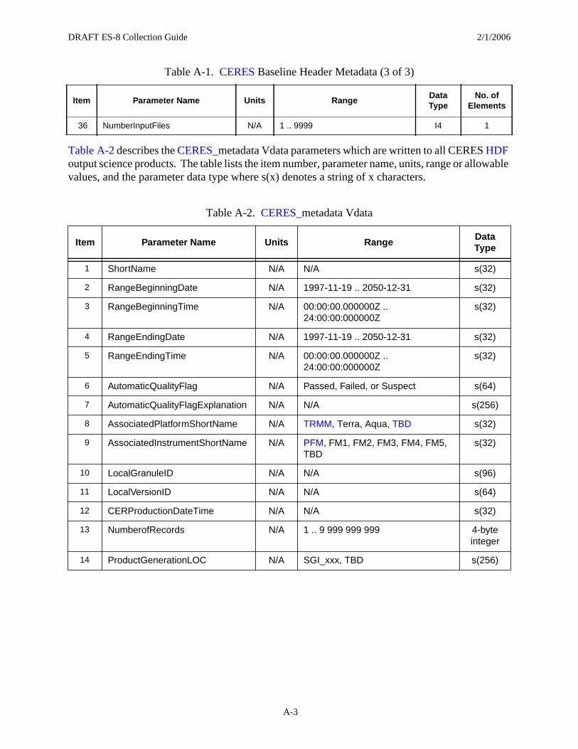
DRAFT ES-8 Collection Guide 2/1/2006
A-3
Table A-2 describes the CERES_metadata Vdata parameters which are written to all CERES HDF output science products. The table lists the item number, parameter name, units, range or allowable values, and the parameter data type where s(x) denotes a string of x characters.
36 NumberInputFiles N/A 1 .. 9999 I4 1
Table A-2. CERES_metadata Vdata
Item Parameter Name Units RangeData Type
1 ShortName N/A N/A s(32)
2 RangeBeginningDate N/A 1997-11-19 .. 2050-12-31 s(32)
3 RangeBeginningTime N/A 00:00:00.000000Z .. 24:00:00:000000Z
s(32)
4 RangeEndingDate N/A 1997-11-19 .. 2050-12-31 s(32)
5 RangeEndingTime N/A 00:00:00.000000Z .. 24:00:00:000000Z
s(32)
6 AutomaticQualityFlag N/A Passed, Failed, or Suspect s(64)
7 AutomaticQualityFlagExplanation N/A N/A s(256)
8 AssociatedPlatformShortName N/A TRMM, Terra, Aqua, TBD s(32)
9 AssociatedInstrumentShortName N/A PFM, FM1, FM2, FM3, FM4, FM5, TBD
s(32)
10 LocalGranuleID N/A N/A s(96)
11 LocalVersionID N/A N/A s(64)
12 CERProductionDateTime N/A N/A s(32)
13 NumberofRecords N/A 1 .. 9 999 999 999 4-byte integer
14 ProductGenerationLOC N/A SGI_xxx, TBD s(256)
Table A-1. CERES Baseline Header Metadata (3 of 3)
Item Parameter Name Units RangeData Type
No. of Elements