cls run fall 2017 logbook -...
TRANSCRIPT

CLS Run Fall 2017 Logbook
November 28 - December 1, 2017
Participants: Andrei Semenov, Nazanin Samadi, and Richard Jones Useful numbers: Richard Jones 860-377-5224
Table of Contents
Goals for this run 2
CLS Beam Permit document 4
Info from previous run 4
Shift schedule 5
Useful Information 5
Unpacking the diamonds 6
Mounting JD70-101 in beamline 6
Setup of data transfer to UConn 8
Initial scans 9
Rocking curves of JD70-101 9
Analysis of data from JD70-101 10
Dismounting of JD70-101 13
Study of JD70-103 14
Mounting JD70-103 in the target holder 14
Rocking curves of JD70-103 14
Analysis of data from JD70-103 14
Dismounting JD70-103 17
Study of JD70-106 18
Mounting JD70-106 in the target holder 18
Rocking curves of JD70-106 18
Analysis of data from JD70-106 18
1

Dismounting JD70-106 21
Study of JD70-107 22
Mounting JD70-107 in the target holder 22
Rocking curve setup procedure 22
Rocking curve analysis procedure 24
Rocking curves of JD70-107 26
Analysis of data from JD70-107 26
Dismounting JD70-107 29
Study of JD70-109 30
Rocking curves of JD70-109 30
Analysis of data from JD70-109 30
Dismounting JD70-109 33
Study of J1a-50 34
Mounting J1a-50 in the target holder 34
Rocking curves of J1a-50 37
Analysis of data from J1a-50 37
Dismounting J1a-50 40
Packing up and checking out 44
Goals for this run 1. Unpack the diamonds 2. Mount JD70-101 on holder and install in beamline 3. Check out beamline optics and verify camera focus 4. Take rocking curves of JD70-101 in 4 orientations 5. Transfer data from JD70-101 to UConn, verify data quality 6. Dismount JD70-101 and return to packaging 7. Mount JD70-103 on holder and install in beamline 8. Take rocking curves of JD70-103 in 4 orientations 9. Transfer data from JD70-103 to UConn, verify data quality 10. Dismount JD70-103 and return to packaging
2

11. Mount JD70-106 on holder and install in beamline 12. Take rocking curves of JD70-106 in 4 orientations 13. Transfer data from JD70-106 to UConn, verify data quality 14. Dismount JD70-106 and return to packaging 15. Mount JD70-107 on holder and install in beamline 16. Take rocking curves of JD70-107 in 4 orientations 17. Transfer data from JD70-107 to UConn, verify data quality 18. Dismount JD70-107 and return to packaging 19. Mount JD70-109 on holder and install in beamline 20. Take rocking curves of JD70-109 in 4 orientations 21. Transfer data from JD70-109 to UConn, verify data quality 22. Dismount JD70-109 and return to packaging 23. Mount J1a-50 on holder and install in beamline 24. Take rocking curves of J1a-50 in 4 orientations 25. Transfer data from J1a50-50 to UConn, verify data quality 26. Dismount J1a-50 and return to packaging 27. Transfer all remaining data, photos, and software tools to UConn 28. Clean up and check out
3
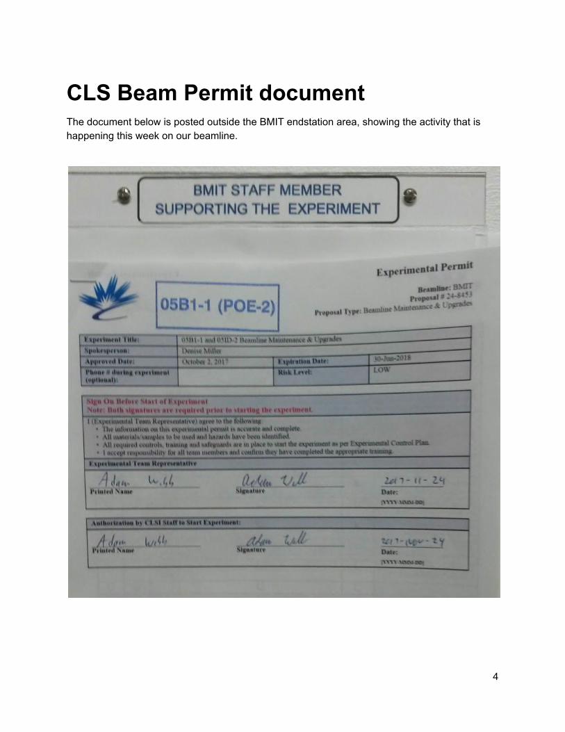
CLS Beam Permit document The document below is posted outside the BMIT endstation area, showing the activity that is happening this week on our beamline.
4

Info from previous run The logbooks from the August, 2016 run is a valuable store of useful information for how to carry out these rocking curve measurements at CLS. Use the link below to obtain read-only access.
● Logbook from GlueX CLS summer run 2016 ● Link to photos taken during summer run 2016 ● Logbook from CLS run in September, 2016 ● Link to photo directory from September, 2016
Shift schedule Useful Information
● Phone numbers a. Andrei Semenov, email: [email protected], cell: 306-502-5291 b. Richard Jones, email [email protected], cell: 860-377-5224 c. Adam Webb, BMIT Science Associate, office: 306-657-3846, cell: 306-372-8304 d. Nazanin Samadi, BMIT Technical Assistant, cell: 306-717-5469 e. BMIT and other CLS phone numbers: see image below
5

Unpacking the diamonds November 28, 2017 18:00 [rtj] I unwrapped the bubble wrap from around the diamond carrying case and tools. Everything looked normal visually, so I assume that they all survived the trip intact. Nazanin found a small Allen tool that I was able to use to tighten the small screws that hold the diamond on the mounting bar. We only have the bar with the tapped holes this time, not the ring that the bar mounted to during prior runs.
Mounting JD70-101 in beamline November 28, 19:00 First Nazanin used a molybdenum absorber in the beam to adjust the monochromator energy to put it right at 20.000 keV, within 1eV. Then we took out the moly absorber and centered our first test diamond JD70-101 in the beam. The horizontal slits were adjusted to make the beam spot just a bit larger than the target on either side. The vertical height of the beam is 8mm at this target position, just barely large enough to cover our 7mm diamonds. We used a fluorescent screen to make sure that the diamond is centered vertically within the beam.
JD70-101 diamond mounted on the beamline. This crystal location is for the scan #1.
6

The side view of the JD70-101 setup. The camera is mounted similar to that it was in the end of Summer 2016 run.
JD70-101 is in the foreground, but difficult to see in this image. The “1” on the aluminum tab identifies this diamond.
7

To help us find the reflections faster, Adam and Nazanin set up an old fashioned analog video camera for viewing the fluorescent screen while rotating the target. We were able to see the 2,2,0 reflection from JD70-101 very quickly using this method. It was only 0.3 degrees away from the dead-reckoning position that we set up with a protractor referencing the side of the mounting frame. After finding the reflection, we removed the fluorescent screen and took a few camera images of the reflected spot near the maximum of the Bragg intensity. In the bright central region of the diamond at the Bragg maximum, we are seeing camera pixels with numerical intensity between 1300 and 1800. This compares well with what I see for the sum hbase + hamp in JD70-100_00x_results.root from last year. So we are back to running conditions from fall 2016, and close to ready for production data taking. Nazanin cropped the camera acquisition region to an area of 1000 x 1000 pixels that is large enough to completely contain the diamond image. This cropping helps to reduce the total size of the dataset for a rocking curve scan, while retaining all of the useful data.
With the JD70-101 crystal set near the maximum of the Bragg curve, Nazanin tweaked the Hamamatsu focusing module and watched the sharpness of features in the updating camera image vary with the focus setting. Using those features, and the sharpness of the crystal edge she was able to find an optimum focus. It appears that the edge is only 2-3 pixels wide once the adjustments were made. Initially the resolution was visibly worse, so this is something that we need to keep an eye on, and include in the setup steps for all future runs. Beam size is 8mm vertical at the sample now, same as in the August run.
Setup of data transfer to UConn Next we configured the globus file transfer service for pushing rocking curve data to UConn. To do this, the following steps were needed.
1. Log in on the globus.org web interface. For this I use my GlobusID jonesrt and the password that is stored in my kkdb.
2. Review under “endpoints” the ones that are “administered by me”. This included one named jonesrt#grinch and one named BMIT-BM. The BMIT-BM was marked as disabled. I learned that the machine we were originally set up on in 2016 has been retired, so we needed to configure a new personal endpoint for the BMIT beamline PC.
a. do “setup a new personal endpoint” on the globusonline web gui, on the BMIT Windows pc WKS-w002587.
b. create a new UUID 98c71e94-d515-11e7-96c0-22000a8cbd7d, legacy name is jonesrt#98c71e94-d515-11e7-96c0-22000a8cbd7d
c. download and install the globusonline server package, needs admin privs d. during the software install, configure the shared folder under which export/import
of data is based. If this needs to be changed later, under the System Tray find the icon for the globusonline personal endpoint service, right click and choose options.
8
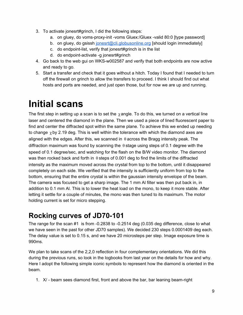
3. To activate jonesrt#grinch, I did the following steps: a. on gluey, do voms-proxy-init -voms Gluex:/Gluex -valid 80:0 [type password] b. on gluey, do gsissh [email protected] [should login immediately] c. do endpoint-list, verify that jonesrt#grinch is in the list d. do endpoint-activate -g jonesrt#grinch
4. Go back to the web gui on WKS-w002587 and verify that both endpoints are now active and ready to go.
5. Start a transfer and check that it goes without a hitch. Today I found that I needed to turn off the firewall on grinch to allow the transfers to proceed. I think I should find out what hosts and ports are needed, and just open those, but for now we are up and running.
Initial scans The first step in setting up a scan is to set the angle. To do this, we turned on a vertical lineχ laser and centered the diamond in the plane. Then we used a piece of lined fluorescent paper to find and center the diffracted spot within the same plane. To achieve this we ended up needing to change by 2.19 deg. This is well within the tolerance with which the diamond axes areχ aligned with the edges. After this, we scanned in across the Bragg intensity peak. Theθ diffraction maximum was found by scanning the stage using steps of 0.1 degree with theθ speed of 0.1 degree/sec, and watching for the flash on the B/W video monitor. The diamond was then rocked back and forth in steps of 0.001 deg to find the limits of the diffractedθ intensity as the maximum moved across the crystal from top to the bottom, until it disappeared completely on each side. We verified that the intensity is sufficiently uniform from top to the bottom, ensuring that the entire crystal is within the gaussian intensity envelope of the beam. The camera was focused to get a sharp image. The 1 mm Al filter was then put back in, in addition to 0.1 mm Al. This is to lower the heat load on the mono, to keep it more stable. After letting it settle for a couple of minutes, the mono was then tuned to its maximum. The motor holding current is set for micro stepping.
Rocking curves of JD70-101 The range for the scan #1 is from -0.2838 to -0.2514 deg (0.035 deg difference, close to what we have seen in the past for other JD70 samples). We decided 230 steps 0.0001409 deg each. The delay value is set to 0.15 s, and we have 20 microsteps per step. Image exposure time is 990ms.
We plan to take scans of the 2,2,0 reflection in four complementary orientations. We did this during the previous runs, so look in the logbooks from last year on the details for how and why. Here I adopt the following simple iconic symbols to represent how the diamond is oriented in the beam.
1. X/ - beam sees diamond first, front and above the bar, bar leaning beam-right
9
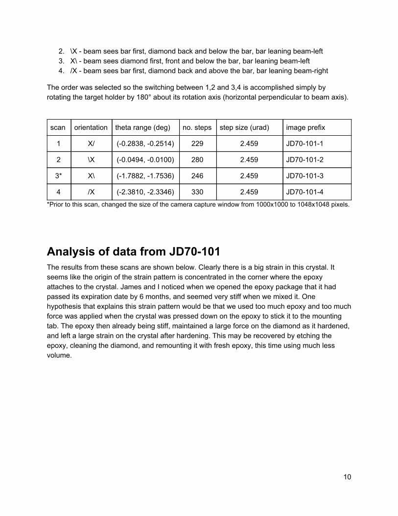
2. \X - beam sees bar first, diamond back and below the bar, bar leaning beam-left 3. X\ - beam sees diamond first, front and below the bar, bar leaning beam-left 4. /X - beam sees bar first, diamond back and above the bar, bar leaning beam-right
The order was selected so the switching between 1,2 and 3,4 is accomplished simply by rotating the target holder by 180° about its rotation axis (horizontal perpendicular to beam axis).
scan orientation theta range (deg) no. steps step size (urad) image prefix
1 X/ (-0.2838, -0.2514) 229 2.459 JD70-101-1
2 \X (-0.0494, -0.0100) 280 2.459 JD70-101-2
3* X\ (-1.7882, -1.7536) 246 2.459 JD70-101-3
4 /X (-2.3810, -2.3346) 330 2.459 JD70-101-4
*Prior to this scan, changed the size of the camera capture window from 1000x1000 to 1048x1048 pixels.
Analysis of data from JD70-101 The results from these scans are shown below. Clearly there is a big strain in this crystal. It seems like the origin of the strain pattern is concentrated in the corner where the epoxy attaches to the crystal. James and I noticed when we opened the epoxy package that it had passed its expiration date by 6 months, and seemed very stiff when we mixed it. One hypothesis that explains this strain pattern would be that we used too much epoxy and too much force was applied when the crystal was pressed down on the epoxy to stick it to the mounting tab. The epoxy then already being stiff, maintained a large force on the diamond as it hardened, and left a large strain on the crystal after hardening. This may be recovered by etching the epoxy, cleaning the diamond, and remounting it with fresh epoxy, this time using much less volume.
10

JD70-101 mean peak maps. The lower edge of the diamond is being cut off in scans 2 and 3 by the edge of the beam. For future scans, we will be more careful about the vertical alignment of the diamond in the beam, since the beam spot is really only 8mm high and the edges on the beam vertical intensity profile are very sharp..
11

JD70-101 sigma peak maps. There is noticeable broadening of the peaks in the places where excess epoxy flowed onto the surface of the diamond. However, the peak widths are really very good over most of the surface area.
12

JD70-101 whole-crystal rocking curves. The broadening seen in these plots makes this crystal unusable as it is.
Dismounting of JD70-101 I removed JD70-101 from the mounting bar and returned it to the plastic storage pod. When I did this, I made a visual inspection of the surface of the sample. There are clear non-planar features visible in the reflection from the crystal surfaces on both sides. However, I was unable to see anything in those reflected patterns that resembles the strain pattern seen in the X-rays. This is consistent with experience in the past: that these diamond are very stiff and the strain in the crystal geometry is too small to see by simply viewing the surface with visible light. The structure of the surface is dominated by irregularities imprinted on the surface during polishing, and does not reflect the underlying crystal strain.
13

Study of JD70-103
Mounting JD70-103 in the target holder The mounting bar was removed from the target holder when removing JD70-101. I then took JD70-103 from its pocket in the plastic transport pod and installed in on the middle of the bar. The crystal is clearly marked by a “3” written on the aluminum tab. We then installed the bar in position X/ in the target holder, doing our best to align it with the upper edge of the crystal in the horizontal plane.
Rocking curves of JD70-103
scan orientation theta range (deg) no. steps step size (urad) image prefix
1 X/ (-1.1802, -1.1417) 274 2.459 JD70-103-1
2* X/ (1.1010, 1.1346) 239 2.459 JD70-103-2
3 \X (0.2212, 0.2469) 182 2.459 JD70-103-3
4 X\ (-1.1061, -1.1456) 280 2.459 JD70-103-4
5 /X (-0.7479,-0.7104) 266 2.459 JD70-103-5
*Scan 2 repeats scan 1 with the diamond shifted upward to make up for lost intensity at the bottom.
Analysis of data from JD70-103 The rocking curve maps from JD70-103 are shown below.
14

JD70-103 mean peak maps. The upper edge of the diamond is being cut off in scans 2 and 5 by the edge of the beam. For future scans, we will be more careful about the vertical alignment of the diamond in the beam.
15

.
JD70-103 sigma peak maps. There is noticeable broadening of the peaks in the places where excess epoxy flowed onto the surface of the diamond. However, the peak widths are really very good over most of the surface area.
16

JD70-103 whole-crystal rocking curves. This crystal is much better than JD70-101, may be usable as-is if needed.
Dismounting JD70-103 We pulled the mounting bar out of the target holder and removed JD70-103 from the bar. Visually everything looks the same as when we mounted it. The JD70-103 crystal and tab are now back in the plastic transport pod, in the slot labeled JD70-103.
17

Study of JD70-106
Mounting JD70-106 in the target holder I took JD70-106 from its pocket in the plastic transport pod and installed in on the middle of the bar. The crystal is clearly marked by a “6” written on the aluminum tab. Andrei noticed that this crystal epoxied at an angle quite far from 45° with respect to the tab edge. We then installed the bar in position X/ in the target holder, doing our best to align it with the upper edge of the crystal in the horizontal plane.
Rocking curves of JD70-106
scan orientation theta range (deg) no. steps step size (urad) image prefix
1* X/ (-0.4113, -0.3136) 347 4.918 JD70-106-1
2 \X (-0.0959, 0.0066) 364 4.918 JD70-106-2
3 X\ (0.1559, 0.2486) 329 4.918 JD70-106-3
4 /X (0.4644, 0.6243) 567 4.918 JD70-106-4
* Scan range is very large for this crystal, so we doubled the step size to limit the duration of these scans.
Analysis of data from JD70-106 The rocking curve images from JD70-106 are shown below.
18

JD70-106 mean peak maps. The upper edge of the diamond is being cut off in scans 1 and 2 by the edge of the beam. For future scans, we will be more careful about the vertical alignment of the diamond in the beam.
19
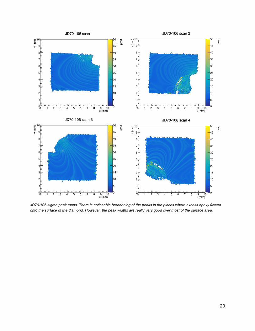
JD70-106 sigma peak maps. There is noticeable broadening of the peaks in the places where excess epoxy flowed onto the surface of the diamond. However, the peak widths are really very good over most of the surface area.
20

JD70-106 whole-crystal rocking curves. This crystal is much worse than the others we have examined so far.
Dismounting JD70-106 We pulled the mounting bar out of the target holder and removed JD70-106 from the bar. Visually everything looks the same as when we mounted it. The JD70-106 crystal and tab are now back in the plastic transport pod, in the slot labeled JD70-106.
21

Study of JD70-107
Mounting JD70-107 in the target holder I took JD70-107 from its pocket in the plastic transport pod and installed in on the middle of the bar. The crystal is clearly marked by a “7” written on the aluminum tab. We then installed the bar in position X/ in the target holder, doing our best to align it with the upper edge of the crystal in the horizontal plane.
Rocking curve setup procedure Here I document the repeatable procedures that we have gradually refined as we proceed through these measurements.
1. Enter the hutch. 2. Loosen the Allen screw on the right side of the target holder so it is free to rotate about
its rotation axis. Rotate to make the side with the pinch bars and nuts face upstream, and loosen the nuts.
3. Mount the diamond bar under the pinch bars in the target holder, in the designated orientation (eg. X/). Adjust the position of the diamond to center it in the target holder frame, at an angle that makes the edges of the diamond parallel to the frame edges.
4. Rotate the target holder so the diamond faces in the direction consistent with the designated orientation (eg. upstream for X/), and tighten the right Allen screw on the target holder. The left screw can be left slack to simplify future steps.
5. Use the horizontal and vertical alignment line lasers to check that the height of the diamond is approximately centered in the beam horizontally and vertically.
6. Place the fluorescent graph paper in front of the camera, with the vertical line that is marked in ink aligned with the vertical line laser stripe.
7. Close the hutch. Turn on the beam, verify that the hutch shutter is open. Verify that the fluorescent graph paper is visible in the video camera screen, and turn off the lights inside the hutch.
8. Zero all of the relative positions of the motors: in the target motion gui screens., θ, z, xχ 9. Do a search in to find the Bragg reflection. We found that it was best to start with aθ
search window (0,+1) followed by (0,-1) in degrees, motor speed 0.1deg/s. If it was not found there, we would enlarge the search window to cover (1,2) and (-1,-2) and continue until it was found. If not, we would question whether the diamond was off in height, adjust the height in the direction we suspect it might be off, and repeat the search.
10. If having difficulties seeing the reflection in step #9 above, we would sometimes remove the 1mm Al absorber. This takes a couple of minutes to take out and put in, so we would avoid doing this unless we were having trouble seeing the spot.
22
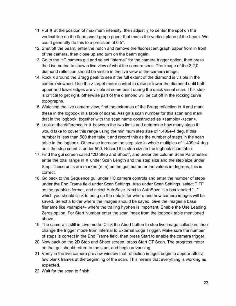
11. Put at the position of maximum intensity, then adjust to center the spot on theθ χ vertical line on the fluorescent graph paper that marks the vertical plane of the beam. We could generally do this to a precision of 0.5°.
12. Shut off the beam, enter the hutch and remove the fluorescent graph paper from in front of the camera, then close up and turn on the beam again.
13. Go to the HC camera gui and select “internal” for the camera trigger option, then press the Live button to show a live view of what the camera sees. The image of the 2,2,0 diamond reflection should be visible in the live view of the camera image.
14. Rock around the Bragg peak to see if the full extent of the diamond is visible in theθ camera viewport. Use the z target motor control to raise or lower the diamond until both upper and lower edges are visible at some point during the quick visual scan. This step is critical to get right, otherwise part of the diamond will be cut off in the rocking curve topographs.
15. Watching the live camera view, find the extremes of the Bragg reflection in and markθ these in the logbook in a table of scans. Assign a scan number for this scan and mark that in the logbook, together with the scan name constructed as <sample>-<scan>.
16. Look at the difference in between the two limits and determine how many steps itθ would take to cover this range using the minimum step size of 1.409e-4 deg. If this number is less than 500 then take it and record this as the number of steps in the scan table in the logbook. Otherwise increase the step size in whole multiples of 1.409e-4 deg until the step count is under 500. Record this step size in the logbook scan table.
17. Find the gui screen called “2D Step and Shoot”, and under the column Scan Parameters enter the total range in under Scan Length and the step size and the step size underθ Step. These units are marked (mm) on the gui, but enter the values in degrees, this is correct.
18. Go back to the Sequence gui under HC camera controls and enter the number of steps under the End Frame field under Scan Settings. Also under Scan Settings, select TIFF as the graphics format, and select AutoSave. Next to AutoSave is a box labeled “...” which you should click to bring up the details for where and how camera images will be saved. Select a folder where the images should be saved. Give the images a base filename like <sample>- where the trailing hyphen is important. Enable the Use Leading Zeros option. For Start Number enter the scan index from the logbook table mentioned above.
19. The camera is still in Live mode. Click the Abort button to stop live image collection, then change the trigger mode from Internal to External Edge Trigger. Make sure the number of steps is correct in the End Frame field, then press Start to enable the camera trigger.
20. Now back on the 2D Step and Shoot screen, press Start CT Scan. The progress meter on that gui should return to the start, and begin advancing.
21. Verify in the live camera preview window that reflection images begin to appear after a few blank frames at the beginning of the scan. This means that everything is working as expected.
22. Wait for the scan to finish.
23

Rocking curve analysis procedure 1. Use globus online to transfer the folder containing all of the images taken in the previous
scan to jonesrt#grinch. These data should land in grinch.phys.uconn.edu:/export/data0. 2. Create a data analysis area on /nfs/direct/jonesrt, eg. /nfs/direct/jonesrt/cls-11-2017 and
create a work directory for this sample, eg. /nfs/direct/jonesrt/cls-11-2017/JD70-101, then use rsync to copy image files from grinch to this work area. This separation between directories used for transfer and analysis is useful so that one can rename files in the analysis area without having them overwritten by the next globus transfer. This renaming happens whenever someone mistypes the image prefix or sequence numbering options during image acquisition, and lets the names be rewritten into canonical form before attempting to run the analysis. Canonical form for images is <sample>-<scan>_<N>.tif where step number N ranges from 1 to the number of steps and has leading zeros to make the total number of digits equal to 5.
3. Go to /home/www/docs/halld/diamonds on gluey.phys.uconn.edu and make a new directory for this run, eg. cls-11-2017. Inside this directory, create a symlink called “data” to the work area on /nfs/direct/jonesrt/<run> created in step 2 above. Make another folder next to “data” called “photos” where photographs from the run will be stored. Then cd into data and add a symlink back to /home/www/docs/halld/diamonds/Analysis called Analysis. Finally, from within Analysis, create a symlink to the same destination as /home/www/docs/halld/diamonds/<run>/data, and name it <run>. This completes the directory linkage structure assumed in the code and in these instructions.
4. Make a local copy of rcmaker.C (one can be found in the Analysis directory) in the sample directory under /home/www/docs/halld/diamonds/<run>/data/<sample>. Open a new terminal window and cd into this directory where the copy of rcmaker.C is found.
5. Start root in this window, and initialize the root session as follows: a. .L /usr/lib64/libtiff.so b. .L rcmaker.C+O
6. Each time a new scan is made and the data are pushed into the analysis area through globus + rsync steps, a new root command illustrated below must be issued to convert the raw image files into root histograms.
a. rcmaker(“<sample>”,<scan>,<steps>,1) 7. When this completes, use uberftp to push the output root file that contains all of the raw
data from this scan to pnfs. The file is named <sample>-<scan>_rocking_curves.root and should be found in the same directory as the tiff files that were used to create it. Ignore the warnings from the tiff conversion library about unexpected tags in the tiff header, as these do not cause any real problems. The destination directory on pnfs should be /pnfs/phys.uconn.edu/data/Gluex/beamline/diamonds/<run>/results. If this directory does not exist yet, it should be created and owned by the gluexuser user. Copying into this directory requires that the person doing the transfer have a valid voms proxy issued by the Gluex vo.
24

8. As soon as the X_rocking_curves.root file is uploaded to pnfs, the root process that fits the rocking curves to a gaussian peak over a constant background can be started. I use proof for this step, although if you are patient you can just run it in a regular root client session. The configuration of the proof service at UConn makes using this pretty straight-forward. Use the UConn-proof web interface to start your own private proof service, and then connect to that service to do your analysis. All of this is automated by the dofits.C script found in Analysis. The following session illustrates how to use it, from a root session started in the Analysis directory. Before you start this, edit the dofits.C file to make sure it points to your private proof service, and that the appropriate set of lines have been commented out so that only the scans that you want to fit are processed. All you need to do as the run progresses is just add a single line in the appropriate function within dofits.C for each scan you want to process, and comment them out as you finish each one.
a. .L Map2D.cc+O b. .L rcfitter.C+O c. .L rcpicker.C+O d. .L run_rcpicker.C+O e. .x dofits.C
9. The above step creates a new root output file <sample>-<scan>_results.root in the Analysis directory. Use uberftp to copy it to the same area on pnfs where you stored the X_rocking_curves.root file in one of the previous steps.
10. Edit the python script plotgen.py and follow the examples in the code to add a line to generate rocking curve topograph images for each scan with a X_results.root file that has been uploaded to pnfs, as described in the previous step. Run this file within a python session as follows.
a. import plotgen 11. Move the *.png files created in the last step into <run>/<sample>. Eventually at the end
of the run, you will back up these <sample> directories containing all of the raw image files into a compressed archive and then remove the tiff files, leaving behind only these png images. These are the final results from this analysis.
12. Delete the .root files created in the above steps after they have been copied into pnfs. This leaves behind a very small data footprint in the /home/www and /nfs/direct/jonesrt nfs areas, containing only a few png images and text files from each scan. The raw data and fitting results are stored in the root files that are archived on pnfs.
Keeping several terminal windows open on the screen, one for each of the steps above, is useful for being able to repeat similar commands each time a new scan comes in.
25
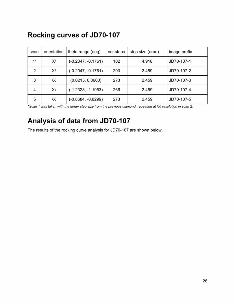
Rocking curves of JD70-107
scan orientation theta range (deg) no. steps step size (urad) image prefix
1* X/ (-0.2047, -0.1761) 102 4.918 JD70-107-1
2 X/ (-0.2047, -0.1761) 203 2.459 JD70-107-2
3 \X (0.0215, 0.0600) 273 2.459 JD70-107-3
4 X\ (-1.2328, -1.1953) 266 2.459 JD70-107-4
5 /X (-0.8684, -0.8299) 273 2.459 JD70-107-5 *Scan 1 was taken with the larger step size from the previous diamond, repeating at full resolution in scan 2.
Analysis of data from JD70-107 The results of the rocking curve analysis for JD70-107 are shown below.
26

JD70-107 mean peak maps. The central region looks pretty flat in these views, but the scan range is very large.
27

JD70-107 sigma peak maps. There is noticeable broadening of the peaks in the places where excess epoxy flowed onto the surface of the diamond. However, the peak widths are really very good over most of the surface area.
28

JD70-107 whole-crystal rocking curves. This crystal is not the worst one in this set, but it does not meet the requirements for GlueX. radiators.
Dismounting JD70-107 We pulled the mounting bar out of the target holder and removed JD70-107 from the bar. Visually everything looks the same as when we mounted it. The JD70-107 crystal and tab are now back in the plastic transport pod, in the slot labeled JD70-107.
29

Study of JD70-109 I took JD70-109 from its pocket in the plastic transport pod and installed in on the middle of the bar. The crystal is clearly marked by a “9” written on the aluminum tab. We then installed the bar in position X/ in the target holder, doing our best to align it with the upper edge of the crystal in the horizontal plane. This diamond appears to be tilted slightly out of the plane of the mounting tab. We may need to enlarge the search zone for the Bragg angle in aligning this diamond.
Rocking curves of JD70-109
scan orientation theta range (deg) no. steps step size (urad) image prefix
1 X/ (-2.8754, -2.7432) 469 4.818 JD70-109-1
2 \X (-2.5146, -2.3814) 473 4.818 JD70-109-2
3 X\ (-3.3574, -3.2173) 497 4.818 JD70-109-3
4 /X (-3.2226, -3.0874) 480 4.818 JD70-109-4
Analysis of data from JD70-109 The results of the rocking curve analysis for JD70-109 are shown below.
30
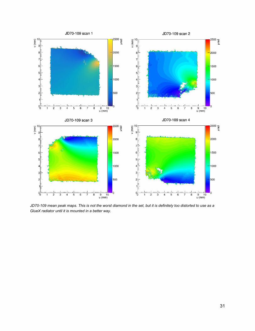
JD70-109 mean peak maps. This is not the worst diamond in the set, but it is definitely too distorted to use as a GlueX radiator until it is mounted in a better way.
31

.
JD70-109 sigma peak maps. There is noticeable broadening of the peaks in the places where excess epoxy flowed onto the surface of the diamond. However, the peak widths are really very good over most of the surface area.
32

JD70-109 whole-crystal rocking curves. This crystal is one of the worst in this set, if not the worst, in terms of whole crystal rocking curve width.
Dismounting JD70-109 We pulled the mounting bar out of the target holder and removed JD70-109 from the bar. Visually everything looks the same as when we mounted it. The JD70-109 crystal and tab are now back in the plastic transport pod, in the slot labeled JD70-109.
33

Study of J1a-50
Mounting J1a-50 in the target holder I took J1a-50 from its plastic protector inside the gem box it was transported in and installed in on the middle of the bar. The sample is clearly marked with “J1A50” written on the aluminum tab. We then installed the bar in position X/ in the target holder, doing our best to align it with the upper edge of the crystal in the horizontal plane.
34

35

36
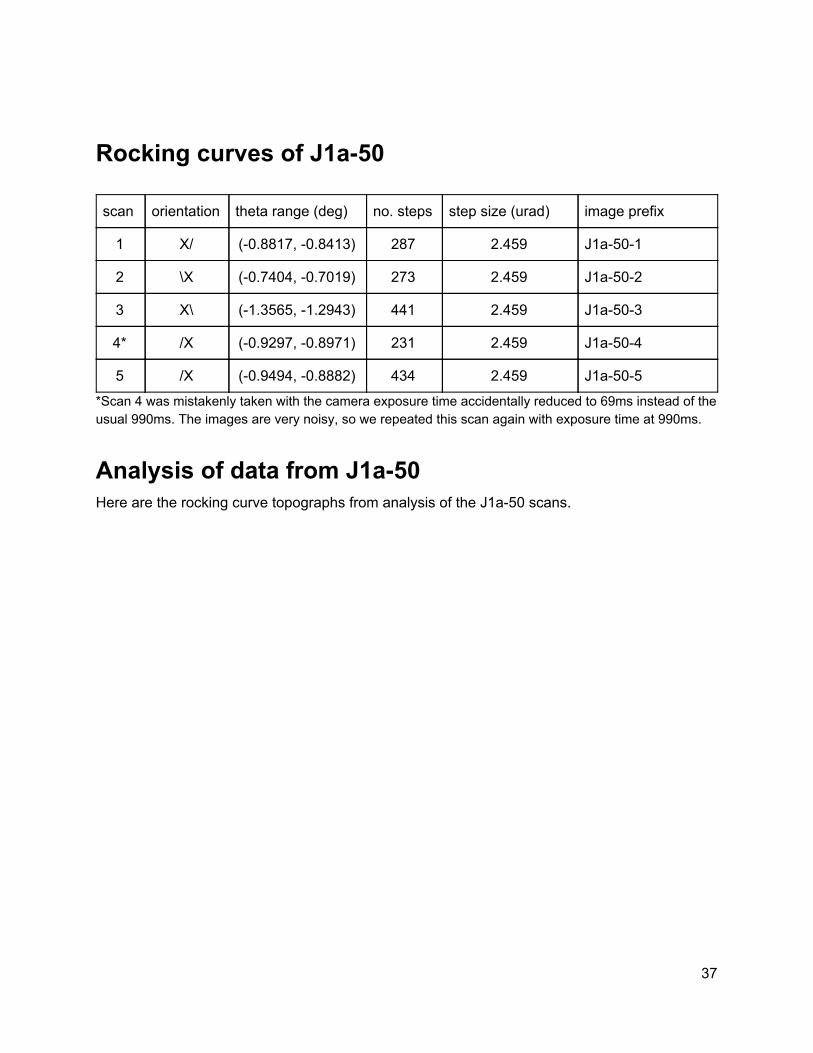
Rocking curves of J1a-50
scan orientation theta range (deg) no. steps step size (urad) image prefix
1 X/ (-0.8817, -0.8413) 287 2.459 J1a-50-1
2 \X (-0.7404, -0.7019) 273 2.459 J1a-50-2
3 X\ (-1.3565, -1.2943) 441 2.459 J1a-50-3
4* /X (-0.9297, -0.8971) 231 2.459 J1a-50-4
5 /X (-0.9494, -0.8882) 434 2.459 J1a-50-5
*Scan 4 was mistakenly taken with the camera exposure time accidentally reduced to 69ms instead of the usual 990ms. The images are very noisy, so we repeated this scan again with exposure time at 990ms.
Analysis of data from J1a-50 Here are the rocking curve topographs from analysis of the J1a-50 scans.
37

J1a-50 mean peak maps.
38

J1a-50 sigma peak maps.
39
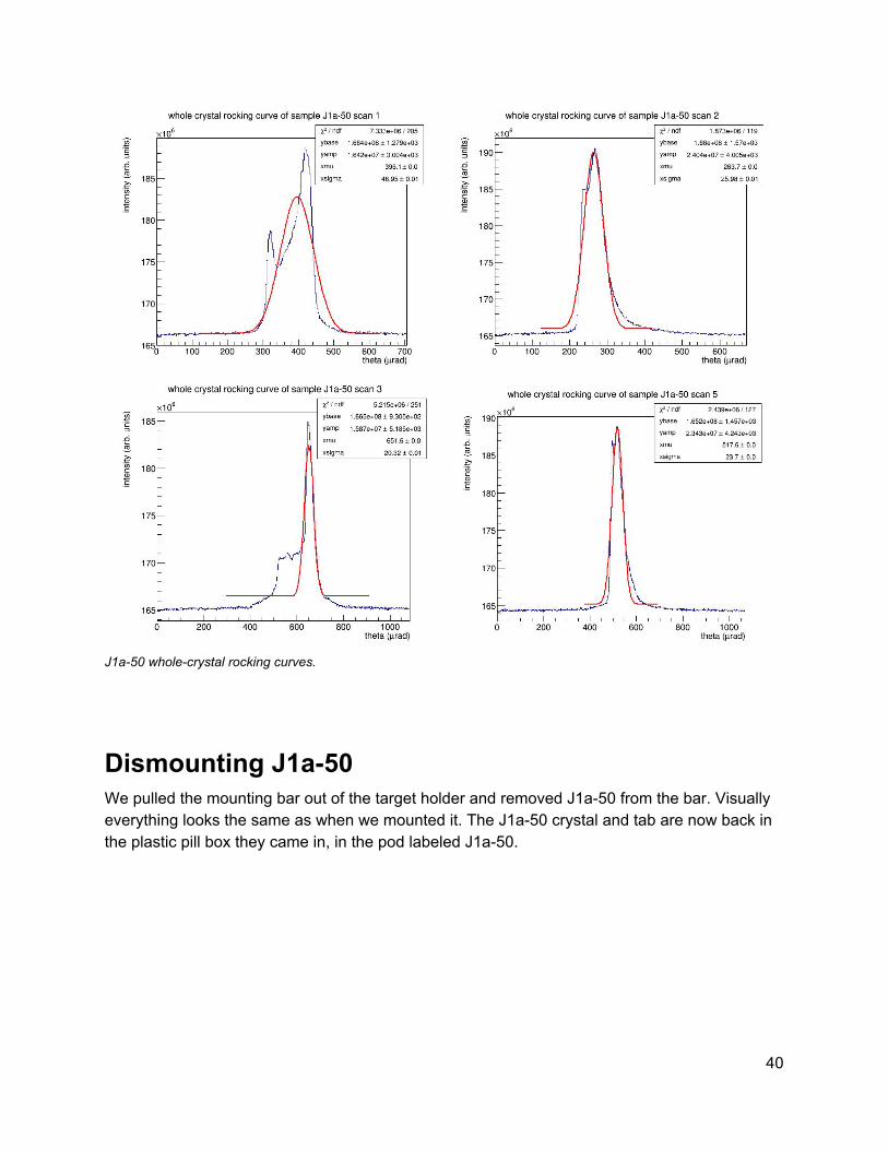
J1a-50 whole-crystal rocking curves.
Dismounting J1a-50 We pulled the mounting bar out of the target holder and removed J1a-50 from the bar. Visually everything looks the same as when we mounted it. The J1a-50 crystal and tab are now back in the plastic pill box they came in, in the pod labeled J1a-50.
40

41

42

43

Packing up and checking out
Goodbye, Saskatoon! It was a successful run, and great working with you all.
-Richard Jones
44