cluster analysis overview data mining techniques ...€“as a preprocessing step for other...

1

Data Mining Techniques: Cluster Analysis

Mirek Riedewald

Many slides based on presentations by Han/Kamber, Tan/Steinbach/Kumar, and Andrew

Moore

Cluster Analysis Overview

• Introduction

• Foundations: Measuring Distance (Similarity)

• Partitioning Methods: K-Means

• Hierarchical Methods

• Density-Based Methods

• Clustering High-Dimensional Data

• Cluster Evaluation

2

What is Cluster Analysis?

• Cluster: a collection of data objects – Similar to one another within the same cluster

– Dissimilar to the objects in other clusters

• Unsupervised learning: usually no training set with known “classes”

• Typical applications – As a stand-alone tool to get insight into data

properties

– As a preprocessing step for other algorithms

3

What is Cluster Analysis?

4

Inter-cluster

distances are maximized

Intra-cluster

distances are minimized

Rich Applications, Multidisciplinary Efforts

• Pattern Recognition

• Spatial Data Analysis

• Image Processing

• Data Reduction

• Economic Science – Market research

• WWW – Document classification

– Weblogs: discover groups of similar access patterns

5

Clustering precipitation in Australia

Examples of Clustering Applications

• Marketing: Help marketers discover distinct groups in their customer bases, and then use this knowledge to develop targeted marketing programs

• Land use: Identification of areas of similar land use in an earth observation database

• Insurance: Identifying groups of motor insurance policy holders with a high average claim cost

• City-planning: Identifying groups of houses according to their house type, value, and geographical location

• Earth-quake studies: Observed earth quake epicenters should be clustered along continent faults

6

2

Quality: What Is Good Clustering?

• Cluster membership objects in same class

• High intra-class similarity, low inter-class similarity

– Choice of similarity measure is important

• Ability to discover some or all of the hidden patterns

– Difficult to measure without ground truth

7

Notion of a Cluster can be Ambiguous

8

How many clusters?

Four Clusters Two Clusters

Six Clusters

Distinctions Between Sets of Clusters

• Exclusive versus non-exclusive – Non-exclusive clustering: points may belong to

multiple clusters

• Fuzzy versus non-fuzzy – Fuzzy clustering: a point belongs to every cluster with

some weight between 0 and 1 • Weights must sum to 1

• Partial versus complete – Cluster some or all of the data

• Heterogeneous versus homogeneous – Clusters of widely different sizes, shapes, densities

9


• Introduction







10

Distance

• Clustering is inherently connected to question of (dis-)similarity of objects

• How can we define similarity between objects?

11

Similarity Between Objects

• Usually measured by some notion of distance

• Popular choice: Minkowski distance

– q is a positive integer

• q = 1: Manhattan distance

• q = 2: Euclidean distance:

12

q qj

dxi

dx

qjxix

qjxixji |)()(||)(

2)(

2||)(

1)(

1|)(),(dist xx

|)()(||)(2

)(2

||)(1

)(1

|)(),(dist jd

xid

xjxixjxixji xx

2 2|)()(|2|)(2

)(2

|2|)(1

)(1

|)(),(dist jd

xid

xjxixjxixji xx

3

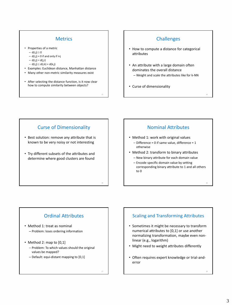
Metrics

• Properties of a metric – d(i,j) 0

– d(i,j) = 0 if and only if i=j

– d(i,j) = d(j,i)

– d(i,j) d(i,k) + d(k,j)

• Examples: Euclidean distance, Manhattan distance

• Many other non-metric similarity measures exist

• After selecting the distance function, is it now clear how to compute similarity between objects?

13

Challenges

• How to compute a distance for categorical attributes

• An attribute with a large domain often dominates the overall distance

– Weight and scale the attributes like for k-NN

• Curse of dimensionality

14

Curse of Dimensionality

• Best solution: remove any attribute that is known to be very noisy or not interesting

• Try different subsets of the attributes and determine where good clusters are found

15

Nominal Attributes

• Method 1: work with original values

– Difference = 0 if same value, difference = 1 otherwise

• Method 2: transform to binary attributes

– New binary attribute for each domain value

– Encode specific domain value by setting corresponding binary attribute to 1 and all others to 0

16

Ordinal Attributes

• Method 1: treat as nominal

– Problem: loses ordering information

• Method 2: map to [0,1]

– Problem: To which values should the original values be mapped?

– Default: equi-distant mapping to [0,1]

17

Scaling and Transforming Attributes

• Sometimes it might be necessary to transform numerical attributes to [0,1] or use another normalizing transformation, maybe even non-linear (e.g., logarithm)

• Might need to weight attributes differently

• Often requires expert knowledge or trial-and-error

18

4

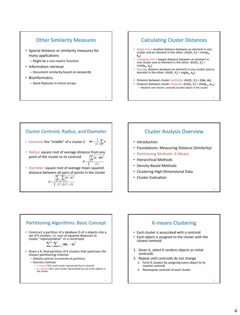
Other Similarity Measures

• Special distance or similarity measures for many applications

– Might be a non-metric function

• Information retrieval

– Document similarity based on keywords

• Bioinformatics

– Gene features in micro-arrays

19

Calculating Cluster Distances

• Single link = smallest distance between an element in one cluster and an element in the other: dist(Ki, Kj) = min(xip, xjq)

• Complete link = largest distance between an element in one cluster and an element in the other: dist(Ki, Kj) = max(xip, xjq)

• Average distance between an element in one cluster and an element in the other: dist(Ki, Kj) = avg(xip, xjq)

• Distance between cluster centroids: dist(Ki, Kj) = d(mi, mj) • Distance between cluster medoids: dist(Ki, Kj) = dist(xmi, xmj)

– Medoid: one chosen, centrally located object in the cluster

20

Cluster Centroid, Radius, and Diameter

• Centroid: the “middle” of a cluster C

• Radius: square root of average distance from any point of the cluster to its centroid

• Diameter: square root of average mean squared distance between all pairs of points in the cluster

21

CC x

xm||

1

||

)( 2

CR C

x

mx

)1|(|||

)(,

2

CCD

C Cx xyy

yx


• Introduction







22

Partitioning Algorithms: Basic Concept

• Construct a partition of a database D of n objects into a set of K clusters, s.t. sum of squared distances to cluster “representative” m is minimized

• Given a K, find partition of K clusters that optimizes the chosen partitioning criterion – Globally optimal: enumerate all partitions – Heuristic methods

• K-means (’67): each cluster represented by its centroid • K-medoids (’87): each cluster represented by one of the objects in

the cluster

23

K

i C ii1

2)(

xxm

K-means Clustering

• Each cluster is associated with a centroid • Each object is assigned to the cluster with the

closest centroid

1. Given K, select K random objects as initial centroids

2. Repeat until centroids do not change 1. Form K clusters by assigning every object to its

nearest centroid 2. Recompute centroid of each cluster

24

5

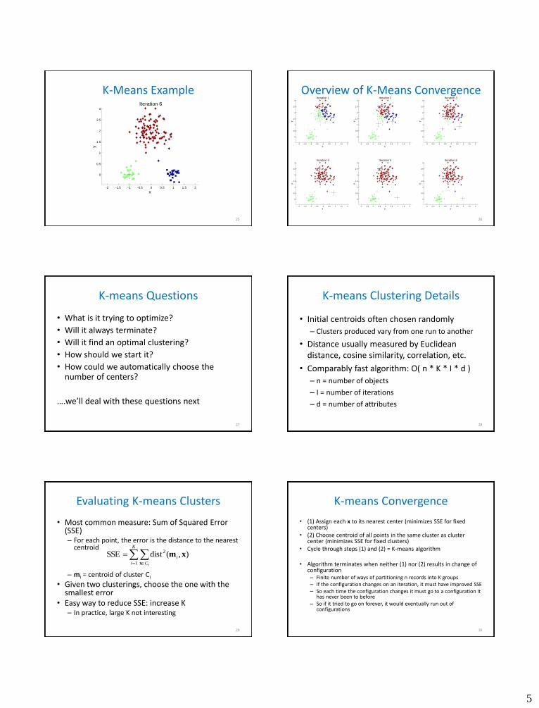
K-Means Example

25

-2 -1.5 -1 -0.5 0 0.5 1 1.5 2

0

0.5

1

1.5

2

2.5

3

x

y

Iteration 1

-2 -1.5 -1 -0.5 0 0.5 1 1.5 2

0

0.5

1

1.5

2

2.5

3

x

y

Iteration 2

-2 -1.5 -1 -0.5 0 0.5 1 1.5 2

0

0.5

1

1.5

2

2.5

3

x

y

Iteration 3

-2 -1.5 -1 -0.5 0 0.5 1 1.5 2

0

0.5

1

1.5

2

2.5

3

x

y

Iteration 4

-2 -1.5 -1 -0.5 0 0.5 1 1.5 2

0

0.5

1

1.5

2

2.5

3

x

y

Iteration 5

-2 -1.5 -1 -0.5 0 0.5 1 1.5 2

0

0.5

1

1.5

2

2.5

3

x

y

Iteration 6

Overview of K-Means Convergence

26

-2 -1.5 -1 -0.5 0 0.5 1 1.5 2

0

0.5

1

1.5

2

2.5

3

x

y

Iteration 1

-2 -1.5 -1 -0.5 0 0.5 1 1.5 2

0

0.5

1

1.5

2

2.5

3

x

y

Iteration 2

-2 -1.5 -1 -0.5 0 0.5 1 1.5 2

0

0.5

1

1.5

2

2.5

3

x

y

Iteration 3

-2 -1.5 -1 -0.5 0 0.5 1 1.5 2

0

0.5

1

1.5

2

2.5

3

x

y

Iteration 4

-2 -1.5 -1 -0.5 0 0.5 1 1.5 2

0

0.5

1

1.5

2

2.5

3

x

y

Iteration 5

-2 -1.5 -1 -0.5 0 0.5 1 1.5 2

0

0.5

1

1.5

2

2.5

3

x

y

Iteration 6

K-means Questions

• What is it trying to optimize?

• Will it always terminate?

• Will it find an optimal clustering?

• How should we start it?

• How could we automatically choose the number of centers?

….we’ll deal with these questions next

27

K-means Clustering Details

• Initial centroids often chosen randomly

– Clusters produced vary from one run to another

• Distance usually measured by Euclidean distance, cosine similarity, correlation, etc.

• Comparably fast algorithm: O( n * K * I * d )

– n = number of objects

– I = number of iterations

– d = number of attributes

28

Evaluating K-means Clusters

• Most common measure: Sum of Squared Error (SSE) – For each point, the error is the distance to the nearest

centroid

– mi = centroid of cluster Ci

• Given two clusterings, choose the one with the smallest error

• Easy way to reduce SSE: increase K – In practice, large K not interesting

29

K

i C

i

i1

2 ),(distSSEx

xm

K-means Convergence

• (1) Assign each x to its nearest center (minimizes SSE for fixed centers)

• (2) Choose centroid of all points in the same cluster as cluster center (minimizes SSE for fixed clusters)

• Cycle through steps (1) and (2) = K-means algorithm

• Algorithm terminates when neither (1) nor (2) results in change of configuration – Finite number of ways of partitioning n records into K groups – If the configuration changes on an iteration, it must have improved SSE – So each time the configuration changes it must go to a configuration it

has never been to before – So if it tried to go on forever, it would eventually run out of

configurations

30

6

Will it Find the Optimal Clustering?

31

-2 -1.5 -1 -0.5 0 0.5 1 1.5 2

0

0.5

1

1.5

2

2.5

3

x

y

-2 -1.5 -1 -0.5 0 0.5 1 1.5 2

0

0.5

1

1.5

2

2.5

3

x

y

Sub-optimal Clustering

-2 -1.5 -1 -0.5 0 0.5 1 1.5 2

0

0.5

1

1.5

2

2.5

3

x

y

Optimal Clustering

Original Points

Importance of Initial Centroids

32

-2 -1.5 -1 -0.5 0 0.5 1 1.5 2

0

0.5

1

1.5

2

2.5

3

x

y

Iteration 1

-2 -1.5 -1 -0.5 0 0.5 1 1.5 2

0

0.5

1

1.5

2

2.5

3

x

y

Iteration 2

-2 -1.5 -1 -0.5 0 0.5 1 1.5 2

0

0.5

1

1.5

2

2.5

3

x

y

Iteration 3

-2 -1.5 -1 -0.5 0 0.5 1 1.5 2

0

0.5

1

1.5

2

2.5

3

x

y

Iteration 4

-2 -1.5 -1 -0.5 0 0.5 1 1.5 2

0

0.5

1

1.5

2

2.5

3

x

y

Iteration 5

-2 -1.5 -1 -0.5 0 0.5 1 1.5 2

0

0.5

1

1.5

2

2.5

3

x

y

Iteration 6

Will It Find The Optimal Clustering Now?

33

-2 -1.5 -1 -0.5 0 0.5 1 1.5 2

0

0.5

1

1.5

2

2.5

3

x

y

Iteration 1

-2 -1.5 -1 -0.5 0 0.5 1 1.5 2

0

0.5

1

1.5

2

2.5

3

x

y

Iteration 2

-2 -1.5 -1 -0.5 0 0.5 1 1.5 2

0

0.5

1

1.5

2

2.5

3

x

y

Iteration 3

-2 -1.5 -1 -0.5 0 0.5 1 1.5 2

0

0.5

1

1.5

2

2.5

3

x

y

Iteration 4

-2 -1.5 -1 -0.5 0 0.5 1 1.5 2

0

0.5

1

1.5

2

2.5

3

x

y

Iteration 5

Importance of Initial Centroids

34

-2 -1.5 -1 -0.5 0 0.5 1 1.5 2

0

0.5

1

1.5

2

2.5

3

x

y

Iteration 1

-2 -1.5 -1 -0.5 0 0.5 1 1.5 2

0

0.5

1

1.5

2

2.5

3

x

y

Iteration 2

-2 -1.5 -1 -0.5 0 0.5 1 1.5 2

0

0.5

1

1.5

2

2.5

3

x

y

Iteration 3

-2 -1.5 -1 -0.5 0 0.5 1 1.5 2

0

0.5

1

1.5

2

2.5

3

x

y

Iteration 4

-2 -1.5 -1 -0.5 0 0.5 1 1.5 2

0

0.5

1

1.5

2

2.5

3

x

y

Iteration 5

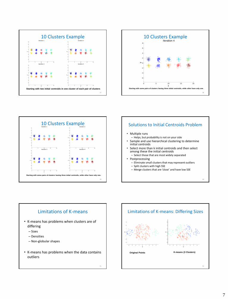
Problems with Selecting Initial Centroids

• Probability of starting with exactly one initial centroid per ‘real’ cluster is very low

– K selected for algorithm might be different from inherent K of the data

– Might randomly select multiple initial objects from same cluster

• Sometimes initial centroids will readjust themselves in the ‘right’ way, and sometimes they don’t

35

10 Clusters Example

36

0 5 10 15 20

-6

-4

-2

0

2

4

6

8

x

y

Iteration 1

0 5 10 15 20

-6

-4

-2

0

2

4

6

8

x

y

Iteration 2

0 5 10 15 20

-6

-4

-2

0

2

4

6

8

x

y

Iteration 3

0 5 10 15 20

-6

-4

-2

0

2

4

6

8

x

y

Iteration 4

Starting with two initial centroids in one cluster of each pair of clusters

7

10 Clusters Example

37

0 5 10 15 20

-6

-4

-2

0

2

4

6

8

x

y

Iteration 1

0 5 10 15 20

-6

-4

-2

0

2

4

6

8

x

y

Iteration 2

0 5 10 15 20

-6

-4

-2

0

2

4

6

8

x

y

Iteration 3

0 5 10 15 20

-6

-4

-2

0

2

4

6

8

x

y

Iteration 4

Starting with two initial centroids in one cluster of each pair of clusters

10 Clusters Example

38

Starting with some pairs of clusters having three initial centroids, while other have only one.

0 5 10 15 20

-6

-4

-2

0

2

4

6

8

x

y

Iteration 1

0 5 10 15 20

-6

-4

-2

0

2

4

6

8

x

y

Iteration 2

0 5 10 15 20

-6

-4

-2

0

2

4

6

8

x

y

Iteration 3

0 5 10 15 20

-6

-4

-2

0

2

4

6

8

x

y

Iteration 4

10 Clusters Example

39

Starting with some pairs of clusters having three initial centroids, while other have only one.

0 5 10 15 20

-6

-4

-2

0

2

4

6

8

x

y

Iteration 1

0 5 10 15 20

-6

-4

-2

0

2

4

6

8

x

y

Iteration 2

0 5 10 15 20

-6

-4

-2

0

2

4

6

8

x

y

Iteration 3

0 5 10 15 20

-6

-4

-2

0

2

4

6

8

x

y

Iteration 4

Solutions to Initial Centroids Problem

• Multiple runs – Helps, but probability is not on your side

• Sample and use hierarchical clustering to determine initial centroids

• Select more than k initial centroids and then select among these the initial centroids – Select those that are most widely separated

• Postprocessing – Eliminate small clusters that may represent outliers – Split clusters with high SSE – Merge clusters that are ‘close’ and have low SSE

40

Limitations of K-means

• K-means has problems when clusters are of differing

– Sizes

– Densities

– Non-globular shapes

• K-means has problems when the data contains outliers

41

Limitations of K-means: Differing Sizes

42

Original Points K-means (3 Clusters)

8

Limitations of K-means: Differing Density

43


Limitations of K-means: Non-globular Shapes

44


Overcoming K-means Limitations

45

Original Points K-means Clusters

One solution is to use many clusters.

Find parts of clusters, then put them together.


46



47


K-Means and Outliers

• K-means algorithm is sensitive to outliers – Centroid is average of cluster members

– Outlier can dominate average computation

• Solution: K-medoids – Medoid = most centrally located real object in a

cluster

– Algorithm similar to K-means, but finding medoid is much more expensive • Try all objects in cluster to find the one that minimizes SSE,

or just try a few randomly to reduce cost

48

9


• Introduction







49

Hierarchical Clustering

• Produces a set of nested clusters organized as a hierarchical tree

• Visualized as a dendrogram – Tree-like diagram that records the sequences of

merges or splits

50

1 3 2 5 4 60

0.05

0.1

0.15

0.2

1

2

3

4

5

6

1

23 4

5

Strengths of Hierarchical Clustering

• Do not have to assume any particular number of clusters

– Any number of clusters can be obtained by ‘cutting’ the dendogram at the proper level

• May correspond to meaningful taxonomies

– Example in biological sciences (e.g., animal kingdom, phylogeny reconstruction, …)

51

Hierarchical Clustering

• Two main types of hierarchical clustering

– Agglomerative:

• Start with the given objects as individual clusters

• At each step, merge the closest pair of clusters until only one cluster (or K clusters) left

– Divisive:

• Start with one, all-inclusive cluster

• At each step, split a cluster until each cluster contains a single object (or there are K clusters)

52

Agglomerative Clustering Algorithm

• More popular hierarchical clustering technique • Basic algorithm is straightforward

1. Compute the proximity matrix 2. Let each data object be a cluster 3. Repeat until only a single cluster remains

1. Merge the two closest clusters 2. Update the proximity matrix

• Key operation: computation of the proximity of two clusters – Different approaches to defining the distance

between clusters distinguish the different algorithms

53

Starting Situation

• Clusters of individual objects, proximity matrix

54

...p1 p2 p3 p4 p9 p10 p11 p12

p1

p3

p5

p4

p2

p1 p2 p3 p4 p5 . . .

.

.

. Proximity Matrix

10

Intermediate Situation

• Some clusters are merged

55

...p1 p2 p3 p4 p9 p10 p11 p12

C1

C4

C2 C5

C3

C2 C1

C1

C3

C5

C4

C2

C3 C4 C5

Proximity Matrix

Intermediate Situation

• Merge closest clusters (C2 and C5) and update proximity matrix

56

...p1 p2 p3 p4 p9 p10 p11 p12

C1

C4

C2 C5

C3

C2 C1

C1

C3

C5

C4

C2

C3 C4 C5

Proximity Matrix

After Merging

• How do we update the proximity matrix?

57

...p1 p2 p3 p4 p9 p10 p11 p12

C1

C4

C2 U C5

C3

? ? ? ?

?

?

?

C2

U

C5 C1

C1

C3

C4

C2 U C5

C3 C4

Proximity Matrix

Defining Cluster Distance

• Min: clusters near each other

• Max: low diameter

• Avg: more robust against outliers

• Distance between centroids

58

Strength of MIN

59

Original Points Two Clusters

• Can handle non-elliptical shapes

Limitations of MIN

60


• Sensitive to noise and outliers

11

Strength of MAX

61


• Less susceptible to noise and outliers

Limitations of MAX

62


•Tends to break large clusters

•Biased towards globular clusters

Hierarchical Clustering: Average

• Compromise between Single and Complete Link

• Strengths

– Less susceptible to noise and outliers

• Limitations

– Biased towards globular clusters

63

Cluster Similarity: Ward’s Method

• Distance of two clusters is based on the increase in squared error when two clusters are merged – Similar to group average if distance between

objects is distance squared

• Less susceptible to noise and outliers

• Biased towards globular clusters

• Hierarchical analogue of K-means – Can be used to initialize K-means

64

Hierarchical Clustering: Comparison

65

Group Average

Ward’s Method

1

2

3

4

5

6 1

2

5

3

4

MIN MAX

1

2

3

4

5

6

1

2

5

3 4

1

2

3

4

5

6

1

2 5

3

4 1

2

3

4

5

6

1

2

3

4

5

Time and Space Requirements

• O(n2) space for proximity matrix

– n = number of objects

• O(n3) time in many cases

– There are n steps and at each step the proximity matrix must be updated and searched

– Complexity can be reduced to O(n2 log(n) ) time for some approaches

66

12

Hierarchical Clustering: Problems and Limitations

• Once a decision is made to combine two clusters, it cannot be undone

• No objective function is directly minimized

• Different schemes have problems with one or more of the following: – Sensitivity to noise and outliers

– Difficulty handling different sized clusters and convex shapes

– Breaking large clusters

67


• Introduction







74

Density-Based Clustering Methods

• Clustering based on density of data objects in a neighborhood

– Local clustering criterion

• Major features:

– Discover clusters of arbitrary shape

– Handle noise

– Need density parameters as termination condition

75

DBSCAN: Basic Concepts

• Two parameters: – Eps: Maximum radius of the neighborhood

• NEps(q): {p D | dist(q,p) Eps}

– MinPts: Minimum number of points in an Eps-neighborhood of that point

• A point p is directly density-reachable from a point q w.r.t. Eps and MinPts if – p belongs to NEps(q)

– Core point condition: |NEps(q)| MinPts

76

p

q

MinPts = 5

Density-Reachable, Density-Connected

• A point p is density-reachable from a point q w.r.t. Eps, MinPts if there is a chain of points q = p1,p2,…, pn = p such that pi+1 is directly density-reachable from pi

• A point p is density-connected to a point q w.r.t. Eps, MinPts if there is a point o such that both p and q are density-reachable from o w.r.t. Eps and MinPts

• Cluster = set of density-connected points

77

p

q p1

p q

o

DBSCAN: Classes of Points

• A point is a core point if it has more than a specified number of points (MinPts) within Eps

– At the interior of a cluster

• A border point has fewer than MinPts within Eps, but is in the neighborhood of a core point

– At the outer surface of a cluster

• A noise point is any point that is not a core point or a border point

– Not part of any cluster

78

13

79

DBSCAN: Core, Border, and Noise Points

DBSCAN Algorithm

• Repeat until all points have been processed – Select a point p – If p is core point then

• Retrieve and remove all points density-reachable from p w.r.t. Eps and MinPts; output them as a cluster

• “Discards” all noise points (how?) • Discovers clusters of arbitrary shape • Fairly robust against noise • Runtime: O(n2), space: O(n)

– O(n * timeToFindPointsInNeighborhood) • Can be O(n log(n)) with spatial index

80

DBSCAN: Core, Border and Noise Points

81

Original Points Point types: core,

border and noise

Eps = 10, MinPts = 4

When DBSCAN Works Well

82

Original Points Clusters

When DBSCAN Does NOT Work Well

83

Original Points

(MinPts=4, large Eps)

(MinPts=4, small Eps)

• Varying densities

• High-dimensional data

DBSCAN: Determining Eps and MinPts

• Idea: for points in a cluster, their k-th nearest neighbors are at roughly the same distance – Noise points have the k-th nearest neighbor at farther distance

• Plot the sorted distance of every point to its k-th nearest neighbor – Choose Eps where sharp change occurs – MinPts = k

• k too large: small clusters labeled as noise • k too small: small groups of outliers labeled as cluster

84

14

DBSCAN: Sensitive to Parameters

85


• Introduction







95

Clustering High-Dimensional Data

• Many applications: text documents, DNA micro-array data

• Major challenges: – Irrelevant dimensions may mask clusters – Curse of dimensionality for distance computation – Clusters may exist only in some subspaces

• Methods – Feature transformation, e.g., PCA and SVD

• Some useful only when features are highly correlated/redundant

– Feature selection: wrapper or filter approaches – Subspace-clustering: find clusters in all subspaces

• CLIQUE

96

Curse of Dimensionality

• Graphs on the right adapted from Parsons et al. KDD Explorations ’04

• Data in only one dimension is relatively packed

• Adding a dimension “stretches” the objects across that dimension, moving them further apart – High-dimensional data is very sparse

• Distance measure becomes meaningless – For many distributions, distances

between objects become more similar in high dimensions

97

Why Subspace Clustering?

• Adapted from Parsons et al. SIGKDD Explorations ‘04

98

CLIQUE (Clustering In QUEst)

• Automatically identifies clusters in sub-spaces • Exploits monotonicity property

– If a set of points forms a dense cluster in d dimensions, they also form a cluster in any subset of these dimensions • A region is dense if the fraction of data points in the region exceeds

the input model parameter • Sound familiar? Apriori algorithm...

• Algorithm is both density-based and grid-based – Partitions each dimension into the same number of equal-

length intervals – Partitions an m-dimensional data space into non-overlapping

rectangular units – Cluster = maximal set of connected dense units within a

subspace

99

15

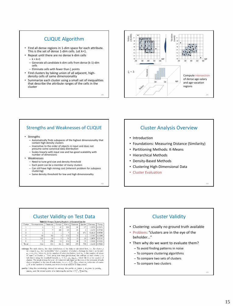
CLIQUE Algorithm

• Find all dense regions in 1-dim space for each attribute. This is the set of dense 1-dim cells. Let k=1.

• Repeat until there are no dense k-dim cells – k = k+1 – Generate all candidate k-dim cells from dense (k-1)-dim

cells – Eliminate cells with fewer than points

• Find clusters by taking union of all adjacent, high-density cells of same dimensionality

• Summarize each cluster using a small set of inequalities that describe the attribute ranges of the cells in the cluster

100 101

Sala

ry

(10

,00

0)

20 30 40 50 60 age

5

4

3

1

2

6

7

0

20 30 40 50 60 age

5

4

3

1

2

6

7

0

Vaca

tion

(wee

k)

age

Vaca

tion

30 50

= 3

Compute intersection of dense age-salary and age-vacation regions

Strengths and Weaknesses of CLIQUE

• Strengths – Automatically finds subspaces of the highest dimensionality that

contain high-density clusters – Insensitive to the order of objects in input and does not

presume some canonical data distribution – Scales linearly with input size and has good scalability with

number of dimensions

• Weaknesses – Need to tune grid size and density threshold – Each point can be a member of many clusters – Can still have high mining cost (inherent problem for subspace

clustering) – Same density threshold for low and high dimensionality

102


• Introduction







103

Cluster Validity on Test Data

104

Cluster Validity

• Clustering: usually no ground truth available

• Problem: “clusters are in the eye of the beholder…”

• Then why do we want to evaluate them?

– To avoid finding patterns in noise

– To compare clustering algorithms

– To compare two sets of clusters

– To compare two clusters

105

16

Clusters found in Random Data

106

0 0.2 0.4 0.6 0.8 10

0.1

0.2

0.3

0.4

0.5

0.6

0.7

0.8

0.9

1

x

y

Random

Points

0 0.2 0.4 0.6 0.8 10

0.1

0.2

0.3

0.4

0.5

0.6

0.7

0.8

0.9

1

x

y

K-means

0 0.2 0.4 0.6 0.8 10

0.1

0.2

0.3

0.4

0.5

0.6

0.7

0.8

0.9

1

xy

DBSCAN

0 0.2 0.4 0.6 0.8 10

0.1

0.2

0.3

0.4

0.5

0.6

0.7

0.8

0.9

1

x

y

Complete

Link

Measuring Cluster Validity Via Correlation

• Two matrices – Similarity Matrix – “Incidence” Matrix

• One row and one column for each object • Entry is 1 if the associated pair of objects belongs to the same cluster,

otherwise 0

• Compute correlation between the two matrices – Since the matrices are symmetric, only the correlation between

n(n-1) / 2 entries needs to be calculated.

• High correlation: objects close to each other tend to be in same cluster

• Not a good measure when clusters can be non-globular and intertwined

107

Measuring Cluster Validity Via Correlation

109

0 0.2 0.4 0.6 0.8 10

0.1

0.2

0.3

0.4

0.5

0.6

0.7

0.8

0.9

1

x

y

0 0.2 0.4 0.6 0.8 10

0.1

0.2

0.3

0.4

0.5

0.6

0.7

0.8

0.9

1

x

y

Corr = 0.9235 Corr = 0.5810

Similarity Matrix for Cluster Validation

• Order the similarity matrix with respect to cluster labels and inspect visually – Block-diagonal matrix for well-separated clusters

110

0 0.2 0.4 0.6 0.8 10

0.1

0.2

0.3

0.4

0.5

0.6

0.7

0.8

0.9

1

x

y

Points

Po

ints

20 40 60 80 100

10

20

30

40

50

60

70

80

90

100Similarity

0

0.1

0.2

0.3

0.4

0.5

0.6

0.7

0.8

0.9

1


• Clusters in random data are not so crisp

111

Points

Po

ints

20 40 60 80 100

10

20

30

40

50

60

70

80

90

100Similarity

0

0.1

0.2

0.3

0.4

0.5

0.6

0.7

0.8

0.9

1

DBSCAN

0 0.2 0.4 0.6 0.8 10

0.1

0.2

0.3

0.4

0.5

0.6

0.7

0.8

0.9

1

x

y



112

Points

Po

ints

20 40 60 80 100

10

20

30

40

50

60

70

80

90

100Similarity

0

0.1

0.2

0.3

0.4

0.5

0.6

0.7

0.8

0.9

1

K-means

0 0.2 0.4 0.6 0.8 10

0.1

0.2

0.3

0.4

0.5

0.6

0.7

0.8

0.9

1

x

y

17



113

0 0.2 0.4 0.6 0.8 10

0.1

0.2

0.3

0.4

0.5

0.6

0.7

0.8

0.9

1

x

y

Points

Po

ints

20 40 60 80 100

10

20

30

40

50

60

70

80

90

100Similarity

0

0.1

0.2

0.3

0.4

0.5

0.6

0.7

0.8

0.9

1

Complete Link


114

1 2

3

5

6

4

7

DBSCAN

0

0.1

0.2

0.3

0.4

0.5

0.6

0.7

0.8

0.9

1

500 1000 1500 2000 2500 3000

500

1000

1500

2000

2500

3000

Sum of Squared Error

• For fixed number of clusters, lower SSE indicates better clustering – Not necessarily true for non-globular, intertwined clusters

• Can also be used to estimate the number of clusters – Run K-means for different K, compare SSE

115

2 5 10 15 20 25 300

1

2

3

4

5

6

7

8

9

10

K

SS

E

5 10 15

-6

-4

-2

0

2

4

6

When SSE Is Not So Great

116

1 2

3

5

6

4

7

SSE of clusters found using K-means

Comparison to Random Data or Clustering

• Need a framework to interpret any measure – E.g., if measure = 10, is that good or bad?

• Statistical framework for cluster validity – Compare cluster quality measure on random data or

random clustering to those on real data • If value for random setting is unlikely, then cluster results are

valid (cluster = non-random structure)

• For comparing the results of two different sets of cluster analyses, a framework is less necessary – But: need to know whether the difference between

two index values is significant

117

Statistical Framework for SSE

• Example: found 3 clusters, got SSE = 0.005 for given data set • Compare to SSE of 3 clusters in random data

– Histogram: SSE of 3 clusters in 500 sets of random data points (100 points from range 0.2…0.8 for x and y)

– Estimate mean, stdev for SSE on random data – Check how many stdev away from mean the real-data SSE is

118

0.016 0.018 0.02 0.022 0.024 0.026 0.028 0.03 0.032 0.0340

5

10

15

20

25

30

35

40

45

50

SSE

Co

unt

0 0.2 0.4 0.6 0.8 10

0.1

0.2

0.3

0.4

0.5

0.6

0.7

0.8

0.9

1

x

y

Random data

18

Statistical Framework for Correlation

• Compare correlation of incidence and proximity matrices for well-separated data versus random data

119

0 0.2 0.4 0.6 0.8 10

0.1

0.2

0.3

0.4

0.5

0.6

0.7

0.8

0.9

1

x

y

0 0.2 0.4 0.6 0.8 10

0.1

0.2

0.3

0.4

0.5

0.6

0.7

0.8

0.9

1

x

y

Corr = - 0.9235 Corr = - 0.5810

Random data

Cluster Cohesion and Separation

• Cohesion: how closely related are objects in a cluster – Can be measured by SSE (mi = centroid of cluster i):

• Separation: how well-separated are clusters – Can be measured by between-cluster sum of squares (m =

overall mean):

120

ii Ci ii C

iC yxx

yxmx,

22 )(2

1)(SSE

i

iiC 2)(BSS mm

cohesion separation

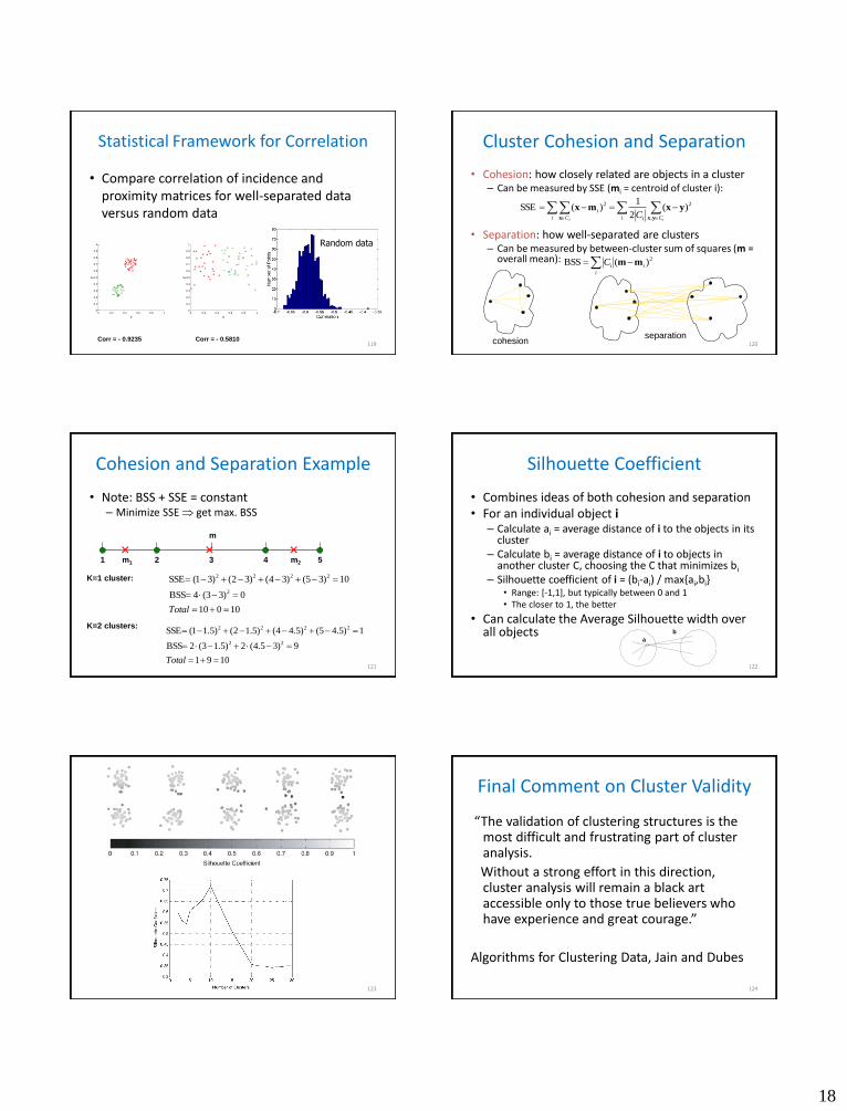
Cohesion and Separation Example

• Note: BSS + SSE = constant – Minimize SSE get max. BSS

121 1091

9)35.4(2)5.13(2BSS

1)5.45()5.44()5.12()5.11(SSE

22

2222

Total

1 2 3 4 5 m1 m2

m

K=2 clusters:

10010

0)33(4BSS

10)35()34()32()31(SSE

2

2222

Total

K=1 cluster:

Silhouette Coefficient

• Combines ideas of both cohesion and separation • For an individual object i

– Calculate ai = average distance of i to the objects in its cluster

– Calculate bi = average distance of i to objects in another cluster C, choosing the C that minimizes bi

– Silhouette coefficient of i = (bi-ai) / max{ai,bi} • Range: [-1,1], but typically between 0 and 1 • The closer to 1, the better

• Can calculate the Average Silhouette width over all objects

122

a

b

123

Final Comment on Cluster Validity

“The validation of clustering structures is the most difficult and frustrating part of cluster analysis.

Without a strong effort in this direction, cluster analysis will remain a black art accessible only to those true believers who have experience and great courage.”

Algorithms for Clustering Data, Jain and Dubes

124

19

Summary

• Cluster analysis groups objects based on their similarity (or distance) and has wide applications

• Measure of similarity (or distance) can be computed for all types of data

• Many different types of clustering algorithms – Discover different types of clusters

• Many measures of clustering quality, but absence of ground truth always a challenge

125

cluster analysis overview data mining techniques ...€“as a preprocessing step for other...

Documents