cluster ensemble statistics of body particle system

Cluster Ensemble Statistics of Body Particle System

Zhong-Cheng Liang

School of Electronic and Optical Engineering, Nanjing University of Posts and Telecommunications, Nanjing, China E-mail: [email protected]

Abstract. A theory of cluster ensemble statistics is developed based on the body particle model. Cluster ensemble is a set of temporal snapshots of particle configuration, which is accurately described by a cluster matrix. The partition functions of liquid, solid and gas are calculated in the statistical zones of the energy space, which directly reveals the relationship between the volume and motional energies. The motional energies of liquid, solid and gas are expressed by the statistical correlations of the particle mass, the rotary inertia and the elastic modulus, respectively. Complete energy relations and equations are derived through the statistics of cluster ensemble. Thermodynamic laws and equations can be logically inferred from the theoretical results. Two types of phase transition mechanism are analyzed based on the theory of body particles and the structure of the energy space.

Keywords: Particle and cluster, ensemble statistics, partition function, order parameter, thermodynamic laws, phase transition

1 Introduction

What is a particle? This is the fundamental problem of physics. Current physics is a magnificent building based on the ideal models of point-like and wave-like particles. Point-like and wave-like particles are cornerstones of classical physics and modern physics, respectively. However, they are so idealized models that lose the physical authenticity. Point-like and wave-like particles do not contain interactions themselves. Interaction is the property imposed to the particles by the aid of mechanical laws. For examples, the gravitational and electromagnetic interactions are described by the Newton law and Lorenz force [1,2]. The weak and strong interactions are presented through Hamiltonian operator or Lagrangian integral [3,4]. As for the origins of mass, charge, color, taste, etc., they cannot be explained by the ideal model itself. Therefore, the unification of fundamental interactions remains an unsolved problem in physics.

Mathematical abstraction is necessary, but it cannot be divorced from physical reality. Real particles are three-dimensional object with both mass and volume, which are called body particles. The fundamental characteristic of body particles is that the volumes of different particles do not intersect in space, which is called volume repulsion. Volume repulsion is exactly what is missing for point-like and wave-like particles. Point or wave abstraction allows different particles to overlap in space, which leads to the singularity of particle density and the difficulty in wave function interpretation. String theory tries to unify the fundamental interactions by replacing the point-like and wave-like particles with string-like particles in ten-dimensional space [5]. The unusual feature of string theory leads to extremely complicated mathematics, which is far beyond the understanding ability of ordinary people and the scope of experimental verification.

There are good reasons to believe that the theories based on the point-like and wave-like particle are the approximation of real particles. A common feeling is that the mathematical concepts for dealing with waves and strings are highly abstract, and the mathematical tools for dealing with real particles are bound to be extremely complicated. This is a great misunderstanding. Three years ago, the author put forward the body particle model and established a new physical theory [6]. Its simplicity, consistency and universality are far beyond expectation. Body particles are objects with only mass and volume, and all objects can be regarded as a system comprised of separate body particles. The state of an object is completely described by the set theory. The main mathematical tools for dealing with body particle systems are statistics and calculus, from which the general laws of physics are derived. The author has established a particle field theory based on mass and momentum statistics [6,7,8], and an energy state theory based on energy statistics [6,9]. The author also proposed an ensemble statistical method [6] to

New Horizons in Mathematical Physics, Vol. 3, No. 2, June 2019 https://dx.doi.org/10.22606/nhmp.2019.32002 53

Copyright © 2019 Isaac Scientific Publishing NHMP

calculate the statistical function of liquids. This article perfects the theory of ensemble statistics and applies it to whole energy spaces. We calculate the statistical functions of liquid, solid and gas, derive the thermodynamic relations and fundamental equations, and finds the general laws of state change and phase transition in the energy space.

2 Concepts and Principles

As a systematic theory different from classical physics and modern physics, it is necessary to rehearsal the original concepts and basic principles [6-9].

2.1 Principle of Object Structure

(1) Object. An object is three-dimensional entity that has only mass and volume. (2) Particle. A particle is three-dimensional entity that has only mass and volume. Such particle is

termed body particle in contrast to the point particle. (3) Axiom of object structure (Axiom 1). Any object is composed of particles with nesting structure. An

object can be decomposed into discrete and finite particles. (4) Primary particle: A primary particle is indivisible particle that has constant mass. (5) Axiom of primary particle (Axiom 2). There are only two types of primary particles of different mass:

proton and electron. (6) Theorem of mass imperishability. Mass is an inherent property of particles, and the mass of a primary

particle is constant. All objects are made up of primary particles, so the mass of an object cannot be annihilated.

2.2 Principles of Space, Time and Motion

(1) Space. Space is the place in which the objects exist and move. The real space is continuous, uniform and three-dimensional.

(2) Axiom of real space (Axiom 3). Real space is filled with particles. There exists no empty space that has no particles.

(3) Time. Time is a progression with which the objects exist and move. The time is continuous, uniform and unidirectional.

(4) Motion. Motion is the process that the state of object changes with time in space. (5) Volume. The volume of an object is the space required for the motion of its internal particles. (6) Theorem of volume repulsion. The motion of particles requires space and time. The volume of

different particles does not intersect each other in real space at the same time. (7) Real physics. Real physics is a theory based on real space and restricted in the domain (field) of real

number.

2.3 Principle of Objectivity

(1) Physical quantity. Any physical quantity can be decomposed as the product of scale and digit .

∙ ; 0. (1) The scale is the unit of measurement and the identification of the physical quantity, while the digit is the number of the physical quantity. The scale is a scalar in the domain of positive real number. Depending on the type of physical quantity, the digit can be a scalar, a vector or a tensor.

(2) Objective and subjective quantity. The physical quantity is objective quantity, and the scale is subjective quantity.

(3) Absolute and relative quantity. The physical quantity is absolute quantity, and the digit is relative quantity.

(4) Axiom of objectivity (Axiom 4). The physical quantities are objective and the laws of motion are objective. Physical theory must exclude all subjective factors. The objectivity axiom requires the object measurability, the origin irrelevance, and the scale irrelevance.

54 New Horizons in Mathematical Physics, Vol. 3, No. 2, June 2019

NHMP Copyright © 2019 Isaac Scientific Publishing

(5) Object measurability. Objects are measurable, immeasurable things are subjective. A measurable quantity is finite and has scale, which requires 0.

(6) Origin irrelevance. The reference points of space and time are subjective and relative. All physical formulas must be independent of the origins of space and time.

(7) Scale irrelevance. Any physical relation , is independent of the scales, i.e. the physical relation and digital relation are equivalent, , ∙ ̃; ̃ , . (2)

The axiom of objectivity is essentially the principle of universality. The origin irrelevance means that the physical laws are applicable to any place and any time. The scale irrelevance means that the physical laws are applicable to any scale. For example, there should be no difference between microphysics and macrophysics.

3 Motion and Energy

3.1 Structure of Object

An object is a particle system, which can be expressed by the particle set | 1,2,3,⋯ , . The structure of an object contains particles of different layers, such as primary particles (protons and electrons), atoms and molecules. The nesting model of object structure is: top-particle ⊇ meso-particle ⊇ base-particle ⊇ sub-particle. That is, an upper layer comprises all lower layers, e.g., the object contains molecules and the molecules contain atoms. The top-particle is the object under study, and the base-particles are the basic blocks of the object. The number of base-particles is the statistical cardinality of the object [9].

3.2 Modes of Motion

With the mass center as origin and the principal axes , , as directions, we construct a reference frame for any body particle. The frame is called the principal axes frame represented by

. With the aid of principal axes frame, the spatial state of a body particle is described as position, posture and profile. Correspondingly, the motion of the particle can be decomposed into three modes of translation, rotation and vibration. Translation is the position change of the center of mass, rotation is the direction change of the principal axes, and vibration is the profile oscillation accompanied by the change of the principal rotary inertias [9].

Each motion mode has 3 degrees of freedom, each particle has 9 degrees of freedom, and an object composed of base-particles has 9 degrees of freedom. The total vibratory energy , total rotary energy , and total translatory energy of the object are obtained by separately summing the energy of the three modes of motion.

∙ ; , .

∙ ; , . (3)

∙ ; , .

In Eq.(3), is the scale of vibratory energy (vibtration quantum), is the scale of rotary energy (rotation quantum), and is the scale of translatory energy (translation quantum). , , are the vibration constant (Planck constant), the rotation constant and the translation constant (Boltzmann constant), respectively. , , are the vibration intensity (frequency), the rotation intensity and the translation intensity (thermodynamic temperature), respectively.

3.3 Space of Energy

Energy space is a set of ordered array constructed by , , and . The basic definitions and relations of energy space parameters [9] are listed in Table 1.

New Horizons in Mathematical Physics, Vol. 3, No. 2, June 2019 55


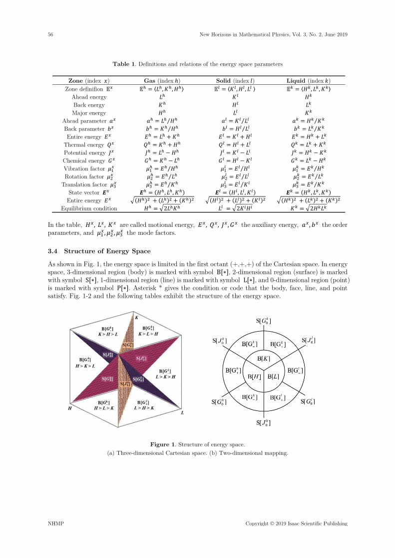
Table 1. Definitions and relations of the energy space parameters

Zone (index ) Gas (index ) Solid (index ) Liquid (index )Zone definifion ⟨ , , ⟩ ⟨ , , ⟩ ⟨ , , ⟩

Ahead energy Back energy Major energy

Ahead parameter ⁄ ⁄ ⁄ Back parameter ⁄ ⁄ ⁄ Entire energy

Thermal energy Potential energy Chemical energy Vibration factor ⁄ ⁄ ⁄ Rotation factor ⁄ ⁄ ⁄

Translation factor ⁄ ⁄ ⁄ State vector , , , , , ,Entire energy

Equilibrium condition 2 2 2 In the table, , , are called motional energy, , , , the auxiliary energy, , the order parameters, and , , the mode factors.

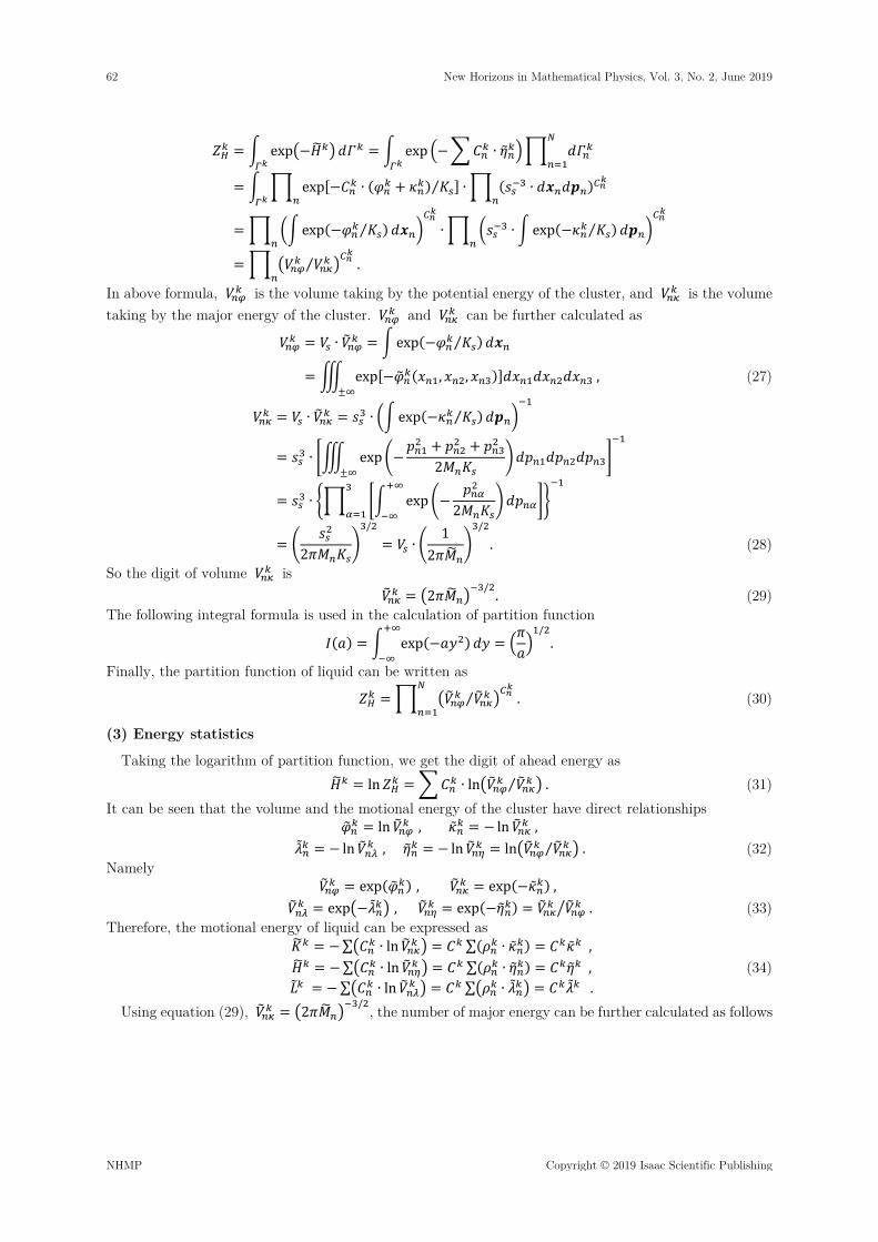
3.4 Structure of Energy Space

As shown in Fig. 1, the energy space is limited in the first octant (+,+,+) of the Cartesian space. In energy space, 3-dimensional region (body) is marked with symbol B ∗ , 2-dimensional region (surface) is marked with symbol S ∗ , 1-dimensional region (line) is marked with symbol L ∗ , and 0-dimensional region (point) is marked with symbol P ∗ . Asterisk * gives the condition or code that the body, face, line, and point satisfy. Fig. 1-2 and the following tables exhibit the structure of the energy space.

Figure 1. Structure of energy space. (a) Three-dimensional Cartesian space. (b) Two-dimensional mapping.



Figure 2. (a) Phase interfaces, translation equilibrium surface and isoenergy surface. (b) Equilibrium surfaces of vibration, rotation and translation.

Table 2. Zones and phases

Gas zone B Solid zone B Liquid zone B B B B B B B

Table 3. Phase interfaces

Name Symbol Condition

J-type interface (planes of zero potential energy)

S 0 S 0 S 0

G-type interface (planes of zero chemical energy)

S 0 S 0 S 0

Table 4. Order parameters

Zone Ahead parameter Back parameter Equilibrium condition Range B ⁄ ⁄ 2 1 1 2⁄ , 1B ⁄ ⁄ 2 1 1 2⁄ , 1B ⁄ ⁄ 2 1 1 2⁄ , 1

Table 5. Equilibrium surfaces

Name Symbol Condition Vibration surface S √2 Rotation surface S √2

Translation surface S √2

Table 6. Structure of equilibrium surfaces

Zone\Phase B B B B B B S S S S S S S S S S S S



4 Cluster Ensemble Statistics

Cluster ensemble is a set of snapshots of particle configurations, and its principle is similar to that of the computer tomography. Cluster ensemble statistics is a new method based on the concepts of body particles and energy space. This section explains the statistical principle and calculates the statistical functions of gas, liquid and solid.

4.1 Statistical Principle

(1) Object and cells

Imagine an object as a container with boundary and volume , in which base-particles are contained. These particles are constantly moving, including translation, rotation and vibration. Because of the volume repulsion, the different particles do not intersect in space, so the density of particles in the container is limited.

In order to study the distribution of particles, it is necessary to divide the volume of an object with unit cells of identical shape. The unit cell is a cube with volume which is called volume quantum. Then, the object has the total number of cells ⁄ . (4) If there are particles in the -th cell, the particle density of the cell is ⁄ . The total number of particles is ∑ and the average number of particles per cell is ⁄ .

(2) Ensemble and cluster

Now we take the snapshots of the particle configuration in a time sequence, ∙ , 1,2,⋯ , ,⋯ , with the time quantum ⁄ . The set of these snapshots is called a statistical

ensemble. In the ensemble, the number of snapshots is , and the total number of cells is . The set of particles in one cell is called a cluster. The cluster of particles is called a -cluster denoted

by . The total number of -clusters in the ensemble is denoted by . To number the particles by 1,2,⋯ , implies that the particles are distinguishable. To avoid confusion, the example particles in

this article are numbered in capital letters (see Fig. 3). Because of the persistent motion of particles [9], each particle has the possibility to enter all cells. Which

particles enter the same cell to form a cluster is random, but constrained by volume repulsion. Volume repulsion restricts the number of particles that can be accommodated in one cell. The number of -clusters

is a statistical description of the state of the object. Macroscopic properties of an object can be given either by particle statistics or by cluster statistics. According to the object structure model, cluster is the meso-particle between base-particle and top-particle [9]. An example of cluster is the gridon in particle field theory [7,8].

(3) Cluster matrix

The clusters of an ensemble are characterized by a matrix with the element . The matrix element represents the number of -clusters in the -th snapshot. For example, Fig. 3 shows four snapshots of the ensemble (drawn as two-dimensional graph for clarity). This ensemble has cells 9 and particles 10. The particles are marked by A, B, C, D, E, F, G, H, I and J. The first four snapshots are marked by 1,2,3,4.

1. B, D, H, I, J are 1-clusters, CF is 2-cluster, AEG is 3-cluster. The matrix elements are 5, 1, 1, and the rest is zero. In this snapshot, the number of clusters is 7 and

the number of particles is 1 ∙ 2 ∙ 3 ∙ 10. 2. A, C, D, J are 1-clusters, BF, GI and EH are 2-clusters. The matrix elements are 4, 3, and the rest is zero. In this snapshot, the number of clusters is 7 and the number of

particles is 1 ∙ 2 ∙ 10. 3. C, D, E, G, H, J are 1-clusters, AI and BF are 2-clusters. The matrix elements are 6, 2, and the rest is zero. In this snapshot, the number of clusters is 8 and the number of

particles is 1 ∙ 2 ∙ 10.



4. C, F, G, H, J are 1-clusters, BE is 2-cluster, ADI is 3-cluster. The matrix elements are 5, 1, 1, and the rest is zero. In this snapshot, the number of clusters is 7 and the number of particles is 1 ∙ 2 ∙ 3 ∙ 10.

Figure 3. Sketch map for statistical principle of cluster ensemble. Four snapshots at time 1,2,3,4.

Table 7 lists the elements of cluster matrix of the first ten snapshots ( 1,2,3,⋯ ,10.). For clarity, we use spaces to denote the elements that equal to zero.

Table 7. Example of cluster matrix for 10 10

1 2 3 4 5 6 7 8 9 10

1 5 4 6 5 3 4 3 6 5 4 4.5 2 1 3 2 1 2 1 2 2 1 3 1.8 3 1 1 1 1 1 0.5 4 1 0.1 ⁞ 9 10 ∗ 7 7 8 7 6 6 6 8 7 7 6.9

(4) Matrix property

Firstly, let’s look at the column elements. The sum of the elements of each column is ∗ ∑ . They are ∗ 7, ∗ 7, ∗ 8, ∗ 7, ∗ 6, ∗ 6, ∗ 6, ∗ 8, ∗ 7, ∗ 7. ∗ are placed in the last row of the table 7. Because the particle number in each snapshot is constant, for

each column it has ∑ ∙ 10. Calculating the time average of ∗ gets the total number of clusters, ∑ ∗ 10⁄ 6.9 10, which is put in the last column and the last row of the table.

Then, let’s look at the row elements. The time average of each row elements is ∑ 10⁄ . They are 4.5, 1.8, 0.5, 0.1, 0. are placed in the last column of the table. The total number of clusters is obtained by summing the last column of the table, ∑ 6.9. The total number of particles can also be obtained according to the formula

∑ ∙ 10.



In general, the element forms a cluster matrix. Because the number of particles in each snapshot is conserved, the elements of the -th column satisfy following relationship

∙ . (5)

As all particles experience the same time, the total time experienced by all particles in the ensemble is

∙ ∙ ∙ . (6)

Above equation can be rewritten as

∙1

. (7)

Let 1

, (8)

is the time average of the elements in the -th row of the matrix, which is the number of -clusters in the ensemble. Thus, Eq. (7) can be written in the form

∙ . (9)

Formula (9) stands for the conservation of total number of particles. The sum of gives the total number of clusters of the ensemble

1. (10)

It is seen that the total number of clusters is the time average of the sum of all matrix elements. The cluster number is not greater than the particle number because the total number of particles is conserved.

In addition, we define the sum of column elements as the number of transient clusters

∗ ≡ . (11)

The total number of clusters can also be calculated by the time average of the transient clusters 1

∗1

. (12)

The ensemble average is actually an average over time. Because the time intervals between adjacent snapshots are equal, changing the time order of snapshots will not affect the statistical results.

(5) Statistical equilibrium

If the structure of clusters is stable and the number of clusters does not change with time, this ensemble reaches a state of statistical equilibrium. The condition of statistical equilibrium is expressed as . (13) For nonequilibrium ensemble, , we define a nonequilibrium factor ≡ ⁄ . (14) For equilibrium ensemble, it has 1 . Table 7 is an example of nonequilibrium ensemble with nonequilibrium factor 6.9 9⁄ 0.77.

(6) Statistical constraint

In the energy space, the digit of major energy is , , . (15) If the digit of back energy equals the number of clusters , , , (16) then, the cluster ensemble and the energy space are isomorphic. Eq. (16) is called the isomorphic constraint on the cluster ensemble. Under this constraint, the back parameter becomes

≡ , ≡ , ≡ . (17) The equilibrium condition (13) can be written as

, , . (18) Eq. (18) is called equilibrium constraint on the cluster ensemble.



(7) Cluster statistics

The probability of -cluster is defined as

≡ , ≡ 1. (19)

Without causing confusion, the symbol ∑ ∗ for cluster summation is thereafter simplified to ∑ ∗ . For -cluster, , , , , , , stand for the vibratory energy, rotary energy, translatory energy,

entire energy, thermal energy, potential energy and chemical energy, respectively. The total motional energy and auxiliary energy can be calculated by cluster ststistics. ∑ ∑ , ∑ . ∑ ∑ , ∑ . ∑ ∑ , ∑ . ∑ ∑ , ∑ . (20) ∑ ∑ , ∑ . ∑ ∑ , ∑ . ∑ ∑ , ∑ . In above formulas, , , , , , , are the average energies per cluster.

4.2 Liquid Statistics

(1) Statistical zone

The zone index of liquid is . The -cluster in liquid zone is denoted by , and the number of is denoted by . Let the principal axes frame at the time be , at the time

1 be . Then, , , is the translation and , , is the translatory momentum of the cluster . The statistical zone of the cluster, , is constitutes by the parameters , , , , , . Let and , we express the volume element of as ∙ , . (21) The liquid statistical zone consisting of all clusters is , with the zone volume element

∙ , 1. (22)

(2) Partition function

The partition function of liquid is defined as

≡ exp , (23)

where exp is the probability density of the ahead energy (vibratory energy). Partition function is the integral of probability density in the liquid statistical zone .

The potential energy of the cluster, , can be expressed by the translation , , as , , . (24) The major energy (translatory energy) of the cluster, , can be expressed by the translatory momentum

, , as

2, (25)

where is the mass of cluster . The energy scale of liquid is . Due to , the digits of ahead energy (vibratory

energy ) for the cluster and the liquid are ⁄ ⁄ ,

∙ ∙ ⁄ . (26) Substituting and into , the partition function of the liquid is calculated as follows



exp exp ∙

exp ∙ ⁄ ∙ ∙

exp ⁄ ∙ ∙ exp ⁄

⁄ .

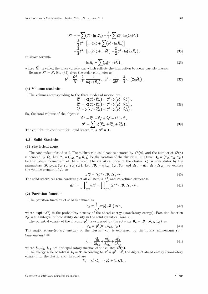
In above formula, is the volume taking by the potential energy of the cluster, and is the volume taking by the major energy of the cluster. and can be further calculated as

∙ exp ⁄

exp , , , (27)

∙ ∙ exp ⁄

∙ exp2

∙ exp2

2

/

∙1

2

/

. (28)

So the digit of volume is 2

/. (29)

The following integral formula is used in the calculation of partition function

exp/.

Finally, the partition function of liquid can be written as

⁄ . (30)

(3) Energy statistics

Taking the logarithm of partition function, we get the digit of ahead energy as ln ∙ ln ⁄ . (31)

It can be seen that the volume and the motional energy of the cluster have direct relationships ln , ̃ ln ,

ln , ln ln ⁄ . (32) Namely

exp , exp ̃ , exp , exp . (33) Therefore, the motional energy of liquid can be expressed as ∑ ∙ ln ∑ ∙ ̃ ̃ , ∑ ∙ ln ∑ ∙ , (34) ∑ ∙ ln ∑ ∙ .

Using equation (29), 2/ , the number of major energy can be further calculated as follows



∙ ln32∙ ∙ ln 2

32

∙ ln 2 ∙ ln

32

∙ ln 2 ln32

∙ ln 2 . (35) In above formula

ln ∙ ln , (36) where is called the mass correlation, which reflects the interaction between particle masses.

Because , Eq. (35) gives the order parameter as 23∙

1

ln 2,

12

34∙ ln 2 . (37)

(4) Volume statistics

The volumes corresponding to the three modes of motion are ∑ ∙ ∙ ∑ ∙ , ∑ ∙ ∙ ∑ ∙ , (38) ∑ ∙ ∙ ∑ ∙ . So, the total volume of the object is

∙ ,

. (39) The equilibrium condition for liquid statistics is 1.

4.3 Solid Statistics


The zone index of solid is . The -cluster in solid zone is denoted by , and the number of is denoted by . Let , , be the rotation of the cluster in unit time, , , be the rotary momentum of the cluster. The statistical zone of the cluster, , is constitutes by the parameters , , , , , . Let and , we express the volume element of as ∙ , (40) The solid statistical zone consisting of all clusters is , and its volume element is

∙ . (41)


The partition function of solid is defined as

≡ exp , (42)

where exp is the probability density of the ahead energy (translatory energy). Partition function is the integral of probability density in the solid statistical zone . The potential energy of the cluster, , is expressed by the rotation , , as

, , . (43) The major energy(rotary energy) of the cluster, , is expressed by the rotary momentum

, , as

2 2 2, (44)

where , , are principal rotary inertias of the cluster . The energy scale of solid is . According to , the digits of ahead energy (translatory

energy ) for the cluster and the solid are ̃ ⁄ ⁄ ,



∙ ̃ ∙ ⁄ . (45) Similar to the case of liquid, we can calculate the partition function of solid by substituting and

into . The result is

⁄ , (46)

where and are the cluster volumes of the potential energy and the major energy, respectively.

exp ⁄

exp , , , (47)

∙ exp ⁄

∙ exp12

exp̃

2̃ 2 /

2 / , . (48)


The digit of ahead energy is obtained by taking the logarithm of the partition function ln ∙ ln ⁄ . (49)

The volume and the motional energy of the cluster have following relationships exp , exp ,

exp , exp ̃ . (50) Therefore, the motional energy of the solid can be expressed as ∑ ∙ ln ∑ ∙ , ∑ ∙ ln ∑ ∙ ̃ ̃ , (51) ∑ ∙ ln ∑ ∙ . Using equation (48), 2 / , we have

∙ ln32

∙ ln 2 , ln ∙ ln . (52) where is called the inertia correlation. Because , Eq. (52) gives the order parameter of solid as

23∙

1

ln 2,

12

34∙ ln 2 . (53)



∙ ,

. (55) The equilibrium condition for solid statistics is 1.

4.4 Gas Statistics




The zone index of gas is . The -cluster in gas zone is denoted by , and the number of is denoted by . Let , , be the deformation of the cluster and , , be the stress of the cluster. The statistical zone of the cluster, , is constitutes by the parameters

, , , , , . Let and , we express the volume element of as ∙ , (56) The gas statistical zone consisting of all clusters is , and its volume element is

∙ . (57)


The partition function of gas is defined as

≡ exp , (58)

where exp is the probability density of ahead energy (rotary energy). Partition function is the integral of the probability density in statistical zone .

The potential energy of the cluster, , is expressed by the deformation , , as , , . (59) The major energy (vibratory energy) of the cluster, , is expressed by the stress , , as

∙2 2 2

, (60)

where , , are principal elastic modulus of the cluster . The energy scale of gas is . According to , the digits of ahead energy (rotary

energy ) for the cluster and the gas are ⁄ ⁄ ,

∙ ∙ ⁄ . (61)

The partition function of gas is calculated by substituting and into . The result is

, (62)

where and are the cluster volumes of the potential energy and the major energy, respectively.

exp ⁄

exp , , , (63)

∙ exp ⁄

∙ exp2

exp2

2/

2/, . (64)


The digit of ahead energy is obtained by taking the logarithm of the partition function ln ∙ ln . (65)

The volume and the motional energy of the cluster have following relationships exp , exp ,

exp ̃ , exp . (66) Therefore, the motional energy of the gas can be expressed as



∑ ∙ ln ∑ ∙ , ∑ ∙ ln ∑ ∙ , (67) ∑ ∙ ln ∑ ∙ ̃ ̃ . Using equation (64), 2

/ , we have

∙ ln32

∙ ln 2 , ln ∙ ln . (68) where is called the modulus correlation. Because , Eq. (68) gives the order parameter of gas as

23∙

1

ln 2,

12

34∙ ln 2 . (69)



∙ ,

. (71) The equilibrium condition for gas statistics is 1.

5 Liquid Thermodynamics

This section derives the thermodynamic functions and equations, and compares them with classical thermodynamic theory [10]. Because the three energy zones have even permutation symmetry, we only study the liquid zone ⟨ , , ⟩ as an example. The situation of gas and solid can be analyzed in the same way. Without causing confusion, we omit the zone index in this section.

5.1 Thermodynamic Functions

(1) Motional energy

For liquid zone, the ahead energy is (vibratory energy), the back energy is (rotary energy), and the major energy is (translatory energy). The energy scale is . The order parameters and the equilibrium condition are ⁄ , ⁄ ,2 1. (72) and are ahead parameter and back parameter, respectively. The motional energy can be decomposed by the number of particles as

, . , . (73) , .

According to the constraint , the motional energy can be decomposed by the number of clusters. , . , . (74) , .

Because , we also have , . , . (75) , .

(2) Auxiliary energy

The auxiliary energy is decomposed by the number of particles as



, . 1 , 1 . 1 , 1 . (76) , . The auxiliary energy is decomposed by the number of clusters as 1 , 1 . 1 1 , 1 . 1 1 , 1 . (77) 1 , 1 . , , , are cluster energies, among them is called thermal potential, and is called chemical

potential.

(3) Internal energy and enthalpy

Now we introduce other two auxiliary functions, the interal energy and the enthalpy . ≡ , ≡ 2 . (78) They can be decomposed by the number of particles as 1 , 1 . 1 2 , 1 2 . (79) They can be decomposed by the number of clusters as 1 , 1 . 1 2 , 1 2 . (80)

(4) Entropy

The ratio of thermal energy to temperature is defined as thermal entropy , and the ratio of chemical energy to temperature is defined as chemical entropy , ≡ ⁄ 1 , ≡ ⁄ . (81) The thermal entropy is always positive and the chemical entropy can be positive or negative. The cluster entropy is

≡⁄ ⁄

, ≡⁄ ⁄

. (82) Thermal entropy is an important concept in classical thermodynamics. According to the famous

Boltzmann formula ∙ ln Ω, the thermodynamic probability Ω can be expressed by back parameter Ω exp ⁄ exp 1 . (83)

5.2 Thermodynamic Responsivity

(1) Equation of state

The equation of state of liquid is given by the volume decomposition and the particle decomposition of the entire energy [9]. , ⁄ . (84) where is the density of entire energy and is the mode factor of major energy. The physical dimensions of pressure and energy density are the same, but their physical meanings are different. We called the entire pressure in this section, or just pressure for convenience. The relative changes in temperature, volume and pressure of an object are called thermodynamic responsivity. The responsivity can be calculated by the equation of state.

(2) Isobaric volume responsivity

The isobaric volume responsivity is defined by the volume response with the temperature change at constant pressure

≡1 1 1

. (85)



is similar to the isobaric volume expansion coefficient. In isobaric process ( 0), if 0 ( 0), then ∙ 0. Therefore, this process is limited to the equilibrium surface but not to the isoenergy surface.

(3) Isochoric pressure responsivity

The isochoric pressure responsivity is defined by the pressure response with the temperature change at constant volume.

≡1 1 1

. (86)

is similar to the isochoric coefficient of pressure. In isochoric process ( 0), if 0 ( 0), then ∙ 0. This process is not limited to the isoenergy surface.

(4) Isothermal volume responsivity

The isothermal volume responsivity is defined by the negative value of the volume response with the pressure change at constant temperature.

≡1 1 1

. (87)

is similar to the isothermal compressibility. In isothermal process ( 0), if 0 ( 0, 0), then ∙ ∙ 0. This process is also not limited to the isoenergy surface.

(5) Isoenergy volume responsivity

The isoenergy volume responsivity is defined by the negative value of the volume response with the pressure change at constant entire energy. If ∙ ∙ 0, we have

≡1 1

. (88)

is similar to the adiabatic compressibility. This process takes place along the intersection of the equilibrium surface and the isoenergy surface.

(6) Isobaric energy capacity

The isobaric energy capacity is defined by the change of entire energy with the change of temperature at constant pressure. It can be obtained by using the equation of state and the definition of the isobaric volume responsivity as

≡ ∙ . (89)

(7) Isochoric energy capacity

The isochoric energy capacity is defined by the change of entire energy with the change of temperature at constant volume. It can be obtained by using the equation of state and the definition of isochoric pressure responsivity as

≡ ∙ . (90)

5.3 Thermodynamic Theorems

(1) Generating equation

According to Eqs. (75) and (82), the rotary and thermal energies of cluster are and , respectively. Because , the differential of the translatory energy of the cluster is

. (91) where , . (92) So, we can calculate the differential of chemical energy as



. Because and , we have . (93) Substituting into the above formula, we obtain a relation similar to the Gibbs formula in thermodynamics 0. (94) Above formula is called generating equation.

(2) Energy equations

By Legendre transformation of the generating equation, we can obtain a set of equivalent equations. For example, by substituting into (94), we have , which is called energy equation. For easy of comparison, we list the energy relations and the energy equations of liquid in Table 8.

Table 8. Energy relations and energy equations of liquid

Energy Relation Equation Vibratory energy Rotary energy ,

Translatory energy Thermal energy , Chemical energy ,Internal energy

Enthalpy 2 Zero 0 0

The energy equations of liquids have similar forms to the fundamental thermodynamic relations [10]. A

notable difference is that in the equations represents the density of rotary energy, which is different from the classical concept of pressure. Comparing the liquid energy equations with the fundamental thermodynamic relations, we can see that the thermal energy is the heat quantity, is entropy, is Gibbs free energy, is internal energy, is enthalpy, is Helmholtz free energy, is grand potential of thermodynamics. It will be seen that the thermodynamic laws can be fully derived from the axiom of body particles with the statistics of cluster ensemble.

(3) Thermodynamic laws

Motion persistence theorem [9] contains the third law of thermodynamics. The motion of particles includes three modes of translation, rotation and vibration. The total energies of the three modes are , , , respectively. The non-stop motion of particles ensures the positive definiteness of the motional

energy. 0 , i.e., the thermodynamic temperature cannot reach to zero, which is an expression of the third law of thermodynamics. Positive definiteness of motional energy also includes the non-zero rotation intensity (z 0) and the non-zero vibration intensity ( 0).

The existence of equilibrium state in energy space is the basis of the zeroth law of thermodynamics. There are three equilibrium surfaces in the energy space, in which the translation surface represents the thermal equilibrium, and the equilibrium parameter is the translation intensity (thermodynamic temperature). The other two surfaces represent rotation equilibrium and vibration equilibrium. The equilibrium parameters are rotation intensity and vibration intensity (frequency), respectively.

The equations listed in Table 8 contain the first and second laws of thermodynamics. The present of rotary energy in equations is one of the most important discoveries in the body particle theory. Due to the introduction of rotary energy, a set of consistent and complete thermodynamic relations was discovered. In liquid zone, the vibratory energy is mechanical energy, which can be completely converted into thermodynamic work. The translatory energy includes both the directional motion of the object (which can be converted into work) and the disordered motion of particles (which represents the effect of entropy). Rotary energy can be partially converted into work through volume change, and the unconverted part also contributes to entropy. In the new theory, the thermal energy replaces the heat



amount, and entropy ⁄ comes from both translatory energy and rotary energy. From the expressions of internal energy and thermal energy , we can see that the role of rotary energy is implied in the first law (by internal energy) and the second law (by entropy) of the thermodynamics. The role of rotary energy has not been well recognized in current physics, so it is impossible to reveal the essence of the laws of thermodynamics. The fundamental reason is that the particle model of current physics is too idealized. The point-like particles in classical physics and the wave-like particles in modern physics well describe the motion modes of translation and vibration, respectively, but not well for rotation mode. Only the body particle model can characterize the motion of particle system in a unified way.

6 Phase Transition

6.1 Concept of Phase Transition

As mentioned in section 3.3, the energy space is the first ctant of Cartesian coordinate system with , , as its axes. The energy space is divided into six phases (B , B , , , ) by six interfaces (S , S ). S is called J-type interface which is the plane of zero potential energy. S separate the energy space into three zones. S is called G-type interface which is the plane of zero chemical energy. S divide each zone into two phases, 0 and 0.

Phase transition is a physical process or macroscopic phenomenon in which the state of an object changes from one phase to another. There are two types of phase transition corresponging to the two types of phase interfaces. The transition passing through the plane S is called J-type phase transition, and the transition passing through the plane S is called G-type phase transition.

There are three equilibrium surfaces S , S and S , satisfying √2 , √2 and √2 respectively. The phase transition that keeps two states on the stable equilibrium surface is

equilibrium phase transition, otherwise it is non-equilibrium phase transition. Only equilibrium phase transition is discussed in this article. It is possible for the state of an object to enter the excitation area from the stable area of an equilibrium surface without phase change. That process is called excitation.

6.2 J-type Phase Transition

(1) Two phase equilibrium

The J-type phase transition occurs on the J-type interfaces S . The interfaces S , S and S separate the energy space into three zones B , B and B , representing gas, solid and liquid, respectively.

The straight line where the two equilibrium surfaces intersect is called the transition line. There are three transition lines: gas-solid transition line L S ⋂S , solid-liquid transition line LS ⋂S and liquid-gas transition line L S ⋂S . Since a transition line is located on the interface of two zones, there are two sets of energy in a transition line corresponding to the two zones. Table 9 lists the energies in the transition lines.

Table 9. Energies in transition lines

Surface S S S Line L L L L L L

2 2 2 2 2 2 2 2 2 2 2 2 3 3 3 3 3 3 4 3 4 3 4 3 0 0 0

(2) Phase transition mechanism



The point at the transition line is called the transition point. The process of J-type transition is: when the state in zone reaches at transition point A, it changes along the transition line, and then enters zone at another point B.

For example, the liquid-gas transition line L is a straight line satisfying the relation 2 . The state vectors before and after the transition are

13

2 2 ,13

2 2 . (95) The ahead parameters in the transition line and their difference are 1⁄ , 1 2⁄⁄ ;∆ 1 2.⁄ (96) The difference of potential energy before and after transition is ∆ . (97) The phase transition from liquid to gas absorbs energy, which is called latent energy. The latent energy of liquid-gas transition is equal to the rotary energy of the gas phase.

Similarly, the gas-solid transition line L is a straight line satisfying 2 . The order parameter before and after the phase transition have a 1/2 jump, and the latent energy is equal to the translatory energy of the solid phase . The solid-liquid transition line L is a straight line satisfying 2 . The order parameter before and after the phase transition have a 1/2 jump, and the latent energy equals the vibratory energy of the liquid phase . Generally speaking, J-type phase transition is characterized by the latent energy and 1/2 jump of order parameter.

(3) Liquid-gas phase transition

Take the gas-liquid phase transition as an example. If the phase transition temperature , molar latent energy ∆ , and molar volume and are known, we can determine all the phase transition parameters. (Boltzmann constant 1.38065 10 J ∙ K , Avogadro constant 6.0221410 mole )

Table 10. Parameters of liquid-gas phase transition

Paremeters Liquid state Gas state Molar volume

Vibratory energy 2 Rotary energy 2⁄ ∆

Translatory energy 2 Potential energy 0 Entire energy 3 2⁄ 3 Energy density ⁄ 3 2⁄ ⁄ ⁄ 3 ⁄ Energy scale ⁄ 2 ⁄

Order parameter ⁄ 1 ⁄ 1 2⁄ For example, the phase transition temperature of water at standard atmospheric pressure is

373.15K, the molar latent energy (heat of vaporization) is 40626J, the molar volume of liquid water is 18.612 10 m , The molar volume of water vapor is 30114 10 m . It can be find that 5.1519 10 J , 3102.5J , 1551.3J , 4653.8J , 2.500410 J ∙ m . 81252J, 121878J, 4.0472 10 J ∙ m , 1.3492 10 J.

6.3 G-type Phase Transition

(1) Symmetrical states

The state vectors on the plane S have the following form 12

√2 ,12

√2 ,12

√2 . (98) Because 1,1, √2 are incommensurable, there is no digital state on the plane S . Hence, G-type interface is called the forbidden plane. Unlike J-type transition that occurs on the plane of zero potential energy, G-type phase transition does not occur on the plane of zero chemical energy.



It can be seen from Fig. 2 thatS is the symmetrical plane of two stable areas: S and S . Each stable state on S has a symmetrical state onS . Two stable states with S as the symmetrical plane are called symmetrical states. Symmetrical states have following features: equal major energy, equal entire energy, equal digit and opposite sign chemical energy.

(2) Phase transition mechanism

The G-type transition occurs when the two symmetrical states (S and S ) switch to each other along a phase transition arc (L ). The phase transition arc is a circular arc connecting two stable symmetrical states. It is the intersection of the isoenergetic surface and the stable equilibrium surface.

There are three transition arcs, which are L S ⋂S , L S ⋂S and LS ⋂S . The corresponding equations of the transition arcs are 2 ,

2 and 2 . The G-type phase transition occurs in the same zone, so there are three kinds: gas phase transition, solid

phase transition and liquid phase transition. Examples of G-type transition include ferromagnetic transitions, superconducting and superfluid transitions in condensed matter.

(3) Solid phase transition

For solid, all digital states and energy levels on the rotation equilibrium surface can be easily calculated according to the entire energy and the equilibrium condition 2 . The calculation shows that the symmetrical states on the stable equilibrium surface is sparse. Table 11 lists the four pairs of symmetrical states with the smallest entire energy.

Table 11. Solid symmetrical states

9 8 18 16 25 18 27 24 12 12 24 24 30 30 36 36 8 9 16 18 18 25 24 27 17 17 34 34 43 43 51 51

S S S S S S S S For example, when 17, the vectors of state S and state S are 9i 12j 8k and

8i 12j 9k, respectively. The rotary energy and the entire energy of the two states are unchanged, and the translatory energy and the vibratory energy are converted to each other. The change of order parameter is ∆ 1 12⁄ 0.5 . The changes of thermal energy, chemical energy and potential energy are ∆ 1 , ∆ 2 and ∆ 1 , respectively. Since the entire energy keeps unchanged during the switch of modes of motion, the G-type transition does not exchange energy with the environment. However, the mode switch will inevitably lead to the change of the internal structure of the object.

7 Conclusions

The energy space composed of three motion modes of body particles completely represents the motion state of the object. The energy of objects can be decomposed by volume and number of particles, while the cluster ensemble statistics provides a new way of energy decomposition. Different energy decomposition offers multiple choices for studying the state and structure of the object.

The statistical principle of cluster ensemble is similar to that of computer tomography. Cluster ensemble is a set of isochronous sections of particle configuration in three-dimensional space, and each section is a set of cubic cells with equal volume. Cluster matrix is an accurate description of the cluster ensemble. In principle, knowing the structure and distribution of clusters, one can calculate the mass correlation, inertia correlation and modulus correlation. Knowing the particle number, the energy scale and the statistical correlation, the equilibrium state of an object can be fully determined.

The partition function of cluster ensemble reveals the relationship between the motion, energy and volume of an object. The results show that the motion of particles is the origin of energy and the reason why objects have volume. There are clear quantitative relationships between the volume of an object and



the energy of three modes of motion of the internal particles. In other words, motion generates energy, and energy produces volume.

Cluster statistics gives complete energy relations and differential equations, which include the basic laws of thermodynamics. Particle field theory, energy state theory and cluster ensemble theory used different statistical methods, but they all base on the model of body particles. To understand and explain the physical world from the motion of body particles, its simplicity and consistency make us firmly believe that nature really works according to a unified law. Acknowledgements. This research is partially supported by NSFC (No.61775102). The author sincerely thanks Professor Francis T. S. Yu for his strong support and inspiring discussion. The author also thanks Mr. Ning Tian for his constant encouragement and enthusiastic assistance in many ways.

References

1. S.N. Jin and Y.L. Ma, Theoretical Mechanics, Higher Education Press, Beijing. 2002. 2. S.H. Guo, Electrodynamics, Higher Education Press, Beijing. 2008. 3. J.Y. Zeng, Quantum Mechanics, Science Press, Beijing. 2018. 4. S. Braibant, G. Giacomelli, and M. Spurio. Particles and Fundamental Interactions: An Introduction to Particle

Physics. Springer Netherlands. 2012. 5. B. Zwiebach. A First Course in String Theory. Cambridge University Press, Cambrige. 2004. 6. Z.C. Liang, Physical principles of finite particle system, Scientific Research Publishing, Wuhan. 2015. 7. Z.C. Liang, "Essence of light: particle, field and interaction". in Proc. SPIE (Optics+Photonics, San Diego). 2018.

10755, 1075501-10755014. doi:10.1117/12.2316422. 8. Z.C. Liang, “The origin of gravitation and electromagnetism”. Theoretical Physics, vol. 4, no. 2, pp. 85–102, 2019. 9. Z.C. Liang, “Motion, energy and state of body particle system”. Theoretical Physics, vol. 4, no. 2, pp. 66–84, 2019. 10. Z.H. Lin, Thermodynamics and Statistical Physics, Peking University Press, Beijing, 2007.



cluster ensemble statistics of body particle system

Documents