Linköping University | Department of Computer Science Master Thesis, 30 ECTS | Computer Science

Spring term 2017 | LIU-IDA/LITH-EX-A--17/017—SE

Clustered Data Management in Vir-tual Docker Networks Spanning Geo-Redundant Data Centers

A Performance Evaluation Study of Docker Networking

Hayder Alansari

Supervisor at Tieto: Henrik Leion Supervisor at Linköping University: Ola Leifler Examiner: Cyrille Berger

Linköpings universitet SE–581 83 Linköping +46 13 28 10 00 , www.liu.se

Copyright

The publishers will keep this document online on the Internet – or its possible replacement – for a peri-od of 25 years starting from the date of publication barring exceptional circumstances.

The online availability of the document implies permanent permission for anyone to read, to download, or to print out single copies for his/hers own use and to use it unchanged for non-commercial research and educational purpose. Subsequent transfers of copyright cannot revoke this permission. All other uses of the document are conditional upon the consent of the copyright owner. The publisher has taken technical and administrative measures to assure authenticity, security and accessibility.

According to intellectual property law the author has the right to be mentioned when his/her work is accessed as described above and to be protected against infringement.

For additional information about the Linköping University Electronic Press and its procedures for publi-cation and for assurance of document integrity, please refer to its www home page: http://www.ep.liu.se/.

© Hayder Alansari

iii

Abstract

Software containers in general and Docker in particular is becoming more popular both in software de-velopment and deployment. Software containers are intended to be a lightweight virtualization that provides the isolation of virtual machines with a performance that is close to native. Docker does not only provide virtual isolation but also virtual networking to connect the isolated containers in the de-sired way. Many alternatives exist when it comes to the virtual networking provided by Docker such as Host, Macvlan, Bridge, and Overlay networks. Each of these networking solutions has its own ad-vantages and disadvantages.

One application that can be developed and deployed in software containers is data grid system. The purpose of this thesis is to measure the impact of various Docker networks on the performance of Ora-cle Coherence data grid system. Therefore, the performance metrics are measured and compared be-tween native deployment and Docker built-in networking solutions. A scaled-down model of a data grid system is used along with benchmarking tools to measure the performance metrics.

The obtained results show that changing the Docker networking has an impact on performance. In fact, some results suggested that some Docker networks can outperform native deployment. The conclusion of the thesis suggests that if performance is the only consideration, then Docker networks that showed high performance can be used. However, real applications require more aspects than performance such as security, availability, and simplicity. Therefore Docker network should be carefully selected based on the requirements of the application.

Keywords — Docker; Container; Performance; Networking; Data grid; Benchmarking; Virtualization

iv

Acknowledgement

I would like to start by thanking and praising God then Prophet Mohammed (blessings of God be upon him and his family and peace).

I am sincerely thankful to my parents, wife, and son (Saif) for all the support provided that this work would not have been possible without.

I would like to express out my appreciation to Henrik Leion, Johan Palmqvist, Cyrille Berger, Ola Leifler, Elena Moral Lopez who contributed to this thesis by providing their guidance, assistance, feedback, and/or support.

I am also grateful to the people mentioned here by name and to everyone who contributed directly or indirectly to this work.

Hayder Alansari

Mjölby in June 2017

v

Table of Contents

Abstract ....................................................................................................................................... iii Acknowledgement ....................................................................................................................... iv Table of Contents .......................................................................................................................... v Table of Figures ........................................................................................................................... vii Table of Tables ........................................................................................................................... viii Abbreviations ............................................................................................................................... ix 1. Introduction ......................................................................................................................... 1

1.1 Motivation ................................................................................................................................ 1 1.2 Aim ............................................................................................................................................ 1 1.3 Research questions ................................................................................................................... 2 1.4 Delimitations ............................................................................................................................ 2

2. Background .......................................................................................................................... 3 2.1 Software container ................................................................................................................... 3 2.2 Oracle Coherence ..................................................................................................................... 3 2.3 Raspberry Pi .............................................................................................................................. 5

3. Theory ................................................................................................................................. 6 3.1 Docker....................................................................................................................................... 6 3.2 Docker networking ................................................................................................................... 8

3.2.1 The Container Networking Model 8 3.2.2 Linux network fundamentals 9 3.2.3 Bridge network driver 10 3.2.4 Overlay network driver 10 3.2.5 Macvlan network driver 12 3.2.6 Host network driver 13 3.2.7 None network driver 13

3.3 Related work........................................................................................................................... 14 3.3.1 Performance Considerations of Network Functions Virtualization using Containers 14 3.3.2 Virtualization at the Network Edge: A Performance Comparison 16 3.3.1 An Updated Performance Comparison of Virtual Machines and Linux Containers 17 3.3.1 Hypervisors vs. Lightweight Virtualization: A Performance Comparison 19

4. Method ............................................................................................................................... 22 4.1 System design ......................................................................................................................... 22

4.1.1 Hardware environment: 24 4.1.2 Software environment: 24

4.2 Setup details ........................................................................................................................... 25 4.2.1 Native (non-Dockerized) 25 4.2.2 Host networking mode 25 4.2.3 Bridge networking mode 25 4.2.4 Macvlan networking mode 25 4.2.5 Overlay networking mode 26

4.3 Measurement ......................................................................................................................... 26 4.3.1 Metrics 26 4.3.2 Tools 26 4.3.3 Measurement method 30

5. Results ................................................................................................................................ 32 5.1 Jitter ........................................................................................................................................ 32 5.2 Latency ................................................................................................................................... 32 5.3 Throughput and error rate ..................................................................................................... 33 5.4 CPU and memory usage ......................................................................................................... 33

vi

5.5 Oracle Coherence ................................................................................................................... 34 6. Discussion ........................................................................................................................... 36

6.1 Results .................................................................................................................................... 36 6.1.1 Overlay network packet size 37

6.2 Method ................................................................................................................................... 38 7. Conclusion .......................................................................................................................... 40

7.1 Answering research question ................................................................................................. 40 7.2 Considerations when selecting a networking mode .............................................................. 40 7.3 Future work ............................................................................................................................ 41

Reference List ............................................................................................................................. 42 Appendix A: Oracle Coherence Test Program ............................................................................... 44 Appendix B: Results for Overlay (1468 Bytes Packets) .................................................................. 45 Appendix C: Detailed Results of Datagram Test Utility .................................................................. 46

vii

Table of Figures

Figure 1: A comparison between VM and container architectures ............................................................. 3 Figure 2: Oracle Coherence “get” operation [3]........................................................................................... 4 Figure 3: Oracle Coherence “put” operation [3] .......................................................................................... 4 Figure 4: Oracle Coherence availability of data after a failover [3] ............................................................. 4 Figure 5: Raspberry Pi 2 Model B ................................................................................................................. 5 Figure 6: Docker Engine architecture [6] ...................................................................................................... 6 Figure 7: Layered structure of Docker image [7] .......................................................................................... 6 Figure 8: The layers of a Docker container [8] ............................................................................................. 7 Figure 9: Docker container networking model [6] ....................................................................................... 8 Figure 10: Packet flow on an overlay network [6] ...................................................................................... 11 Figure 11: Macvlan in private mode [8] ..................................................................................................... 12 Figure 12: Macvlan in bridge mode [8] ...................................................................................................... 12 Figure 13: Macvlan in VEPA mode [8] ........................................................................................................ 13 Figure 14: Macvlan in passthru mode [8] ................................................................................................... 13 Figure 15: Setup for simulated chains of VNFs [13] ................................................................................... 16 Figure 16: TCP bulk transfer efficiency (CPU cycles/byte) [20] .................................................................. 18 Figure 17: Network round-trip latency of Native, KVM, and Docker with NAT (ms) [20] .......................... 18 Figure 18: Oracle Coherence cluster running inside Docker containers in VMs (bridge and Macvlan) ..... 22 Figure 19: Oracle Coherence cluster running inside Docker containers in VMs (host mode) ................... 23 Figure 20: Oracle Coherence cluster running inside Docker containers in VMs with key-value store

(overlay mode) ................................................................................................................................... 23

viii

Table of Tables

Table 1: Jitter results (μsec) ........................................................................................................................ 15 Table 2: Packet lateness results (μsec) ....................................................................................................... 15 Table 3: VNF Chain Length Correlation (R2) ................................................................................................ 16 Table 4: Results of TCP and UDP streaming tests (Mbps) .......................................................................... 20 Table 5: Results of TCP and UDP request/response tests (transactions/s) ................................................ 21 Table 6: Command Line Options for the Datagram Test Utility ................................................................. 28 Table 7: Jitter results measured by iPerf (ms) ............................................................................................ 32 Table 8: 1-way latency results measured by Netperf (ms) ......................................................................... 32 Table 9: Throughput results measured by Datagram Test Utility (MB/s) .................................................. 33 Table 10: Error rate results measured by Datagram Test Utility (%) ......................................................... 33 Table 11: CPU usage results measured by SAR while running Datagram Test Utility test (%) ................... 34 Table 12: Memory usage results measured by SAR (MB) .......................................................................... 34 Table 13: Oracle Coherence measured by test program (objects) ............................................................ 34 Table 14: CPU usage results measured by SAR while running Coherence test program (%) ..................... 35 Table 15: Memory usage results measured by SAR while running Coherence test program (MB) ........... 35 Table 16: Performance comparison between throughput and Oracle Coherence test ............................. 37 Table 17: 1-way latency results of Overlay with packet size of 1468 bytes measured by Netperf (ms) ... 45 Table 18: Throughput results for overlay network with packet size of 1468 bytes (MB/s) ....................... 45 Table 19: Detailed throughput, error rate, CPU usage, and memory usage results for overlay network

with packet size of 1468 bytes ........................................................................................................... 45 Table 20: Throughput, error rate, CPU usage, and memory usage results for native setup ..................... 46 Table 21: Throughput, error rate, CPU usage, and memory usage results for Docker bridge network .... 46 Table 22: Throughput, error rate, CPU usage, and memory usage results for Docker host network........ 47 Table 23: Throughput, error rate, CPU usage, and memory usage results for Docker Macvlan network . 47 Table 24: Throughput, error rate, CPU usage, and memory usage results for Docker overlay network ... 48

ix

Abbreviations

API Application Programming Interface

CNM Container Networking Model

DNS Domain Name System

IETF The Internet Engineering Task Force

IP Internet Protocol

IPAM IP Address Management

KVM Kernel-based Virtual Machine

LAN Local Area Network

MTU Maximum Transmission Unit

NFV Network Functions Virtualization

NUMA Non-Uniform Memory Access

OS Operating System

OVS Open vSwitch

REST REpresentational State Transfer

SR-IOV Single Root Input/Output Virtualization

TCP Transmission Control Protocol

UDP User Datagram Protocol

VEPA Virtual Ethernet Port Aggregator

VLAN Virtual Local Area Network

VM Virtual Machine

VXLAN Virtual eXtensible Local Area Network

1

1. Introduction

1.1 Motivation

Containerization in general and Docker1 in particular is potentially changing how we develop and operate software at its core. Not only can we build and package the container with the application and its dependencies in a local development environment but also define and test virtual software-defined networks. In these networks, clusters of containers deliver a high-availability service and ultimately deploy it all into a production environment as is.

Docker is the world’s most popular software container technology. One of the main advantages of using Docker is eliminating the problem of the same program not working on a different system due to different software environment, missing dependencies, etc. This is especially the case when mov-ing from the development environment to the production environment. Container technologies solve this issue by encapsulating the application along with its dependencies into a container.

The concept of software containerization is not new; however, it started gaining more popularity since few years only. The first step towards software container technology goes back to 1979 when the chroot system call was developed for Seventh Edition Unix. The chroot creates a modified envi-ronment, chroot jail, with a changed root directory for the current process and its children. Thus, processes running inside this new environment cannot access files and commands outside the direc-tory tree of this environment. More contributions to container technology took place since then till 2008 when a milestone in container technology was achieved by the development of Linux Contain-ers2 (LXC). LXC was released in 2008 and it was the most complete implementation of Linux container manager by that time. LXC uses both cgroups and Linux namespaces to provide an isolated environ-ment for applications. However, the use of container technologies was limited till Docker was re-leased on 2013. Since then, lightweight containers are gaining more popularity among developers and many cloud providers already supporting Docker today such as Amazon, Azure, Digital Ocean, and Google.

Containers may seem to be another form of virtual machines in the sense that both are based on the idea of software-based virtual isolation. However, there is a primarily difference between them which is the location of the virtualization layer. In hypervisor-based virtual machine, the abstraction is from the hardware. The hypervisor emulates every piece of hardware required by each virtual ma-chine. On the other hand, the abstraction in container-based virtualization happens at the operating system level. Unlike VMs, the hardware and kernel are shared among the containers on the same host. Since the hardware and kernel are shared between containers and the host, software running inside containers must be compatible with the hardware (e.g. CPU architecture) and the kernel of the host system. Using container technology, everything required to make a software work is packaged into an isolated container. Unlike VM, a container does not include a full operating system but it con-tains only the application and its required dependencies. The use of containers results in efficient, lightweight, self-contained systems which can be deployed in any compatible host environment [1].

1.2 Aim

The main aim of this thesis work is to measure and compare the performance impact of different Docker virtual networks on the performance of a containerized cluster of data grid system. A sub-aim is to measure and compare the impact of Docker networks in general on various performance met-rics. A secondary aim is to measure and compare the performance impact of containerizing a cluster of data grid system with a non-containerized deployment. There are other papers and theses related

1 https://www.docker.com/

2 https://linuxcontainers.org/

2

to performance evaluation of containers. However, it seems that there is no other published research specifically evaluating the performance impact of containerizing a data grid system. Moreover, only few researches that are related to Docker networking are published till the time of writing this thesis.

For achieving the main aim, a cluster of Docker containers is created, each of which has an instance of Oracle Coherence data grid running inside it. Moreover, the Oracle Coherence instances inside the containers are connected forming a data grid cluster. Then, we use different Docker networks to connect these containers and measure the effect on performance. The sub-aim mentioned earlier is achieved with the same setup except that Oracle Coherence instance is replaced with a measure-ment tool.

For the secondary aim, a cluster of Oracle Coherence instances is deployed in a non-containerized environment and measure the performance. In addition, the same cluster is deployed inside Docker containers, and then we measure and compare the performance of both containerized and non-containerized deployments.

Raspberry Pi devices are used as host machines for this work. The reasons for choosing Raspberry Pi are their lightweight, small size, and affordable price. In addition, Raspberry Pi is sufficient for the scope of this thesis work. Moreover, these advantages of Raspberry Pi ease the process of repeating the experiments performed in this work and scaling it to more Raspberry Pi devices in future works.

The outcome of this work can be considered when deciding whether or not Docker container tech-nology is to be used based on the impact on performance. Moreover, this work can be considered to understand the effect of Docker networking modes on performance and to choose the networking mode that best suits the needs.

1.3 Research questions

In this thesis, we evaluate the effect of different Docker networks on performance in general and when running a cluster of data grid system in particular. In addition, we measure the performance penalty of dockerizing a data grid system compared to native deployment. The research questions that are addressed in this thesis work are:

What is the effect of different Docker network drivers on various performance metrics?

What is the effect of different Docker network drivers on the performance of a dockerized in-memory data grid system?

What is the performance difference between native and dockerized distributed data grid sys-tem?

1.4 Delimitations

Performance may refer to different aspects. However, in this thesis the following metrics for perfor-mance are considered: network latency, network jitter, network throughput, network error rate, CPU usage, and memory usage.

Disk I/O is not considered in this thesis since Oracle Coherence is in-memory data grid system and I/O performance should have negligible impact on Oracle Coherence. Moreover, Docker is the only con-tainer technology used in this thesis and the choice is based on its high popularity and strong com-munity.

In this work, only Docker built-in network drivers are considered and studied. In addition, this work is based on a single container running in each host.

This work does not involve real systems, business secrets, or real customer data. Therefore there are no ethical or societal aspects directly linked to this thesis.

3

2. Background

2.1 Software container

A software container is a technology for creating software-based isolation like a virtual machine (VM). Unlike a VM which provides hardware virtualization, a container provides operating-system virtualization. That is, a hypervisor running on bare-metal (type-1) or on the host machine operating system (type-2) is an essential part for provisioning and running VMs. Each of the VMs has its own operating system installed on it. On the other hand, containers are not based on hypervisors and they share the kernel of the host operating system. The difference between the architecture of VMs and containers is demonstrated in Figure 1.

Figure 1: A comparison between VM and container architectures

From Figure 1, the main difference between a VM and a software container is that the software con-tainer does not use a hypervisor and there is no full operating system installed in each container.

2.2 Oracle Coherence

A data grid is a system of multiple servers working together to manage information and related oper-ations in a distributed environment. This system of servers is connected by a computer network to allow communication between the servers. Thus, the quality of the network connecting the servers is an important factor in determining the overall quality of the data grid system. Some of the ad-vantages of using data grid system are:

Dynamic horizontal scalability to accommodate the service load.

Large-scale fault-tolerant transaction processing.

Cloud-native architecture which is interoperable across different environments.

However, there are some disadvantages of using data grid systems which is common in distributed systems. One major drawback of using data grid systems is increased complexity.

Coherence is an in-memory data grid management system developed by Oracle. Some of the fea-tures provided by Oracle Coherence are: low response time, very high throughput, predictable scala-bility, continuous availability, and information reliability [2]. Figure 2 explains how the “get” opera-tion works in Oracle Coherence distributed cache scheme, which is the most common cache scheme.

4

The operation fetches and returns the required data from the primary source of the data. Figure 3 demonstrates the “put” operation in Oracle Coherence distributed cache scheme. The data is stored in both the primary and backup nodes for this data. Figure 4 shows how Oracle Coherence distribut-ed cache scheme is fault-tolerant. The node with primary source for data “B” goes down, however, the “get” operation continues normally by fetching and returning the data from the node with back-up for data “B”.

Figure 2: Oracle Coherence “get” operation [3]

Figure 3: Oracle Coherence “put” operation [3]

Figure 4: Oracle Coherence availability of data after a failover [3]

Despite that distributed cache is the most commonly used cache scheme in Oracle Coherence, other cache schemes are also available. Following are the cache schemes provided by Oracle Coherence [4]:

Local Cache: local non-distributed caching contained in a single node.

Distributed Cache: linear scalability for both read and write access. Data is automatically, dy-namically, and transparently partitioned across nodes by using an algorithm that minimizes network traffic and avoids service pauses by incrementally shifting data.

Near Cache: it is a hybrid approach aiming to provide the performance of local caching with the scalability of distributed caching.

Replicated Cache: each node contains a full replicated copy of the whole cache. It is a good option for small, read-heavy caches.

5

2.3 Raspberry Pi

The Raspberry Pi is a mini computer with a size of a credit card approximately that contains all the essential parts of a computer. To interact with it, we can connect it to a TV and connect a keyboard and a mouse to it. Another option is to interact with it over network (e.g. using an SSH client). It is a lightweight non-expensive small computer that has a starting price of $5 only. Depending on the Raspberry Pi model, it has a single or quad core ARM processor, 512 MB or 1 GB of RAM, one or four USB ports. In addition, some models have Ethernet ports, some have Wi-Fi and Bluetooth, and some have all. All Raspberry Pi models provide either HDMI port or mini-HDMI port to connect the device to an external display [5]. Figure 5 shows the Raspberry Pi 2 Model B device.

Figure 5: Raspberry Pi 2 Model B

6

3. Theory

The theory chapter covers the required theoretical material and related works that are necessary for building a concrete background about the topic.

3.1 Docker

Docker is the most popular software containerization technology that was introduced on 2013. As it is a containerization technology, it helps developers achieve high portability of their application by wrapping the application and all its dependencies in a Docker container.

The core component of Docker is the Docker Engine. Docker Engine is a client server application composed of Docker Daemon, REST API for interacting with the Docker daemon, and a command line interface (CLI) that communicate with the daemon via the REST API. This architecture of Docker En-gine is demonstrated in Figure 6.

Figure 6: Docker Engine architecture [6]

One important component in Docker is Docker images. A Docker image is a read-only template for Docker container and it is composed of multi layers as shown in Figure 7 .

The common method for creating a Docker image is by using a Dockerfile. A Dockerfile is a script that includes the commands for building the image. In this Dockerfile the base image is defined, which is the image that will be used as a starting point and continue adding layers to it according to the in-structions in the Dockerfile.

Figure 7: Layered structure of Docker image [7]

7

Sending a “run” command to Docker for a specific Docker image creates a copy this image after add-ing a thin read/write layer and runs it as a container. So, a container is a running image with a read/write layer added to it as shown in Figure 8. That is, multiple containers running the same Docker image share all the layers except that each container has its own top read/write layer to keep its state.

Figure 8: The layers of a Docker container [8]

Having all these Docker images requires a mechanism for storing and sharing them, and this is what the Docker Registry is used for. Docker Hub3 is a free Docker Registry provided and hosted by Docker. However, some entities may prefer to have their own Docker Registry and this is a possible option also.

In order to understand more about Docker, the underlying technologies used by Docker need to be understood. Here are some major undelaying technologies used by Docker [9]:

Namespaces: Docker uses Linux namespaces to wrap system resources and isolate contain-ers. There are different namespaces provided by Linux such as PID (process) namespace, NET (networking) namespace, IPC (inter process communication) namespace, and UTS (UNIX Timesharing System) namespace [10].

Control Groups (cgroups): A cgroup can be used to limit the set of resources available to con-tainers as well as optionally enforcing limits and constraints.

Union mount filesystems: They are filesystems that view the combined contents of multiple layers; this makes them very lightweight and fast filesystems. Docker Engine can use various implementations of union mount filesystems such as AUFS, btrfs, OverlayFS, vfs, and De-viceMapper.

Container format: Container format is a wrapper for the namespaces, cgroups, and union mount filesystems. Docker used LXC as the default container format until the introduction of libcontainer in Docker 0.9. Since then, libcontainer is used as the default container format.

3 https://hub.docker.com/

8

For managing multiple hosts running Docker containers a tool called Docker Machine can be used [6]. Docker Machine allows us to install Docker Engines on hosts and manage the hosts with the “docker-machine” command. After configuring Docker Machine to manage a host, management becomes easy and uniform whether the host is a local VM, a VM on a cloud provider, or even a physical host. The “docker-machine” command can be combined with Docker commands to run Docker commands on a specific host.

3.2 Docker networking

Containerization is a method for virtually isolating application. However, in many cases these applica-tions residing in different containers need to communicate together, to the host, and/or to the outer world. For this purpose, Docker provides various networking solutions. Choice is to be made when deciding which networking mode to use since each of these networking solutions has its own pros and cons. Church [11] describes and details Docker networking and its components. These are the common aspects to be considered when choosing a networking mode:

Portability

Service Discovery

Load Balancing

Security

Performance

3.2.1 The Container Networking Model

Container Networking Model, or CNM, is a set of interfaces that constitute the base for Docker net-working architecture. Similar to the idea behind Docker, CNM aims for application portability. At the same, CNM takes advantages of the features provided by the host infrastructure.

Figure 9: Docker container networking model [11]

The high-level constructs of CNM which are independent of the host OS and infrastructure is shown in Figure 9, and they are:

Sandbox: it contains the network stack configuration which includes the management of con-tainer interfaces, routing table, and DNS settings. Many endpoints from multiple networks can be part of the same Sandbox.

Endpoint: it connects a Sandbox to a network. The purpose of having Endpoint is to maintain portability by abstracting away the actual connection to the network from the application.

9

Network: it is a collection of endpoints that are connected together such that they have con-nectivity between them. Network implementation can be Linux bridge, VLAN … etc.

CNM provides two open interfaces that are pluggable and can be used to add extra functionality:

Network Drivers: they are the actual implementations of networks, which makes them work. Multiple network drivers can coexist and used concurrently. However, each Docker network can be instantiated with one network driver only. A network driver can be either built-in that is natively part of Docker Engine or plug-in that needs to be installed separately.

IPAM Drivers: IPAM or IP Address Management drivers are used for IP management. Docker has a built-in IPAM driver that provides subnets or IP address for Network and Endpoints if they are not specified. More IPAM drivers are also available as plug-ins.

Docker comes with several built-in network drivers, which are:

None: by using this network driver only, the container becomes completely isolated. None network driver gives the container its own network stack and namespace and it does not set network interfaces inside the container.

Host: a container using the host driver uses the networking stack of the host directly. That is, there is no namespace separation.

Bridge: this is a Linux bridge that is managed by Docker.

Macvlan: Macvlan bridge mode is used by default to set a connection between container in-terfaces and a parent interface on the host. Macvlan driver can be used to allow container packets to be routable on the physical network by providing IP address to the containers. Moreover, layer2 container segmentation can be enforced by trucking VLANs to the Macvlan driver.

Overlay: this network driver supports multi-host networking out of the box. Overlay is built on top of a combination of Linux bridges and VXLAN to facilitate communication between containers over the real network infrastructure.

In Docker, the network scope is the domain of the driver which can be local or global. That is, global scope networks share the same network ID across the entire cluster. On the other hand, local scope networks have a unique network ID on each host.

3.2.2 Linux network fundamentals

Docker networking uses the networking stack of Linux kernel to create high level network drivers. That is, Docker networking is simply a Linux networking. The use of features provided by Linux kernel improves the portability of Docker containers. In addition, Linux networking is robust and provides high performance.

Docker uses Linux bridges, network namespaces, veth pairs, and iptables to implement the built-in CNM.

The Linux bridge

A Linux bridge is a virtualization of physical switch implemented in Linux kernel. Similar to physical switch, packets are inspected and forwarded based on the MAC addresses which are learnt dynami-cally. Linux bridge is extensively used in many Docker network drivers.

10

Network bamespaces

A Linux network namespace is a network stack with its own interfaces, routes and firewall rules. The use of Linux network namespaces provides isolation and security. Thus, containers cannot communi-cate to each other or to the host unless they are configured to do so.

Virtual Ethernet devices

A virtual Ethernet device (veth) is a networking interface that works like a virtual wire connecting two network namespaces. It is a full duplex link with an interface in each of the two namespaces. The traffic going in one interface is directed out on the other interface. When a container is attached to a Docker network, veth is created with one end inside the container and the other end attached to the Docker network.

iptables

iptables is the native packet filtering system in Linux since Linux kernel 2.4. iptables is a L3/L4 firewall that provides rule chains for packet marking, masquerading, and dropping. Docker built-in network drives uses iptables extensively to segment network traffic and provides host port mapping.

3.2.3 Bridge network driver

Docker Engine comes with a default network with the name “bridge”. This network is created using bridge network driver by instantiating a Linux bridge called “docker0”. That is, bridge network driver creates a Linux bridge network called “docker0” and then uses “docker0” as a building block for cre-ating a Docker network called “bridge”.

Docker connects all containers to the “bridge” Docker network by default if no other network is spec-ified.

Each container can connect to several networks. However, a Docker network can have a maximum of one interface per container.

All containers using the same bridge driver network is able to communicate together by default. However, port mapping or masquerading is used to allow containers to communicate with external networking by using the IP address of the host.

Bridge driver benefits

Easy to understand and troubleshoot because of its simple architecture.

It is widely developed in many production environments.

It is simple to deploy.

3.2.4 Overlay network driver

Overlay is the built-in Docker network driver that significantly simplifies connecting containers in multi-host environment.

VXLAN data plane

Overlay network driver utilizes the VXLAN standard data plane, which is part of Linux kernel since version 3.7, to decouple container from the undelaying network. This is achieved by encapsulating the traffic in an IETF VXLAN (RFC 7348)[12] header allowing the packets to flow through both Layer 2 and Layer 3 in the physical network.

VXLAN encapsulates the Layer 2 frames from containers inside an IP/UDP header of the underlying network. The encapsulated packet with the added header becomes ready for transportation on the undelaying network.

11

The independency of overlay network from the undelaying topology contributes positively to the flexibility and portability of the application.

Figure 10 demonstrates an example of two Docker containers, each running in a different host, which are connected with a Docker overlay network. The traffic from c1 container on host-A is encapsulat-ed in VXLAN header to reach host-B. Once the packets arrive at host-B they are decaplsulated and passed to c2 container.

Figure 10: Packet flow on an overlay network [11]

Creating a Docker on host automatically creates two Docker networks: Overlay and docker_gwbridge. Overlay is the ingress and egress point to the overlay network that VXLAN encapsulates traffic going between containers on the same overlay network. docker_gwbridge serves as the egress bridge for traffic leaving the cluster.

Overlay was introduced in Docker with Docker Engine version 1.9 where an external key-value store was required to manage the network state. In Docker Engine version 1.12, swarm mode was intro-duced which integrated the management of network state into Docker Engine and the external key-value store was no more required. However, it is still possible to use the overlay networking with external key-value store approach.

Overlay driver benefits

It is very simple for achieving connectivity across multi hosts.

Overlay in swarm mode comes with built-in service discovery and load balancing.

The ability to advertise services across the entire cluster in swarm mode.

12

3.2.5 Macvlan network driver

Docker Macvlan driver utilizes the Macvlan implementations in Linux kernel and do not utilize Linux bridge. Macvlan implementations are simply associated with a Linux network interface or sub-interface to provide separation between networks and connectivity to the physical network. Thus, Macvlan is extremely lightweight and has high performance. The Docker Macvlan driver provides containers with direct access to the physical network instead of port mapping. In addition, Macvlan provides each container with a unique MAC address. Hence, each container can have a routable IP address on the physical network.

Each Macvlan interface must be connected to a parent interface which is physical such as eth0 or sub-interface for 802.1q VLAN tagging such as eth0.10, where the “.10” represents VLAN 10.

Figure 11: Macvlan in private mode [13]

Figure 12: Macvlan in bridge mode [13]

Macvlan can have one of four modes: private, bridge, VEPA, and passthru. Private mode does not allow communication between Macvlan networks even if they are sharing the same parent, example in Figure 11 . Bridge mode is the default mode for Docker Macvlan network driver. Bridge mode al-lows direct communication between Macvlan networks sharing the same parent, example in Figure 12. VEPA mode forwards all traffic through the parent interface even if the destination is on another Macvlan network on the same parent, example in Figure 13. VEPA mode depends on IEEE 802.1Qbg physical switch to reflect back the frames on the same port. In passthru mode, all traffic is forwarded to the parent interface and only one container can be connected to Macvlan network in passthru mode, example in Figure 14.

13

Figure 13: Macvlan in VEPA mode [13]

Figure 14: Macvlan in passthru mode [13]

VLAN trunking with Macvlan

The Docker Macvlan driver manages all the components of Macvlan network. If the Docker Macvlan network is instantiated with sub-interface then VLAN trunking to the host becomes possible and also segmentation of containers at L2. In that case, each container will be using a different parent sub-interface and therefore the containers will not be able to communicate together unless the traffic is routed through the physical network. As a result of using Macvlan, many MAC address and IP ad-dresses are being used for traffic from the same host. Thus, careful considerations for IPAM need to be taken into account and network administrators need to be involved in order for the Macvlan to work properly.

Macvlan driver benefits

It is expected to results in low latency because NAT is not used.

It provides one MAC address and IP address per container.

3.2.6 Host network driver

By using host network driver, containers are directly connected to host networking stack. Moreover, these containers will share all host interfaces. That means that container connected to host network driver will have access to all other containers also. Thus, it is not a good option for high security ap-plications.

3.2.7 None network driver

None network driver simply isolates containers using None network driver from all other containers. The only interface that exists in a container connected to None network is the loopback interface. Moreover, containers connected to None network cannot be connected to other networks at the same time.

14

3.3 Related work

3.3.1 Performance Considerations of Network Functions Virtualization using Containers

Anderson et al. [14] conducted experiments to measure and compare the network performance be-tween hardware-virtualization and OS-level software virtualization. That is, they compared the per-formance between Docker containers and Xen virtual machines in addition to native OS. They meas-ured latency, jitter, and computational efficiency metrics for each of container environment, VM environment, and native environment.

All the tests were conducted on CloudLab4 bare-metal instances where task pinning and kernel scheduling exclusion were used. The use of task pinning and kernel scheduling is to ensure that ker-nel threads, hardware interrupt servicing threads, and user threads were run on separate cores with-in the same NUMA node. This approach explicitly disallows L1 and L2 cache reuse between threads which results in a lower number of context switching. Therefore, the obtained results are more re-producible.

In this paper, the authors used network device virtualization and software switches. Network device virtualization technologies used are Macvlan and SR-IOV. While software switches used are Linux bridge and Open vSwitch5 (OVS).

For measuring latency, Netperf was used. In this study, Ethernet frame sizes were chosen according to the standard network device benchmarking methodology established by RFC 2544 [15].

For measuring jitter, tcpdump6 was used to collect the required data of the sent and received timestamps of the packet. This method was validated by [16] and [17]. 64 bytes Ethernet frames were generated at a constant bitrate of 130Mb/s. Jitter was calculated according to the standard in [18] that accounts for the clock skew between the sender and receiver.

Since late packets influence packet loss ratio [19], then maximum delay was also considered as an important metric in NFV. Moreover, the lateness of packets was measured relative to the minimum observed delay time.

The computational efficiency was measured for each networking mechanism. This was done by send-ing a stream of 64-byte packets in controlled-rate from an external host to a receiver inside a Docker container. At the same time, CPU usage reported by the system was observed.

Here are the results of the latency test for each networking technology by sending a UDP packer from external host to a receiver in a Docker container. The percentage represents the increase compared to the native network stack (on average), so the lower percentage is better.

OVS: 4.9%

Linux bridge: 3.2%

SR-IOV: 1.1%

Macvlan: 1.0%

Here are the results of the second latency test comparing the latency of sending packets to Docker container process, Xen VM process, and host native process. The percentage represents the increase compared to the native process, so the lower percentage is better.

Docker container: 2.6% - 16.1%

Xen VM: 53.9% - 92.3%

4 https://www.cloudlab.us/

5 http://openvswitch.org/

6 http://www.tcpdump.org/

15

The Docker containers have significantly lower latency compared to the Xen VM. The increase of latency by using Xen VM is matching with what other researchers found, such as [17].

Results for jitter and packet lateness are shown in Table 1 and Table 2, respectively.

Table 1: Jitter results (μsec)

Direct Macvlan SR-IOV Bridge OVS Xen +OVS

N 5000

Min 0.17 2.57 3.00 1.60 1.35 1.42

Max 7.5 10.25 27.97 20.71 24.47 18644.02

0.87 6.79 7.96 6.76 6.96 265.36

S 0.69 0.55 1.87 3.43 3.71 1233.03

Table 2: Packet lateness results (μsec)

Direct Macvlan SR-IOV Bridge OVS Xen +OVS

N 5000

Max 214 114 391 3326 9727 72867

41.4 12.22 53.83 1685.29 6068.86 782.85

S 40.49 5.88 43.23 1181.9 2289.98 6015.96

Impressively, Macvlan has the most stable jitter and lateness, even more stable than the direct, non-virtualized network technology. In fact, all of max, sample mean, and sample standard deviation for packet lateness of Macvlan are lower than the direct network. On the other hand, software switched (i.e. Linux bridge and OVS) shows significant increase in all measurements of packet lateness.

The results of computational efficiency comparing all networking technologies are shown here. The percentage represents the increase in CPU usage compared to direct network, so the lower percent-age is better.

SR-IOV: approx. no increase

Macvlan: 11.2%

OVS: 26.6%

Linux bridge: 53.4%

The result of no increase in CPU usage for SR-IOV was expected since SR-IOV does not involve the CPU in packet switching.

All the previous experiments and results were done by sending UDP packets from an external client to a server running on the virtualization host. The authors also measured the cost of transfers be-tween containers on the same host. This was done by measuring the round trip time between con-tainers using each of the different networking technologies. The results showed that Macvlan result-ed in lowest round trip time, then OVS, then bridge, then SR-IOV. While round trip time was unaf-fected by the packet size for other networking technologies, SR-IOV round trip time was increasing linearly with the packet size.

The authors also evaluated the effect of length of VNF chain on the performance. In this experiment, the setup used is shown in Figure 15.

16

Figure 15: Setup for simulated chains of VNFs [14]

For prototyping VNF logic, the authors used the Click Modular Router [20]. Packets were sent from the client and routed through a chain of VNFs on the container host and finally received by a server. The server sends replies directly to the client without routing through the container host. The time between sending the packets and receiving the acknowledgement from the server is the round trip time.

The authors observed a linear correlation between the round trip time and the number of VNFs in the service chain. In addition, they observed a linear correlation between jitter and the length of the VNFs in the chain. The observed correlation is shown in Table 3.

Table 3: VNF Chain Length Correlation (R2)

Macvlan SR-IOV Bridge OVS

Round trip time 0.968 0.97 0.981 0.994

Jitter 0.963 0.92 0.965 0.964

3.3.2 Virtualization at the Network Edge: A Performance Comparison

Ramalho and Neto [21] measured and compared the performance metrics of hypervisor-based virtu-alization and container-based virtualization. Namely, they compared CPU, Memory, Disk I/O, and Network I/O performance between KVM VMs and Docker containers. The tests were run on Cubie-board27 with ARM Cortex-A7 Dual-Core processor, 1 GB RAM, 16GB Class 4 microSDHC Card, and 100Mb/s network interface. Each benchmark test was repeated 15 times and the final result is the average value of the 15 results.

For CPU evaluation, the authors used the following benchmarking tools: NBench8, SysBench9, and High-Performance LINPACK10 (HPL). NBench measures CPU, FPU, and Memory System speed and generates three indexes: Integer Index, Floating Point Index, and Memory Index. All indexes of NBench showed that the overhead of VMs is higher than the overhead of Docker containers. In fact, Docker containers overhead is almost negligible.

In SysBench, the authors run the tests on CPU and threads pre-defined test modes. The result of the benchmark is the time used to finish the test. In the CPU test mode, each request results in calcula-

7 http://cubieboard.org/

8 https://github.com/santoshsahoo/nbench

9 https://github.com/akopytov/sysbench

10 https://packages.debian.org/jessie/hpcc

17

tion of prime numbers up to a specified value which is 10000 in this case. The test was run on two threads, where each thread executes the requests concurrently until the total number of requests exceeds the limit of 10000 specified. On the other hand, the thread test mode evaluates the sched-uler performance. For this test, the authors specified the number of threads to be two with eight mutexes. The CPU test result showed a slight increase of 0.25% in CPU usage for the container ap-proach and 1.17% increase for the hypervisor-based approach. The thread test showed an increase of 34.77% in CPU usage for containers while the increase for VMs was 991.65%.

The last CPU benchmark LINPACK which measure the computer’s floating-point execution rate. The results are in Mflop/s which is the rate of executing millions of floating point operations per second. The results were 343.2 for native, 342.3 for containers, and 333.1 for VMs. Although the difference is not substantial, but is follows the same pattern that the overhead introduced by VMs are higher than the overhead introduced by containers.

For disk I/O evaluation, Bonnie++11 and DD12 were used. Both tests showed the same result obtained for CPU. That is, the overhead for disk I/O is much higher for VMs compared to Docker containers. In fact, the performance results of disk I/O from both tools show that disk I/O performance of Docker containers is almost the same as the native performance.

For memory performance measurement, STREAM13 was used. STREAM is benchmark software that measures sustainable memory bandwidth and the corresponding computation rate by performing simple kernel operations. These simple operations are: copy, scale, add, and triad. STREAM is sensi-tive to the CPU cache size. Therefore, it is recommended to set the size of the “Stream Array” accord-ing to the following rule: “each array must be at least four times the size of the available cache memory”. In this experiment, the authors followed this recommendation to get reliable results. Alt-hough STREAM results did not show big difference between VMs and containers, but they clearly showed that containers overhead is almost negligible and it is lower than the overhead of VMs.

For network performance, Netperf was used. TCP STREAM/UDP STREAM test was run and the results showed that Docker performed slightly lower than the native one on both protocols while KVM per-formed 22.9% and 18% slower on TCP and UDP, respectively. Then the TCP RR and UDP RR test were run and the results showed that Docker is 44.2% slower than native on both protocols and KVM is 85% slower (on average) than the native. The overhead introduced by Docker was large but still not even close to the overhead introduced by the KVM.

3.3.1 An Updated Performance Comparison of Virtual Machines and Linux Containers

Felter et al. from IBM [22] has conducted an imperial study to find the performance overhead of vir-tual machines and Linux containers compared to the native performance. KVM was used as a hyper-visor for the virtual machines and Docker as container manager for Linux containers. The tests were performed on an IBM System x3650 M4 server with two 2.4-3.0 GHz Intel Sandy Bridge-EP Xeon E5-2665 processors with a total of 16 cores and 256 GB of RAM.

Felter et al. measured each of CPU, memory, network, and storage overhead individually using mi-crobenchmarks. In addition, they measured the metrics while running two real server applications which are Redis and MySQL. For CPU overhead measurement, they used PXZ14 compression tool that uses LZMA algorithm to compress 1 GB of data that is cached in RAM. Docker performance was only 4% slower than the native performance while KVM was 22% (without tuning) and 18% (with tuning) slower than the native. Another microbenchmark for CPU performance was performed using Linpack which solves a dense system of linear equations. In Linpack, the majority of the computational opera-tions involve double-precision floating point multiplication of a scalar with a vector and then adding

11

https://www.coker.com.au/bonnie++/ 12

http://man7.org/linux/man-pages/man1/dd.1.html 13

https://www.cs.virginia.edu/stream/ref.html 14

https://jnovy.fedorapeople.org/pxz/

18

the results to another vector. In this test, Docker had a performance almost identical to native while KVM was 17% and 2% slower for untuned and tuned KVM, respectively.

The other test performed was measuring the sustainable memory bandwidth while performing sim-ple operations on vectors using STREAM. Docker results were very similar to the native results while the KVM results were 1-3% slower. RandomAccess benchmark was used to perform a second test on memory in which all native, Docker, and KVM had almost the same result.

For measuring the network bandwidth, nuttcp was used with a unidirectional bulk data transfer over a single TCP connection with standard 1500-byte MTU on 10 Gbps link. Docker configured to use Linux bridge which is connected to the NIC with a NAT. All three setups reached 9.3 Gbps in both transmit and receive directions and the maximum theoretical limit is 9.41 Gbps on the 10 Gbps link. The CPU cycles/byte was measured also during this test and the results are presented in Figure 16. Moreover, TCP and UDP latency tests were performed using Netperf and the results showed a con-siderable overhead of both KVM and Docker compared to the native, and the results are shown in Figure 17.

Figure 16: TCP bulk transfer efficiency (CPU cycles/byte) [22]

Figure 17: Network round-trip latency of native, KVM, and Docker with NAT (ms) [22]

19

A tool called fio15 was used to measure the I/O performance on SSD. Both KVM and Docker intro-duced a negligible overhead on sequential read and write operations. Docker also showed similar performance to native on the random read, write, and mixed I/O operations while KVM delivered half the performance only.

A comprehensive test was performed by using Redis in-memory database in each of the three envi-ronments: native, KVM, and Docker. Different number of clients was used to see the effect of this factor as well. Docker with Host network performed very similar to native while in Docker with bridge and NAT the latency introduced grew with the number of packets received. Moreover, NAT con-sumed CPU cycles that prevented Redis from reaching the peak performance. When running Redis in KVM, it seemed that Redis is network-bound. KVM added approximately 83ms of latency to every transaction. The throughput using KVM was lower than native but the throughout increased as the concurrency increased by adding more clients. The throughput became very close to native once the number of clients exceeded 100.

The other comprehensive test performed was running the SysBench16 oltp benchmark against a sin-gle instance of MySQL 5.5.37 that was configured to use InnoDB as the backend store with enabled 3 GB cache. Five different setups were tested which are native, KVM, Docker with Host network and native storage, Docker with Bridge and NAT using native storage, Docker with Bridge and NAT using container storage. The different between native and container storage is that in native storage the data is stored natively outside the container and accessed in the container by mounting it as a vol-ume while in container storage the data is stored inside the container in the AUFS filesystem. The results of transaction throughput showed that both Docker with Host network and Docker with bridge and NAT using native storage have similar performance to native. However, in Docker with container storage the AUFS filesystem introduced a significant overhead to the transaction through-put. On the other hand, KVM showed an overhead that exceeded 40%.

In conclusion, Felter et al. found that Docker performance equals or exceeds KVM performance in general. Moreover, they found that the overhead for CPU usage and memory performance is negligi-ble in general. However, for I/O-intensive applications, both Docker and KVM should be used careful-ly.

3.3.1 Hypervisors vs. Lightweight Virtualization: A Performance Comparison

Morabito et al. [23] studied and compared performance overhead introduced by traditional hypervi-sor-based virtualization and new container-based virtualization. Particularly, they have studied and compared native, KVM, LXC, and Docker. KVM is a Linux-based hypervisor while both LXC and Docker are container-based virtualization software. The authors studied configurations of KVM, one with Ubuntu as guest OS (referred to as KVM) and the other with OSv17 (referred to as OSv). OSv is an open source operating system designed specifically for the cloud with the aim of providing superior performance by reducing CPU and memory overhead.

Morabito et al. measured the performance of CPU, memory, disk I/O, and network performance us-ing various tools. To increase reliability of measurement, measurements were verified by using dif-ferent tools and each individual measurement was repeated 15 times and the average was used then. The hardware specifications of the system used for the study are: Dell Precision T5500 with Intel Xeon X5560 processor, 12 GB of DDR3 RAM, OCZ-VERTEX 128GB disk, 10Gb/s network interface, and Ubuntu 14.04 (64-bit) operating system.

For CPU performance, Y-cruncher18 was used. Y-cruncher is a multi-threaded benchmark tool for multicore systems that perform CPU stress-testing by computing the value of Pi and other constants.

15

http://git.kernel.dk/?p=fio.git 16

https://launchpad.net/sysbench 17

http://osv.io/ 18

http://www.numberworld.org/y-cruncher/

20

The results of computation time of both LXC and Docker were similar to native while KVM added an overhead of approximately 1-2%. Computation efficiency for native is 98.27%, LXC 98.19%, Docker 98.16%, and KVM 97.51%. For the total time, native performed the best, followed by LXC, then Dock-er, and the finally KVM. Another benchmark tool used for measuring CPU performance was NBench. Both Integer Index and Floating Point Index showed similar results for all tested technologies. How-ever, the Memory Index showed approximately 30% degradation in performance for KVM compared to container-based virtualization and native. This result was confirmed with Geekbench19 tool, alt-hough the Memory Index degradation was less than the results obtained from NBench. So far, OSv was not tested for portability reasons. Another tool used for measuring CPU performance was No-ploop. Noploop is a simple tool for measuring CPU clock speed using an unrolled No-Operation (NOP) loop. The results of Noploop provide a baseline for more complex CPU benchmarks. Noploop showed that all systems perform with the same level. Interestingly, OSv performed slightly better than native. Linpack20 was used also for CPU benchmarking. Setting N (matrix size) to 1000 both Docker and LXC performed marginally better than native while both KVM and OSv performed slightly less than native. When varying the value of N, OSv showed noticeable performance degradation with small value for N. This degradation became negligible with larger N values.

For disk I/O benchmarking, Bonnie++ was used. OSv was excluded from this test since Bonnie++ is not supported on OSv. In sequential read test, both container-based technologies showed slight degrada-tion in performance compared to native while KVM results were approximately one fifth of native. Similarly, both container-based technologies showed little overhead in sequential write test while KVM results were only one third of the native. The random seek and write tests were aligned with the sequential read and write tests. The standing result was LXC which performed approximately 30% better than Docker in sequential seek test. DD tool was used also to have more confidence in results obtained with Bonnie++, and DD confirmed the results obtained with Bonnie++. However, other disk I/O tools showed results that mismatch with Bonnie++ results and that suggest that disk I/O can be tricky to measure.

For memory performance benchmarking, STREAM was used. In all four operations (copy, scale, add, triad), KVM, Docker, and LXC performed similar to native while OSv performed half of the others.

Netperf is the tool used for measuring network performance. Namely, four tests were performed: TCP streaming, UDP streaming, TCP request/response, and UDP request/response. Results of TCP and UDP streaming test are shown in Table 4.

Table 4: Results of TCP and UDP streaming tests (Mbps)

TCP_STREAM UDP_STREAM

Native 9413.76 6907.98

LXC 9411.01 (-0.00029%) 3996.89 (-42.14%)

Docker 9412 (-0.00018%) 3939.44 (-42.97%)

KVM 6739.01 (-28.41%) 3153.04 (-54.35%)

OSv 6921.97(-26.46%) 3668.95 (-46.88%)

The TCP streaming test showed almost the same performance for both LXC and Docker compared to native while KVM and OSv throughputs showed a considerable degradation. Moreover, UDP stream-ing test showed significant overhead for all technologies compared to native.

19

http://geekbench.com/ 20

https://people.sc.fsu.edu/~jburkardt/c_src/linpack_bench/linpack_bench.html

21

Table 5: Results of TCP and UDP request/response tests (transactions/s)

TCP_RR UDP_RR

Native 20742.36 21196.87

LXC 17142.67 (-17.35%) 18901.95 (-10.82%)

Docker 16725.26 (-19.36%) 18623.71 (-12.13%)

KVM 10920.48 (-47.35%) 11495.63 (-45.76%)

OSv 11717.3 (-43.11%) 12050.88 (-43.14%)

The results of TCP and UDP request/response are presented in Table 5 in transactions/s, where the higher numbers presents better results. Both LXC and Docker introduced a considerable overhead and both KVM and OSv introduced a significant overhead. The relative gap between TCP_RR and UDP_RR for each technology is relatively small compared to the gap of streaming tests.

22

4. Method

In this chapter of the thesis, the method used in this work is described and discussed. Namely, the chapter describes and discusses the system design, setup, and measurement.

4.1 System design

Two main methods exist to evaluate a system: evaluation of the actual system and evaluation of a model of the system. The real system that this thesis work is conducted for is geo-redundant data centers running Oracle Coherence cluster in Docker containers. However, all tests for the thesis are conducted on a scaled-down model of the real system where each Raspberry Pi device represents a host machine in a different data center. In that way, tests can be conducted without disrupting the real system. Moreover, this method provides a more controllable environment that is less exposed to events interfering with the results.

For the purpose of this thesis, two Raspberry Pi devices are connected together via a home-grade router using Ethernet. Docker is installed in each virtual machine and there is an instance of Oracle Coherence running natively or inside a Docker container, depends on the test. A laptop is also con-nected to the router and Docker Machine is installed on the laptop and configured for the purpose of facilitating the control of the two Raspberry Pi devices with the Docker Machine. The laptop and two Raspberry Pi devices are configured to be in the same subnet in order to allow communication be-tween them. In the tests involving Docker, the Docker network used by each container is configured to allow communication between containers running on separate devices. In addition, when Oracle Coherence is involved then each of the Oracle Coherence instances is configured so that that they form one cluster and able to communicate together. The details of this setup are shown in Figure 18. Note that the dashed lines represent virtual connections, such as the one between Docker container on the first device and the second one. That is, the two containers see that they are connected di-rectly, but the reality is that they are connected indirectly via the container virtual NIC, Raspberry Pi NIC, and the router.

NIC NIC

Container Virtual NIC

Container Virtual NIC

Figure 18: Oracle Coherence cluster running inside Docker containers in VMs (bridge and Macvlan)

23

Figure 18 shows the setup for bridge and Macvlan Docker networking mode, however, for host net-working and overlay, the setup is slightly different. For the host networking mode, the Raspberry Pi NIC directly exposed to the Oracle Coherence inside the container and the setup is shown in Figure 19. On the other hand, Docker overlay networking without swarm mode requires an external key-value store and the setup is shown in Figure 20.

NIC NIC

Figure 19: Oracle Coherence cluster running inside Docker containers in VMs (host mode)

NIC NIC

Container Virtual NIC

Container Virtual NIC

Key-value store

Figure 20: Oracle Coherence cluster running inside Docker containers in VMs with key-value store (overlay mode)

24

For the reliability of the test results, all tests are performed on the same Raspberry Pi devices con-nected via the same router. In addition, same operating system and software environment is used on both devices during all tests. Moreover, same settings are used in Oracle Cluster and Docker contain-ers when possible; otherwise, only minimal changes which are required are applied.

4.1.1 Hardware environment:

For the test, two Raspberry Pi devices were used and they are connected via a router. The following are the specifications of the hardware used:

Raspberry Pi 2 Model B21 devices:

900MHz quad-core ARM Cortex-A7 CPU

1GB RAM

Micro SD card slot (installed SanDisk Mobile Ultra microSDHC 16GB UHS-I (Class 10) 80MB/s)

100 Mbps Ethernet port

LINKSYS E90022 home-grade router:

Network Standards:

o IEEE 802.11b

o IEEE 802.11a

o IEEE 802.11g

o IEEE 802.11n

o IEEE 802.3

o IEEE 802.3u

1x 10/100 WAN, 4x 10/100 LAN

4.1.2 Software environment:

Both Raspberry Pi devices run Ubuntu MATE for the Raspberry Pi 2 operating system23 with kernel 4.4.38-v7+. Docker version 17.04.0-ce, build 4845c56, is installed on both devices. GUI was explicitly disabled on boot on both devices in order to lower the load on the CPU and RAM. The use of swap space is disabled in order not to interfere with RAM usage. SSHGuard software was disabled on both Raspberry Pi devices since it was interfering with the communication of Docker Machine running on a laptop with the Raspberry Pi devices. Both devices have the same installed packages and updates. All efforts were used to keep the configurations on both devices identical when possible. However, hav-ing identical settings is not possible sometimes, such as having identical IP and MAC addresses. Fol-lowing are some of the settings that are different for each device:

First Raspberry Pi:

Host name: raspi1

IP address: 192.168.137.101

Ethernet interface name: enxb827eb6f17e0

Second Raspberry Pi:

Host name: raspi2

IP address: 192.168.137.102

21

https://www.raspberrypi.org/products/raspberry-pi-2-model-b/ 22

http://www.linksys.com/gb/p/P-E900/ 23

https://ubuntu-mate.org/raspberry-pi/

25

Ethernet interface name: enxb827eb014535

4.2 Setup details

In this thesis, we evaluate the performance of four Docker networking modes in addition to the na-tive performance without Docker. All tests are independent of Oracle Coherence except one test where the performance is measured while having Oracle Coherence cluster running. Each of the five setups is described in this subsection.

4.2.1 Native (non-Dockerized)

This is the base setup where we run the tests natively on the Raspberry Pi devices without the use of Docker containers. Even the test that involves Oracle Coherence, the instances run natively without Docker containers.

4.2.2 Host networking mode

In this test, each of the two Docker containers use host mode for networking. Since both devices are able to communicate, containers running with host mode on these two devices are able to communi-cate as if they were run natively.

4.2.3 Bridge networking mode

The default bridge network in Docker was designed to allow containers on the same host to com-municate. Since we are interested in multi-host networking then we need to create our own user-defined Docker bridge network. We need to make sure that each bridge network created on a Rasp-berry Pi device uses the same subnet in order for the two containers to be able to communicate. For this purpose, we create a Linux bridge and add the Ethernet interface to it.

Then we use that bridge we created for creating a Docker bridge network using the -o

com.docker.network.bridge.name parameter in docker command.

Each of the two containers needs to be connected to the Docker bridge network that we created, but each container with its unique IP and both IPs belong to the same subnet.

4.2.4 Macvlan networking mode

In this setup, we run two Docker containers, each on a different Raspberry Pi device. Each Docker container is to be connected to a Docker Macvlan network and both networks should use the same subnet in order for the two containers to be able to communicate. Then, each of the two containers uses the Docker Macvlan network created but each container with its unique IP.

Note that there are four modes for Macvlan, and the default is the bridge mode. In this study, we consider only the default bridge mode. The reason is that the other modes are either not usable in this context or they are less interesting. Macvlan private mode does not allow communication be-tween containers. On the other hand, Macvlan VEPA mode forwards all traffic outside even if the destination is another container on the same host. That is why VEPA mode requires a special switch in order for containers on the same host to communicate. The switch should be a VEPA/802.1Qbg capable switch and the switch functions as reflective relay. That is, the switch sends the traffic back even if the source and destination are connected to the same interface on the switch. The last Macvlan mode is passthru, where only one container is allowed to connect to this network. Obvious-ly, it is not a common solution since usually we have multiple containers and they need to be con-nected to the same network in order for them to communicate.

26

4.2.5 Overlay networking mode

In this setup, an external key-value store is required. For this purpose, we run Consul24 inside a con-tainer in an external host. Then, using Docker Machine, each Raspberry Pi device is configured to use the external Consul as the Docker Engine cluster-store. Moreover, each Raspberry Pi device is config-ured to have its Ethernet interface as Docker Engine cluster-advertise. The next step is creating a Docker overlay network in one Raspberry Pi host and the other device will be able to see and use this network since it is configured to use the same key-value store. Then, each of the two containers use the Docker overlay network created.

Notice that there is no need to explicitly configure each container to use IP address that belongs to same subnet and there is no need to explicitly avoid IP conflict between the two containers. The rea-son is that the overlay network is the only network that was created for the purpose of multi-host networking, and thus, the necessary settings will be handled automatically by Docker.

4.3 Measurement

4.3.1 Metrics

Various metrics can contribute to the overall performance. However, in this thesis we consider the following metrics for evaluating performance, as they seem to be the most interesting and relevant:

Network performance

o Latency: is the delay between the sender and the receiver. This includes the travel time of the information in addition to the processing time at any nodes the infor-mation traverses. It is usually measured in milliseconds.

o Jitter: is the variation in the delay of received packets due to many reasons including but not limited to network congestion, queuing, and/or configuration errors.

o Throughput: is the actual rate at which the information is transferred. It is usually measured in bits/s or bps (bits per seconds), kbps, Mbps, Gbps, or Tbps.

o Error rate (packet error rate): the percentage of corrupted packets received to the total packets received during a time interval.

CPU usage: in this context, we define CPU usage as the percentage of time the CPU was non-idle to the total time of the studied interval.

Memory usage: in this context, we define memory usage as the total committed memory for the application under test. Committed memory is all allocated memory that is required for the current workload, whether this memory is used or not.

4.3.2 Tools

In this subsection, we list the tools used for measuring the various metrics along with their descrip-tion.

SAR Tool

SAR is a tool that collects and displays statistics about system activities such as CPU, memory, net-work, and I/O. SAR is part of the sysstat Linux package. SAR tool is able to save system activities in a binary file. The user can afterwards extract the required data out of this binary file. SAR records sys-tem activity statistics at periodic intervals that is provided by the user as an argument to the sar command [24].

SAR report for CPU utilization can include the following statistics about the system:

24

https://www.consul.io/

27

%user: the percentage of CPU utilization that occurred while executing applications at the user level INCLUDING time spent running virtual processors.

%usr: the percentage of CPU utilization that occurred while executing applications at the user level EXCLUDING time spent running virtual processors.

%nice the percentage of CPU utilization that occurred while executing at the user level with nice priority.

%system: the percentage of CPU utilization that occurred while executing at the system (ker-nel) level INCLUDING time spent servicing hardware and software interrupts.

%sys: the percentage of CPU utilization that occurred while executing at the system (kernel) level EXCLUDING time spent servicing hardware and software interrupts.

%iowait: the percentage of time that the CPU was idle during and the system had an out-standing disk I/O request.

%steal: the percentage of time spent in involuntary wait by the virtual CPU while the hypervi-sor was servicing another virtual processor.

%irq: the percentage of time spent by the CPU to service hardware interrupts.

%soft: the percentage of time spent by the CPU to service software interrupts.

%guest: the percentage of time spent by the CPU to run a virtual processor.

%gnice: the percentage of time spent by the CPU to run a niced guest.

%idle: the percentage of time that the CPU was idle and the system did not have an out-standing disk I/O request.

SAR report for memory utilization can include the following statistics about the system:

kbmemfree: the amount of free memory available in kilobytes.

kbavail: an estimate of how much memory in kilobytes is available for starting new applica-tions, without swapping.

kbmemused: the amount of used memory in kilobytes excluding the memory used by the kernel.

%memused: the percentage of used memory.

kbbuffers: the amount of memory used as buffers by the kernel in kilobytes.

kbcached: the amount of memory used to cache data by the kernel in kilobytes.

kbcommit: the amount of memory needed for current workload in kilobytes.

%commit: the percentage of memory needed for current workload in relation to the total amount of memory (both RAM and swap). Note that kernel usually overcommits memory yielding this number to be greater than 100%.

kbactive: the amount of active memory in kilobytes. This represents memory that has been frequently used recently.

kbinact: the amount of inactive memory in kilobytes. This represents memory that has been less recently used and is more eligible to be reclaimed.

kbdirty: the amount of memory (in kilobytes) waiting to be written back to the disk.

kbanonpg: the amount of non-file backed pages in kilobytes mapped into userspace page ta-bles.

kbslab: the amount of memory (in kilobytes) used by the kernel to cache data structures.

kbkstack: the amount of memory (in kilobytes) used for kernel stack space.

kbpgtbl: the amount of memory (in kilobytes) dedicated to the lowest level of page tables.

28

kbvmused: the amount of memory (in kilobytes) of used virtual address space.

Datagram Test Utility

The Datagram Test Utility is the official tool shipped with Oracle Coherence for the purpose of meas-uring the network performance and then manually tuning it accordingly. The host running the Data-gram Test Utility can operate in one of three modes: packet publisher, packer listener, or both. A transmitter publishes UDP packets to the listener who in turn receives the packets and measures various metrics of the network performance [25].

The Datagram Test Utility supports a number of settings for the test, however, only few of them are required for the basic operation. Table 6 describes the available command line options for the Data-gram Test utility. For running the Datagram Test utility, the following syntax is used from the com-mand line:

java com.tangosol.net.DatagramTest <command value ...> <addr:port ...>

Table 6: Command Line Options for the Datagram Test Utility

Command Applicability Description Default

-local Both The local address to bind to, specified as addr:port

localhost:9999

-packetSize Both The size of packet to work with, specified in bytes.

1468

-processBytes Both The number of bytes (in multiples of 4) of each packet to process.

4

-rxBufferSize Listener The size of the receive buffer, specified in pack-ets.

1428

-txBufferSize Publisher The size of the transmit buffer, specified in pack-ets.

16

-txRate Publisher The rate at which to transmit data, specified in megabytes.

unlimited

-txIterations Publisher Specifies the number of packets to publish be-fore exiting.

unlimited

-txDurationMs Publisher Specifies how long to publish before exiting. unlimited

-reportInterval Both The interval at which to output a report, speci-fied in packets.

100000

-tickInterval Both The interval at which to output tick marks. 1000

-log Listener The name of a file to save a tabular report of measured performance.

None

-logInterval Listener The interval at which to output a measurement to the log.

100000

-polite Publisher Switch indicating if the publisher should wait for the listener to be contacted before publishing.

Off

Arguments Publisher Space separated list of addresses to publish to, specified as addr:port.

None

29

To start a listener, run the following command:

java -server com.tangosol.net.DatagramTest -local <listener_ip>:9999 -packetSize 1468

To start a publisher, run the following command:

java -server com.tangosol.net.DatagramTest -local <publisher_ip>:9999 -packetSize 1468 \ <listener_ip>:9999

There are two script files, datagram-test.sh and datagram-test.cmd, provided in the Coherence bin directory. They can be used for running Datagram Test Utility test.

The statistics about the test reported by the listener are:

Elapsed: the time interval that the report covers.

Packet size: the size of received packet.

Throughput: the rate at which packets are received.

Received: the number of packets received.

Missing: the number of packets which were detected as lost.

Success rate: the percentage of successfully received packets to the total packets sent.

Out of order: the number of packets which arrived out of order.

Average offset: an indicator of how out of order packets are.

iPerf Tool

iPerf is a network performance measurement tool that support TCP, UDP, and SCTP with IPv4 and IPv6. iPerf is capable of measuring the network throughput, jitter, and datagram loss. iPerf is based on the client server model. That is, the test is run between an instance of iPerf in client mode (the default mode, -c parameter) and another instance of iPerf in server mode (-s parameter). The iperf command can be supplied with many parameters to set the test configurations.

Netperf Tool

Netperf is a client-server tool that can be used to measure various metrics of networking perfor-mance. The primary metrics measured by Netperf are bulk (aka unidirectional) data transfer and re-quest/response using either TCP or UDP and the Berkeley Sockets interface. The tests available in Netperf include:

TCP and UDP unidirectional transfer and request/response over IPv4 and IPv6 using the Sockets or the XTI interface.

Link-level unidirectional transfer and request/response using the DLPI interface.

Unix domain sockets.

SCTP unidirectional transfer and request/response over IPv4 and IPv6 using the sockets inter-face.

Netperf is composed of two executables, netperf (client) and netserver (server). When netperf is executed, it will establish a control connection to the remote system. This control connection is used to pass test configuration and results to and from the remote system. The control connection is a TCP connection using BSD sockets, regardless of the test. Either IPv4 or IPv6 can be used for the control connection.

When the control connection is up and the configuration is passed, a separate data-connection will be opened for the measurement. Once the test is completed, the data connection will be torn-down and results from the netserver will be sent via the control connection and combined with netperf result at the client side to be displayed for the user.

Note that Netperf places no traffic on the control connection while a test is in progress except with certain TCP options, such as SO_KEEPALIVE. However, this has no effect on the results in general.

30

Custom Oracle Coherence Java Program

The Java test program is used to measure the overall performance of the cluster. The program joins the existing cluster and keeps putting a fixed size String object of 700 characters for five minutes. After the five minutes, the key of the last object is displayed which represents the total successful put operations of the String object in the cluster. By comparing the results of the number of total suc-cessful put operations we get an overall cluster performance comparison. The Java program used is presented in Appendix A. Note that before putting a new object, the previous object is removed in order for the system not to run out memory. Moreover, this allows us to measure and compare the memory usage independently of the number of successful put operations since there is a maximum of one object in the cluster at all times. That is, if the previous object is not removed, networking mode with higher successful put operation will show higher memory usage.

It is worth mentioning that the object size of type String with 700 characters is an approximation of the object size of a real system implemented by Tieto.

4.3.3 Measurement method

We measure all the required metrics using the tools described in ‎4.3.2 in all setups detailed in ‎4.2. To increase the reliability of the results, each test is repeated three times. That is, we have 5 setups, 5 tests, and each test is repeated 3 times. So, we run seventy five tests in total. We describe here how to measure each performance metric.

Latency

Except for Docker Overlay network, we use Netperf with packet size of 1468 bytes for measuring latency, which is the recommended packet size for Datagram Test Utility for tuning Oracle Coherence [26]. For Docker Overlay network, we use packet size of 1418 bytes instead of 1468 bytes. The reason is that the packet size of 1468 is given by deducting 32 bytes from the default MTU of 1500 [27]. However, the MTU for the interface of Docker overlay network inside the container is 1450 bytes only. That is, the MTU in Overlay is lowered by 50 bytes to be used for the VXLAN header of Overlay network. We run the test three times, each for two minutes (120 seconds) and record the results.

Jitter

iPerf is the tool used for measuring jitter with a transfer rate of 10 mbps. Although the maximum transfer rate supported by the Ethernet port is 100 mbps, but we limit it to 10 mbps in this test. The reason for that is setting it to 100 mbps results in lost packets and unstable jitter especially in setups that have throughput lower than 100 mbps. Thus, we lower the transfer rate for this test to get more reliable and representative results that are not affected by the throughput of the setup. We run the test three times, each for two minutes (120 seconds) and record the results.

Throughput and error rate

Both throughput and error rate can be measured with the Datagram Test Utility. Except for Docker Overlay network, the test is run with packet size of 1468 bytes, which is the recommended packet size for Datagram Test Utility for tuning Oracle Coherence [27]. However, for Docker Overlay net-work, we use packet size of 1418 bytes instead of 1468 bytes since the MTU of Overlay network is lower by 50 bytes than the default MTU of 1500 bytes. Moreover, rxBufferSize is set to the maximum possible buffer without changing the default buffer settings of the operating system. We run each test till 2200000 packets are successfully received since the Datagram Test Utility report is based on the number of delivered packets rather than a period of time. Each test is repeated three times and the results of all the tests are recorded.

31

CPU and memory usage

SAR tool is used while running Datagram Test Utility and our developed Oracle Coherence test to monitor and record statistics about system activities every second to a binary file. The SAR tool is then used after the end of the test to extract CPU and memory statistics during these two tests. For CPU usage percentage, we find it by subtracting the %idle from 100. For memory usage, we use the kbcommit reported by SAR after dividing the number by 1024 to convert it to megabytes to improve its readability. This number provided by kbcommit is adjusted by deducting the total committed memory by the system before starting the test. This allows us to extract the committed memory for the test only. The test is performed three times, each for 5 minutes (300 seconds) and the results from all tests are recorded.

Oracle Coherence network performance

The basic steps for building Oracle Coherence cluster inside Docker containers was obtained from an Oracle official repository [28]. However, these steps are only to create a basic Oracle Coherence clus-ter connected with Docker overlay networking mode with external key-value store.

Oracle Coherence DefaultCacheServer is started in one container inside a Raspberry Pi device and the Oracle Coherence test program is started in a second container in the other Raspberry Pi device. De-fault Oracle Coherence settings are used except that the local storage is set to false in the member running the test program. That is, the node running the test program is part of the cluster but no data of the cluster is stored in it. By setting the local storage to false, all objects added are forced to be transferred through the network to the other node where DefaultCacheServer is started and the local storage is set to true by default.

This test is run three times, each for five minutes and the total number of successfully added objects to the cluster is recorded.

32

5. Results

By running the performance tests described earlier in the Method chapter, results were obtained and they are presented factually in this chapter. The chapter is divided into subsections, each of which shows the results obtained from one of the measurement tools.

5.1 Jitter

Using the iPerf tool described earlier in the Method chapter, the results for jitter were obtained and they are presented in Table 7. Where min represents the minimum value among all the three tests,

max represents the maximum value, represents the mean (average) value, and s represents the sample standard deviation. The values are presented in the table along with percentages represent the relative increase or decrease compared to native. The color code for percentages is: blue when the result is same as the native, green when the result is improved compared to native, and red when the result is degraded compared to native.

Table 7: Jitter results measured by iPerf (ms)

Native Bridge Host Macvlan Overlay

Min 0.012 0.012 (0.0%) 0.013 (+8.3%) 0.011 (-8.3%) 0.011 (-8.3%)

Max 0.018 0.034 (+88.9%) 0.018 (0.0%) 0.014 (-22.2%) 0.030 (+66.7%)

0.015 0.021 (+40.0%) 0.016 (+6.7%) 0.012 (-20%) 0.020 (+33.3%)

S 0.003 0.012 (+400.0%) 0.003 (0.0%) 0.002 (-33.3%) 0.010 (+233.3)

Since the lower the jitter the better it is, Macvlan has the best average jitter which is even better than native by 20%. On the contrary, Bridge has the worst jitter with 40% overhead compared to native. By looking at the standard deviation, we see that Macvlan has the most stable jitter.

5.2 Latency

Using Netperf in UDP_RR mode, we get the packets transmission rate per second. In order to find the 2-way latency in milliseconds we use the following equation [29]:

1

𝑇𝑟𝑎𝑛𝑠𝑚𝑖𝑠𝑠𝑖𝑜𝑛 𝑅𝑎𝑡𝑒×

1000 ms

1 s

To get the 1-way latency we divide the obtained number for 2-way latency by two, assuming the latency is similar in both directions. The 1-way latency obtained from the raw results reported by Netperf is presented in Table 8.

Table 8: 1-way latency results measured by Netperf (ms)

Both Macvlan and Host have a latency that is similar to native. Bridge and Overlay introduce a signifi-cate overhead to latency as well as their latency performance is less stable.

Native Bridge Host Macvlan Overlay

min 0.506 0.568 (+12.3%) 0.527 (+4.2%) 0.516 (+2.0%) 0.614 (+21.3%)

max 0.515 0.588 (+14.2%) 0.529 (+2.7%) 0.521 (+1.2%) 0.629 (+22.1%)

0.510 0.577 (+13.1%) 0.528 (+3.5%) 0.519 (+1.8%) 0.623 (+22.2%)

s 0.005 0.010 (+100.0%) 0.001 (-80.0%) 0.003 (-40.0%) 0.008 (+60.0%)

33

The packet size used for this test is 1468 bytes except for Overlay mode a packet size of 1418 bytes is used and the reason is detailed in ‎4.3.3. However, the results for Overlay test with packet size of 1468 bytes are presented in Appendix B.

5.3 Throughput and error rate

Both throughput and error rate are reported by Datagram Test Utility. The throughput and error rate results are presented in Table 9 and Table 10, respectively.

Table 9: Throughput results measured by Datagram Test Utility (MB/s)

Native Bridge Host Macvlan Overlay

min 9.177 10.504 (+14.5%) 10.977 (+19.6%) 10.543 (+14.9%) 9.802 (+6.8%)

max 11.423 11.423 (0.0%) 11.420 (-0.0%) 11.420 (-0.0%) 11.034 (-3.4%)

11.355 11.085 (-2.4%) 11.394 (+0.3%) 11.368 (+0.1%) 10.738 (-5.4%)

s 0.288 0.240 (-16.7%) 0.065 (-77.4%) 0.138 (-52.1%) 0.140 (-51.4%)

In throughput metric, Host showed an improvement of 0.3% and Macvlan resulted in 0.1% higher throughput compared to native. Bridge overhead reduced throughput by 2.4% and Overlay by 5.4%. Interestingly, by looking at s, all Docker networks showed more stable results than the native.

Table 10: Error rate results measured by Datagram Test Utility (%)

Native Bridge Host Macvlan Overlay

min 0.000 0.000 0.000 0.000 25.279

max 18.873 57.150 (+202.8%) 4.351 (-76.9%) 6.978 (-63.0%) 48.947 (+159.3%)

0.441 0.441 (0.0%) 0.441 (0.0%) 0.441 (0.0%) 42.568 (+9552.6%)

s 0.024 0.042 (+75.0%) 0.005 (-79.2%) 0.011 (-54.2%) 0.137 (+470.8%)

Tests with lower error rate values have better performance in this metric. That is, by looking at the average values, all tests have the same low value of 0.441% except the Overlay which has a high error rate of 42.568%.

The packet size used for Datagram Test Utility is 1468 bytes except for Overlay mode a packet size of 1418 bytes is used and the reason is detailed in ‎4.3.3. However, the results for Overlay test with packet size of 1468 bytes are presented in Appendix B.

For those who are interested in the detailed results of the Netperf tests, they are presented in Ap-pendix C along with CPU and memory usage results from SAR tool.

5.4 CPU and memory usage

Both CPU and memory usage results are reported by SAR tool while performing the Datagram Test Utility test. The results of CPU and memory usage are presented in Table 11 and Table 12, respective-ly.

34

Table 11: CPU usage results measured by SAR while running Datagram Test Utility test (%)

Native Bridge Host Macvlan Overlay

min 8.33 11.07 9.06 8.78 10.98

max 45.09 59.15 47.45 52.53 60.53

16.07 17.94 18.28 18.95 16.98

s 4.69 5.57 4.49 4.49 4.34

Tests with lower CPU usage values have better performance in this metric. All Docker networks add an overhead of approximately 1-4% to CPU usage.

Table 12: Memory usage results measured by SAR (MB)

Native Bridge Host Macvlan Overlay

min 30.18 103.57 146.29 138.60 146.82

max 37.93 154.36 180.12 168.73 163.26

35.21 110.98 153.67 149.94 153.70

s 1.64 8.79 12.72 7.63 5.28

The lowest overhead in memory usage was introduced by using Bridge which is 76 MB. All other net-works introduced almost the same memory usage overhead of approximately 115 MB.

The packet size used for Datagram Test Utility is 1468 bytes except for Overlay mode a packet size of 1418 bytes is used and the reason is detailed in ‎4.3.3. The packet size of Datagram Test Utility has effect on CPU and memory usage. Therefore, the results for Overlay test with packet size of 1468 bytes are presented in Appendix B to be able to compare the effect of packet size on CPU and memory usage.

5.5 Oracle Coherence

By using the Oracle Coherence test program developed specially for this test and described in ‎4.3.2, an overall performance for the Oracle Coherence cluster could be estimated. The results obtained by running the Oracle Coherence test program are presented in Table 13.

Table 13: Oracle Coherence measured by test program (objects)

Native Bridge Host Macvlan Overlay

min 70139 67493 (-3.8%) 75861 (+8.2%) 74428 (+6.1%) 61508 (-12.3%)

max 70452 69942 (-0.7%) 78231 (+11.0%) 75217 (+6.8%) 62001 (-12.0%)

70309 68817 (-2.1%) 77274 (+9.9%) 74918 (+6.6%) 61835 (-12.1%)

s 158 1237 (+682.9%) 1249 (+690.5%) 428 (+170.9%) 283 (+79.1%)

Tests with higher number of objects in Oracle Coherence test have better performance in this metric. Hence, Host performed 9.9% better than native and similarly Macvlan performed 6.6% better than native. Bridge overhead introduced performance reduction by 2.1% and Overlay introduced a reduc-tion in performance of 12.1%.

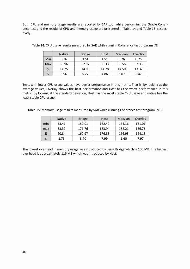
35

Both CPU and memory usage results are reported by SAR tool while performing the Oracle Coher-ence test and the results of CPU and memory usage are presented in Table 14 and Table 15, respec-tively.

Table 14: CPU usage results measured by SAR while running Coherence test program (%)

Native Bridge Host Macvlan Overlay

Min 0.76 3.54 1.51 0.76 0.75

Max 55.96 57.97 56.33 56.56 57.33

14.25 14.06 14.78 14.50 13.37

S 5.96 5.27 4.86 5.07 5.47

Tests with lower CPU usage values have better performance in this metric. That is, by looking at the average values, Overlay shows the best performance and Host has the worst performance in this metric. By looking at the standard deviation, Host has the most stable CPU usage and native has the least stable CPU usage.

Table 15: Memory usage results measured by SAR while running Coherence test program (MB)

Native Bridge Host Macvlan Overlay

min 53.41 152.01 162.49 164.16 161.01

max 63.39 171.76 183.94 168.21 166.76

60.84 160.97 176.88 166.93 164.13

s 1.73 8.70 7.99 1.60 7.97

The lowest overhead in memory usage was introduced by using Bridge which is 100 MB. The highest overhead is approximately 116 MB which was introduced by Host.

36

6. Discussion

6.1 Results

The jitter result of Macvlan is an interesting result to discuss since it is lower than the jitter of native. Although we could not find the cause of this improvement in jitter metric, but it is not uncommon that dockerized deployments outperform native deployments sometimes. For example, in [14] Macvlan showed lower network latency than native. Although in [14] the jitter was higher than na-tive, but the sample standard deviation for latency of Macvlan was lower than the native. Since jitter is the variation of delay and standard deviation of latency is also a calculation for variation in latency, then they are relevant. That is, the latency result for Macvlan in [14] was more stable than the one for native. Hence, seeing a jitter that is better than native is not something unexpected.

Moreover, the jitter results of Macvlan are more stable than the native according to the standard deviations. This result was not unexpected because other studies showed similar results such as [14]. Jitter buffers are usually used to counter the effect of the jitter. Since the jitter of Macvlan is predict-able, this means the size of jitter buffer required is predictable too.

Similarly, low latency overhead by Macvlan was expected since it was described as a driver with min-imum overhead [11]. In addition, similar results were obtained previously [14]. On the other hand, the overhead of 22.2% introduced by Overlay was matching with our expectations because of the encapsulation of container traffic in VXLAN packets [30].

When it comes to throughput, the results were interesting. All Docker networks showed more stable results than the native which is concluded from s. It is also interesting to see that both Host and Macvlan improved the throughput. It is not clear whether the use of Docker or the use of the unde-laying Linux virtual networks positively impacted the throughput and its stability. It is worth mention-ing that the theoretical maximum throughput is 12.5 MB/s because the hardware used is 100 Mbps and each byte is 8 bits. This theoretical maximum does not count for the overhead introduced by headers and trailers. The empirical results varied from 10.7 MB/s to 11.4 MB/s which are close to the theoretical limit after considering the headers and trailers of the packets. Overlay resulted in the lowest throughout of 10.7 MB/s. Overlay uses VXLAN encapsulation which forced us to reduce the packet size from 1486 to 1418 bytes. This in turn reduced the payload of each packet sent with Over-lay by 60 bytes. Therefore, the degradation of network throughput was expected for Overlay.

The error rate for native and all Docker networks except Overlay is 0.441% which is acceptable low rate. However, Docker Overlay network shows a huge error rate of 42.568%, which is ridiculously high. By inspecting the network statistics of SAR tool, we found that when using Overlay, Datagram Test Utility has caused a huge spike in network utilization in the begging of the test. This spike is around 3000 MB/s and it lasted for 1 second then disappeared. 3000 MB/s is few hundred times more than the hardware network capacity of 12.5 MB/s. The vast majority (or maybe all) of these packets were lost because of the hardware limitation. However, Datagram Test Utility counted them as lost packets and they negatively impacted the error rate. The same spike is repeated in all the three tests of Datagram Test Utility using Overlay. On the other hand, this spike is absent from the tests of all other networking modes. Thus, it seems that the actual error rate is much smaller than the result showed by Datagram Test Utility but the presence of the spike prevented the utility from showing the actual error rate. The high throughput of Overlay is evidence that the reported error rate is exaggerated and inaccurate since with this error rate or 42% the throughput should be signifi-cantly lower.

CPU usage results while running both Datagram Test Utility and Oracle Coherence showed that the CPU usage is similar in all Docker networks with native. The difference is expected to be even less when running on a system with powerful CPU with many cores. This is also something expected since [22] showed the effect of using Docker on CPU is negligible.

37

Memory usage was measured both while running Datagram Test Utility and Oracle Coherence test. The test memory usage was 35 MB and 61 MB for native in Datagram Test Utility and Oracle Coher-ence test, respectively. That is, the difference between the two tests in memory usage is 26 MB. On the other hand, the difference in memory usage between the two tests for each Docker network ranges between 10 MB and 50 MB. That is, Oracle Coherence test ran natively used 74% more memory than Datagram Test Utility in native. However, this percentage is not applicable for Docker networks. That suggests that the memory overhead introduced by Docker is not growing linearly with the application size. In fact, it does not seem to be growing at all. Further study is needed to confirm this finding.

The Oracle Coherence test program results showed that using Docker with Host network increased the total number of object put into the cluster by approximately 9.9%. Similarly, Macvlan network increased the total number of object put into the cluster by 6.6%. If we compare the ranking in this test with the ranking in the throughput test we find out that they are the same. That is, Host is the best, then Macvlan, then native, then Bridge, and finally Overlay. It was expected that throughput has a large impact on Oracle Coherence test since the two major reported parameters reported in Datagram Test Utility is the throughput and error rate. Given that Datagram Test Utility is the official tool provided by Oracle to test the network performance to tune it for Coherence. Since the error rate was the same for all Docker networks (except Overlay) and native, then throughput is the only dominant factor. However, the performance change in percentage is not the same between Data-gram Test Utility and Oracle Coherence test. Table 16 shows the average performance change com-pared to native in Datagram Test Utility and Oracle Coherence test.

Table 16: Performance comparison between throughput and Oracle Coherence test

Host Macvlan Native Bridge Overlay

Throughput (Datagram Test Utility) 0.3% 0.1% 0% -2.4% -5.4%

Oracle Coherence 9.9% 6.6% 0% -2.1% -12.1%

By looking at the comparison we can conclude that throughput is not the only factor in our case since the relative results from the two tests do not match. In fact, it looks like throughput is not the major contributor to the result and it seems that there are other dominant factors. Therefore, jitter and latency are expected to be contributing to these results more than the throughput. It is likely that latency and jitter contribution is higher than the throughput due to the unsaturated network traffic during the tests. It is expected that the throughput along with error rate to be dominant once the network traffic gets saturated.

We noticed also that native showed lowest standard deviation, i.e. most stable results, compared to Docker networks. On the contrary, the results of both Bridge and Host networks were the least sta-ble.

6.1.1 Overlay network packet size

Interesting results from Netperf, Datagram Test Utility, and SAR for overlay with packet size of 1468 bytes are presented Appendix B. The latency results from Netperf show a significant overhead of 49.3% to native compared to 22.2% only by Overlay with packet size of 1418 bytes. Datagram Test Utility shows a reduced throughput by 44.2% compared to 5.4% only by Overlay with packet size of 1418 bytes. SAR shows an increase of CPU usage from 17.30% in Overlay with packer size of 1418 bytes to 31.34% in Overlay with packet size of 1468 bytes. Remember that the Raspberry Pi used in this work use quad-core CPU, and the SAR tool display the average usage of all cores. At first glance, there seems no bottleneck causing this reduction in network throughput. However, when we in-

38

spected the individual core usage reported by SAR, we found that the CPU1 is saturated at 100% dur-ing the test and the other cores usage is significantly lower. So, the CPU is actually the bottleneck for the network performance given that the load is unevenly distributed between the cores. Other re-searches such as [31] also found this issue of CPU usage saturation due to datagram fragmentation. By inspecting the details of network interface inside Docker containers we found that except for Overlay the default MTU is 1500 bytes and it is 1450 bytes for Overlay interface because of the extra VXLAN header. When we use a packet size of 1468 bytes which is already exceeding the maximum MTU of 1450 bytes, fragmentation will take place at L2. On the receiver side, all received traffic will be defragmented. The process of fragmentation and defragmentation for all traffic is a CPU-hungry operation. Therefore, when we performed the throughput test for Overlay with packet size larger than the MTU the CPU usage increased and became a bottleneck for network performance.

6.2 Method

The method used in this work which is running tests on a system and measuring the performance is a common method used in many papers such as [14], [22], [23], and [21]. Similarly, the tools used in this work are also widely used in scientific papers and researches. The exception is being the Oracle Coherence test program which was developed specially for this thesis since there is no other tool allowed us to test the overall performance of Oracle Coherence cluster.

Validity of the results was achieved by using reliable tools for the measurement that are widely used in researches. Moreover, the same hardware and software environment was maintained during all tests. No other processes were running beside those which are necessary for the test in order to min-imize the noise and variations in the results.

Repeatability of the tests was verified by running each test at least three times. In the event that a test showed totally abnormal results then that particular test was considered as invalid and a re-placement test was performed.

Replicability of the results is possible by following the method described in the Method chapter. We tried to include all relevant and necessary information that simplify the process of replicating this work.

However, in this work we used a scaled down system that represents the actual system of geo-redundant data center. This simplification of the problem may have resulted in omitting part of the real system that is affected by different setups. If it have been possible, then studying the real system would have showed more accurate results of different setups on the system.

The use of Raspberry Pi devices can be replaced with powerful systems with large memory that is typically used when running in-memory data grid cluster. This can allow us to emulate the situation where we have multiple containers in each host and a Coherence node running inside each contain-er. This can show us how each metric respond to scaling up the number of nodes and traffic generat-ed.

The method we used to evaluate the performance of Oracle Coherence was by running a test pro-gram that consciously performs put operation on the cluster for a specific period. The cluster size in this work is two nodes and only one of them has storage enabled. This method was chosen because of its simplicity and it simulates a real cluster with continuous operations involving network traffic. This method provided us with a controlled environment that allowed us to easily perform the test and the measurement. However, in real scenario the cluster consist of more nodes with multiple nodes having enables storage. This means that the data is not flowing always to the same node be-cause it is not the only node with enabled storage. In addition, the distributed cache algorithm will involve distributing and updating data among the nodes with enabled storage which is not applicable when there is only a single node with enabled storage. Moreover, higher number of nodes is likely to have higher utilization of the network bandwidth which may lead results to be more throughput-

39

oriented. These are some of the aspects that were simplified in the test program but they exist in the real system.

In this work, we used some peer-reviewed papers that are well-cited such as [22] and [23]. However, the best source for reliable technical information for Oracle Coherence is the official website. Similar-ly, Docker official website is the most reliable and updated source for getting necessary technical information related to Docker. The same is applied when we wanted to get technical information about the measurement tools used. That is, the main sources used in this work are peer-reviewed papers and official websites.

40

7. Conclusion

The aim of this work is to find the impact of Docker networking on performance metrics in general and particularly for data grid systems. This was achieved by running different tests on a scaled down version of a real system to measure various performance metrics. The results obtained were analyzed and compared to native deployment. The results show that the performance is affected by Docker networking and the details are presented in the results chapter.

7.1 Answering research question

The research questions presented in ‎1.3 are answered throughout the report, but we revisit them here and summarize the answers to these questions.

What is the effect of different Docker network drivers on various performance metrics?

For network performance metrics in general, Host and Macvlan networks showed a perfor-mance that is similar to native. Bridge performance is slightly lower than native and Overlay introduced a considerable overhead. CPU performance metric was not much different be-tween the networking modes. Memory usage metric showed small differences between dif-ferent Docker networks, except Bridge which showed a lower memory usage. The detailed results answering this question are presented in ‎5.1, ‎5.2, ‎5.3, and ‎5.4.

What is the effect of different Docker network drivers on the performance of a dockerized in-memory data grid system?

The overall cluster performance showed that Host network performs 9.9% better than native and similarly Macvlan performs 6.6% better than native. Bridge overhead introduced a per-formance reduction of 2.1% and Overlay introduced a reduction in performance of 12.1%. CPU usage metric did not show a considerable different between the networking modes. In memory usage metric, no big difference was shown in the results between Docker networks. The detailed results answering this question are presented in ‎5.5.

What is the performance difference between native and dockerized distributed data grid system?

As detailed in the previous question, both Host and Macvlan improved the cluster perfor-mance while Bridge resulted in slight overhead. Dockerizing the data grid system and using Overlay network caused a significant performance reduction of 12.1% compared to native. CPU usage metric of all Docker networking modes compared to native is very similar. The memory usage overhead of dockerizing the data grid system varies between approximately 100 MB and 106 MB. The detailed results answering this question are presented in ‎5.5.

7.2 Considerations when selecting a networking mode

When it comes to choosing a networking mode for a real system then there are other aspects that need to be considered along with the performance such as security, usability, complexity, and availa-bility.

Looking at the Coherence test results for Host network we find that there is a considerable perfor-mance gain. However, this networking mode has its drawbacks. A major disadvantage of using Host network is that the container will have access to all network interfaces of the host machine and be able to communicate with all machines and even containers that the host can communicate with.

Macvlan results are good and show a performance gain also compared to native. However, to get the full use of Macvlan it needs to be combined with the use of VLANs. The reason is that each container will have its own MAC address and consequently IP address. Packets with MAC addresses that belong to containers will be flowing over physical network. Therefore, the physical network needs to be con-

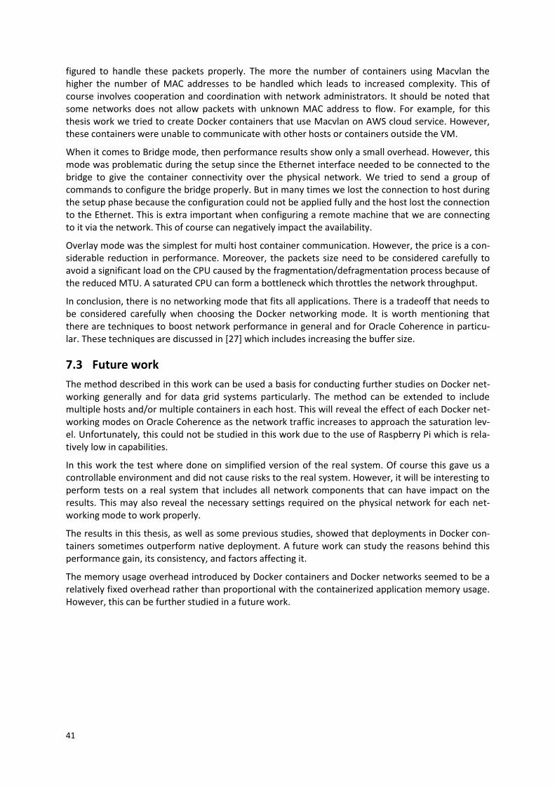
41

figured to handle these packets properly. The more the number of containers using Macvlan the higher the number of MAC addresses to be handled which leads to increased complexity. This of course involves cooperation and coordination with network administrators. It should be noted that some networks does not allow packets with unknown MAC address to flow. For example, for this thesis work we tried to create Docker containers that use Macvlan on AWS cloud service. However, these containers were unable to communicate with other hosts or containers outside the VM.

When it comes to Bridge mode, then performance results show only a small overhead. However, this mode was problematic during the setup since the Ethernet interface needed to be connected to the bridge to give the container connectivity over the physical network. We tried to send a group of commands to configure the bridge properly. But in many times we lost the connection to host during the setup phase because the configuration could not be applied fully and the host lost the connection to the Ethernet. This is extra important when configuring a remote machine that we are connecting to it via the network. This of course can negatively impact the availability.

Overlay mode was the simplest for multi host container communication. However, the price is a con-siderable reduction in performance. Moreover, the packets size need to be considered carefully to avoid a significant load on the CPU caused by the fragmentation/defragmentation process because of the reduced MTU. A saturated CPU can form a bottleneck which throttles the network throughput.

In conclusion, there is no networking mode that fits all applications. There is a tradeoff that needs to be considered carefully when choosing the Docker networking mode. It is worth mentioning that there are techniques to boost network performance in general and for Oracle Coherence in particu-lar. These techniques are discussed in [27] which includes increasing the buffer size.

7.3 Future work

The method described in this work can be used a basis for conducting further studies on Docker net-working generally and for data grid systems particularly. The method can be extended to include multiple hosts and/or multiple containers in each host. This will reveal the effect of each Docker net-working modes on Oracle Coherence as the network traffic increases to approach the saturation lev-el. Unfortunately, this could not be studied in this work due to the use of Raspberry Pi which is rela-tively low in capabilities.

In this work the test where done on simplified version of the real system. Of course this gave us a controllable environment and did not cause risks to the real system. However, it will be interesting to perform tests on a real system that includes all network components that can have impact on the results. This may also reveal the necessary settings required on the physical network for each net-working mode to work properly.

The results in this thesis, as well as some previous studies, showed that deployments in Docker con-tainers sometimes outperform native deployment. A future work can study the reasons behind this performance gain, its consistency, and factors affecting it.

The memory usage overhead introduced by Docker containers and Docker networks seemed to be a relatively fixed overhead rather than proportional with the containerized application memory usage. However, this can be further studied in a future work.

42

Reference List

[1] A. Mouat, Using Docker, 1st ed. Sebastopol: O’Reilly Media Inc., 2015. [2] “Defining a Data Grid.” [Online]. Available:

https://docs.oracle.com/cd/E14526_01/coh.350/e14510/definingdatagrid.htm. [Accessed: 10-Aug-2017].

[3] “Introduction to Coherence Caches.” [Online]. Available: https://docs.oracle.com/middleware/12212/coherence/develop-applications/introduction-coherence-caches.htm. [Accessed: 10-Aug-2017].

[4] “Introduction to Coherence.” [Online]. Available: https://docs.oracle.com/middleware/12212/coherence/develop-applications/introduction-coherence.htm. [Accessed: 10-Aug-2017].

[5] “Raspberry Pi FAQs - Frequently Asked Questions.” [Online]. Available: https://www.raspberrypi.org/help/faqs/. [Accessed: 25-May-2017].

[6] “Docker Machine Overview | Docker Documentation.” [Online]. Available: https://docs.docker.com/machine/overview/. [Accessed: 02-Jun-2017].

[7] “Docker.” [Online]. Available: http://delftswa.github.io/chapters/docker/. [Accessed: 02-Apr-2017].

[8] “About images, containers, and storage drivers | Docker Documentation.” [Online]. Available: https://docs.docker.com/engine/userguide/storagedriver/imagesandcontainers/. [Accessed: 02-Jun-2017].

[9] “Docker Overview - Docker Documentation.” [Online]. Available: https://docs.docker.com/engine/understanding-docker/. [Accessed: 02-Apr-2017].

[10] R. Dua et al., Learning Docker networking: become a proficient Linux administrator by learning the art of container networking with elevated efficiency using Docker. Switzerland, Europe: Packt Publ., 2016.

[11] M. Church, “Docker Reference Architecture: Designing Scalable, Portable Docker Container Networks - Docker, Inc.,” 2016. [Online]. Available: https://success.docker.com/Architecture/Docker_Reference_Architecture%3A_Designing_Scalable%2C_Portable_Docker_Container_Networks. [Accessed: 01-Apr-2017].

[12] M. Mahalingam et al., “Virtual eXtensible Local Area Network (VXLAN): A Framework for Overlaying Virtualized Layer 2 Networks over Layer 3 Networks.” [Online]. Available: https://www.ietf.org/rfc/rfc7348.txt. [Accessed: 01-Jun-2017].

[13] “Bridge vs Macvlan – HiCube.” [Online]. Available: https://hicu.be/bridge-vs-macvlan. [Accessed: 02-Jun-2017].

[14] J. Anderson et al., “Performance Considerations of Network Functions Virtualization using Containers,” in Proc. 2016 International Conference on Computing, Networking and Communications (ICNC), 2016, pp. 1–7.

[15] S. Bradner and J. McQuaid, “Benchmarking Methodology for Network Interconnect Devices,” RFC2544, 1999. [Online]. Available: https://www.ietf.org/rfc/rfc2544.txt. [Accessed: 27-Mar-2017].

[16] N. Spring et al., “Using PlanetLab for Network Research: Myths, Realities, and Best Practices,” SIGOPS Oper. Syst. Rev., vol. 40, no. 1, pp. 17–24, Jan. 2006.

[17] J. Whiteaker et al., “Explaining Packet Delays Under Virtualization,” SIGCOMM Comput. Commun. Rev., vol. 41, no. 1, pp. 38–44, Jan. 2011.

[18] H. Schulzrinne et al., “RTP: A Transport Protocol for Real-Time Applications,” RFC3550, 2003. [Online]. Available: https://www.ietf.org/rfc/rfc3550.txt. [Accessed: 27-Mar-2017].

[19] N. Regola and J. C. Ducom, “Recommendations for Virtualization Technologies in High Performance Computing,” in Proc. 2010 IEEE Second International Conference on Cloud Computing Technology and Science, 2010, pp. 409–416.

[20] E. Kohler et al., “The Click Modular Router,” ACM Trans. Comput. Syst., vol. 18, no. 3, pp. 263–

43

297, Aug. 2000. [21] F. Ramalho and A. Neto, “Virtualization at the network edge: A performance comparison,” in

Proc. 2016 IEEE 17th International Symposium on A World of Wireless, Mobile and Multimedia Networks (WoWMoM), 2016, pp. 1–6.

[22] W. Felter et al., “An updated performance comparison of virtual machines and Linux containers,” in Proc. 2015 IEEE International Symposium on Performance Analysis of Systems and Software (ISPASS), 2015, pp. 171–172.

[23] R. Morabito et al., “Hypervisors vs. Lightweight Virtualization: A Performance Comparison,” in Proc. 2015 IEEE International Conference on Cloud Engineering, 2015, pp. 386–393.

[24] “SYSSTAT.” [Online]. Available: http://sebastien.godard.pagesperso-orange.fr/man_sar.html. [Accessed: 10-May-2017].

[25] “Performing a Datagram Test for Network Performance.” [Online]. Available: http://docs.oracle.com/cd/E14526_01/coh.350/e14509/datagramtest.htm. [Accessed: 16-May-2017].

[26] “Performing a Network Performance Test.” [Online]. Available: https://docs.oracle.com/middleware/12212/coherence/administer/performing-network-performance-test.htm. [Accessed: 08-Jun-2017].

[27] “Performance Tuning.” [Online]. Available: https://docs.oracle.com/middleware/12212/coherence/administer/performance-tuning.htm. [Accessed: 08-Jun-2017].

[28] B. Borges, “Oracle Coherence Docker Image,” 2016. [Online]. Available: https://github.com/oracle/docker-images/tree/master/OracleCoherence. [Accessed: 31-Mar-2017].

[29] “IBM Knowledge Center - Running Netperf UDP request response test.” [Online]. Available: https://www.ibm.com/support/knowledgecenter/en/SSQPD3_2.4.0/com.ibm.wllm.doc/runnetperf.html. [Accessed: 17-May-2017].

[30] J. Weerasinghe and F. Abel, “On the Cost of Tunnel Endpoint Processing in Overlay Virtual Networks,” in Proc. 2014 IEEE/ACM 7th International Conference on Utility and Cloud Computing, 2014, pp. 756–761.

[31] A. Zismer, “Performance of Docker Overlay Networks,” University of Amsterdam, 2016.

44

Appendix A: Oracle Coherence Test Program

import com.tangosol.net.CacheFactory; import com.tangosol.net.NamedCache; import org.apache.commons.lang3.RandomStringUtils; import java.util.Random; import java.util.Date; import java.text.DateFormat; import java.text.SimpleDateFormat; public class ClusterTest { public static void main(String[] args) { DateFormat dateFormat = new SimpleDateFormat("yyyy/MM/dd HH:mm:ss"); Date date = new Date(); System.out.println("Starting time of test: " + dateFormat.format(date)); CacheFactory.ensureCluster(); NamedCache<Object, Object> cache = CacheFactory.getCache("hello-example"); String value1 = RandomStringUtils.randomAlphanumeric(700); long startTime = System.currentTimeMillis(); long elapsedTime = 0; int i = 0; int testTime = 5*60*1000; while (elapsedTime < testTime) { cache.remove("k"+i++); cache.put("k"+i, value1); elapsedTime = (new Date()).getTime() - startTime; } if (cache.get("k"+i) != null) System.out.println("Total objects added to the cluster: " + i); CacheFactory.shutdown(); } }

45

Appendix B: Results for Overlay (1468 Bytes Packets)

Table 17: 1-way latency results of Overlay with packet size of 1468 bytes measured by Netperf (ms)

1-way latency

min 0.752

max 0.767

0.761

s 0.008

Table 18: Throughput results for overlay network with packet size of 1468 bytes (MB/s)

Throughput (MB/s) CPU usage (%) Memory usage (MB)

min 6.021 28.42 154.89

max 6.817 55.06 319.43

6.336 31.34 215.78

s 0.327 2.12 72.72

Table 19: Detailed throughput, error rate, CPU usage, and memory usage results for overlay network with packet size of 1468 bytes

Duration (ms)

Throughput (MB/sec)

Throughput (packets/sec)

Missing packets

Success rate (%)

CPU usage (%)

Memory usage (MB)

Test 1

min 22112 6.021 4301 44481 0.31352 29.35 310.07

max 23250 6.331 4522 218956 0.69213 50.76 319.43

22532 6.214 4439 170955 0.39209 31.47 317.85

s 247 0.067 48 56665 0.11767 1.88 3.38

Total 495705 n/a n/a 3761018 n/a n/a n/a

Test 2

min 21034 6.166 4404 35091 0.33062 28.91 165.51

max 22708 6.656 4754 202458 0.74024 53.27 183.15

21875 6.401 4572 173384 0.37853 31.16 173.92

s 324 0.095 68 41229 0.09128 2.07 6.34

Total 481254 n/a n/a 3814453 n/a n/a n/a

Test 3

min 20536 6.236 4454 37277 0.33074 28.42 154.89

max 22451 6.817 4869 202353 0.72845 55.06 155.81

21914 6.392 4566 128285 0.48571 31.38483 155.57

s 517 0.155 111 68503 0.16861 2.37788 0.36

Total 482107 n/a n/a 2822274 n/a n/a n/a

46

Appendix C: Detailed Results of Datagram Test Utility

Table 20: Throughput, error rate, CPU usage, and memory usage results for native setup

Duration (ms)

Throughput (MB/sec)

Throughput (packets/sec)

Missing packets

Success rate (%)

CPU usage (%)

Memory usage (MB)

Test 1

min 12262 11.332 8094 0 0.99743 8.33 33.73

max 12355 11.417 8155 258 1.00000 38.53 35.57

12277 11.403 8145 45 0.99956 16.30 34.97

s 20 0.0180 13 74 0.00073 4.29 0.86

Total 270096 n/a n/a 980 n/a n/a n/a

Test 2

min 12257 9.177 6555 0 0.81127 10.40 32.18

max 15255 11.423 8159 23264 1.00000 42.35 37.93

12457 11.263 8045 1350 0.98859 16.39 35.66

s 646 0.488 349 4991 0.04069 4.70 2.27

Total 274063 n/a n/a 29701 n/a n/a n/a

Test 3

min 12260 11.127 7948 0 0.97745 9.48 30.18

max 12582 11.420 8157 2307 1.00000 45.09 36.27

12282 11.399 8142 141 0.99862 15.53 35.01

s 67 0.061 44 488 0.00477 5.03 1.39

Total 270213 n/a n/a 3095 n/a n/a n/a

Table 21: Throughput, error rate, CPU usage, and memory usage results for Docker bridge network

Duration (ms)

Throughput (MB/sec)

Throughput (packets/sec)

Missing packets

Success rate (%)

CPU usage (%)

Memory usage (MB)

Test 1

min 12256 10.651 7608 0 0.94816 11.76 111.13

max 13144 11.423 8159 5467 1.00000 59.15 154.36

12683 11.043 7888 416 0.99599 17.94 113.13

s 257 0.222 159 1194 0.01135 5.61 8.24

Total 279026 n/a n/a 9154 n/a n/a n/a

Test 2

min 12259 10.608 7577 73066 0.43016 11.76 103.57

max 13197 11.4120 8157 132471 0.57781 49.42 147.67

12606 11.110 7936 120910 0.45428 17.91 106.47

s 270 0.236 168 12302 0.03032 5.51 8.25

Total 277335 n/a n/a 2660021 n/a n/a n/a

Test 3

min 12262 10.504 7503 50200 0.42850 11.07 111.05

47

max 13328 11.417 8155 133373 0.66578 44.88 153.84

12619 11.101 7929 116674 0.46629 17.97 113.35

s 307 0.267 191 19541 0.05556 5.59 8.12

Total 277608 n/a n/a 2566833 n/a n/a n/a

Table 22: Throughput, error rate, CPU usage, and memory usage results for Docker host network

Duration (ms)

Throughput (MB/sec)

Throughput (packets/sec)

Missing packets

Success rate (%)

CPU usage (%)

Memory usage (MB)

Test 1

min 12260 11.263 8045 0 0.99380 10.19 146.74

max 12430 11.420 8157 624 1.00000 47.45 180.12

12280 11.401 8144 161 0.99840 19.31 166.63

s 37 0.034 24 139 0.00138 3.91 15.23

Total 270149 n/a n/a 3537 n/a n/a n/a

Test 2

min 12261 10.977 7841 0 0.95649 9.06 146.29

max 12753 11.418 8156 4549 1.00000 44.97 147.29

12303 11.380 8129 378 0.99632 18.17 146.38

s 114 0.103 73 967 0.00925 4.50 0.29

Total 270671 n/a n/a 8312 n/a n/a n/a

Test 3

min 12260 11.259 8042 0 0.99721 9.35 146.43

max 12435 11.420 8157 280 1.00000 46.35 148.53

12280 11.401 8144 106 0.99894 17.37 148.01

s 36 0.033 24 87 0.00087 4.82 0.46

Total 270152 n/a n/a 2333 n/a n/a n/a

Table 23: Throughput, error rate, CPU usage, and memory usage results for Docker Macvlan network

Duration (ms)

Throughput (MB/sec)

Throughput (packets/sec)

Missing packets

Success rate (%)

CPU usage (%)

Memory usage (MB)

Test 1

min 12265 10.867 7762 0 0.94816 10.19 153.63

max 12883 11.414 8153 5467 1.00000 51.84 168.73

12331 11.355 8111 416 0.99599 18.87 156.54

s 143 0.127 91 1194 0.01135 4.74 3.82

Total 271282 n/a n/a 9154 n/a n/a n/a

Test 2

min 12260 11.201 8001 0 0.98075 9.35 138.60

max 12498 11.420 8157 1963 1.00000 45.11 139.80

12285 11.396 8140 236 0.99766 19.41 139.77

s 56 0.051 36 407 0.00399 3.99 0.13

Total 270277 n/a n/a 5201 n/a n/a n/a

48

Test 3

min 12261 10.543 7531 0 0.93022 8.78 153.52

max 13278 11.418 8156 7502 1.00000 52.53 154.52

12335 11.353 8109 629 0.99401 18.58 153.52

s 229 0.198 141 1713 0.01602 4.68 0.06

Total 271379 n/a n/a 13846 n/a n/a n/a

Table 24: Throughput, error rate, CPU usage, and memory usage results for Docker overlay network

Duration (ms)

Throughput (MB/sec)

Throughput (packets/sec)

Missing packets

Success rate (%)

CPU usage (%)

Memory usage (MB)

Test 1

min 12256 10.006 7399 51924 0.51053 10.98 151.41

max 13516 11.034 8159 95875 0.65822 60.53 159.96

12790 10.585 7827 80067 0.55679 17.83 157.93

s 436 0.358 265 9053 0.03007 4.59 3.64

Total 281375 n/a n/a 1761478 n/a n/a n/a

Test 2

min 12259 9.802 7248 33832 0.51757 11.00 146.82

max 13796 11.031 8157 93211 0.74721 51.14 148.75

12581 10.757 7955 72957 0.58173 16.91 147.25

s 369 0.302 224 13015 0.04981 4.17 0.81

Total 276781 n/a n/a 1605047 n/a n/a n/a

Test 3

min 12257 10.245 7576 38633 0.53157 1.75 155.21

max 13199 11.034 8159 88121 0.72133 75.57 163.26

12446 10.871 8039 72324 0.58445 17.15 155.93

s 306 0.259 191 14022 0.05358 7.77 2.31

Total 273820 n/a n/a 1591128 n/a n/a n/a