The slides are from several sources through James Hays (Brown); Silvio Savarese (U. of Michigan); Bill Freeman and Antonio Torralba (MIT), including their own slides.

CLUSTERING SEGMENTATION

Basic ideas of grouping in human vision

• Figure-ground discrimination • Emergence

• Gestalt properties

Currently in computer vision we don't really take into account the top-down (from the "memory") grouping only the bottom-up part.

A series of factors affect whether elements should be grouped together. Difficult to translate into algorithms.

Gestalt properties Berlin School early 20th century

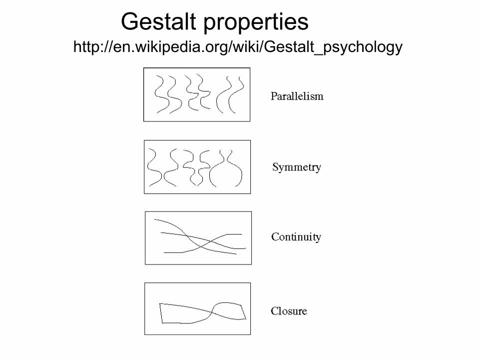
Gestalt properties http://en.wikipedia.org/wiki/Gestalt_psychology

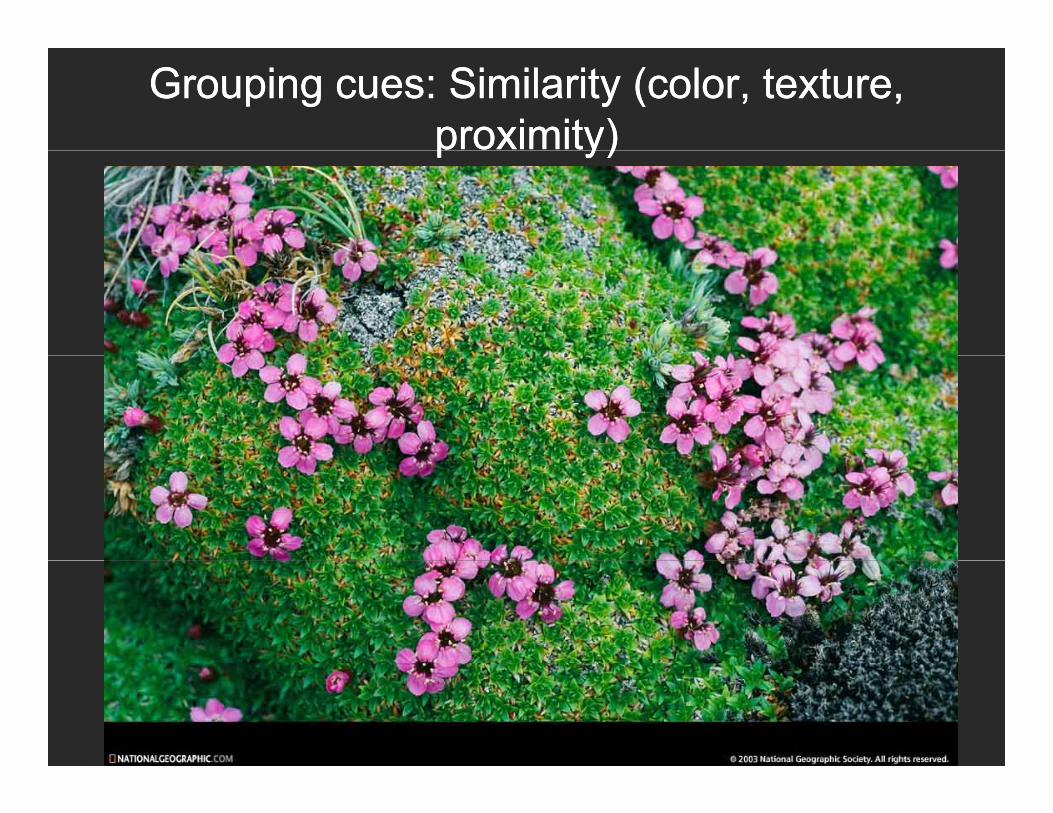
Grouping cues: Similarity (color, texture,Grouping cues: Similarity (color, texture,proximity)proximity)p y)p y)

Grouping cues: “Common fate”Grouping cues: “Common fate”

Image credit: Arthus-Bertrand (via F. Durand)

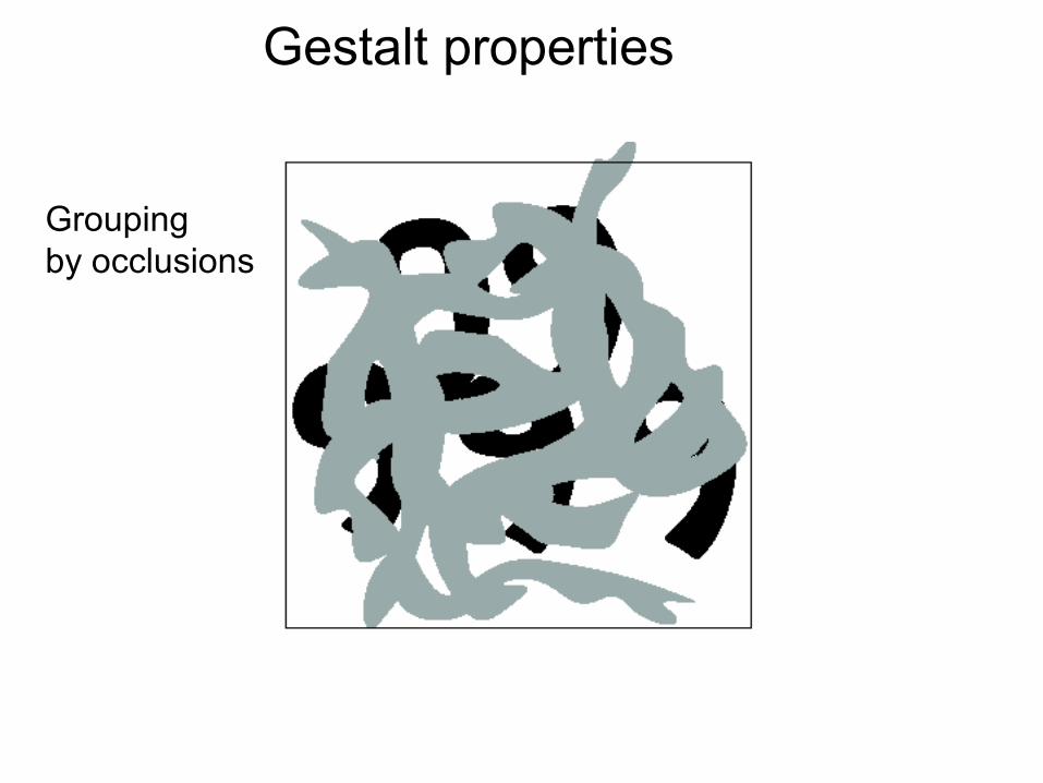
Gestalt properties

Grouping by occlusions

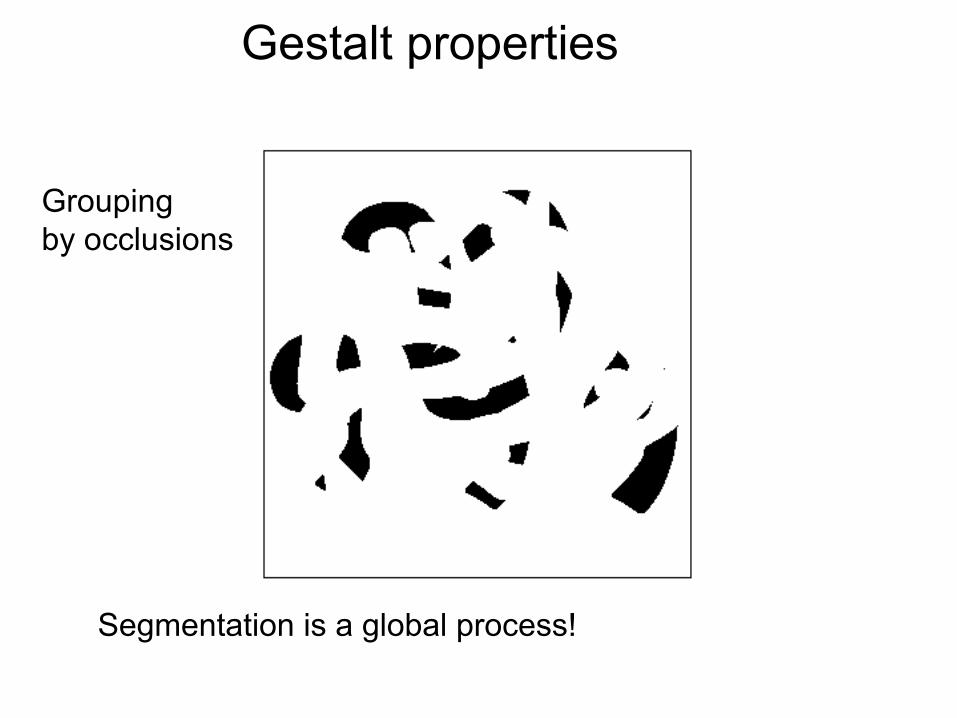
Gestalt properties

Grouping by occlusions

Segmentation is a global process!

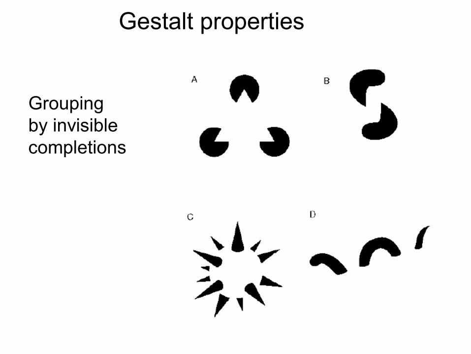
Gestalt properties

Grouping by invisible completions

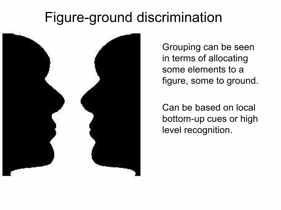
Grouping can be seen in terms of allocating some elements to a figure, some to ground.

Can be based on local bottom-up cues or high level recognition.

Figure-ground discrimination

Figure-ground discrimination

Emergence

1970s: R. C. James

2000s: Bev Doolittle

Emergence

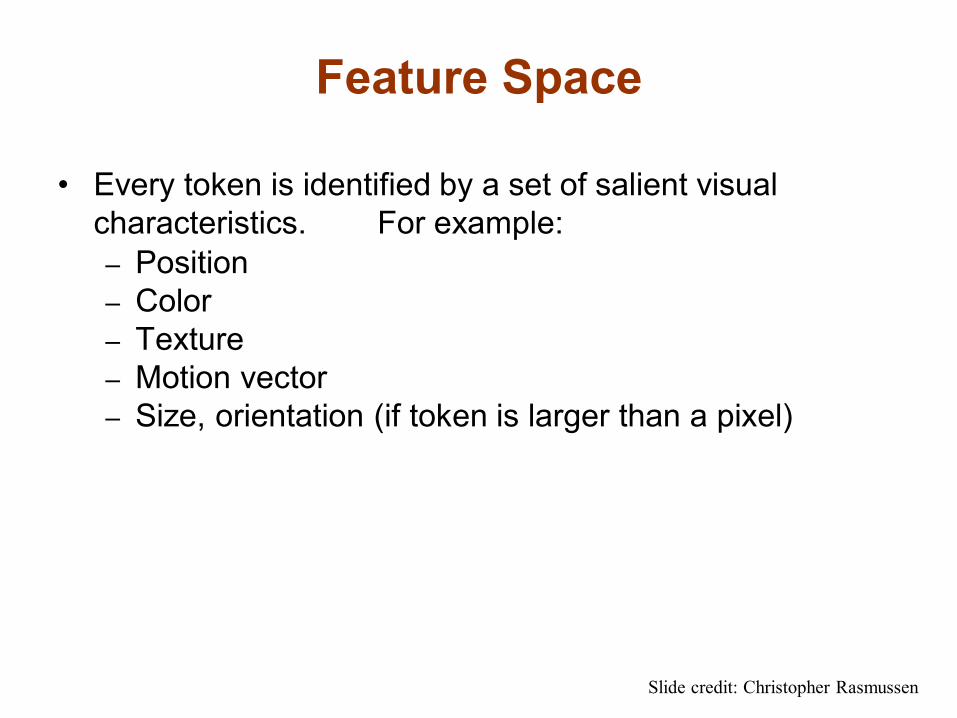
Feature Space

• Every token is identified by a set of salient visual characteristics. For example: – Position – Color – Texture – Motion vector – Size, orientation (if token is larger than a pixel)

Slide credit: Christopher Rasmussen

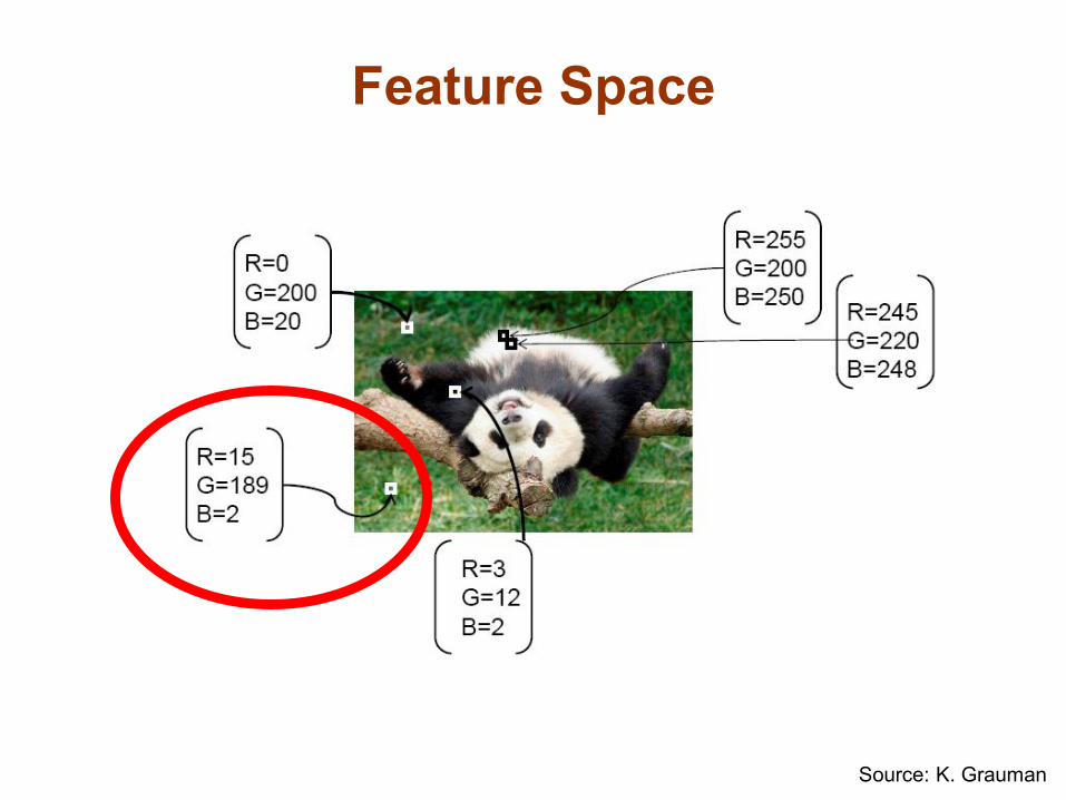
Source: K. Grauman

Feature Space

Feature space: each token is represented by a point.

r

b

g

r

b

g

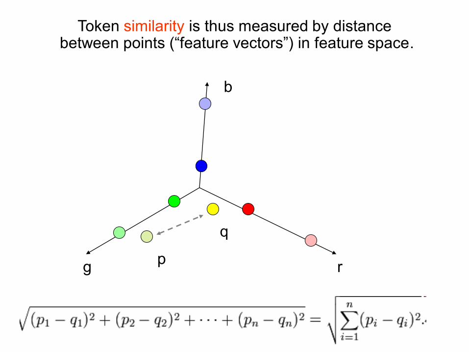
Token similarity is thus measured by distance between points (“feature vectors”) in feature space.

q

p

r

b

g

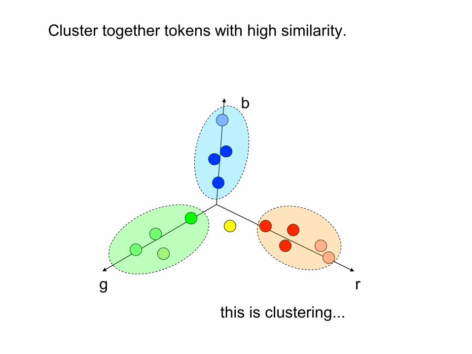
Cluster together tokens with high similarity.

this is clustering...

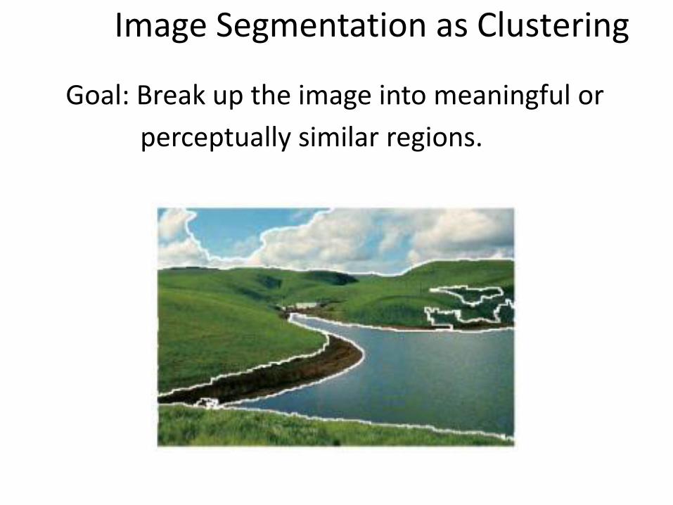
Image Segmentation as Clustering

Goal: Break up the image into meaningful or

perceptually similar regions.

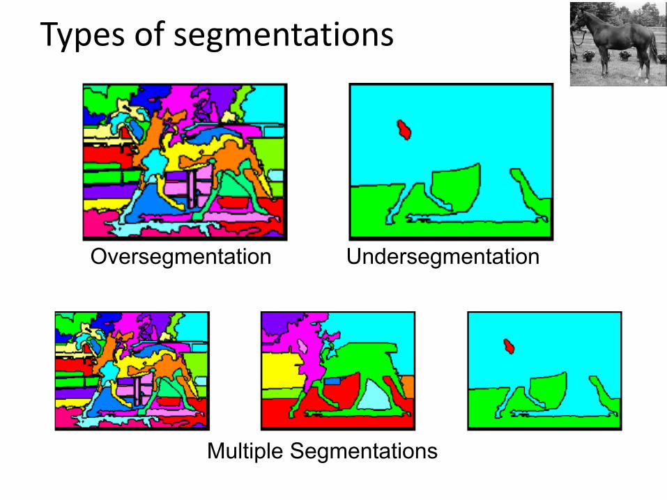
Types of segmentations

Oversegmentation Undersegmentation

Multiple Segmentations

Why do we cluster?

Summarizing large quantity of data in a few clusters with a few parameters. Each cluster can be used to predict if an unknown region becomes this cluster or not. Segmentation of an image (mainly those in 2D) can be achieved upto a decent estimate... usually.

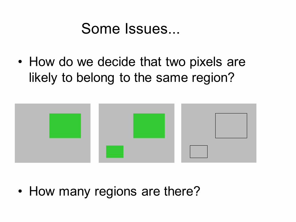
Some Issues...

• How do we decide that two pixels are likely to belong to the same region?

• How many regions are there?

Segmentation as clustering Cluster together tokens that share similar

visual characteristics.Will examine:

• K-mean • Mean-shift

Many other clustering methods exist, some using the graph structure of the image are also popular. But none of the clustering algorithm, as advancedas they are, can give a complete segmentationof the 3D reality in the 2D image.

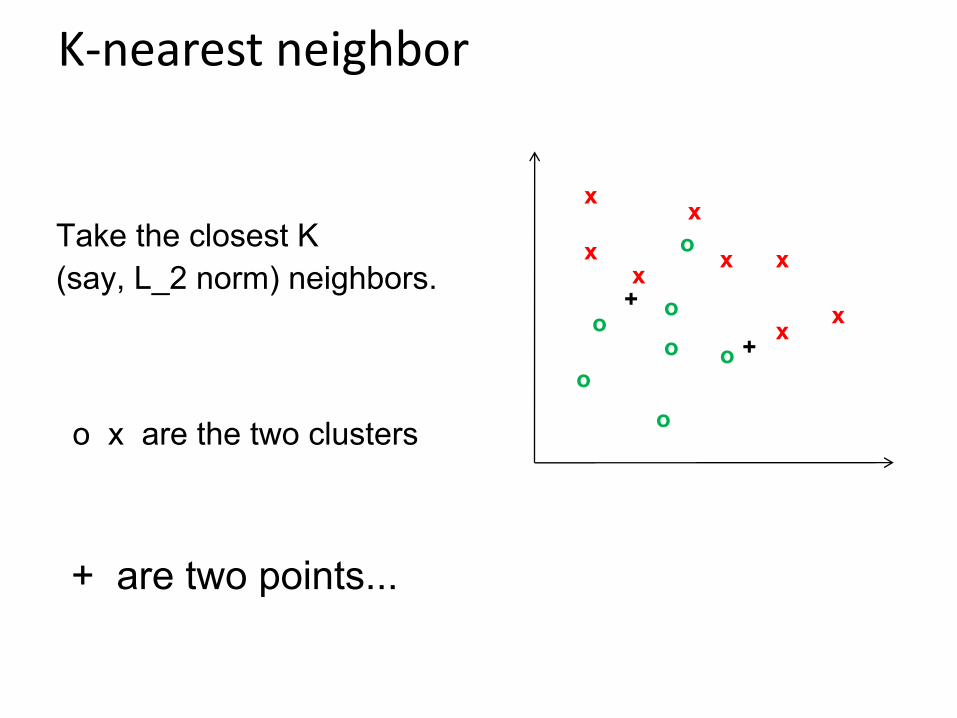
K-nearest neighbor

x x

x x

x

x x

x o

o o

o

o

o o

+

+

Take the closest K(say, L_2 norm) neighbors.

+ are two points...

o x are the two clusters

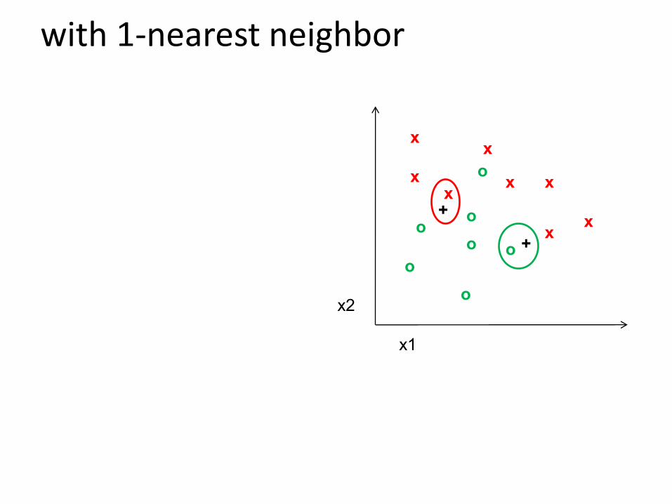
with 1-nearest neighbor

x x

x x

x

x x

x o

o o

o

o

o o

x2

x1

+

+

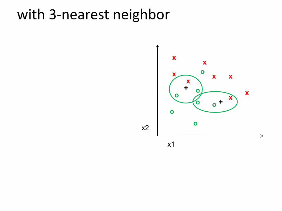
with 3-nearest neighbor

x x

x x

x

x x

x o

o o

o

o

o o

x2

x1

+

+

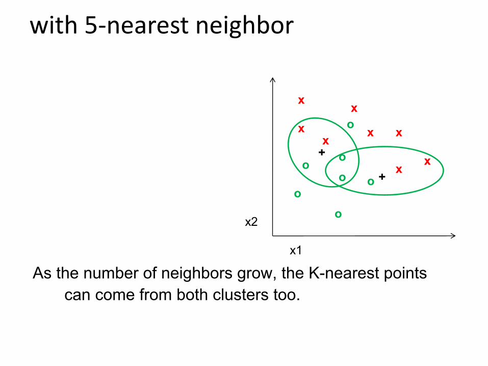
with 5-nearest neighbor

x x

x x

x

x x

x o

o o

o

o

o o

x2

x1

+

+

As the number of neighbors grow, the K-nearest points can come from both clusters too.

K-Means Clustering • Initialization:

Given K, number of clusters; N points in feature space. Pick K points randomly. These are initial cluster centers (means) 1, …, . Repeat the following:

Slide credit: Christopher Rasmussen

1. Assign each of the N points, xj , to clusters by nearest i.2. Recompute mean i of each cluster from its member points

3. If no mean has changed more than some , stop.

objective function

K

K

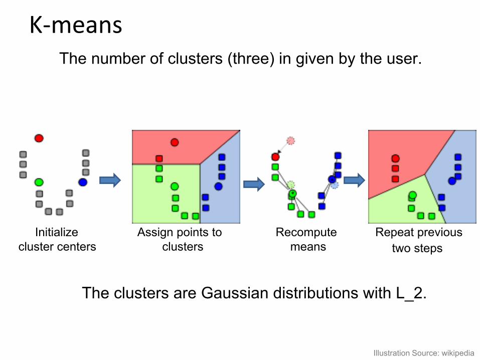
K-means

Illustration Source: wikipedia

Initialize cluster centers

Assign points to clusters

Recompute means

Repeat previous two steps

The number of clusters (three) in given by the user.

The clusters are Gaussian distributions with L_2.

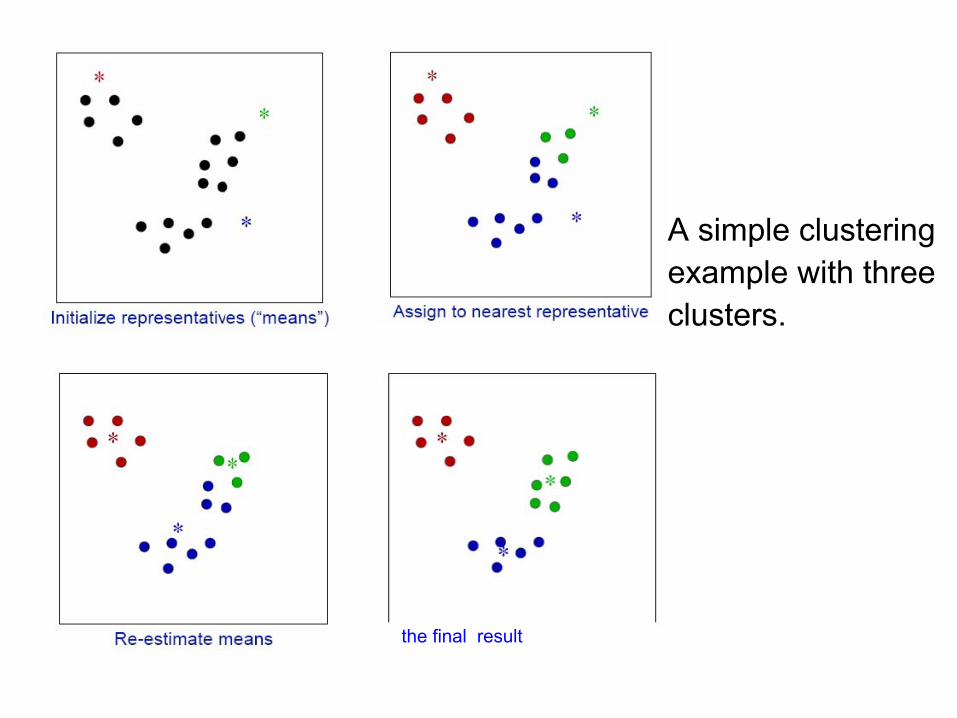
the final result

A simple clusteringexample with threeclusters.

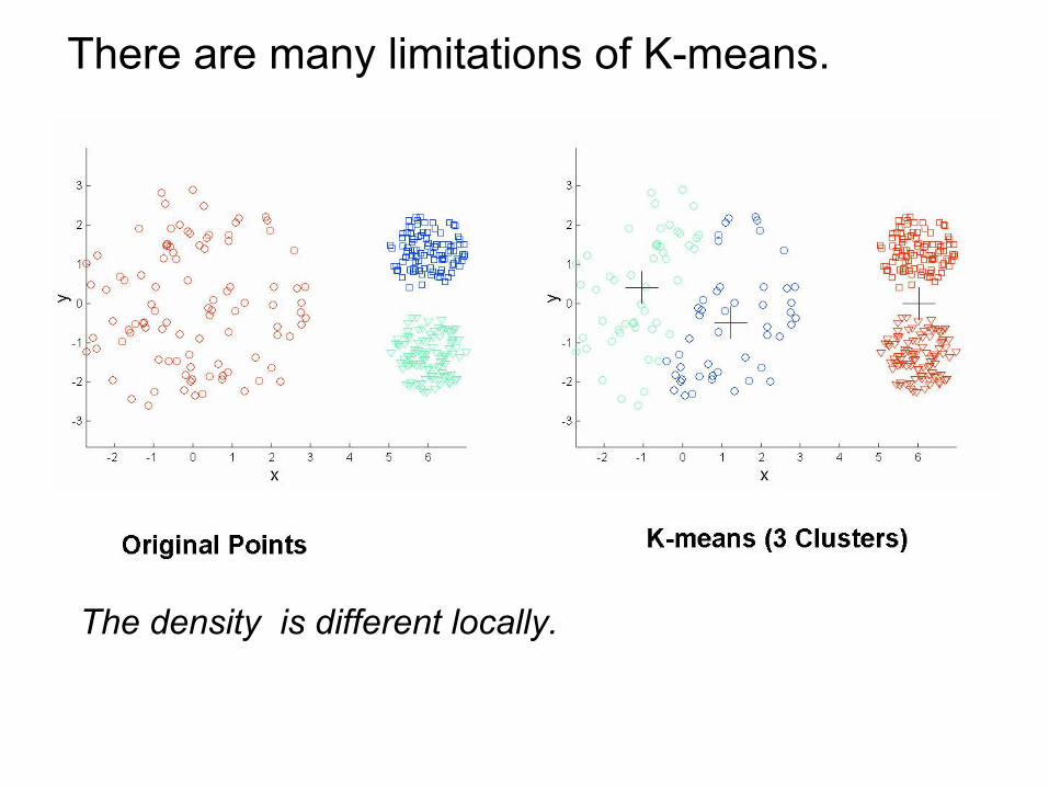
There are many limitations of K-means.

The density is different locally.

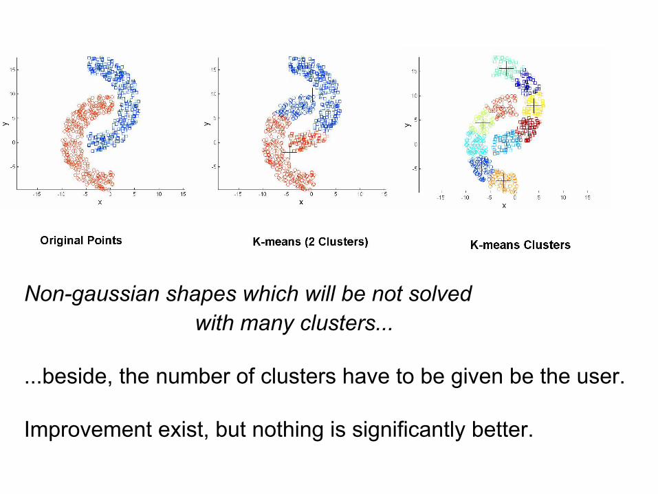
Non-gaussian shapes which will be not solved with many clusters...

...beside, the number of clusters have to be given be the user.

Improvement exist, but nothing is significantly better.

K-Means pros and cons

• Pros – Simple and fast. – Converges to a local minimum of the error function.

• Cons – Need to pick K. – Sensitive to initialization. – Only finds “spherical” clusters. – Sensitive to outliers.

Rarely used for segmentation.

adaptive?!

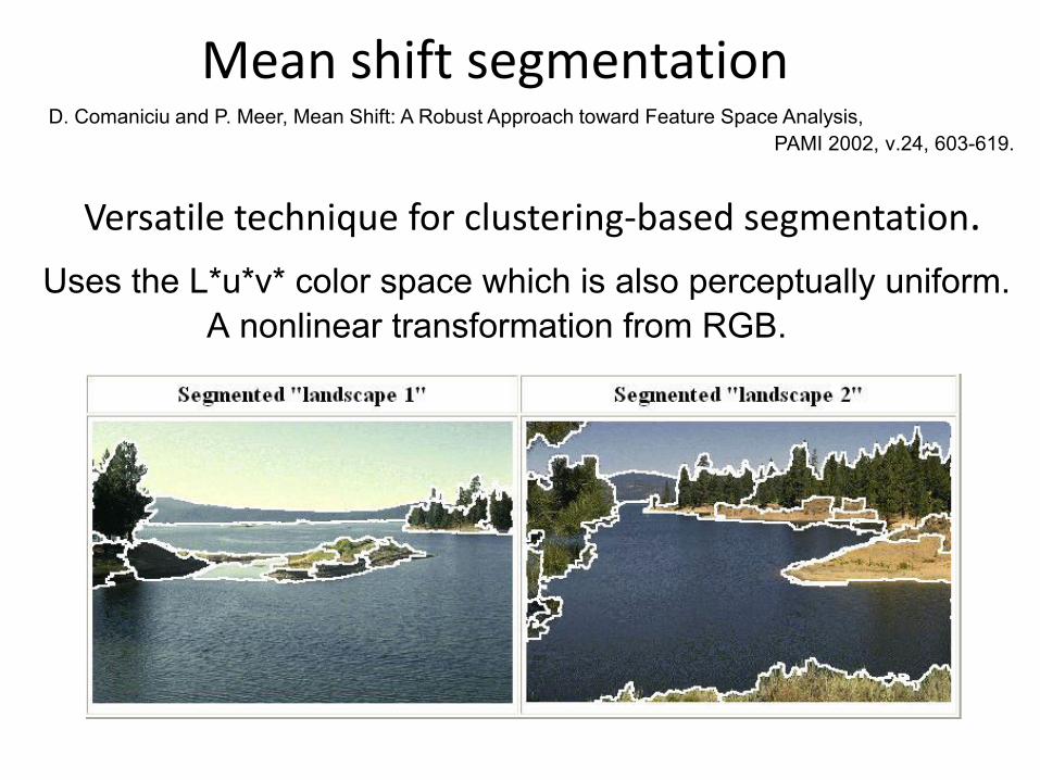
Versatile technique for clustering-based segmentation.

D. Comaniciu and P. Meer, Mean Shift: A Robust Approach toward Feature Space Analysis, PAMI 2002, v.24, 603-619.

Mean shift segmentation

Uses the L*u*v* color space which is also perceptually uniform. A nonlinear transformation from RGB.

Mean shift algorithm...

...try to find modes of this non-parametric density.

Kernel density estimation

Kernel density estimation function

K(x) > 0 only for ||x|| <= 1the bandwidth, h, has to be given by the user. The kernel is symmetric are depents on x . The Epanachikov kernel ~(1 - ||x|| )and the truncated Gaussian kernel

are used.

2

2

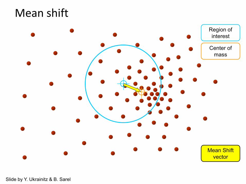
Region of interest

Center of mass

Mean Shift vector

Slide by Y. Ukrainitz & B. Sarel

Mean shift

Region of interest

Center of mass

Mean Shift vector

Slide by Y. Ukrainitz & B. Sarel

Mean shift

Region of interest

Center of mass

Mean Shift vector

Slide by Y. Ukrainitz & B. Sarel

Mean shift

Region of interest

Center of mass

Slide by Y. Ukrainitz & B. Sarel

Mean shift

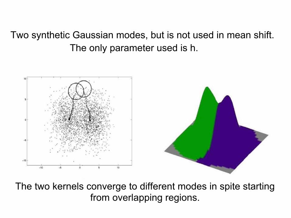
Two synthetic Gaussian modes, but is not used in mean shift. The only parameter used is h.

The two kernels converge to different modes in spite starting from overlapping regions.

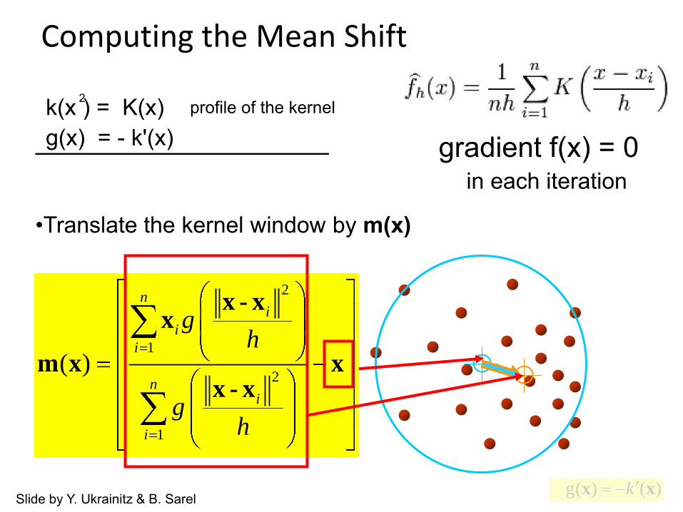
•Translate the kernel window by m(x)

2

1

2

1

( )

ni

i

i

ni

i

gh

gh

x - xx

m x xx - x

g( ) ( )kx x

Computing the Mean Shift

Slide by Y. Ukrainitz & B. Sarel

k(x ) = K(x)g(x) = - k'(x)

2 profile of the kernel

gradient f(x) = 0 in each iteration

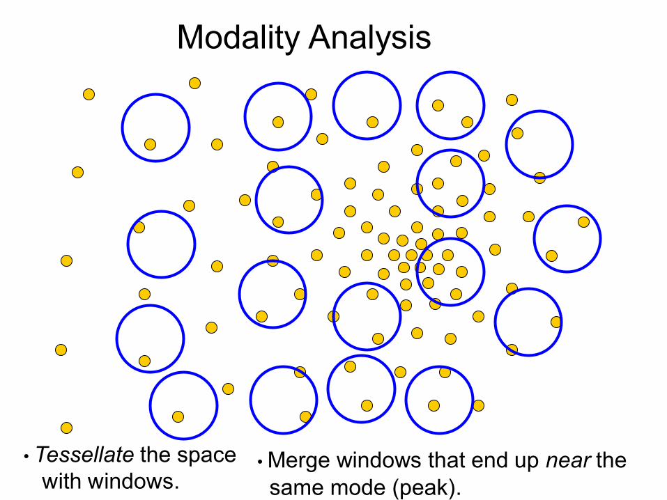
Modality Analysis

• Tessellate the space with windows.

• Merge windows that end up near the same mode (peak).

• !ǘǘNJŀŎǘƛƻƴ ōŀǎƛƴ: the region for which all trajectories lead to the same mode

• /ƭdzǎǘŜNJΥ all data points in the attraction basin of a mode

Slide by Y. Ukrainitz & B. Sarel

Attraction basin

Example: attraction basins

zero gradient, g(x)=0 but not a maximum stationary point eliminated by shifting a little bit the trajectory

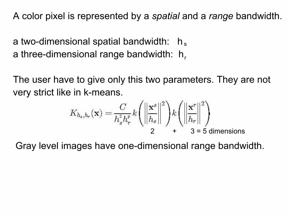
A color pixel is represented by a spatial and a range bandwidth. a two-dimensional spatial bandwidth: ha three-dimensional range bandwidth: h The user have to give only this two parameters. They are notvery strict like in k-means.

2 + 3 = 5 dimensions

Gray level images have one-dimensional range bandwidth.

s

r

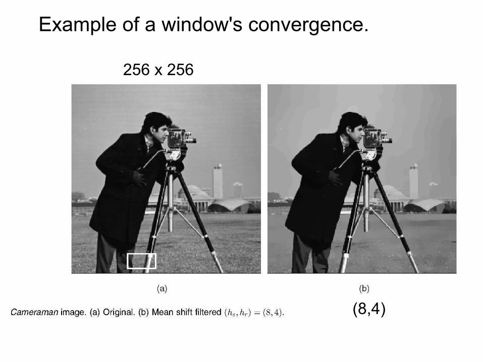
Example of a window's convergence.

256 x 256

(8,4)

original(inverted)

mean shift

filtering segmentation

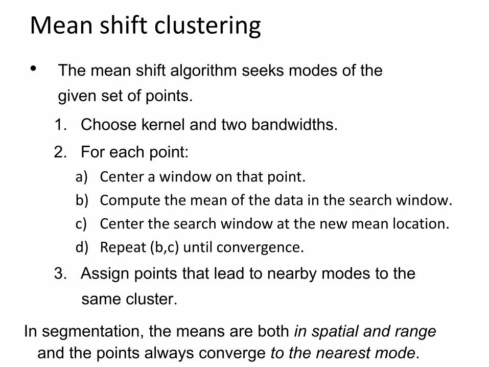
Mean shift clustering

• The mean shift algorithm seeks modes of the given set of points.

1. Choose kernel and two bandwidths.

2. For each point: a) Center a window on that point.

b) Compute the mean of the data in the search window.

c) Center the search window at the new mean location.

d) Repeat (b,c) until convergence.

3. Assign points that lead to nearby modes to the same cluster.

In segmentation, the means are both in spatial and range and the points always converge to the nearest mode.

Mean shift clustering are two phases: filtering, as was described before; segmentation, unify adjacent clusters if they are closer than h_s in the spatial domain and h_r in the range domain. (Step 3.) EDISON program can do additional things too, but we will not describe them here. Mean shift was also used for tracking of motions and fornonlinear spaces through Riemannian manifolds.

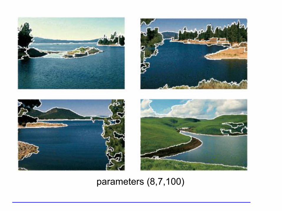
Mean shift segmentation results

Eliminate spatial regions containing less than M pixels.

512 x512

(16,7,40)

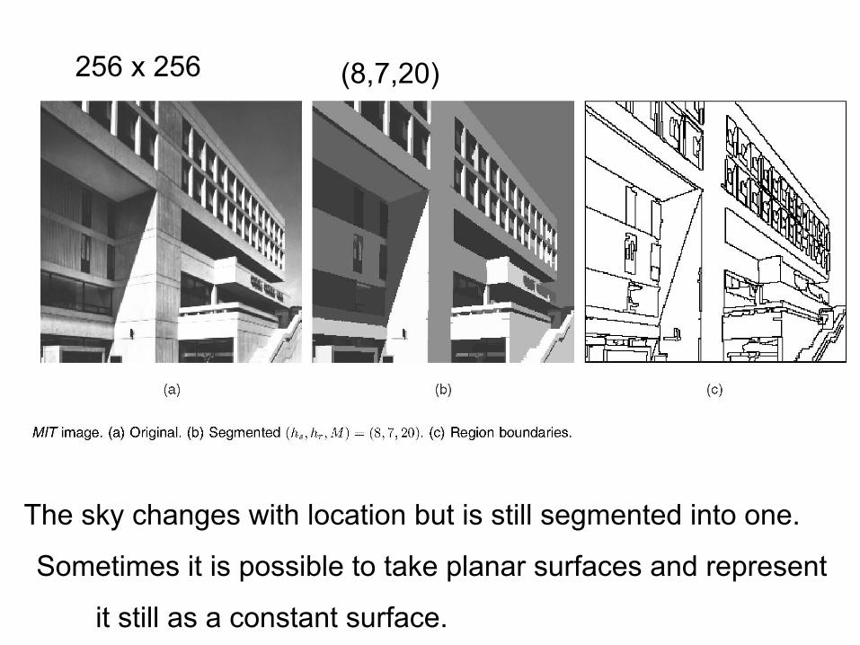
256 x 256

The sky changes with location but is still segmented into one.

Sometimes it is possible to take planar surfaces and represent

it still as a constant surface.

(8,7,20)

parameters (8,7,20)

parameters (8,7,100)

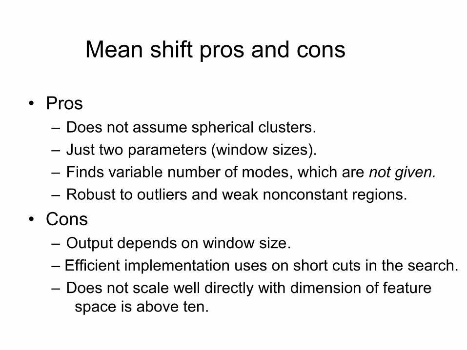
Mean shift pros and cons

• Pros – Does not assume spherical clusters. – Just two parameters (window sizes). – Finds variable number of modes, which are not given. – Robust to outliers and weak nonconstant regions.

• Cons – Output depends on window size. – Efficient implementation uses on short cuts in the search. – Does not scale well directly with dimension of feature

space is above ten.

Berkeley Segmentation Engine

http://www.eecs.berkeley.edu/Research/Projects/CS/vision/grouping/

one of the best segmentation groups

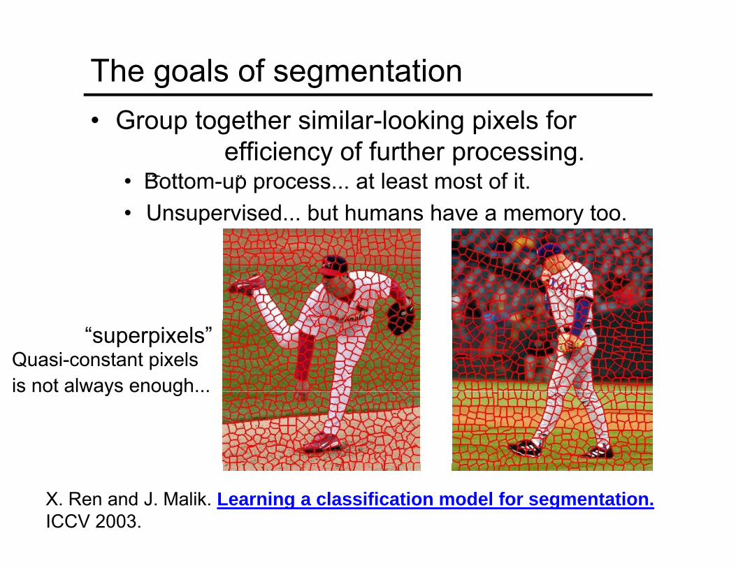
The goals of segmentation• Group together similar-looking pixels for

efficiency of further processing.“B tt ”• Bottom-up process... at least most of it.

• Unsupervised... but humans have a memory too.

“superpixels”

X. Ren and J. Malik. Learning a classification model for segmentation.ICCV 2003.

Quasi-constant pixelsis not always enough...

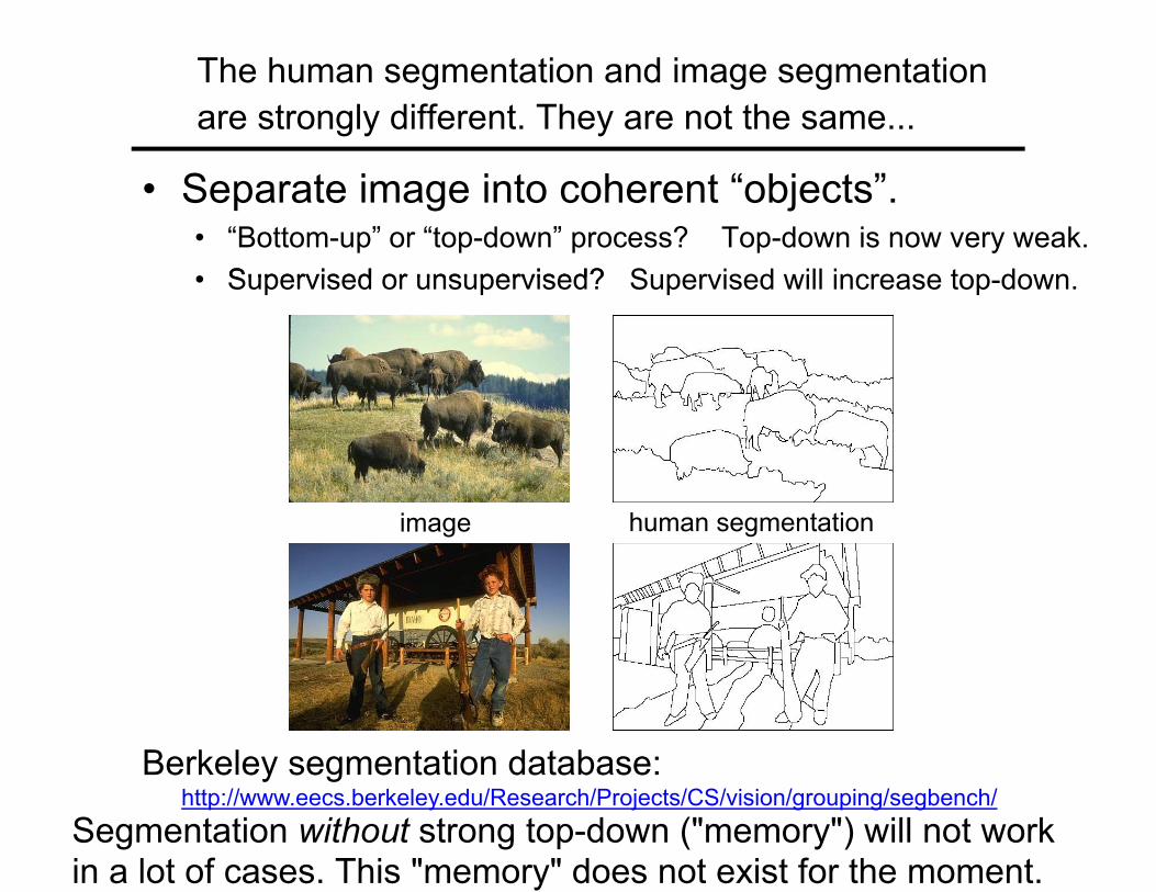
• Separate image into coherent “objects”.• “Bottom-up” or “top-down” process? Top-down is now very weak.• Supervised or unsupervised?• Supervised or unsupervised? Supervised will increase top-down.

image human segmentation

Berkeley segmentation database:http://www.eecs.berkeley.edu/Research/Projects/CS/vision/grouping/segbench/

Segmentation without strong top-down ("memory") will not workin a lot of cases. This "memory" does not exist for the moment.

The human segmentation and image segmentationare strongly different. They are not the same...

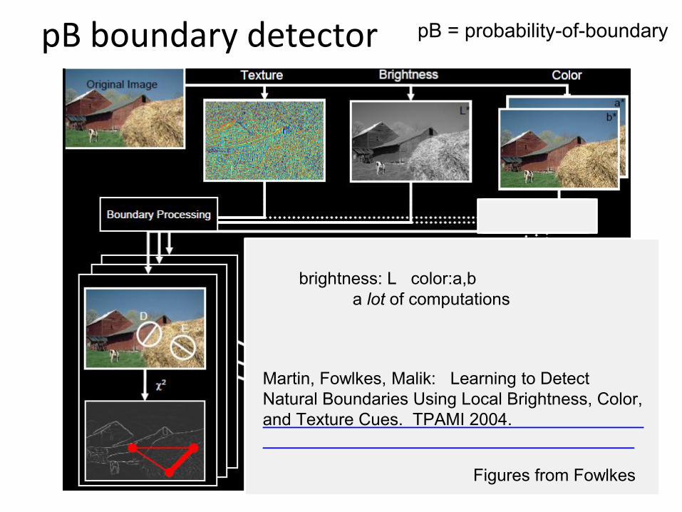
pB boundary detector

Figures from Fowlkes

Martin, Fowlkes, Malik: Learning to Detect Natural Boundaries Using Local Brightness, Color,and Texture Cues. TPAMI 2004.

pB = probability-of-boundary

brightness: L color:a,ba lot of computations

pB Boundary Detector

intensity

brightness

color

texture

Brightness

Color

Texture

Combined

Human

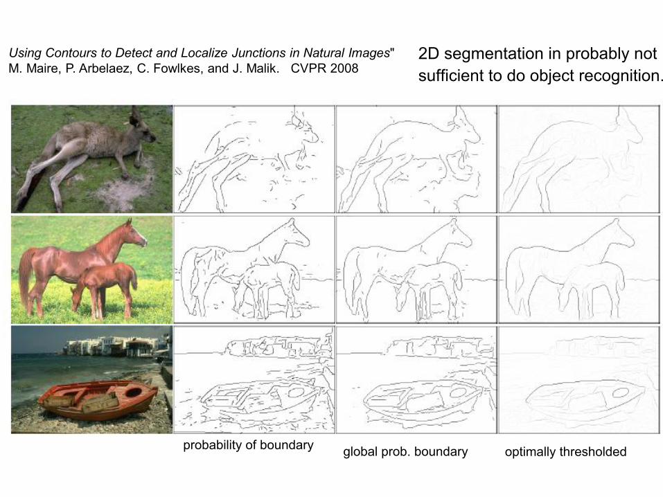
Using Contours to Detect and Localize Junctions in Natural Images" M. Maire, P. Arbelaez, C. Fowlkes, and J. Malik. CVPR 2008

probability of boundary

optimally thresholdedglobal prob. boundary

2D segmentation in probably notsufficient to do object recognition.

45 years of boundary detection

Source: Arbelaez, Maire, Fowlkes, and Malik. TPAMI 2011 (pdf)

TS/(TS+FS)

TS/(TS+FG)True/FalseSegm./Ground

human ground-truth boundaries

(correct +unexpected)

(correct + missing)

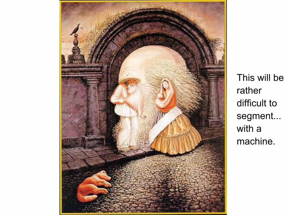
This will berather difficult tosegment...with amachine.