CMBS and Conflicts of Interest: Evidence fromOwnership Changes for Servicers∗

Maisy Wong†University of Pennsylvania

October 2016

Abstract

Self-dealing is potentially important but difficult to measure. I study special servicers in com-mercial mortgage-backed securities (CMBS), who sell distressed assets on behalf of bondhold-ers. Around 2010, ownership changes for four major servicers raised tunneling concerns thatthey may direct benefits to new owners’ affiliates (buyers and service providers). Loans liq-uidated after ownership changes have greater loss rates than before (8 percentage point, $2.3billion in losses), relative to other (placebo) servicers. Together with a case study that tracksself-dealing purchases, the findings point to potential steering conflicts that could incentivizetunneling through fees to service providers.

∗I am grateful to Fernando Ferreira, Joe Gyourko, and Todd Sinai for their advice. I thank Santosh Anagol, EffiBenmelech, Serdar Dinc, Mark Garmaise, Kristopher Gerardi, Laurie Goodman, Jean-Francois Houde, Pamela Lee,Christopher Palmer, Sergey Tsyplakov, Nikolai Roussanov, seminar participants at Penn State University, Universityof Virginia, Wharton, and conference participants at the AREUEA-ASSA annual conference, Housing-Urban-Labor-Macro (HULM), NBER Summer Institute, WFA Summer Real Estate Research Symposium, and the University ofSouthern California Research Symposium. Rachel Brill, Ying Chen, Hye Jin Lee, Jeremy Kirk, Will Lin, LauraNugent, Joon Yup Park, Rebecca Pierson, Xuequan Peng, Dean Udom, Xin Wan, and Justine Wang were excellentresearch assistants. I am also grateful to market participants who shared their experiences with me in confidence. Ithank the Research Sponsors Program of the Zell/Lurie Real Estate Center at Wharton, the Jacobs Levy Grant, andthe Wharton Dean’s Research Fund for research support. All errors are my own.†Wharton Real Estate. 3620 Locust Walk, 1464 SHDH, Philadelphia, PA 19104-6302. Email:

maisy@wharton.upenn.edu.

1 Introduction

Self-dealing has been alleged to harm investors but it is hard to measure (Shleifer and Vishny,1997). The wave of foreclosures of securitized assets has put a spotlight on intermediaries thatmanage securitized assets on behalf of bondholders. There is anecdotal evidence that some inter-mediaries appear to tunnel private benefits to their affiliates at the expense of distant bondholders(Lee, 2014). However, it is hard to quantify the extent of self-dealing for securitized assets becauseit is hard to track them after securitization. Moreover, self-dealing incentives are endogenous bynature and often correlated with omitted variables.

The commercial mortgage-backed securities (CMBS) market provides a useful context to ad-dress the empirical challenges in the self-dealing literature. It is the second most important sourceof credit in the commercial real estate sector with total assets of $623 billion (Federal Reserve,2016). Each CMBS trust comprises a pool of mortgages that are collateralized by non-residentialproperties. Crucially, it is relatively easier to track the chain of ownership of CMBS assets becausereal estate transactions are recorded publicly.

I study self-dealing concerns involving four of the major special servicers in the CMBS market,servicing around $500 billion of CMBS debt in 2010. Special servicers are debt firms managingdistressed mortgages on behalf of bondholders with the goal of maximizing the net present value ofassets. When a loan is non-performing, the special servicer decides whether and how to liquidateit. Loan liquidations typically involve selling the collateral (non-residential properties). As sellers,special servicers have to search for buyers and intermediaries to facilitate the liquidation.

Around 2010, ownership changes for the four special servicers linked them with new affili-ates, presenting potential self-dealing conflicts. The new owners are vertically integrated financialinstitutions with affiliates that may be potential buyers of CMBS liquidations or potential inter-mediaries that facilitate real estate transactions (lenders, brokers, and online auction platforms).The scales of the servicers can present efficiency benefits and complementarities for the verticallyintegrated business models of the new owners, helping to overcome significant search frictions incommercial real estate. However, the links to the new affiliates also heightened concerns that spe-cial servicers may be incentivized to sell assets at a discount to the new owners or to steer businessopportunities to affiliates to earn fees.

At the same time, the volume of distressed CMBS assets, which remained relatively low before2010, started to increase sharply. Market participants grew concerned that these two factors (the

1

rise in potential sales by servicers and the potential links to affiliates) would sharply increase thepotential for these servicers to self-deal with affiliates. Yoon (2012) reports that special servicersappear to be “burdened by conflicts of interest caused in part by new ownership” and allegedly“cutting bad deals”.

Motivated by concerns over the ownership changes for the four servicers, I begin by estimat-ing the impact of these events on outcomes for liquidated loans. I compare the changes in loanloss rates (realized losses divided by loan balance before losses) for the four (treated) special ser-vicers before and after their ownership changes relative to other (placebo) servicers. The placeboservicers have fewer affiliates with potential tunneling conflicts, relative to the treated servicers.

I find that loans liquidated after treated special servicers changed owners have loss rates that are8 percentage points higher than before, relative to placebo servicers. This translates into aggregatelosses of $2.3 billion, representing 20% of total losses from liquidations by treated servicers undernew ownership.

My panel data analysis includes 9272 loans liquidated from 2003 to 2012, controls for spe-cial servicer fixed effects, month of liquidation fixed effects, and pre-determined loan attributes.The key regressor is the interaction between an indicator for loans liquidated by treated servicersand an indicator for liquidations after ownership changes. The identification assumption is thatunobserved determinants of loan loss rates do not change differentially for treated versus placeboservicers, conditional on the fixed effects and loan attributes.

I present robustness checks to address several threats to identification. Since the events hap-pened around 2010, a key confounder is unobserved market conditions. Here, the placebo ser-vicers serve as counterfactuals to the extent treated and placebo servicers face common marketconditions. The effect remains stable using various controls for market conditions. Second, whileloans are not randomly assigned across servicers, trends in the quality of liquidated loans indicatethat compositional differences in loans are unlikely to explain away the main effect.

Another major threat relates to the liquidity crises that triggered the ownership changes fortreated servicers. Like many debt firms, when credit spreads widened from 2008 to 2009, thebalance sheets worsened dramatically for the previous owners of the servicers, triggering the needfor capital infusion. Treated servicers could have been relatively more capacity constrained andoverwhelmed by their own problems, accumulating a stockpile of distressed debt. The concern isthat some of the differences in losses after the ownership changes reflect differences in stockpilingbefore the ownership changes. Moreover, the stockpiling effect is merely a transitory difference

2

that dissipates once the stockpile of debt has been resolved (even while new ownership remained).To address concerns that the greater loss rates for treated servicers are confounded by a (tran-

sitory) stockpiling effect, I show that the results survive excluding the 18 months right before andafter the ownership changes. Additionally, the patterns remain similar if I exclude a three-yearwindow instead of 18 months, using auxiliary data from Bloomberg which provides a longer postperiod (6 years instead of 3 years). This suggests the results are not driven by transitory con-founders.

Next, I provide a bounding exercise to assess how much of the difference in losses in the postperiod could be driven by the stockpiling effect instead of the ownership change effect. Uncondi-tional trends in the volume of losses reveal a bunching pattern, with an “excess mass” in lossesafter ownership changes that may reflect new owners’ liquidations of the stockpile of distresseddebt. However, a conservative bounding exercise shows that stockpiling explains at most 21% ofthe difference in losses.

Importantly, there are no bunching patterns for conditional trends, perhaps because both treatedand placebo servicers did not anticipate the sudden increase in distressed debt. Indeed, conditionaldifferences between treated and placebo servicers reveal no bunching pattern, after controlling forservicer and month fixed effects. Overall, while self-dealing concerns generally arise in endoge-nous settings, the weight of the evidence suggests the 8 p.p. greater loss rate is unlikely to beexplained away by the confounders discussed above.

Turning to mechanisms, I explore the three self-dealing conflicts raised by market participants:(i) buying (new owners buying assets sold by special servicers), (ii) steering (servicers steeringbusiness opportunities to affiliated service providers and earning fees), and (iii) price discrimina-

tion (affiliated service providers charging bondholders higher fees to sell CMBS assets). The pricediscrimination channel suggests bondholders would pay greater liquidation expenses. However, Ifind that liquidation expenses are not higher after ownership changes for treated servicers, relativeto placebo servicers, which is inconsistent with the price discrimination channel.

Next, I estimate that liquidations after ownership changes have an average sale price that is14% lower than before, relative to placebo servicers. The magnitude of this price discount is largeenough to explain the $2.3 billion in aggregate losses reported above. Notably, monthly liquidationvolumes increase by 229% for treated servicers relative to placebo servicers. The price discountand increase in liquidation volume are consistent with both the buying and steering channels.

To assess the relative importance of the two channels, I complement the core regression analysis

3

with a case study for one treated servicer. I construct a novel dataset that tracks buyers for a sub-sample of 1000 CMBS properties liquidated by this servicer. Most real estate transactions arerecorded publicly but the recorded owners are often limited liability companies. Since commercialproperties are high value assets, data firms have invested resources to collect information about thetrue owners. I hand-match a sub-sample of CMBS liquidations to property transactions to trackwhat happens to securitized assets liquidated by this servicer.

Strikingly, in contrast to the primary market concern over purchases, I only find 14 transactionspurchased by affiliates of the special servicer. However, a significant share of sales by this servicerinvolves affiliated service providers. These affiliated transactions are a central source of commis-sion revenue, constituting half of the total transaction volume for the affiliated brokers. I provide aback of the envelop calculation to illustrate the potential gains from fee streams that are consistentwith the magnitudes from the regression analysis above.

The limited purchases and relative importance of affiliated service providers point to the po-tential significance of the steering channel. This parallels concerns that relate the underpricingof IPO’s to commission generation by investment banks (Reuter, 2006; Nimalendran, Ritter, andZhang, 2007). The steering channel can be important in real estate, where many intermediaries areneeded to facilitate transactions. Each CMBS liquidation may represent a bundle of fee streamsfor affiliated service providers. By contrast, the purchasing channel may present greater litigationrisks (some servicers are being sued over self-dealing purchases).

These results shed light on the classic tension between the efficiency benefits from vertical inte-gration and the costs due to self-dealing conflicts in financial institutions. On balance, I find sizablelosses to CMBS bondholders that are consistent with concerns over tunneling conflicts but mixedevidence on scale efficiencies. I discuss three ways vertical integration can improve outcomes forbondholders, but do not find strong evidence of efficiency benefits. Bond-level analysis suggeststhe additional losses are concentrated amongst junior bonds but senior bondholders associated withtreated servicers do not have lower loss rates relative to placebo servicers.

One caveat is the imperfect coverage for affiliated service providers makes it harder to assessthe full extent of these affiliations. This is a common problem in the self-dealing context as it tendsto happen in places where self-dealing is hard to measure. I discuss on-going efforts to improvetransparency and provide some lessons for disclosure policies. Another caveat is that there may beother efficiency benefits that I do not observe.

This paper contributes to the literature on self-dealing and tunneling (Shleifer and Vishny,

4

1997). One approach assesses the extent of tunneling indirectly by investigating the relationshipbetween aggregate outcomes and self-dealing potential.1 Another approach uses transactions-leveldata to provide direct evidence of self-dealing in international contexts.2

My analyses build upon both approaches to make progress on the endogeneity and measure-ment challenges in the self-dealing literature. Motivated by market concerns, my core analysisconceptualizes ownership changes for the treated servicers as “shocks to firm affiliations” to pro-vide quasi-experimental variation in self-dealing potential. I study self-dealing in securitized debtmarkets in the United States and examine effects on both aggregate losses to bondholders as well asdisaggregated losses at the loan level. This allows me to investigate the three types of self-dealingmechanisms and control for potential confounders at a finer level. Moreover, the case study pro-vides the first transactions-level measure of self-dealing for securitized assets in the United States.

These findings in CMBS have important implications for the RMBS market as well. There isrelatively less work on agency conflicts after securitization (Keys et al., 2013), especially studieson what happens to assets that exit the MBS trust.3 Regulators have raised concerns over similarownership changes for RMBS servicers, especially non-bank servicers which have grown in im-portance and are relatively less regulated (FHFA, 2014). In fact, self-dealing conflicts involvingRMBS servicers and their affiliates are part of on-going investigations and lawsuits alleging ser-vicers directed businesses to benefit affiliates (Goodman, 2010; Lee, 2014).4 My analysis shedslight on potential self-dealing conflicts in the CMBS context, which can affect trust in securitized

1Bae, Kang, and Kim (2002) shows that the effects of acquisitions by Korean business groups on stock prices canhurt minority shareholders but controlling shareholders benefit through their affiliates. Lemmon and Lins (2003)compares the stock returns for firms with ownership structures that have varying degrees of self-dealing potentialduring the East Asian crisis. Djankov et al. (2008) studies the relationship between legal protection of minority rightsand stock market outcomes for 72 countries.

2Previous studies include analyses for markets in China (Jiang, Lee, and Yue, 2010), Hong Kong (Cheung, Rau, andStouraitis, 2006), Korea (Baek, Kang, and Lee, 2006), and Bulgaria (Atanasov, 2005). Kroszner and Strahan (2001),La Porta, de Silanes, and Zamarripa (2003), and Engelberg, Gao, and Parsons (2012) examine lending behavior forconnected lenders but focus on non-securitized debt.

3Agarwal et al. (2011) and Piskorski, Seru, and Vig (2010) study the effects of securitization on how RMBS servicersresolve distressed residential mortgages by comparing securitized loans against bank-held loans. Agarwal et al.(2015) and Maturana (2014) study the incentives of servicers to workout distressed residential mortgages. Withinthe CMBS literature, An, Deng, and Gabriel (2009) and Ghent and Valkanov (2015) investigate whether securitizedloans are adversely selected, Stanton and Wallace (2012) studies CMBS subordination levels and ratings. Gan andMayer (2006), Titman and Tsyplakov (2010), Ashcraft, Gooriah, and Kermani (2015), and Ambrose, Sanders, andYavas (2015) study other aspects of agency problems in CMBS.

4For example, the Superintendent of the New York Department of Financial Services raised "the possibility that man-agement has the opportunity and incentive to make decisions ... that are intended to benefit ... affiliated companies,resulting in harm to borrowers, mortgage investors..." (Lee, 2014)

5

markets and curtail investment activity (Zingales, 2015).The rest of the paper proceeds as follows. Section 2 describes the CMBS context, Section 3

describes the data, Section 4 presents the core analysis of the effect of ownership changes for thefour treated servicers. Section 5 discusses self-dealing and alternative considerations. Section 6concludes.

2 Background

2.1 Special servicers and ownership changes

A CMBS trust comprises a pool of mortgages collateralized by income-producing commercialproperties, such as apartments, hotels, warehouses, and retail properties. Each CMBS trust hasa master servicer which services loans that are current or expected to be recoverable. Loans thatare delinquent beyond applicable grace periods (typically 60 days) are transferred to the special

servicer, which usually takes over the operation of the commercial property from the borrower.5

It then decides whether to keep the distressed mortgage in the trust (by modifying the terms of themortgage) or not (usually by liquidating the asset).6

The servicing standard specified in pooling and servicing agreements generally requires specialservicers to maximize the net present value of assets on behalf of CMBS bondholders. However,special servicers have relatively wide latitude to use their judgement. They are appointed by thecontrolling class holder (usually the most junior tranche in the CMBS trust, known as the B-piece).B-piece buyers often appoint themselves as special servicers.7 Special servicers usually earn 25basis points on loans in special servicing, 1% of the resolved loan balance for loan resolutions(modifications or liquidations), and other fees, as stated in the pooling and servicing agreement.

Most special servicers are part of commercial real estate debt firms, with expertise in underwrit-ing commercial real estate debt and operating commercial properties. Like many debt investors,they faced liquidity crises when their balance sheets worsened because spreads widened in late2008. While the high yield debt investments suffered, their special servicing businesses grew5In contrast to residential MBS, in the event that borrowers default on their debt, special servicers are needed in CMBSfor their expertise in operating commercial properties.

6Technically, the special servicer can decide to sell the mortgage (a note sale) or to foreclose the property. In bothinstances, the loan will exit the CMBS trust.

7See Gan and Mayer (2006) and Ashcraft, Gooriah, and Kermani (2015) for studies related to this issue. I return tothis at the end of the paper.

6

in importance in light of the rise in delinquent loans after the crisis. Loans in special servicingincreased from $5 billion dollars in 2007 (0.5% of CMBS loans) to $90 billion dollars in 2012(12%).

I study the ownership changes for Berkadia (December 2009), C-III (March 2010), LNR (July2010), and CW Capital (September 2010). The four treated servicers are major special servicersin CMBS. Their scales present complementarities for the new owners’ vertically integrated busi-nesses. Using in-house intermediaries can speed up the liquidation process and having a largenetwork of customers can also facilitate the search and matching of buyers, lenders, and sell-ers. This can benefit bondholders (by improving liquidation outcomes) and also the new owners(through potential fee streams, and by building relationship capital or developing future businessopportunities).

Relative to the treatment group, the placebo servicers have fewer affiliates involved with CMBSliquidations. There are 30 placebo servicers with Midland being the largest and other moderately-sized servicers. Table A7 in the appendix lists the affiliates for each of the treated servicers and thetop 10 placebo servicers. These servicers are responsible for more than 80% of the liquidations inmy primary estimation sample.

Market concerns focused on the ownership changes for the four servicers. Table A7 shows thatthey are more likely to have affiliated brokerages, online auction platforms, and potential buyers.Some placebo servicers do not engage in acquisitions (several are part of banks that do not haveproprietary investments) and some emphasize that they do not use affiliated service providers tofacilitate CMBS liquidations. All servicers are lenders, but most placebo servicers are establishedlenders whilst some treated servicers are new lenders. The appendix (Section B) provides moredetails.

Figure 1 shows annual liquidation volumes remained below $2 billion through 2009 but startedto increase after that. Before the ownership changes, there was not much debt in distress. Therise in potential sales, combined with the potential links to new affiliates, contributed to a sharpincrease in concerns over potential self-dealing conflicts. Insofar as the placebo servicers or theprevious owners (in the pre-period) have the potential to engage in self-dealing as well, this wouldoperate against finding an effect.

These ownership changes were controversial and raised concerns among market participants.For example, Standard and Poor issued a statement that “combined with several ownership changespertaining to some of the largest commercial mortgage servicers, the rise in special servicing ac-

7

tivity has drawn increased market focus on potential conflicts of interests” (Steward et al., 2012).8

Steward et al. (2012) goes on to highlight a few self-dealing mechanisms, stating that “market par-ticipants...have expressed concern over special servicers’ exercising “fair market value” purchaseoptions, their use of affiliates, and the practice of charging additional fees in connection with loanrestructurings.”

2.2 Three types of self-dealing mechanisms

The concerns amongst market participants center around three types of self-dealing/tunnelingmechanisms that can arise in CMBS liquidations: (i) buying, (ii) steering, and (iii) price dis-crimination. Self-dealing/tunneling involves transactions that connect the special servicer (actingas a seller on behalf of bondholders) and any affiliate of the new owner, including a buyer or anaffiliated service provider.

First, when the ownership changes happened, the primary concern of the market was the abilityof special servicers to purchase a liquidated asset by exercising a fair value option. This optionallows the special servicer to purchase distressed assets in the CMBS trust at a fair value, as speci-fied in the pooling and servicing agreement. The ownership changes heightened the concerns overself-dealing via purchases because the new owners also had distressed debt investment funds andwere active buyers of commercial real estate assets. For example, a shareholder of Vornado (anew owner of LNR) stated that “I believe their goal here is to get first shot - potentially with nocompetitors - to buy mortgages which are being serviced by LNR ... Flow and exclusive first crackis the appeal.” (Troianovski and Wei, 2010)

The second mechanism, steering, relates to the concern that special servicers may be incen-tivized to steer business opportunities to affiliated service providers. For example, LNR had apartial ownership of an online auction platform (Auction.com) and there were concerns that LNRmay be incentivized to direct business opportunities to Auction.com by liquidating more assets.Similarly, other treated servicers also have affiliated lenders, brokerages, or titling agencies thatprovide various services to facilitate real estate transactions.

The third mechanism, price discrimination, is related to the possibility that affiliated serviceproviders might charge distant bondholders higher fees for their services when selling CMBSassets. For example, an RMBS servicer used an affiliated online auction platform (Hubzu) to8See also Berger (2012), Lancaster et al. (2012), and Wheeler (2012) for related commentary on potential agencyconflicts.

8

auction off foreclosed homes. Hubzu allegedly charged these affiliated auctions a fee of 4.5%(paid by bondholders) but charged fees as low as 1.5% for non-affiliated auctions it competes forin the open market (Lee, 2014).

3 Data

3.1 CMBS loans

I purchased access to CMBS loans data from November 2010 through November 2012 from Re-alpoint. This dataset includes the universe of all securitized loans. I observe loan attributes at-origination (such as loan-to-value (LTV), year of securitization, and the securitized loan amount)and information about the collateral (such as the property type, age, and the street address of theproperty). The appendix provides more details (Section A.1).

Crucially, the Realpoint database includes a realized loss report that comprises a history ofall securitized loans with realized losses to the CMBS trust, reporting the date the losses wereincurred, the loss rate, liquidation proceeds, liquidation expenses, as well as the balance beforelosses. There are 11,332 loans with realized losses, between September 1997 and November 2012.The primary estimation sample uses 9272 loans liquidated between 2003 and 2012. Before 2003,there are fewer than 500 liquidations per year.9

One shortcoming of this dataset is the lack of pre-treatment data for time-varying attributes.Realpoint only reports the most recent value for time-varying loan attributes (such as current LTV,current balance, and delinquency). Since all four ownership changes occurred before November2010, I do not have pre-treatment data for time-varying attributes. Table 1 reports the summarystatistics for the full sample of 120,495 securitized loans and the 9,272 liquidated loans in theprimary estimation sample.

I also use an auxiliary dataset from Bloomberg, with around 12,000 loans liquidated betweenJanuary 2000 and August 2016. The benefit of the Bloomberg dataset is the longer post period (6years instead of 3 years). However, Bloomberg only reports losses (the numerator for loss rates).I maintain the Realpoint data as the primary dataset as it is more comprehensive and I am able to

9My main specification includes special servicer fixed effects and month of liquidation fixed effects. Having moreliquidations in a year is useful because liquidation outcomes are noisy and in the earlier years, there is not muchvariation left after controlling for special servicer and month of liquidation fixed effects.

9

include more loan-level controls. Wherever appropriate, I use the Bloomberg data to show longertrends in the post period.

3.2 Measuring self-dealing relationships

As discussed in Section 2.2, market participants are most concerned about purchases by the newowners of special servicers. They are also concerned about the use of affiliated service providers.The core regression analysis uses comprehensive CMBS data covering loans liquidated by allservicers. This subsection describes measures of self-dealing relationships for one treated servicerin my case study.

I restrict my analysis to liquidations by C-III (which changed owners in March 2010). I choosethis special servicer because regressions by special servicer indicate that the patterns are mostrobust for this special servicer. The sample for the case study includes 1,074 properties that wereliquidated from 2010 to 2012 by C-III.

Purchases

To trace the chain of ownership, I handmatch data on CMBS loan liquidations with propertytransactions data. I use two databases of property transactions, CoStar and Real Capital Analytics.Both databases include information such as the transaction price, transaction date, address, as wellas the identity of the buyer. These databases focus on transactions above $2.5 million but alsoreport some CMBS transactions below this cutoff when available.

I limit the case study to one treated servicer only since the process of merging CMBS loanswith commercial property transactions is time consuming. Each property address for the 1,074properties had to be entered individually into these databases to search for the true owner for eachasset.10

Most transactions are structured so that buyers are limited liability companies (LLC). However,data firms have invested resources to collect information about the true identity of buyers, theiraddresses, and contact information. Commercial properties are high value assets and investors arewilling to pay for information about the true property owners for prospective investment or leasing

10While I only directly measure relationships for one servicer, the number of transactions is comparable to other papersin the literature. Baek, Kang, and Lee (2006) studies 262 private placements of equity-linked securities in Koreabetween 1989 and 2000. Cheung, Rau, and Stouraitis (2006) investigates pricing for connected transactions in 375filings in Hong Kong between 1998 to 2000. Jiang, Lee, and Yue (2010) examines 1,134 firm-years in their datawith information on affiliated transactions.

10

opportunities. Data vendors make significant attempts to identify the true owner, by contactingbrokers, property operators, and other sources. The exact methods are proprietary. Each recordis confirmed through multiple independent reports from reliable sources. For example, the buyerfor an apartment complex, Cherry Grove, is recorded publicly as RFI Cherry Grove LLC. But,the address for RFI Cherry Grove LLC is written in the deed as “RFI Cherry Grove LLC, c/oC-III Acquisitions LLC, 717 Fifth Avenue in New York”. Another commonly used address byC-III affiliates is 5221 North O’Connor Blvd, Suite 600, Irving, Texas. For transactions that wereidentified as being bought by C-III, I also obtained deeds of sales to confirm that the buyer isaffiliated with C-III.

Affiliated service providers

In addition to information about buyers, Real Capital Analytics also reports the brokers andlenders for property transactions, whenever this information is available. Compared to the data onbuyers, the coverage for service providers is less consistent, especially for lenders (sellers’ brokersare an important source of information for Real Capital Analytics). I searched for all transactionsfrom 2010 to 2015 that use an affiliate of C-III as the lender or the broker. The data coverage tendsto be more comprehensive for later years.

4 Effect of ownership changes for treated servicers

4.1 Effect on loan loss rates

Section 2 describes market concerns that losses increased after the ownership changes of the treatedservicers. I use a panel data specification that compares the changes in loan loss rates for treatedspecial servicers after they changed owners, relative to changes in loan loss rates for other (placebo)special servicers. Specifically, I estimate

LossRatelit = α +βOwnershipChangei×Postit + γXli + τt +δi + εlit (1)

where LossRatelit is the loss rate (realized losses divided by loan balance before losses) for loanl liquidated by special servicer i in month t (centered around event dates), OwnershipChangei is1 if servicer i is Berkadia, C-III, CW Capital, or LNR, and Postit is 1 if loan l is liquidated afterthe event date for special servicer i. For treated servicers, the event date corresponds to the first

11

day of the month they changed owners. For placebo servicers, Postit is 1 if month t is after LNR’sevent date. The results are similar using other placebo dates (Table 3). Additionally, Xli representspre-determined controls for loan l, τt is month of liquidation fixed effects, δi is special servicerfixed effects, and εlit is an idiosyncratic error term.

The parameter of interest is β which tests whether loss rates change differentially after treatedservicers changed owners compared to placebo servicers. The identification assumption is thatunobserved determinants of LossRatelit do not change differentially around the event dates fortreated versus placebo servicers, conditional on the controls. Standard errors are double clusteredby special servicer and month of liquidation.

Column 1 of Table 2 presents the main specification which indicates that loss rates for loansliquidated after treated servicers changed owners are 8 percentage points (p.p.) higher than before,relative to placebo servicers. This is a sizable effect, representing 16% of the mean loss rate (50%).This 8 p.p. effect translates into aggregate losses of $2.3 billion, representing 20% of total lossesby treated servicers under new ownership.11

The main specification includes controls that mitigate three sources of omitted variable bias.First, the ownership changes happened around 2010, raising the threat that the differences afterownership changes reflect sharp changes in economic conditions only. To the extent that assetsliquidated by placebo servicers face similar economic conditions, they can serve as useful coun-terfactuals. The trends for placebo servicers indicate lower and insignificant loss rates after 2010compared to before, as prices started to recover after 2010 (dashed line in Figure 1).

Additionally, the month of liquidation fixed effects control non-parametrically for high fre-quency monthly changes. Moreover, Table A1 in the appendix shows that the effects are similar(10 p.p. instead of 8 p.p.) with coarser time controls (quarter of liquidation, year of liquidationfixed effects, as well as monthly quadratic time trends plus a post indicator). The relative stabil-ity of the estimates mitigates concerns about confounding due to time trends (Altonji, Elder, andTaber, 2005).

Second, treated and placebo special servicers may not be comparable. I control special servicerfixed effects. Notably, before the ownership changes, the loss rates were lower for treated servicersrelative to placebo servicers.

Third, loans serviced by treated versus placebo servicers could be different. I control for pre-

11To calculate the total losses implied by the 8 p.p. effect on loss rates, I multiply it by the total balance before lossesfor all loans liquidated by treated servicers after the ownership changes ($29 billion).

12

determined loan attributes reported in Table 1, including the initial debt service coverage ratio(DSCR) and initial loan-to-value (two loan quality measures commonly used to underwrite com-mercial mortgages),12 initial loan balance, indicators for loans with balloon payments, with fixedinterest rates, indicators for property types (hotels, industrial properties, apartments, offices, re-tail), year of securitization, the number of properties, property age, and an indicator for loans withmissing loan attributes.

Columns 2 to 4 address concerns that β could be biased by other changes over time. Col-umn 2 adds interactions between loan attributes and the post indicator, to allow for the effectsof loan attributes on loss rates to be different before and after the ownership changes. Column3 adds MSA-by-year fixed effects to control for differences in local market conditions. Notably,the R-squared increases from 0.15 to 0.38, but the coefficient remains stable at 8 p.p.. Column 4adds special servicer-specific quadratic time trends and a post indicator (but drops month fixed ef-fects).13 This alleviates the concern that the loan quality is worsening over time differently acrossspecial servicers. Again, the effect is similar (9 p.p.).

Table A2 in the appendix presents heterogeneous analyses using different sub-samples,demonstrating that the higher loss rates are not driven by particular loan types. The results aresimilar for fixed rate loans, office, and retail loans. Notably, the results are not significantly higherfor balloon loans (an indicator for high risk loans).

Robustness analysis

Table 3 further probes the robustness of the results on loss rates. The first row repeats themain specification in Table 2 (column 1) but includes liquidations in all years (1997 to 2012)instead of liquidations between 2003 and 2012. The next row includes liquidations between 2004and 2012. Row 3 repeats the main specification, restricting the sample to loans matched usingpropensity scores.14 Row 4 aggregates the loan level data to the special servicer-month level toaddress concerns of over-rejection (Bertrand, Duflo, and Mullainathan, 2004; Donald and Lang,

12The debt service coverage ratio is the net operating income of a property divided by the debt payment. Ratios above1 correspond to (safer) loans that have enough operating income to cover debt payments. The initial loan-to-value isthe securitized loan amount divided by the value of the property.

13For placebo special servicers, I estimate a separate trend for Midland and a common trend for the other placeboservicers.

14I first predict the probability of treatment using a logit model with the treatment indicator as the dependent variable,loan controls and month of liquidation fixed effects. I then drop the 25% of loans in the control group with the lowestpredicted probability of treatment.

13

2007; Cameron, Gelbach, and Miller, 2008). The specification is analogous to that of the mainloan-level estimation. I include month fixed effects, special servicer fixed effects and report robuststandard errors in the parentheses.15 The next three rows repeat the main specification but use theevent dates for Berkadia, C-III, and CW Capital as placebo dates respectively. Row 8 repeats themain specification but further winsorizes loss rates at the top 1% to show that the results are notdriven by outliers. Reassuringly, the results are broadly similar across the specifications.

4.2 Differences in loan quality

This sub-section discusses potential concerns that the higher loss rates after the ownership changesof the treated servicers may be driven by compositional differences in loans. I consider differentmeasures of loan quality, including pre-determined loan attributes, time-varying attributes, as wellas trends in outcomes. I also provide a bounding exercise to assess the potential importance ofselection on unobservables.

4.2.1 Pre-determined loan attributes

Panel A of Table 4 tests for differences in pre-determined attributes for loans serviced by treatedversus placebo servicers. The first row reports results from an OLS regression with an indicatorfor fixed rate loans as the dependent variable and the ownership change indicator as the regressor.The sample comprises all loans that were securitized before 2008. Standard errors are clusteredby special servicer and month of securitization. Additionally, Figure A-1 to Figure A-5 in theappendix plot trends in these loan attributes for liquidated loans, to assess whether changes inthese cross-sectional differences can explain the higher loss rates in the post period.

While the loan composition is different along several dimensions, the trends cannot explain the8 p.p. higher loss rate. For example, loans serviced by the treatment group have an average initialLTV that is significantly higher by 3 p.p. (compared to a mean of 67%) but the trend is declining.This is inconsistent with higher initial LTV driving the higher loss rates. On average, DSCR islower by 0.02 and insignificant (compared to a mean of 1.49)

Another potential concern is that treated servicers are 41% more likely to have loans withballoon payments (relative to a mean of 74%), which could indicate worse loan performance.

15For the placebo servicers, I estimate a fixed effect for Midland and a common fixed effect for the other placeboservicers.

14

However, the results are robust to controlling for the balloon loan indicator and heterogeneousanalysis in Table A2 in the appendix shows that the results are not significantly stronger for balloonloans (column 2). Importantly, the trend for the balloon indicator (second panel in Figure A-1) isdecreasing, which indicates that fewer balloon loans are liquidated over time.

Table 4 also shows that loans serviced by treated special servicers have larger loan balances,are more likely to have fixed interest rates, more likely to be a hotel, office, or retail loan, and arenewer. However, their trends are relatively stable and mitigate the concern that the higher loss ratesare driven by a decline in the quality of liquidated loans for treated servicers.

In addition, Table A3 in the appendix tests for location differences by including indicators forhousing bust markets as the dependent variable. Reassuringly, treated loans are not significantlymore exposed to housing bust markets.

4.2.2 Time-varying attributes

Turning to time-varying attributes, ideally, it would be nice to compare these attributes before andafter ownership changes to see if loan quality worsened differentially more for treated servicers.I do not have pre-2010 data for time-varying attributes (Section 3). Below, I first discuss treatedversus placebo differences in current LTV and current DSCR. Then, I discuss trends in the 60-daydelinquency rate.

Panel B of Table 4 reports the average differences in current LTV and current DSCR for thesample of current loans. Figure 2 plots the trends.16 For current LTV, the average is 4.6% higherfor treated loans (p-value of 5%), but the trend is relatively stable (the maximum change in LTV is1 p.p.). For current DSCR, the average difference is -0.002 and insignificant. The trend is decliningslightly over time. As a benchmark, the maximum decline of -0.04 translates into an increase inloss rates of 0.4 p.p. only.17

Turning to liquidated loans, Panel C of Table 4 indicates that current LTV is higher by 1.6 p.p.but the difference is not significant and current DSCR is significantly higher (safer) by 0.1. The

16For Table 4, I regress current LTV for loan l, serviced by servicer i, reported in month t, on a treatment indicatorand on report month fixed effects (centered around the event dates). The sample includes 893,906 loan-monthobservations, comprising all loans with positive current balances in month t. Standard errors are double clustered byservicer and report month. For Figure 2, I add interactions between the treatment indicator and month fixed effects.I do not have enough months to estimate double clustered standard errors for the figure. The conclusions are similarwith robust standard errors, clustering by servicer, or no clustering. I chose the most conservative of the three.

17The correlation between loss rates and current DSCR is -0.1.

15

trends in Figure 3 do not indicate any sharp changes for liquidated loans right after time 0. Thisis not consistent with treated servicers resolving a stockpile of distressed debt right after the newowners relaxed their capacity constraints.

Next, I examine differences in the 60-day delinquency rate. This represents a relatively exoge-nous measure of loan quality as special servicers have less control over these loans because mostloans are only transferred to special servicers after they become delinquent for more than 60 days.

On average, treated loans are 0.2% more likely to become 60-day delinquent, relative to amean of 0.3% and a standard deviation of 1% (column 1 of Table A4 in the appendix).18 Figure 4demonstrates that the trends appear stable. The higher 60-day delinquency rate for treated servicersis a potential concern, though it would have been ideal to test if this difference is greater relativeto the pre-period.

Importantly, loan-level analysis demonstrates that the 60-day delinquency is unlikely to bethe main driver of the higher loan loss rates (columns 2 to 5 in Table A4). Conditional on pre-determined loan controls, treated loans are not more likely to become 60-day delinquent in mysample period. The difference (0.005) is insignificant and small relative to the mean (0.06). Theresults are similar weighting observations by their current balance (column 3). Moreover, loans thatbecome 60-day delinquent in my sample do not have higher loss rates (column 4). Finally, aug-menting my main specification with a triple interaction (post dummy, ownership change dummy,and a dummy for delinquent loans) delivers an insignificant coefficient (column 5), indicating thatthe 8 p.p. effect on loss rate is not driven by these delinquent loans only. I provide more details inthe appendix.

In summary, while the servicer-month level analysis indicates treated servicers are more likelyto have loans that become 60-day delinquent, the loan-level analysis suggests this difference isunlikely to explain the higher loan loss rates I find above.

4.2.3 Trends in outcomes

The top panel of Figure A-6 presents annual estimates of β for the loss rate analysis (equation 1).Relative to year -6 (the omitted group), differences in loss rates in the pre-period are negative fortwo years and positive for three years. While the average effect (8 p.p.) is significant in my mainspecification, the confidence intervals are wide for the annual estimates.

18The dependent variable is the share of servicer i’s loans (in dollars) in month t that first become 60-day delinquentin month t and the controls include month fixed effects.

16

The bottom panel of Figure A-6 presents conditional trends in the monthly volume of losses,using the longer post period from Bloomberg. Bloomberg only reports losses (the numerator forloss rates). I estimate equation (2) below.

lnLossit = βOwnershipChangei×Postit + τt +δi + εit (2)

where the dependent variable, lnLossit measures the monthly volume of losses (Lossit = ∑l Losslit

aggregates over losses from loan l liquidated by servicer i in month t). In the pre-period, theestimates are positive for 1 year and negative for 4 years. In the post period, the coefficientsare consistently positive, with an average effect of 0.84, significant at the 1% level (column 1 ofTable A6).

Finally, as an overall assessment of the potential importance of omitted variable bias, I followAltonji, Elder, and Taber (2005) and Oster (2016) to calculate how large selection on unobserv-ables will need to be to explain away the entire 8 p.p. effect on loan loss rates. My calculationssuggest selection on unobservables will have to be twice as important, which is twice as large asthe heuristic cutoff of one. Table A5 in the appendix provides more details.

Overall, the discussion above addresses concerns related to specific loan quality measures,including pre-determined loan attributes, time-varying loan attributes, locations, loss rates, andvolume of losses. While there are some differences and loans are not randomly assigned acrossservicers, the weight of the evidence suggests differences in loan quality cannot explain the 8 p.p.greater loss rate.

4.3 Stockpiling effect and liquidity crises before ownership changes

Next, I address the concern that the higher loan loss rates are driven by the liquidity crises thattriggered the ownership changes. The concern is treated servicers were capacity constrained beforethe ownership changes as they were too occupied with their own problems and built a stockpileof distressed loans that should have been liquidated. Therefore, the higher loss rates could reflecta transitory difference in the quality of liquidated loans that dissipates after treated servicers haveresolved the stockpile of distressed debt.

First, it is worth noting that the servicing operations of the treated servicers were relativelywell-functioning even while the high yield debt investments weakened the balance sheets for the

17

firms. In addition, both treated and placebo servicers did not anticipate the sudden spike in thevolume of distressed CMBS debt. For example, a rating agency report by Fitch in 2009 (justbefore the ownership changes) stated that “Fitch continues to believe current staffing levels areat capacity for most special servicers” (Petosa, Weems, and Carlson, 2010). To the extent thatplacebo servicers also experienced crisis-like moments, comparing differences between treatedand placebo servicers helps to address this issue.

Second, if treated servicers liquidate the worst loans first, this would result in a divergencein trend right after the ownership change, followed by a convergence towards placebo servicers.However, I do not observe such patterns, as discussed in Section 4.2. Next, I discuss additionaltests and a bounding exercise to further address concerns related to the stockpiling channel.

4.3.1 Dropping years right around ownership changes

Table 5 addresses the concern that the greater loss rate in the post period reflects transitory con-founders such as the stockpiling channel. Column 1 repeats the main specification with the fullestimation sample (8 p.p. effect). Column 2 reports a 10 p.p. effect after dropping a year beforeand after the ownership changes, column 3 reports a 13 p.p. effect after dropping 18 months. Asa benchmark, the average real estate owned (REO) hold time is 12 months for 2012 (Heschmeyer,2014).

Reassuringly, the effects remain robust across the three columns. These estimates are notstatistically different from each other. Table A6 in the appendix shows that the patterns are ro-bust to dropping up to 3 years before and after the ownership changes, using auxiliary data fromBloomberg.

Together, these additional tests suggest the greater losses are not due to confounders that aretransitory in nature. Otherwise, the effects would disappear after dropping the years right aroundthe ownership changes.

4.3.2 Bounding exercise for stockpiling effect

Next, I present a back of the envelop bounding exercise to assess the potential importance of thestockpiling channel. The top panel of Figure 5 presents unconditional trends in the monthly vol-ume of losses (Lossit) using servicer-month level data aggregated from Bloomberg. The two linescorrespond to trends estimated using local linear regressions, for the average treated servicer (top

18

line) and the average placebo servicer (bottom line). For the treated servicer, there is a bunchingpattern in the post period. This excess mass in losses after time 0 may stem from the stockpile ofdistressed debt accumulated before time 0. Placebo servicers also exhibit a similar trend (with aless pronounced pattern given the scale).

The concern is that the difference in losses may be driven by both an ownership change effect

plus a stockpiling effect. The stockpiling effect arises if a part of the difference in losses after

time 0 stems from a difference in stockpiling before time 0. I begin by assuming a counterfactualof no capacity constraints, to estimate how much more treated and placebo servicers could haveliquidated before time 0. Under this extreme case, the counterfactual trends would rise sharplywhen the crisis hit (like a step function).

The bottom panel of Figure 5 illustrates this. This figure is identical to the top panel, buthighlights three areas important for the bounding exercise. To the right, the difference in lossesbetween month 0 and month 36 (the post period in my estimation sample) amounts to $2.6 billion.The goal is to assess how much of the $2.6 billion can be explained by the stockpiling effect. Ibriefly describe the three main steps and provide more details in the appendix (Section A.2.9):

Step 1: First, I estimate the maximum increase in losses for treated servicers assuming no capacity con-

straints (Area T=$708 million). I repeat the same for placebo servicers (Area C=$168 million).

Step 2: The stockpiling effect is the additional difference in losses before time 0 (Area T − Area C =

$540 million). This represents the difference that could have happened before time 0, assuming the

servicers were not delayed by their capacity constraints.

Step 3: So, stockpiling explains at most 21% of the difference in losses ( $540million$2.6billion =0.21).

The appendix explains why 21% is likely a conservative upper bound. Importantly, Figure A-7 shows that there is no bunching pattern for conditional trends (differences relative to placeboservicers, controlling for servicer and month fixed effects). This is consistent with the notion thatboth treated and placebo servicers faced capacity constraints. Therefore, the regression analysislikely differences out part of the stockpiling effect and the bounding exercise using unconditionaldifferences is likely conservative.

In summary, while self-dealing is endogenous by nature and there is no random assignment ofself-dealing relationships, the weight of the evidence suggests that changes in market conditions,differences in loan quality, and the stockpiling of distressed debt are unlikely to explain away themain effect.

19

5 Is it self-dealing?

So far, the finding of higher loan loss rates after ownership changes is consistent with market con-cerns. As discussed in Section 2.2, there are three types of self-dealing mechanisms: (i) buying, (ii)steering, and (iii) price discrimination. While these channels may not be mutually exclusive, thissection presents a collection of findings that lend more support to the steering channel comparedto the buying and price discrimination channels.

5.1 Why are loan loss rates higher?

Loan losses can be greater either because assets are liquidated at lower prices or fees incurred tosell the assets are higher. Column 1 explores the sale price channel using a hedonic regression withlog sale price as the dependent variable, special servicer fixed effects, quadratic time trends (anda post indicator), MSA fixed effects, and pre-determined controls.19 Column 2 repeats the samespecification using log of liquidation expenses as the dependent variable.

Table 6 shows that the higher loss rates reflect lower sales prices for the liquidated assets.The estimate suggests the average price is 14% lower for assets liquidated by treated servicersafter ownership changes relative to placebo servicers. I calculate that the price discount needed torationalize the $2.3 billion in aggregate losses implied by the main effect (Table 2, column 1) isaround 10%, which is similar to the price discount estimated here.20

Column 2 shows there is no significant effect on liquidation expenses, which is inconsistentwith the price discrimination channel. If treated servicers are charging bondholders higher fees tosell the assets, this should lead to greater liquidation expenses after the ownership changes relativeto placebo servicers.

Interestingly, column 3 shows that treated servicers are liquidating more after ownershipchanges. The dependent variable measures the dollar volume of liquidation by special serviceri in month t using ln(∑l BalanceBe f oreLosslit), where I sum over the balance before losses for allloans liquidated by special servicer i in month t. This aggregates the data to the special servicer-month level and controls for month fixed effects and special servicer fixed effects. The estimate

19The sale price is missing for about a third of the sample. This sample attrition is not significantly different for treatedversus placebo servicers.

20The total sales proceeds from liquidations by treated servicers in the post period is $21 billion. Assuming thecounterfactual sales proceeds total $23.3 billion ($2.3 billion more), the price discount is 10% (2.3/23.3).

20

represents an increase in the liquidation volume by 119 log points (229%), or an increase of $105million per special servicer per month, using the pre-event average of $46 million.21

5.2 Case study: Self-dealing transactions for one servicer

So far, the regression estimates of higher loan loss rates, lower prices, and greater liquidation vol-ume are inconsistent with the price discrimination channel and consistent with both the buying andthe steering channels. The buying channel is naturally associated with lower prices (as affiliatedbuyers prefer lower prices) but it can also be associated with a greater liquidation volume if specialservicers are incentivized to liquidate and steer investment opportunities to affiliated buyers.

The steering channel is also consistent with an increase in liquidation volume and lower prices.For example, when a buyer approaches the special servicer to bid for a distressed asset, the servicercould inform the buyer privately that it would accept a lower price if the buyer uses its in-houseservice providers. This tunneling example directs private revenue streams to the servicer’s affiliatesto the detriment of bondholders (who suffer from the lower sale price).

This subsection presents evidence from a case study for one treated special servicer (C-III).In March 2010, Island Capital purchased Centerline (the predecessor of C-III) and the servicingrights for $110 billion of CMBS debt, with $100 million in equity and $180 million of assumeddebt. Andrew Farkas, Chairman and CEO of Island Capital, described a vertically integrated busi-ness strategy for this acquisition: “With C-III we are seeking to acquire real estate oriented debtderivatives and to build special servicing and ancillary businesses to manage those.” (Cohen, 2010)

Limited purchases

To track the chain of ownership to see whether C-III is selling assets to affiliates, I merge thesample of CMBS liquidations by C-III with property transactions data. I then identify whether thetrue buyer is an affiliate of C-III, as discussed in Section 3.2.

Contrary to market concerns about self-dealing through purchases, I only find 14 propertytransactions, valued at $171 million, that were bought by C-III. This could be due to the threatof litigation (some special servicers are involved in lawsuits pertaining to the use of the fair valueoption to purchase CMBS assets) and the high profile nature of this self-dealing conflict. For

21This increase in liquidation volume is not consistent with adverse selection concerns by unaffiliated buyers (theymay be willing to pay less for loans liquidated by treated servicers if they expect treated servicers to sell the bestloans to affiliates).

21

example, a few transactions (linking special servicers and the new owners) were presented as the“poster children of questionable behavior” (Yoon, 2012).22

Even though many investors thought the servicers would engage in self-dealing by buyingassets, these reports and the threat of litigation may increase the costs to engage in self-dealingthrough purchases. This is consistent with research on the importance of institutions that protectinvestors (Djankov et al., 2008).

Affiliated service providers

In contrast to the limited purchases identified above, affiliated service providers appear to beimportant. While the coverage for data on affiliated service providers is weaker than the coveragefor buyers, I provide several sources of information that point to the importance of these providers.

First, Chamberlain and Merriam (2015) reports that the share of Real Estate Owned (REO)sales using an affiliated broker was 30% in 2011 and 90% in 2014. Second, property transactionsdata from Real Capital Analytics suggests that C-III (the servicer) engages an affiliate in 40% oftransactions. Third, data from Real Capital Analytics indicate that close to half of the total trans-action volume of C-III’s affiliated brokers involve liquidations where C-III is the special servicer.In other words, liquidations from C-III’s servicing arm is a central source of commission revenuefor C-III’s affiliated brokers.

How much can the new owners potentially gain through tunneling?

To illustrate the potential importance of the steering channel, I provide a back of the envelopcalculation that shows that C-III can stand to gain up to 70% of the losses to bondholders. Of the$2.3 billion in losses for all 4 treated servicers implied by the regression estimates (Table 2), $462million is associated with C-III. During the post period, sales proceeds from CMBS liquidationsby C-III total $3.6 billion.

I consider the potential gains to C-III through the benefits to its affiliated lender, brokers, andtitling agency in facilitating the $3.6 billion in liquidations. The expected profits from lendingamount to $89 million.23 The potential gains from brokerage and titling services amount to $234

22Also, when a high profile property in New York (666 Fifth Avenue) was sold to Vornado (the new owner of LNR),this transaction received much media attention. As the lawyer representing the sellers explained, “Vornado got“anything but” an advantage from its stake in the special servicer...Everybody knew what was going on.” (Levitt,2011).

23To estimate this, I assume an LTV of 80% and a loan yield of 8% (based on the general lending parameters onC-III’s website). I further assume a 3% charge-off rate and a profit margin of 40%. I estimate the charge-off rate

22

million. This assumes a commission rate for brokerage services of 6% and 0.5% for titling.24

Together, the total potential gains are $323 million (70% of $462 million), multiplied by theshare of transactions that engage affiliated service providers. Assuming shares of 30% or 90%(using the lowest and highest estimates above) would imply that C-III can gain 21% to 63% ofthe $462 million losses to bondholders. These magnitudes are consistent with the larger lossesreported in the regression analysis. In addition, there could also be dynamic spillover benefits inthe form of future business opportunities. In this sense, the purchase of C-III can be viewed as aninvestment in relationship capital.

These potential gains in fee streams and the 14% price discount (Table 6) show how unaffiliatedbuyers and affiliated service providers can potentially benefit at the expense of bondholders. Sincecommissions and potential fee streams are usually relatively fixed and not a large percentage ofthe sale price, the marginal benefit from selling at a higher price is not large (Levitt and Syverson,2008). Many intermediaries tend to focus on transaction volume to drive revenue, and may offerprice discounts to unaffiliated buyers to attract them. This can be important for new businessestrying to develop relationships and gain market share. Moreover, bondholders do not have muchrecourse as the servicing standard in the typical pooling and servicing agreement gives specialservicers quite a bit of latitude on how they structure liquidations (unlike the fiduciary standard).

5.3 Potential benefits from vertical integration

Of course, vertical integration has potential efficiency benefits as well. I consider three benefitsbelow.

Higher liquidation price

The fair value option, which allows special servicers to bid for distressed assets, can lead tohigher sales prices, especially in situations where there are few or no bidders. Special servicers maybid higher prices for distressed assets relative to other investors if they have private informationabout the underlying quality of the asset. However, the price discount and greater loan loss ratesreported above are inconsistent with this benefit.

and the profit margin from recent annual reports of publicly traded mortgage REITs. I estimate the profit marginfrom reported average loan yields and reported average cost of funds or from the income statements. Put together,the expected profits are calculated as (1-0.03)*($3.6 billion*80%*8%*40%).

24I estimate these parameters from market reports and conversations with practitioners. I do not have data on profitmargins for these services.

23

Faster liquidations

Next, using in-house intermediaries can lead to faster liquidations. On average, liquidationsby treated servicers are 1.7 months faster relative to placebo servicers. This analysis relies on acomparison between treated and placebo servicers in the post period only as I do not have pre-period data for time to liquidation.25 Together, the 14% lower sale price reported in Table 6 andthe faster time to liquidation implies a monthly discount rate of 8%, suggesting the price discountsappear too steep.

While I do not have pre-period data, a back of the envelop calculation suggests liquidationshave to be 7 months faster (relative to the pre-period) to rationalize the 14% price discount.26

An improvement of 7 months is quite large, considering the average REO holdtime is 12 months(Heschmeyer, 2014). Also, rating agency reports do not indicate significantly faster liquidationsafter the ownership changes.27

B-piece conflict and benefits to senior bondholders

A third benefit of having vertically integrated affiliates pertains to benefits for senior bond-holders because the self-dealing conflicts have the potential to offset another conflict in the CMBSstructure which tends to hurt senior bondholders. In CMBS, the owner of the first loss tranche(B-piece) acts as the controlling class holder and often appoints itself as the special servicer. Thisconcentration of control rights in (thin) first loss tranches incentivizes special servicers againstliquidating loans to prevent the B-pieces from being wiped out. This protects their control rights,potentially at the expense of senior bondholders. In light of the B-piece conflict which reduces liq-uidation, the steering channel which incentivizes more liquidation, can have an off-setting effect.28

25The dependent variable is the number of months between 60-day delinquency and liquidation. I include loan con-trols, time trends, and MSA fixed effects. The sample comprises 2153 loans with data on time to liquidation. Thecoefficient on the ownership change indicator is significant at the 5% level and the standard error is 0.7.

26I use an annual discount rate of 25% (this is at the higher end of target returns for opportunistic real estate investmentfunds), which implies a monthly discount rate of 1.9%. Therefore, the improvement in speed has to be 7 monthsfaster (the ratio of 14% and 1.9%).

27Steward and Wertman (2013) report that the average time it took C-III to foreclose loans ranged from 8 to 11 monthsbefore the ownership changes (2008-2010) but it increased to 16 to 18 months after the ownership changes (2011 to2012). Chamberlain and Merriam (2015) also report that average resolution times were not consistently faster forsales using affiliated brokers relative to non-affiliated sales.

28The B-piece holder affects liquidation outcomes through the appointment of special servicers. Since I observe fewerthan 100 loans in my estimation sample with changes in special servicers, any potential bias is likely controlled forusing special servicer fixed effects (Section A.1).

24

My analysis of bond-level losses suggests that the additional losses are concentrated amongstjunior bonds but senior bond holders do not have lower loss rates for treated servicers compared toplacebo servicers. I downloaded bond-level loss rates (realized losses divided by original balance)from Bloomberg in April 2016. The average loss rate for bonds is 23%.

Treated bonds have an average loss rate of 26% compared to 18% for placebo bonds. Thelosses are concentrated amongst junior bonds (original rating below A). For senior bonds (originalrating of A or better), the loss rates are similar (3.7% for treated and 3.5% for placebo). Likewisefor AAA-rated bonds (0.3% for treated and 0.2% for placebo).

It is possible that absent the ownership changes, senior bondholders may suffer even greaterlosses. However, this bond-level analysis is suggestive that the self-dealing mechanism is notenough to lead to lower loss rates for senior bondholders. The appendix provides more detailsabout the bond-level data (Section A.1).

5.4 Discussion

Overall, the chain of evidence above is less consistent with the buying and price discrimina-tion channels, but point to the importance of potential steering conflicts. On balance, I findsizable losses to bondholders after the ownership changes, consistent with concerns over self-dealing/tunneling conflicts. However, I find mixed evidence of efficiency benefits.

Impact on trust and broader investment activity

While the self-dealing mechanisms discussed above can be viewed as transfers from bondhold-ers to the new owners and buyers of CMBS liquidations, there could also be broader efficiencylosses that can arise from reduced trust. Figure 6 plots the issuance volume (in billions of dol-lars) and market shares for special servicers, by year of issuance. Two striking patterns emerge.First, annual CMBS issuance volumes have dropped markedly after the crisis even while othercommercial debt instruments have grown in importance.

Second, treated servicers have lost market share. The market share for Midland has increased.Discussions with market participants suggest that Midland has the reputation of being a neutralspecial servicer because it has no proprietary investment activity. While these are suggestive pat-terns only, they are consistent with the interpretation that investors’ concerns with agency conflicts

25

amongst treated special servicers could endanger trust in the market and curtail investment activ-ity.29

Unmeasured connections and lessons for disclosure policies

In principle, more disclosure of affiliated transactions can improve transparency and enhancetrust in CMBS markets. The Investor Reporting Package (IRP) developed by the CommercialReal Estate Finance Council provides a standardized reporting template used widely by servicers,trustees, and data providers in CMBS. At present, there are templates to disclose the involvementof affiliates and the fees charged. However, this information is only provided at the discretion ofthe special servicer. Moreover, lending relationships are not tracked comprehensively.

To restore trust in the CMBS market, one proposal is to encourage the public disclosure of af-filiated transactions. In similar efforts, the Securities Exchange Commission (SEC) is encouragingthe disclosure of non arms’-length fees by private equity firms (SEC, 2015).

6 Conclusion

The ownership changes and new business models for four CMBS special servicers provide a lens tostudy the tension between the benefits of vertical integration and the costs of self-dealing conflicts.Compared to placebo servicers, treated servicers liquidate loans with higher loss rates, lower salesprices, and they also liquidate more after they changed owners. These findings are consistent withself-dealing concerns raised by market participants. I do not find many purchases by new ownersbut affiliated service providers are potentially important. There is mixed evidence on whetherthe use of affiliates speed up liquidation. I provide a battery of robustness checks and boundingexercises to show that selection is not likely to explain away the main effect.

These findings have broader implications. For example, the Dodd-Frank Act calls for the im-plementation of risk retention requirements in securitized markets. While the rule targets adverseselection before securitization, one unintended consequence is that it could enhance agency con-flicts after securitization. The high costs of the risk retention requirements could limit competitionfrom small issuers and servicers (Geithner, 2011). As the number of servicers in the securitiesmarket declines, the likelihood of self-dealing conflicts increases because the servicers that remain

29Recently, nine major issuers and bondholders issued a letter to raise concerns that current servicing practices weredamaging the industry’s reputation (Commercial Mortgage Alert, 2016).

26

are likely those with ties to major financial institutions, further exacerbating self-dealing concerns.This also lends support to the importance of independent intermediaries and third party monitors,emphasized in the Dodd-Frank Act.

In future work, it would be interesting to study other aspects of agency conflicts in securitizedmarkets and how they may interact with the risk retention policy and with potential tunnelingconflicts. Another direction for research is to investigate how the disclosure of information affectsoutcomes. Finally, how important are tunneling conflicts in the RMBS context? Servicers inthe residential sector also experienced ownership changes and non-bank servicers are growing inimportance.

27

ReferencesAgarwal, Sumit, Gene Amromin, Itzhak Ben-David, Souphala Chomsisengphet, and Douglas D. Evanoff.

2011. “The Role of Securitization in Mortgage Renegotiation.” Journal of Financial Economics 102:559–578.

Agarwal, Sumit, Gene Amromin, Itzhak Ben-David Souphala Chomsisenghpet, and Yan Zhang. 2015. “Sec-ond Liens and the Holdup Problem in Mortgage Renegotiation.” NBER Working Paper No.20015.

Altonji, Joseph, Todd Elder, and Christopher Taber. 2005. “Selection on Observed and Unobserved Vari-ables: Assessing the Effectiveness of Catholic Schools.” Journal of Political Economy 113 (1):151–184.

Ambrose, Brent W., Anthony B. Sanders, and Abdullah Yavas. 2015. “Servicers and Mortgage-BackedSecurities Default: Theory and Evidence.” Real Estate Economics 44 (2):462–489.

An, Xudong, Yongheng Deng, and Stuart A. Gabriel. 2009. “Asymmetric Information, Adverse Selection,and the Pricing of CMBS.” Journal of Financial Economics 100:304–325.

Ashcraft, Adam B., Kunal Gooriah, and Amir Kermani. 2015. “Does Skin-in-the-Game Affect SecurityPerformance? Evidence from the Conduit CMBS Market.” Working Paper, Federal Reserve Bank ofNew York.

Atanasov, Vladimir. 2005. “How Much Value can Blockholders Tunnel? Evidence from the Bulgarian MassPrivatization Auctions.” Journal of Financial Economics 76:191–234.

Bae, Kee-Hong, Jun-Koo Kang, and Jin-Mo Kim. 2002. “Tunneling or Value Added? Evidence fromMergers by Korean Business Groups.” The Journal of Finance 57 (6):2695–2740.

Baek, Jae-Seung, Jun-Koo Kang, and Inmoo Lee. 2006. “Business Groups and Tunneling: Evidence fromPrivate Securities Offerings by Korean Chaebols.” The Journal of Finance 61:2415–2449.

Berger, Stacey M. 2012. “The New World Order for Special Servicers: Is the Cure Worse Than the Dis-ease?” CRE Finance World 14 (2):15–18.

Bertrand, Marianne, Esther Duflo, and Sendhil Mullainathan. 2004. “How Much Should We TrustDifferences-in-Diferences Estimates?” Quarterly Journal of Economics 119:249–275.

Cameron, A Colin, Jonah B Gelbach, and Douglas L Miller. 2008. “Bootstrap-Based Improvements forInference with Clustered Errors.” The Review of Economics and Statistics 90 (3):414–427.

Chamberlain, Mary and Michael S. Merriam. 2015. “Operational Risk Assessments: C-III Asset Manage-ment, LLC.” Morningstar, June.

Cheung, Yan-Leung, P. Paghavendra Rau, and Aris Stouraitis. 2006. “Tunneling, Propping, and Expropri-ation: Evidence from Connected Party Transactions in Hong Kong.” Journal of Financial Economics82:343–386.

Cohen, Jeffery P. 2010. “Island Capital Group LLC Annouces Acquisition.” Business Wire, March 08.

Commercial Mortgage Alert. 2016. “Issuers, Investors Rebuke CMBS Servicers.”

Djankov, Simeon, Rafael La Porta, Florencio Lopez de Silanes, and Andrei Shleifer. 2008. “The Law andEconomics of Self-dealing.” Journal of Financial Economics 88 (3):430–465.

28

Donald, Stephen G. and Kevin Lang. 2007. “Inference With Difference-in-Differences and Other PanelData.” Review of Economics and Statistics 89 (2):221–233.

Engelberg, Joseph, Pengjie Gao, and Christopher A. Parsons. 2012. “Friends with Money.” Journal ofFinancial Ecnomics 103:169–188.

Federal Housing Finance Agency Office of Inspector General (FHFA). 2014. “FHFA Actions to ManageEnterprise Risks from Nonbank Servicers Specializing in Troubled Mortgages.” AUD-2014-014, July 1.

Federal Reserve Board (Federal Reserve). 2016. “Financial Accounts of the United States: Flow of Funds,Balance Sheets, and Intergrated Macroeconomic Accounts.” Federal Reserve Statistical Release, March10.

Gan, Yingjin Hila and Christopher Mayer. 2006. “Agency Conflicts, Asset Substitution, and Securitization.”NBER Working Paper No.12359.

Geithner, Timothy F. 2011. “Macroeconomic Effects of Risk Retention Requirements.” Completed pursuantto Section 946 of the Dodd-Frank Wall Street Reform and Consumer Protection Act.

Ghent, Andra and Rossen Valkanov. 2015. “Comparing Securitized and Balance Sheet Loans: Size Matters.”Management Science :1–20Articles in Advance.

Goodman, Laurie. 2010. “Comment on Risk Retention in Securitization.” Amherst Securities Group LP,June 1.

Heschmeyer, Mark. 2014. “Length of Time to Dispose of CMBS REO Properties Increasing.” CoStar GroupNews: National, June 9.

Jiang, Guohua, Charles M.C. Lee, and Heng Yue. 2010. “Tunneling through Intercorporate Loans: TheChina Experience.” Journal of Financial Economics 98:1–20.

Keys, Benjamin J., Tomasz Piskorski, Amit Seru, and Vikrant Vig. 2013. “Mortgage Financing in theHousing Boom and Bust.” In Housing and the Financial Crisis, edited by Edward L. Glaeser and ToddSinai. University of Chicago Press, 143–204.

Kroszner, Randall S. and Philip E. Strahan. 2001. “Bankers on Boards: Monitoring, Conflicts of Interest,and Lender Liability.” The Journal of Financial Economics 62:415–452.

La Porta, Rafael, Florencio Lopez de Silanes, and Guillermo Zamarripa. 2003. “Related Lending.” QuarterlyJournal of Economics 118 (1):231–268.

Lancaster, Brian P., David Brickman, Victor Calanog E.J. Burke, Nelson Hioe, Michael Moran, ThomasF. Nealon III, Steve Kraljic, Jack Taylor, and Doug Tiesi. 2012. “Roundtable: Outlook 2012.” CREFinance World 14 (1):6–22.

Lee, Pamela. 2014. “Nonbank Specialty Servicers: What’s the Big Deal?” Urban Institute, August 4.

Lemmon, Michael L. and Karl V. Lins. 2003. “Ownership Structure, Corporate Governance, and FirmValue: Evidence from the East Asian Financial Crisis.”

Levitt, David M. 2011. “Kushner Reworks Debt on NYC’s 666 Fifth Ave. with Vornado.” Bloomberg,December 16.

Levitt, Steven D. and Chad Syverson. 2008. “Market Distortions When Agents Are Better Informed: The

29

Value of Information in Real Estate Transactions.” The Review of Economics and Statistics 90 (4):599–611.

Maturana, Gonzalo. 2014. “When are Modifications of Securitized Loans Beneficial to Investors?” Workingpaper, University of Texas at Austin.

Nimalendran, M., Jay R. Ritter, and Donghang Zhang. 2007. “Do Today’s Trades Affect Tomorrow’s IPOAllocations?” Journal of Financial Economics 84 (1):87–109.

Oster, Emily. 2016. “Unobservable Selection and Coefficient Stability: Theory and Evidence.” The Journalof Business Economics and Statistics Forthcoming.

Petosa, Stephanie, Alyson Weems, and Richard Carlson. 2010. “CMBS YE 2009 Servicing Update: Reso-lution Trends, Special Servicing Loan Volume and Staffing Levels.” Fitch Ratings, March 15.

Piskorski, Tomasz, Amit Seru, and Vikrant Vig. 2010. “Securitization and Distressed Loan Renegotiation:Evidence from the Subprime Mortgage Crisis.” Journal of Financial Economics 97 (3):369–397.

Reuter, Jonathan. 2006. “Are IPO Allocations for Sale? Evidence from Mutual Funds.” The Journal ofFinance 61 (5):2289–2324.

Securities and Exchange Commission (SEC). 2015. “Blackstone Charged with Disclosure Failures.” Octo-ber 7.

Shleifer, Andrei and Robert W. Vishny. 1997. “A Survey of Corporate Governance.” The Journal of Finance52 (2):737–783.

Stanton, Richard and Nancy Wallace. 2012. “CMBS Subordination, Ratings Inflation, and Regulatory Cap-ital Arbitrage.” Working Paper, University of Berkeley.

Steward, Timothy, Mark Goldberg, Thomas Merck, Andrew Foster, Monica Perelmuter, Gary Carrington,and Barbara Hoeltz. 2012. “Standard & Poor’s Comments on Potential Conflicts of Interest WithinCommercial Special Servicing Market.” Global credit portal, Standard & Poor’s Financial Services.

Steward, Timothy E. and Pamela C. Wertman. 2013. “Servicer Evaluation: C-III Asset Management LLC.”Standard and Poor, September 20.

Titman, Sheridan and Sergey Tsyplakov. 2010. “Originator Performance, CMBS Structures, and the Riskof Commercial Mortgages.” Review of Financial Studies 23 (9):3558–3594.

Troianovski, Anton and Lingling Wei. 2010. “Vornado vs. Cerberus: LNR, Round2.” The Wall StreetJournal, June 9.

Wheeler, Darrell. 2012. “CMBS Special Servicer Behavior-As Subordinate Bond Positions Evolve FromInvestments to Fee Generators or Fair Market Value Options.” CRE Finance World 14 (1):29–34.

Yoon, Al. 2012. “Investors Bemoan Lean Results from Workouts.” The Wall Street Journal, May 29.

Zingales, Luigi. 2015. “Does Finance Benefit Society?” Prepared for the 2015 AFA Presidential Address.NBER Working Paper No. 20894.

30

Tables

Table 1: Summary statistics

All loans Liquidated loans

Variable name: N Mean SD N Mean SD1(Fixed rate loan) 120495 0.90 0.30 9272 0.87 0.34

1(Balloon loan) 120495 0.74 0.44 9272 0.69 0.46

1(Property is hotel) 120495 0.04 0.20 9272 0.06 0.24

1(Industrial property) 120495 0.07 0.25 9272 0.05 0.22

1(Property is apartment) 120495 0.28 0.45 9272 0.26 0.44

1(Retail property) 120495 0.24 0.43 9272 0.20 0.40

1(Property is office) 120495 0.13 0.34 9272 0.14 0.35

Year of securitization 120495 2002 3.56 9272 2003 3.50

Initial loan balance (in million dollars) 115896 7.78 15.31 8658 6.69 12.30

Number of properties per loan 120495 1.24 4.75 9272 1.21 3.83

Property age 87616 26.55 21.74 6571 26.33 20.23

Initial loan-to-value 110015 66.72 13.76 8543 70.97 9.75

Initial debt service coverage ratio 83636 1.49 0.54 6569 1.37 0.25

Loss rate 9272 0.50 0.49

Sale price (millions) 6375 5.94 12.49

Liquidation expense (thousands) 6307 797 1636

Notes: Summary statistics for pre-determined loan attributes for the full sample of 120,495 securitized loans (left 3columns) and the primary estimation sample of 9,272 liquidated loans (last 3 columns).

31

Table 2: Effect of ownership changes on loan loss rates

Main Post × MSA by ServicerSpecification: specification controls year FE trends

(1) (2) (3) (4)

Post × Ownership change 0.08*** 0.08*** 0.08*** 0.09**

( 0.03) ( 0.03) ( 0.02) ( 0.04)

N 9272 9272 9272 9272

R2 0.14 0.15 0.38 0.36

Month FE Y Y Y N

Special servicer FE Y Y Y Y

Controls Y Y Y Y

Post × Controls N Y Y Y

MSA-year FE N N Y Y

Special servicer time trends N N N Y

* p<0.1, ** p<0.05, *** p<0.01

Notes: This table reports results from OLS regressions using liquidated loans. The dependent variable is the loss rate forloan l liquidated by special servicer i in month t, centered around event dates. The loss rate is the loan losses divided bythe loan balance before losses. The key regressor is the interaction between an indicator that is 1 if special servicer i istreated and a post indicator that is 1 if month t is after the event date for special servicer i. The event date is the month ofownership change for treated servicers. The event date for placebo servicers is LNR’s event date. The estimation sampleconsists of 9,272 loans liquidated between 2003 and 2012. Column 1 reports the main specification with 106 month fixedeffects, 33 special servicer fixed effects and 13 pre-determined loan attributes (reported in Table 1), plus a dummy forloans with missing values for any loan attributes. Column 2 repeats column 1 but adds interactions between the postindicator and each loan control. Column 3 adds 1210 MSA-year fixed effects. Column 4 adds a post indicator, six specialservicer-specific quadratic time trends (and drops month fixed effects), including trends for each of the 4 treated servicers,Midland and a common trend for other placebo servicers. Standard errors are double clustered by special servicer andmonth of liquidation, with finite sample adjustments.

32

Table 3: Robustness checks for effect of ownership changes on loss rates

Coefficient Standard ErrorSpecification: (1) (2)

1. Sample: All years 0.10*** ( 0.03)

2. Sample: 2004-2012 0.06** ( 0.03)

3. Sample: Propensity score 0.09** ( 0.04)

4. Sample: Aggregated data 0.09** ( 0.04)

5. Placebo date: Berkadia date 0.10* ( 0.05)

6. Placebo date: C-III date 0.11** ( 0.05)

7. Placebo date: CW Capital date 0.06** ( 0.03)

8. Winsorize loss rates 0.08*** ( 0.03)

* p<0.1, ** p<0.05, *** p<0.01

Notes: The first row repeats the main specification in column 1 of Table 2 but includes all years (not just 2003-2012). Thesecond row includes a shorter event window (2004-2012). The third row repeats the main specification, restricting thesample to loans matched using propensity scores. The fourth row aggregates the loan level data to the special servicer-month level, 106 month fixed effects, 6 special servicer fixed effects (including a common fixed effect for placebo ser-vicers besides Midland), and robust standard errors. The next three rows repeat the main loan-level specification but usethe event dates for Berkadia, C-III, and CW Capital as placebo dates respectively. The last row winsorizes loan loss rateat the top 1 percent.

33

Table 4: Loan attributes for treated versus placebo servicers

Dependent variable: Mean SD N Coefficient Std. Err.

Panel A: All loans

1(Fixed rate loan) 0.90 0.30 120495 0.15*** ( 0.03)

1(Balloon loan) 0.74 0.44 120495 0.41*** ( 0.14)

Year of securitization 2002 3.56 120495 0.32 ( 0.72)

1(Property is hotel) 0.04 0.20 120495 0.03** ( 0.01)

1(Property is apartment) 0.28 0.45 120495 0.02 ( 0.04)

1(Retail property) 0.24 0.43 120495 0.15** ( 0.06)

1(Industrial property) 0.07 0.25 120495 0.01 ( 0.02)

1(Property is office) 0.13 0.34 120495 0.07** ( 0.03)

Initial loan balance (in million dollars) 7.78 15.31 115896 3.36** ( 1.58)

Number of properties per loan 1.24 4.75 120495 0.04 ( 0.10)

Property age 26.55 21.74 87616 -1.19** ( 0.54)

Initial loan-to-value 66.72 13.76 110015 3.17** ( 1.46)

Initial debt service coverage ratio 1.49 0.54 83636 -0.02 ( 0.02)

Panel B: Current loans

Current LTV 59.64 16.44 893906 4.62** ( 2.22)

Current DSCR 1.41 0.61 833718 -0.002 ( 0.03)

Panel C: Liquidated loans

Reported LTV at liquidation 65.23 11.81 4859 1.60 ( 1.99)

Reported DSCR at liquidation 0.93 0.56 4373 0.11** ( 0.05)

* p<0.1, ** p<0.05, *** p<0.01

Notes: Each row reports results from an OLS regression with a loan attribute as the dependent variable and the ownershipchange indicator as the key regressor. Panel A reports differences in pre-determined (at-origination) loan attributes. Thesample includes all loans securitized before 2008. Standard errors are double clustered by special servicer and month ofsecuritization. Panel B reports results for current loan-to-value ratios (LTV) for loan l in month t and current debt servicecoverage ratios (DSCR), controlling for report month fixed effects (centered by event dates) and clustering standard errorsby special servicer and report months. The sample includes all loans that have a positive loan balance in month t. Panel Ccompares the most recent LTV and DSCR reported for liquidated loans, controlling for month of liquidation and clusteringstandard errors by servicer and by liquidation month.

34

Table 5: Effect on loss rates (dropping years around ownership changes)

Dependent variable: Loan loss rate

Sample: Main Drop 1 Drop 18

spec year months

(1) (2) (3)

Post × Ownership change 0.08*** 0.10* 0.13**

( 0.03) ( 0.05) ( 0.06)

N 9272 5617 3937

R2 0.14 0.19 0.19

Month FE Y Y Y

Special servicer FE Y Y Y

Controls Y Y Y

* p<0.1, ** p<0.05, *** p<0.01

Notes: Column 1 repeats column 1 of Table 2. Column 2 drops one year before and after time 0. Column 3 drops 18months.

Table 6: Mechanisms related to higher loan loss rates

Dependent variable: Ln(Sale price) Ln(Expense) Ln(Volume)(1) (2) (3)

Post × Ownership change -0.14* -0.10 1.19***

( 0.08) ( 0.10) ( 0.14)

N 6375 6307 1132

R2 0.63 0.34 0.54

Month FE N N Y

Special servicer FE Y Y Y

Controls Y Y N

MSA FE Y Y N

Trends Y Y N

* p<0.1, ** p<0.05, *** p<0.01

Notes: Column 1 reports results from a hedonic regression where the dependent variable is log (Sale price) for theliquidated loan, the key regressor is the interaction between the ownership change and the post indicator, controlling forspecial servicer fixed effects, loan controls, MSA fixed effects, quadratic time trends (centered around event dates) and apost indicator. The sample includes liquidated loans in the estimation sample of Table 2 that have non-missing values forsales prices. Column 2 repeats the same regression with log of liquidation expenses as the dependent variable. Column3 aggregates the loan level data to the special servicer-month level. The dependent variable is log of the total amountliquidated by special servicer i in month t, where the total amount liquidated sums over the balance before losses for allloans liquidated by special servicer i in month t. This specification includes special servicer fixed effects, month fixedeffects and reports robust standard errors.

35

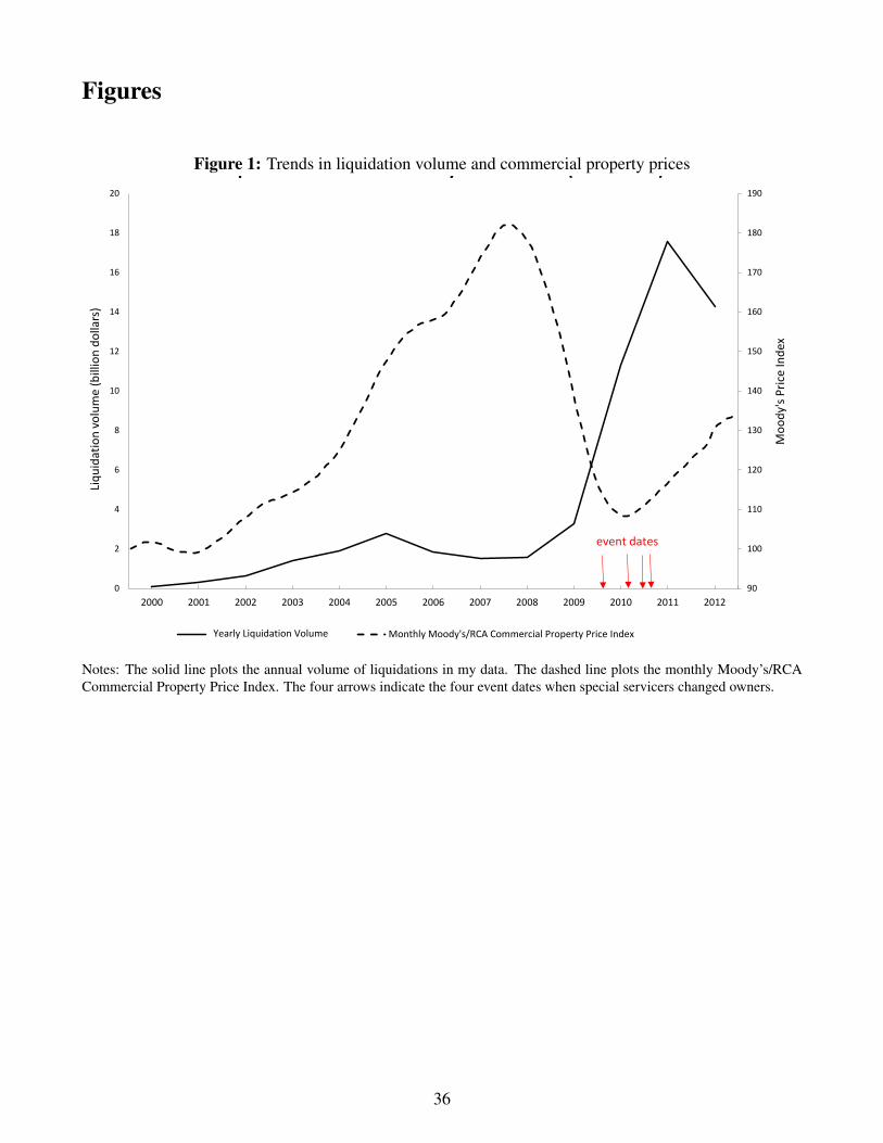
Figures

Figure 1: Trends in liquidation volume and commercial property prices

90

100

110

120

130

140

150

160

170

180

190

0

2

4

6

8

10

12

14

16

18

20

2000 2001 2002 2003 2004 2005 2006 2007 2008 2009 2010 2011 2012

Moo

dy's

Pric

e In

dex

Liqu

idat

ion

volu

me

(bill

ion

dolla

rs)

Liquidation Value and Moody's Price Index (2000-2012)

Monthly Moody's/RCA Commercial Property Price Index Yearly Liquidation Volume

Source: Moody's; Realpoint

event dates

Notes: The solid line plots the annual volume of liquidations in my data. The dashed line plots the monthly Moody’s/RCACommercial Property Price Index. The four arrows indicate the four event dates when special servicers changed owners.

36

Figure 2: Monthly trends for current debt service coverage and loan-to-value ratios

-.4

-.2

0.2

.4.6

.8C

urre

nt L

TV

12 13 14 15 16 17 18 19 20 21 22 23 24 25 26

-.06

-.05

-.04

-.03

-.02

-.01

0C

urre

nt D

SC

R

12 13 14 15 16 17 18 19 20 21 22 23 24 25 26

Notes: Each point reports monthly differences in current loan-to-value (LTV) and current debt service coverage ratio (DSCR),relative to month 11 (the omitted group), estimated from a regression of current loan attributes on a treatment dummy, reportmonth fixed effects and their interactions with the treatment dummy. DSCR equals net operating income divided by debt ser-vice payments. The sample includes all current loans, from November 2010 to November 2012. The ownership changes spanNovember 2009 (Berkadia) to September 2010 (CW Capital). The first relative month where I have current loan informationfor Berkadia is month 11. The figure ends at month 26 (the last relative month where I have current loan information for CWCapital). The dashed lines report 95% confidence intervals.

37

Figure 3: Monthly trends in debt service coverage ratio and loan-to-value for liquidated loans

-10

-50

510

15C

urre

nt L

TV

1 2 3 4 5 6 7 8 9 10 11 12 13 14 15 16 17 18 19 20 21 22 23 24 25 26

-.4-.2

0.2

.4.6

Cur

rent

DS

CR

1 2 3 4 5 6 7 8 9 10 11 12 13 14 15 16 17 18 19 20 21 22 23 24 25 26

Notes: Each point reports monthly differences in loan-to-value (LTV) and debt service coverage ratio (DSCR) reported forliquidated loans, relative to month 0, estimated from a regression of loan attributes on a treatment dummy, month of liquidationfixed effects and their interactions with the treatment dummy. The sample includes all loans liquidated in the post period, theomitted group is month 0. The dashed lines report 95% confidence intervals.

38

Figure 4: Monthly trend in share of loans that become 60-day delinquent

-0.010

-0.008

-0.006

-0.004

-0.002

0.000

0.002

0.004

0.006

0.008

0.010

Sha

re o

f loa

ns th

at b

ecom

e 60

-day

del

inqu

ent

13 14 15 16 17 18 19 20 21 22 23 24 25 26

Notes: Each point reports monthly differences in the share of loans (by dollar amount) that become 60-day delinquent inmonth t, estimated from a servicer-month level analysis with the treatment dummy, month fixed effects, and interactions withthe treatment dummy. Loans are transferred to special servicers after they become 60-day delinquent. The omitted group ismonth 12 (the first month where I have data to identify when a loan becomes 60-day delinquent). The dashed lines report 95%confidence intervals with robust standard errors.

39

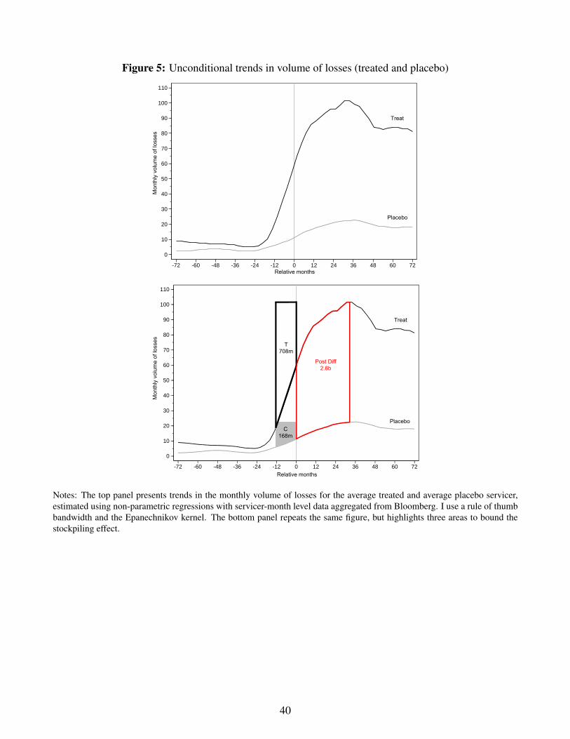
Figure 5: Unconditional trends in volume of losses (treated and placebo)

0

10

20

30

40

50

60

70

80

90

100

110

-72 -60 -48 -36 -24 -12 0 12 24 36 48 60 72

Treat

Placebo

Mon

thly

vol

ume

of lo

sses

Relative months

110

100

90

80

70

60

50

40

30

20

10

0

-72 -60 -48 -36 -24 -12 0 12 24 36 48 60 72

T708m

C168m

Relative months

Mon

thly

vol

ume

of lo

sses

Post Diff2.6b

Treat

Placebo

Notes: The top panel presents trends in the monthly volume of losses for the average treated and average placebo servicer,estimated using non-parametric regressions with servicer-month level data aggregated from Bloomberg. I use a rule of thumbbandwidth and the Epanechnikov kernel. The bottom panel repeats the same figure, but highlights three areas to bound thestockpiling effect.

40

Figure 6: CMBS issuance by year and market shares of special servicers

51%

62%

67%

11% 9%

21%

29%21%

49%38% 33%

89%

91%

79% 71%

79%

0

50

100

150

200

2005 2006 2007 2011 2012 2013 2014 2015

Issu

ance

vol

ume

(bill

ion

dolla

rs)

Figure 3: CMBS Issuance by Year and Market Shares of Special Servicers

Treated special servicers Placebo special servicers

TreatPlacebo

Notes: Each bar represents the total volume of CMBS debt issued each year between 2005 and 2007 and between 2011 and2015 for treated (darker bar) and placebo (lighter bar) special servicers, respectively. The annual issuance volumes between2008 and 2010 (ranging from $3 billion to $12 billion) have been suppressed. The numbers above the bars correspond to themarket shares for the treated and placebo special servicers.

41