cmpt 889: lecture 7 delay eﬀects: flanging, phasing ...tamaras/effects/effects.pdf · delay...

CMPT 889: Lecture 7Delay Effects: Flanging, Phasing, Chorus, Artificial

Reverb

Tamara Smyth, [email protected]

School of Computing Science,Simon Fraser University

October 26, 2007

1

mailto:[email protected]

http://www.cs.sfu.ca

http://www.sfu.ca

Flanging

• Flanging is a delay effect used in recording studiossince the 1960s.

• The effect was obtained by summing the outputs oftwo tape machines playing the same tape whiletouching the flange on one of the supply reals to slowit down, creating a delay between the two tapemachines.

• The flange is then released while touching the flangeon the other supply real, causing the delay togradually disappear and then grow in the oppositedirection.

flange

y(n)

Figure 1: Two tape machines are used to produce the flanging effect.

• We don’t hear echo because the delays are too short(typically 1-10 ms).

CMPT 889: Computational Modelling for Sound Synthesis: Lecture 7 2

Flanging Simulation

• Flanging creates a rapidly varying high-frequencysound by adding a signal to an image of itself that isdelayed by a short, variable amount of time.

• Since a delay between the two sources is needed, weshould expect that a delay line will be used in thedigital simulation.

• The delay however, must be a function of time (or thediscrete time variable n) so that it can be swepttypically from a few milliseconds (10ms or so) to 0 toproduce the characteristic flange sound.

• In the flange simulation, we use a feedforward combfilter given by the difference equation

y(n) = x(n) + gx[n − M(n)],

where the delay M(n) is variable over time.

gy(n)x(n) z−Mn

Figure 2: A simple flanger.


Delay parameter

• At any value of the delay M(n), the minima, ornotches, appear at frequencies that are odd

harmonics of the inverse of twice the delay time.

0 0.1 0.2 0.3 0.4 0.5 0.6 0.7 0.8 0.9 10

0.2

0.4

0.6

0.8

1

Comb impulse response with a delay of tau = 0.05

Time(s)

Am

plitu

de

0 10 20 30 40 50 60 70 80 90 1000

0.5

1

1.5

2

Comb amplitude response

Frequency (Hz)

Mag

nitu

de (

linea

r)

Figure 3: The impulse response and magnitude frequency response of a feedforward combfilter.

• Notches occur in the spectrum as a result ofdestructive interference (delaying a sine tone 180degrees and summing with the original will cause thesignal to disappear at the output).


The DEPTH parameter

• The feedforward coefficient g, also referred to as theDEPTH parameter, controls the proportion of thedelayed signal in the output, determining theprominence of the flanging effect.

• The DEPTH parameter sets the amount ofattenuation at the minima. It has a range from 0 to 1(where 1 corresponds to maximum attenuation).

0 10 20 30 40 50 60 70 80 90 1000

1

2

Comb Amplitude response for DEPTH 0.2

Frequency (Hz)

Mag

nitu

de (

linea

r)

0 10 20 30 40 50 60 70 80 90 1000

1

2


Frequency (Hz)

Mag

nitu

de (

linea

r)

0 10 20 30 40 50 60 70 80 90 1000

1

2


Frequency (Hz)

Mag

nitu

de (

linea

r)

Figure 4: Depth parameter controlling notch attenuation.

• It is possible to allow for dynamic flanging, where theamount of flanging is proportional to the peak of thesignal envelope passed through the flanger.


Variable Delay

• The characteristic sound of a flanger results whennotches sweep up and down the frequency axis overtime, dynamically altering the spectrum of the tonebeing processed.

• Since the delay is varying over time, the number ofdelay samples M must also vary over time.

• This is typically handled by modulating M(n) by alow-frequency oscillator (LFO). If the oscillator issinusoidal, M(n) varies according to

M(n) = M0[1 + A sin(2πfnT )],

where f is the rate of the flanger in cycles per second,A is the maximum delay swing, and M0 is the averagedelay length controlling the average notch density.

• If the flanging effect is properly, M must changesmoothly over time and therefore cannot have jumpsin values associate with rounding to the nearestinteger. We therefore must handle the fractionaldelay.


Interpolation and Fractional Delay

• To enable accurate tunings, and a smooth sweepingof M (particularly as the frequency approaches thesampling rate), it must be possible to create delaylines with fractional delay.

• Example interpolation techniques for achievingfractional delay:

1. Linear interpolation

2. Allpass interpolation

3. Lagrange interpolation


Linear Interpolation

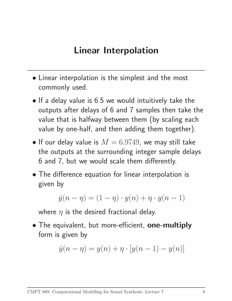
• Linear interpolation is the simplest and the mostcommonly used.

• If a delay value is 6.5 we would intuitively take theoutputs after delays of 6 and 7 samples then take thevalue that is halfway between them (by scaling eachvalue by one-half, and then adding them together).

• If our delay value is M = 6.9749, we may still takethe outputs at the surrounding integer sample delays6 and 7, but we would scale them differently.

• The difference equation for linear interpolation isgiven by

y(n − η) = (1 − η) · y(n) + η · y(n − 1)

where η is the desired fractional delay.

• The equivalent, but more-efficient, one-multiply

form is given by

y(n − η) = y(n) + η · [y(n − 1) − y(n)]


Allpass Interpolation

• Recall that an all-pass filter does not colour the soundby changing its frequency spectrum, but ratherchanges the phase of the signal by delaying it.

• The transfer function for the general first order allpassfilter is given by

H(z) =g + z−1

1 + gz−1

• Given the desired fractional delay δ, the feedback andfeedforward coefficient g is given by

g =1 − δ

1 + δ.

• Therefore, in a flange implementation where the delayis computed as fs/f0 = 17.87, a delay line would beset up with a sample delay of M = 17, followed by anallpass filter with the coefficient g calculated withδ = .87.

• Fractional delays are also useful to obtain moreaccurate tuning to a desired frequency.


Flanger vs. Phaser

• Flangers provide uniformly spaced notches. This canbe considered non-ideal given that this may cause adiscernible pitch to the effect.

• It can also cause a periodic tone to disappearcompletely through destructive interference. For thisreason, flangers are best used with inharmonic(non-periodic) sounds.

• A phaser (or phase shifter) is a close cousin of theflanger, and in fact, the terms are often usedinterchangeably.

• The noted difference is that phasers modulate a set ofnon-uniformly spaced notches (the flanger is a devicewhich modulates uniformly spaced notches).

• To do this, the delay line of the flanger is replaced bya string of allpass filters.


Tapped Delay Line

• A tap refers to the extraction of the signal at acertain position within the delay-line.

• The tap may be interpolating or non-interpolating,and also may be scaled.

• A tap implements a shorter delay line within a largerone.

z−M1x(n)

b1

y(n) = x(n − M2)

b1x(n − M1)

z−(M2−M1)

Figure 5: A delay line tapped after a delay of M1 samples.


Multip-Tap Delay Line Example

• Multi-Tapped delay lines efficiently simulate multipleechoes from the same source signal.

z−(M2−M1)z−M1x(n)

b1 b2b0

z−(M3−M2)

b3

y(n)

Figure 6: A multi-tapped delay with length M3.

• In the above figure, the total delay line length is M3

samples, and the internal taps are located at delays ofM1 and M2 samples, respectively.

• The output signal is a linear combination of the inputsignal x(n), the delay-line output x(n− M3), and thetwo tap signals x(n − M1) and x(n − M2).

• The difference equation is given by

y(n) = b0x(n)+b1x(n−M1)+b2x(n−M2)+b3x(n−M3)

• The corresponding transfer function is given by

H(z) = b0 + bM1z−M1 + bM2z

−M2 + bM3z−M3


What is Chorus?

• A Chorus is produced when several musicians areplaying simultaneously, but inevitably with smallchanges in the amplitudes and timings between eachindividual sound.

• It is very difficult (if not impossible) to play in precisesynchronization—inevitably some randomness willoccur among members of the ensemble.

• How do you create this effect using one singlemusician as a source?

• The chorus effect is a signal processing unit thatchanges the sound of a single source to a chorus byimplementing the variability occurring when severalsources attempt to play in unison.


Implementation of Chorus

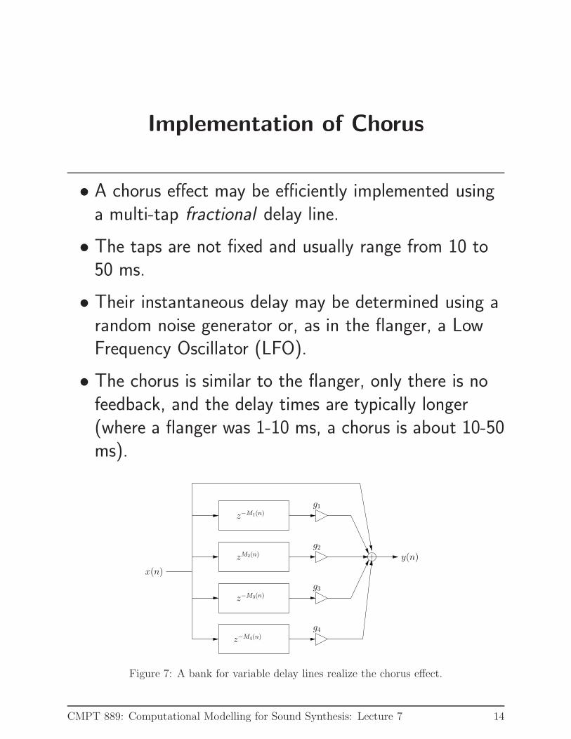
• A chorus effect may be efficiently implemented usinga multi-tap fractional delay line.

• The taps are not fixed and usually range from 10 to50 ms.

• Their instantaneous delay may be determined using arandom noise generator or, as in the flanger, a LowFrequency Oscillator (LFO).

• The chorus is similar to the flanger, only there is nofeedback, and the delay times are typically longer(where a flanger was 1-10 ms, a chorus is about 10-50ms).

z−M1(n)

zM2(n)

z−M3(n)

z−M4(n)

x(n)

y(n)

g2

g1

g3

g4

Figure 7: A bank for variable delay lines realize the chorus effect.


Reverberation

• Reverberation is produced naturally by the reflectionof sounds off surfaces; it’s effect on the overall soundthat reaches the listener depends on the room orenvironment in which the sound is played.

• The amount and quality of reverb depends on

– the volume and dimensions of the space,

– and the type, shape and number of surfaces thatthe sound encounters.

L

S

Figure 8: Example reflection paths occurring between source and listener.


Reflections

• There are several paths the sound emanating from thesource can take before reaching the listener, only oneof which is direct.

• The listener receives many delayed images of thesound reflected from the walls, ceiling and floor of theroom, which lengthen the time the listener hears thesound.

• Since the amplitude of the sound decreases at a rateinversely proportionate to the distance traveled, thesound is not only delayed, but is also at a loweramplitude. Reverb therefore tends to have a decayingamplitude envelope.

• Four physical measurements that effect the characterof reverb are:

1. Reverb time

2. The frequency dependence of reverb time

3. The time delay between the arrival of the directsound and the first reflection

4. The rate at which the echo density builds.


1.Reverb time

• The time required for a sound to die away to 1/1000(-60dB).

• Proportional to how long a listener will hear a sound,but depends also on other factors such as theamplitude of the original sound and the presence ofother sounds.

• Depends on the volume of the room and the nature ofits reflective surfaces. Rooms with large volume tendto have long reverberation times. With a constantvolume, reverb time will decrease with either anincrease in surface area available for reflection.

• Depends on absorptivity of the surfaces. All materialsabsorb some acoustic energy. Hard, solid nonporoussurfaces reflect efficiently whereas soft ones (such ascurtains) absorb more substantially.

• Depends on the roughness of the surfaces. If thesurface is not perfectly flat, part of the sound isreflected and part is dispersed in other directions.


2. The frequency dependence of reverbtime.

• Reverb time is not uniform over the range of audiblefrequencies. In a well designed concert hall, the lowfrequencies are the last to fade.

• Absorptive materials tend to reflect low-frequencysounds better than high ones.

• Efficient reflectors (such as marble) however, reflectsounds of all frequencies with nearly equal efficiency.

• With small solid objects, the efficiency and thedirection of reflection are both dependent offrequency. This causes frequency-dependentdispersion and hence a major alteration of thewaveform of a sound.


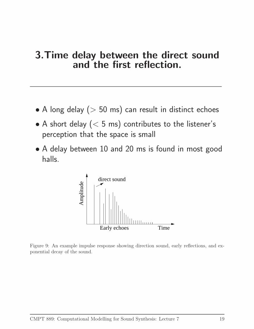
3.Time delay between the direct soundand the first reflection.

• A long delay (> 50 ms) can result in distinct echoes

• A short delay (< 5 ms) contributes to the listener’sperception that the space is small

• A delay between 10 and 20 ms is found in most goodhalls.

Early echoes

Am

plitu

de

direct sound

Time

Figure 9: An example impulse response showing direction sound, early reflections, and ex-ponential decay of the sound.


4.The rate at which the echo densitybuilds

• After the initial reflection, the rate at which theechoes reach the listener begins to increase rapidly.

• A listener can distinguish differences in echo densityup to a density of 1 echo/ms.

• The amount of time required to reach this thresholdinfluences the character of the reverberation. In agood situation, this is typically 100 ms.

• This time is roughly proportional to the square root ofthe volume of a room, so that small spaces arecharacterized by a rapid buildup of echo density.


Digital Reverb

• An electronic reverberator can be thought of as afilter that has been designed to have and impulseresponse emulating the impulse response of the spacebeing simulated.

• Ideally, a digital simulation of a reverberantenvironment permits control over the parameters thatdetermined the character of the reverberation.

• Delay lines can be used to simulate the travel time ofthe indirect sound (reflections) by delaying the soundby the appropriate length of time.

• We can simulate several different amounts of delay ofthe same signal using a single circular delay line, witha length suited for the longest required delay.

• The delay line can by tapped to obtain theappropriate shorter delays, which may varydynamically.

• Convolution is equivalent to tapping a delay line everysample and multiplying the output of each tap by thevalue of the impulse response for that time (thoughthis would be very computationally expensive).


Implementation

• Consider a bank of Feedback Comb filters where eachfilter has a difference equation

y(n) = x(n) + gy(n − M).

• The response decays exponentially as determined bythe loop time M and the coefficient g.

• To obtain a desired reverberation time, g is usuallyapproximated, given the loop time τ , by

g = 0.001τ/T60

where 0.001 is the level of the signal after the reverbtime (the -60dB point) and T60 is the reverb time.

• When unit reverberators are connected in parallel,their impulse responses add. The total number ofpulses produced is the sum of the pulses produced bythe individual units.

• When placed in series (cascade), the impulse responseof one unit triggers the response of the next,producing a much denser response. The number ofpulses produced is the product of the number ofpulses produced by the individual units.


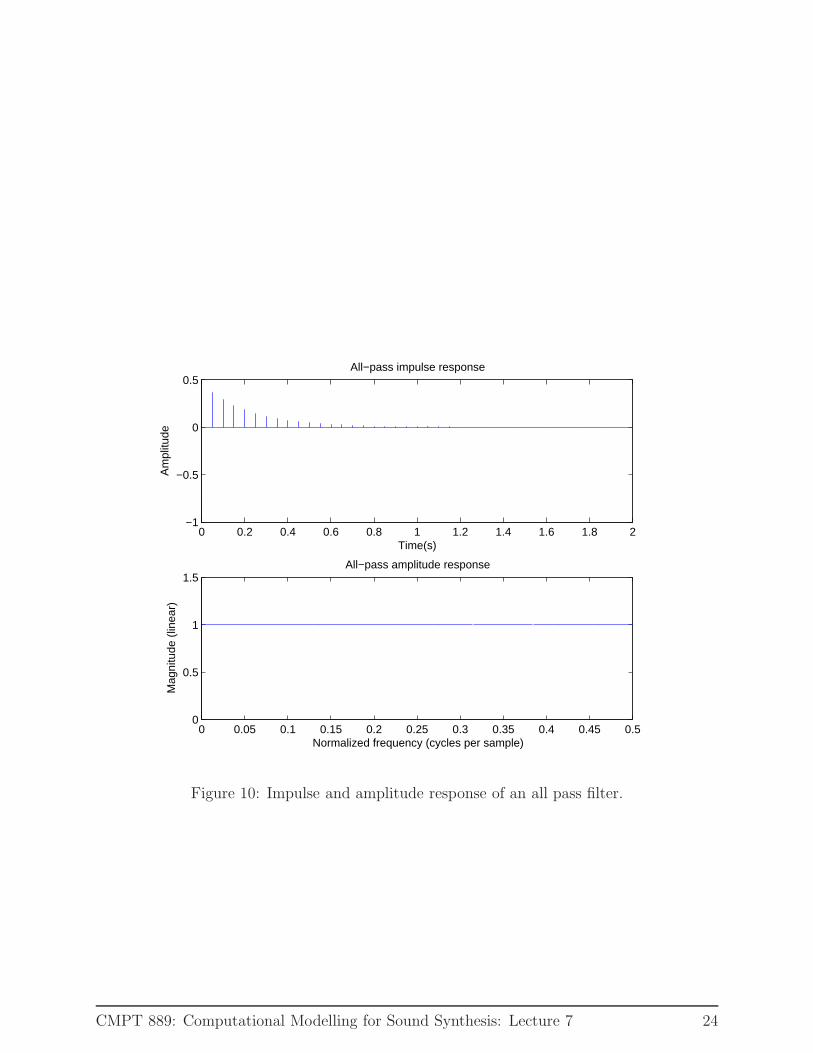
All-pass filters

• Unlike a comb filter, the all-pass filter passes signal ofall frequencies equally. That is, the amplitudes offrequency components are not changed by the filter.

• The all-pass filter however, has substantial effect onthe phase of individual signal components, that is, thetime it takes for frequency components to getthrough the filter. This makes it ideal for modellingfrequency dispersion.

• The effect is most audible on the transient response:during the attack or decay of a sound.

• The difference equation for the all-pass filter is givenby

y(n) = −gx(n) + x(n − M) + gy(n − M).


0 0.2 0.4 0.6 0.8 1 1.2 1.4 1.6 1.8 2−1

−0.5

0

0.5All−pass impulse response

Time(s)

Am

plitu

de

0 0.05 0.1 0.15 0.2 0.25 0.3 0.35 0.4 0.45 0.50

0.5

1

1.5All−pass amplitude response

Normalized frequency (cycles per sample)

Mag

nitu

de (

linea

r)

Figure 10: Impulse and amplitude response of an all pass filter.


Network of unit reverberators

Parallel Connection

• When unit reverberators are connected in parallel,their impulse responses add.

• The total number of pulses produced is the sum ofthe pulses produced by the individual units.

Series Connection

• When placed in series (cascade), the impulseresponse of one unit triggers the response of the next,producing a much denser response.

• The number of pulses produced is the product of thenumber of pulses produced by the individual units.


Two topolgies by Schroeder

x(n) A1

C1

C2

C3

C4

A2 y(n)

Figure 11: Digital reverberator using parallel comb filters and series allpass filters.

A1x(n) y(n)A2 A3 A4 A5

Figure 12: Digital reverberator using series allpass filters.


Choosing control parameter values

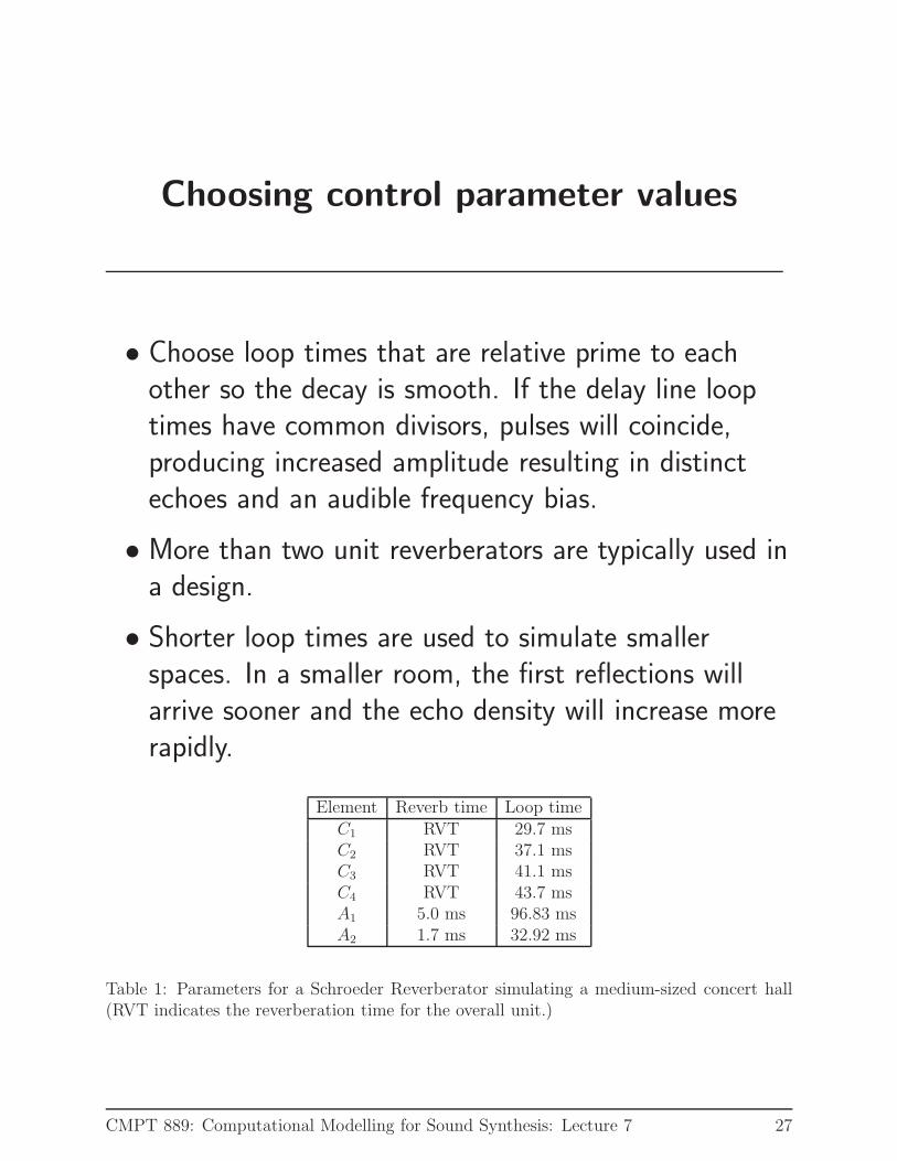
• Choose loop times that are relative prime to eachother so the decay is smooth. If the delay line looptimes have common divisors, pulses will coincide,producing increased amplitude resulting in distinctechoes and an audible frequency bias.

• More than two unit reverberators are typically used ina design.

• Shorter loop times are used to simulate smallerspaces. In a smaller room, the first reflections willarrive sooner and the echo density will increase morerapidly.

Element Reverb time Loop timeC1 RVT 29.7 msC2 RVT 37.1 msC3 RVT 41.1 msC4 RVT 43.7 msA1 5.0 ms 96.83 msA2 1.7 ms 32.92 ms

Table 1: Parameters for a Schroeder Reverberator simulating a medium-sized concert hall(RVT indicates the reverberation time for the overall unit.)


cmpt 889: lecture 7 delay eﬀects: flanging, phasing ...tamaras/effects/effects.pdf · delay...

Documents