Available on the CERN CDS information server CMS PAS HIG-14-009

CMS Physics Analysis Summary

Contact: cms-pag-conveners-higgs@cern.ch 2014/07/03

Precise determination of the mass of the Higgs boson andstudies of the compatibility of its couplings with the

standard model

The CMS Collaboration

Abstract

Properties of the Higgs boson with mass near 125 GeV are measured in proton-protoncollisions with the CMS experiment at the LHC. A comprehensive set of productionand decay measurements are combined. The decays to γγ, ZZ, WW, ττ, and bbpairs are exploited, including studies targeting Higgs bosons produced in associa-tion with a pair of top quarks. The data samples were collected in 2011 and 2012and correspond to integrated luminosities of up to 5.1 fb−1 at 7 TeV and up to 19.7fb−1 at 8 TeV; the final detector calibration and alignment are used in the event re-construction. From the high-resolution γγ and ZZ channels, the mass of this Higgsboson is measured to be 125.03 +0.26

−0.27 (stat.) +0.13−0.15 (syst.) GeV, with the precision domi-

nated by the statistical uncertainty. For this mass, the event yields obtained in thedifferent analyses tagging specific decay modes and production mechanisms are con-sistent with those expected for the standard model Higgs boson. The combinedbest-fit signal strength, relative to the standard model expectation, is found to be1.00 ± 0.09 (stat.) +0.08

−0.07 (theo.) ± 0.07 (syst.) at the measured mass. Various searchesfor deviations in the magnitudes of the Higgs boson scalar couplings from those pre-dicted for the standard model are performed. No significant deviations are found.

1

1 IntroductionOne of the most important objectives of the Large Hadron Collider (LHC) physics programis to understand the mechanism behind electroweak symmetry breaking (EWSB). In the stan-dard model (SM) [1–3] EWSB is achieved by a complex scalar doublet field that leads to theprediction of one physical Higgs boson (H) [4–9].

In 2012 the ATLAS and CMS Collaborations at the LHC reported the observation of a newboson with a mass near 125 GeV [10–13]. Subsequent studies of the production and decayrates [14–24] and of the spin-parity quantum numbers [17, 18, 25, 26] of the new boson showthat its properties are compatible with those expected for the SM Higgs boson.

In proton-proton (pp) collisions at√

s = 7–8 TeV there are four main Higgs boson produc-tion mechanisms predicted by the SM. The gluon-gluon fusion production mode (ggH) has thelargest cross section. It is followed by vector boson fusion (VBF), associated WH and ZH pro-duction (VH), and production in association with top quarks (ttH). The cross section values forthe Higgs boson production modes and the values for the decay branching fractions, togetherwith their uncertainties, are tabulated in Ref. [27] and references therein. For a Higgs bosonmass between 124 GeV and 127 GeV, the total production cross section varies from 17.6 pb to16.2 pb at

√s = 7 TeV, and from 22.4 pb to 21.4 pb at 8 TeV.

The present combination uses the CMS measurements of the properties of this boson targetingits decay to bb [16], WW [17], ZZ [18], ττ [19], and γγ [20], as well as measurements of the ttHproduction mode [14, 28, 29]. For simplicity, bb is used to denote bb, ττ to denote τ+τ−, etc.Similarly, ZZ is used to denote ZZ(∗) and WW to denote WW(∗).

The H → γγ and H → ZZ(∗) → 4` (where ` = e, µ) channels play a special role because ofthe excellent mass resolution of the reconstructed diphoton and four-lepton final states, respec-tively. The H → WW(∗) → `ν`ν measurement has a high sensitivity but relatively poor massresolution because of the presence of neutrinos in the final state. The bb and ττ decay modesare afflicted by large background contributions and have relatively poor mass resolution, mak-ing it challenging to obtain a sensitivity comparable to that of the other channels; combiningthe results from bb and ττ, the CMS Collaboration has published evidence for the decay of thisHiggs boson to fermions [30]. While in the SM the ggH process is dominated by (virtual) top-quark loops, directly probing the coupling of top quarks to this Higgs boson can be achievedby studying events tagged as having been produced via the ttH process.

The mass of the new boson is determined by combining the published measurements of theH→ γγ and H→ ZZ(∗) → 4` channels [18, 20]. The SM Higgs boson is predicted to have spin-parity quantum numbers JP = 0+, and all other properties can be derived if the boson’s massis specified. For the couplings of the Higgs boson to SM particles, we use the combination of allmeasurements to extract ratios between the observed coupling strengths and those predictedby the SM. The formalism used to test for deviations in the magnitudes of the Higgs bosonscalar couplings is that set forth by the LHC Higgs Cross Section Working Group in Ref. [27]and references therein. This formalism assumes, among other things, that the observed statehas JP = 0+ and that the narrow width approximation holds, leading to a factorization of thecouplings in the production and decay of the boson.

The data sets have been processed with the final alignment and calibrations of the CMS detec-tor [31] and correspond to pp collisions collected in 2011 and 2012 with integrated luminositiesof up to 5.1 fb−1 at

√s = 7 TeV and 19.7 fb−1 at 8 TeV. The central feature of the CMS detector

is a 13 m long superconducting solenoid with an internal diameter of 6 m. The solenoid gen-erates a uniform 3.8 T magnetic field parallel to the direction of the LHC beams. Within the

2 2 Analyses entering the combination

superconducting solenoid volume are a silicon pixel and strip tracker, a lead tungstate crystalelectromagnetic calorimeter, and a brass/scintillator hadron calorimeter. Muons are identifiedand measured in gas-ionization detectors embedded in the outer steel magnetic flux returnyoke of the solenoid. The detector is subdivided into a cylindrical barrel and endcap disks oneither side. Calorimeters in the forward and backward directions complement the coverageprovided by the barrel and endcap detectors.

In Section 2 the channels contributing to the combined measurements are summarized. InSection 3 the statistical method used to extract the boson properties is described; some expecteddifferences between the results of the combination and those of the individual analyses are alsoexplained. The results of the present combination are reported in Section 4.

2 Analyses entering the combinationTable 1 provides an overview of all analyses used in this combination, including the followinginformation: the final states selected, the production and decay modes targeted by each anal-ysis, the integrated luminosity used, the expected mass resolution, and the number of eventcategories in each channel.

The following notation is used in Table 1 and throughout the text: σmH /mH is the expectedrelative mass resolution, where σmH is calculated differently in different input analyses; theH → γγ, H → ZZ(∗) → 4`, and H → WW(∗) → `ν`ν analyses quote σmH as half of thewidth of the shortest interval containing 68.3% of the signal events, while the H→ ττ analysisquotes the RMS of the signal distribution. Regarding leptons, ` denotes an electron or a muon,τh denotes a τ lepton identified via its decay into hadrons, and L denotes any charged lep-ton. Regarding lepton pairs, SF denotes same-flavor dileptons and SS (OS) denotes same-sign(opposite-sign) dileptons. Concerning reconstructed jets, CJV denotes a central jet veto, Emiss

Trefers to missing transverse energy, j stands for a reconstructed jet, and b denotes a jet taggedas due to the hadronization of a b quark.

In total, 207 categories are combined, and there are 2519 nuisance parameters corresponding tosources of uncertainty other than those arising from Poisson (counting) statistics.

2.1 H → γγ

The H → γγ analysis [20] measures a narrow signal mass peak over a smoothly falling back-ground due to events originating from prompt non-resonant diphoton production or fromevents with at least one jet misidentified as an isolated photon.

The sample of events with a photon pair is split in mutually exclusive event classes targetingthe different production processes as listed in Table 1. Requiring the presence of two forwardjets favors events produced by the VBF mechanism, while event classes designed to preferen-tially select VH or ttH production require the presence of muons, electrons, Emiss

T , a pair of jetscompatible with the decay of a vector boson, or jets arising from the hadronization of b quarks.For 7 TeV data, there is only one ttH-tagged event class that combines the events selected bythe leptonic ttH and multijet ttH selections. The 2-jet VBF-tagged classes are further split ac-cording to a multivariate (MVA) classifier that is trained to discriminate VBF events from bothbackground and ggH events.

Fewer than 1% of the selected events are tagged according to production mode. The remaining“untagged” events are subdivided into different classes based on the output of an MVA clas-sifier that assigns a high score to signal-like events and to events with a good mass resolution,

2.1 H→ γγ 3

Table 1: Summary of the channels in the analyses included in this combination. The first and secondcolumns indicate which decay mode and/or production mechanism are targeted by an analysis. Noteson the expected composition of the signal are given in the third column. Where relevant, the fourthcolumn specifies the expected relative mass resolution for the SM Higgs boson. Finally, the last columnsprovide the number of categories and the integrated luminosity for the 7 and 8 TeV data sets. Thenotation is explained in the text.

Decay tag and production tag Expected signal composition σmH /mH

Luminosity ( fb−1)No. of categories7 TeV 8 TeV

H→ γγ [20], Section 2.1 5.1 19.7Untagged 76–93% ggH 0.8–2.1% 4 52-jet VBF 50–80% VBF 1.0–1.3% 2 3Leptonic VH ≈95% VH (WH/ZH ≈ 5) 1.3% 2 2Emiss

T VH 70–80% VH (WH/ZH ≈ 1) 1.3% 1 12-jet VH ≈65% VH (WH/ZH ≈ 5) 1.0–1.3% 1 1Leptonic ttH ≈95% ttH 1.1%

1† 1

γγ

Multijet ttH >90% ttH 1.1% 1H→ ZZ(∗) → 4` [18], Section 2.2 5.1 19.7

2-jet 42% VBF + VH 3 34µ, 2e2µ, 4e

Other ≈90% ggH1.3, 1.8, 2.2%‡

3 3H→WW(∗) → `ν`ν [17], Section 2.3 4.9 19.4

0-jet 96–98% ggH eµ: 16%‡ 2 21-jet 82–84% ggH eµ: 17%‡ 2 22-jet VBF 78–86% VBF 2 2

ee + µµ, eµ

2-jet VH 31–40% VH 2 23`3ν WH SF-SS, SF-OS ≈100% WH, up to 20% ττ 2 2

``+ `′νjj ZH eee, eeµ, µµµ, µµe ≈100% ZH 4 4H→ ττ [19], Section 2.4 4.9 19.7

0-jet ≈98% ggH 11–14% 4 41-jet 70–80% ggH 12–16% 5 5eτh, µτh

2-jet VBF 75–83% VBF 13–16% 2 41-jet 67–70% ggH 10–12% - 2

τhτh 2-jet VBF 80% VBF 11% - 10-jet ≈98% ggH, 23–30% WW 16–20% 2 21-jet 75–80% ggH, 31–38% WW 18–19% 2 2eµ

2-jet VBF 79–94% VBF, 37–45% WW 14–19% 1 20-jet 88–98% ggH 4 41-jet 74–78% ggH, ≈17% WW ? 4 4ee, µµ

2-jet CJV ≈50% VBF, ≈45% ggH, 17–24% WW ? 2 2``+ LL′ ZH LL′ = τhτh, `τh, eµ ≈15% (70%) WW for LL′ = `τh (eµ) 8 8`+ τhτh WH ≈96% VH, ZH/WH ≈ 0.1 2 2`+ `′τh WH ZH/WH ≈ 5%, 9–11% WW 2 4

VH with H→ bb [16], Section 2.5 5.1 18.9W(`ν)bb pT(V) bins ≈100% VH, 96–98% WH 4 6W(τhν)bb 93% WH - 1Z(``)bb pT(V) bins ≈100% ZH 4 4Z(νν)bb pT(V) bins ≈100% VH, 62–76% ZH

≈10%

2 3ttH with H→ hadrons [14, 28], Section 2.6 5.0 19.3

tt lepton+jets ≈90% bb but ≈24% WW in ≥6j + 2b 7 7H→ bb

tt dilepton 45–85% bb, 8–35% WW, 4–14% ττ 2 3H→ τhτh tt lepton+jets 68–80% ττ, 13–22% WW, 5–13% bb - 6

ttH with H→ leptons [29], Section 2.6 - 19.62`-SS WW/ττ ≈ 3 - 6

3` WW/ττ ≈ 3 - 24` WW : ττ : ZZ ≈ 3 : 2 : 1 - 1

† Events fulfilling the requirements of either selection are combined into one category.‡ Values for analyses dedicated to the measurement of the mass that do not use the same categories and/or observables.? Composition in the regions for which the ratio between signal and background s/(s + b) > 0.05.

4 2 Analyses entering the combination

based on a combination of i) an event-by-event estimate of the diphoton mass resolution, ii) aphoton identification score for each photon, and iii) kinematic information about the photonsand the diphoton system. The photon identification score is obtained from a separate MVAclassifier that uses shower shape information and variables characterizing how isolated thephoton candidate is to discriminate prompt photons from those arising in jets.

In each event class, the background in the signal region is estimated from a fit to the observeddiphoton mass distribution in data. The uncertainty due to the choice of background func-tional form is incorporated into the statistical procedure; the likelihood maximization is alsoperformed for a discrete variable that selects which of the functional forms is evaluated. Thisprocedure was found to have correct coverage probability and negligible bias in extensive testsusing pseudo-data extracted from fits of multiple families of functional forms to the data. Byconstruction, this “discrete profiling” of the background functional form leads to confidenceintervals on any estimated parameter that are at least as large as those obtained when con-sidering any single functional form. Parameters related to the background functional formscontribute to the statistical uncertainty of measurements.

Three cross-check analyses corroborate the main results. As an alternative to the use of MVAalgorithms, an analysis using simpler selections but the same background treatment is per-formed. An analysis using sidebands is used to cross-check the background treatment. Finally,to cross-check the conclusions regarding VBF production, a two-dimensional analysis usingthe diphoton and dijet masses was developed.

The same event classes and observables are used for the mass measurement and to search fordeviations in the magnitudes of the Higgs boson scalar couplings.

2.2 H → ZZ

In the H→ ZZ(∗) → 4` analysis [18], we measure a four-lepton mass peak over a small contin-uum background. To further separate signal and background, we build a discriminant, Dkin

bkg,

using the leading order matrix elements for signal and background. The value of Dkinbkg is cal-

culated from the observed kinematics, namely the masses of the two dilepton pairs and fiveangles, which uniquely define a four-lepton configuration in their center-of-mass frame.

Given the different mass resolutions and different background rates arising from jets misiden-tified as leptons, the 4e, 4µ, and 2e2µ event categories are analyzed separately.

The dominant irreducible background in this channel is due to non-resonant ZZ productionwith both Z bosons decaying to a pair of charged leptons and is estimated from simulation.The smaller reducible backgrounds with misidentified leptons, mainly from the production ofZ + jets, tt, and WZ + jets, are estimated from data.

To increase the sensitivity to the production mechanism, the event sample is split into two cat-egories based on jet multiplicity: i) events with fewer than two jets, and ii) events with at leasttwo jets. In the first category, the four-lepton transverse momentum is used to discriminateVBF and VH production from ggH. In the second category a linear discriminant, built from theinvariant mass of the two leading jets and their pseudorapidity difference, is used to separatethe VBF and ggH processes.

For the mass measurement an event-by-event estimator of the mass resolution is built from thesingle-lepton momentum resolutions evaluated from the study of a large number of J/ψ→ µµand Z→ `` data events. The relative mass resolution, σm4`/m4`, is then used together with m4`and Dkin

bkg to measure the boson mass.

2.3 H→WW 5

2.3 H → WW

In the H→WW(∗) → `ν`ν analysis [17], we measure an excess of events with two oppositely-charged leptons or three leptons with a total charge of ±1, moderate Emiss

T , and up to two jets.

The two-lepton events are divided into six categories, with different background compositionsand signal-to-background ratios. For events with no jets, the main background is due to non-resonant WW production; for events with one jet, the dominant backgrounds are from WW andtop-quark production. The events are split into same-flavor and different-flavor dilepton eventcategories, since the background from Drell–Yan production (qq → γ∗/Z(∗) → ``) is muchlarger for same-flavor dilepton events. The 2-jet VBF tags are optimized to take advantage ofthe VBF production signature. The main background is from top-quark production. The 2-jetVH tag targets the decay of the vector boson into two jets, V → jj. The selection requires twocentrally-produced jets with invariant mass in the range 65 < mjj < 105 GeV. To reduce the top-quark, Drell–Yan, and WW backgrounds, a selection is performed on the dilepton mass and onthe angular separation between the leptons. All background rates, except for very small con-tributions from WW, ZZ, and Wγ, are evaluated from data. The two-dimensional distributionof events in the (m``, mT) plane, where m`` is the invariant mass of the dilepton pair and mT isthe transverse mass reconstructed from the transverse momentum of the dilepton pair and theEmiss

T vector, is used for the measurements in the different-flavor dilepton categories with zeroand one jets. For the same-flavor dilepton categories and for the 2-jet VH tag analysis only theevent totals are used.

In the 3`3ν channel tagging WH → WWW, we search for an excess of events with three lep-tons, electrons or muons, large Emiss

T , and low hadronic activity. The dominant background isfrom WZ → 3`ν production, which is largely reduced by requiring that all same-flavor andoppositely-charged lepton pairs have a dilepton mass away from the Z boson mass. The small-est distance between the oppositely-charged leptons is the observable chosen to perform themeasurement. The background processes with jets misidentified as leptons, e.g., Z + jets andtop production, as well as the WZ → 3`ν background are estimated from data. The smallcontribution from the ZZ → 4` process with one of the leptons having escaped detection isestimated using simulated samples.

In the 3`νjj channel targeting ZH → Z + WW → ``+ `νjj, we first identify the leptonic decayof the Z boson and then require the dijet system to satisfy |mjj −mW| ≤ 60 GeV. The transversemass of the `νjj system is the observable chosen to perform the measurement. The main back-grounds are due to the production of WZ, ZZ, and tri-bosons, as well as processes involvingnon-prompt leptons. The first three are estimated from simulated samples, while the last oneis evaluated from data. It should be noted that in the 3`3ν channel up to 20% of the decays aredue to H→ ττ. This contribution is negligible in the 3`νjj channel.

Finally, a dedicated analysis for the measurement of the mass is performed in the 0-jet and 1-jet categories of the eµ channel. Employing observables which are extensively used in SUSYsearches, a resolution of 16–17% for mH = 125 GeV has been achieved.

2.4 H → ττ

The H→ ττ analysis [19] measures an excess of events using multiple final-state signatures in-cluding the eµ, eτh, µτh, and τhτh final states, where electrons and muons arise from leptonic τdecays. The samples are further divided into categories based on the number of reconstructedjets in the event: 0 jets, 1 jet, or 2 jets. The 0-jet and 1-jet categories are further subdivided ac-cording to the reconstructed pT of the leptons. The 2-jet categories require a VBF-like topology

6 2 Analyses entering the combination

and are subdivided according to selection criteria applied to the dijet kinematic properties. Ineach of these categories, we search for a broad excess in the reconstructed ττ mass distribution.The 0-jet category is used to constrain background normalizations, identification efficiencies,and energy scales. Various control samples in data are used to evaluate the main irreduciblebackground from Z→ ττ production and the largest reducible backgrounds from W+ jets andmultijet production.

The ee and µµ final states are similarly subdivided into categories as above but given the twoneutrinos present in the final state the search is performed on the combination of two MVAdiscriminants. The first is trained to distinguish Z → `` events from Z → ττ events while thesecond is trained to separate Z→ ττ events from H→ ττ events.

The search for H → ττ decays produced in association with a W or Z boson is conductedin events with three or four leptons in the final state. The analysis targeting WH productionselects events that have electrons or muons and one or two hadronically-decaying tau leptons:µ+ µτh, e+ µτh or µ+ eτh, µ+ τhτh, and e+ τhτh. The analysis targeting ZH production selectsevents with an identified Z → `` decay and a Higgs boson candidate decaying to eµ, eτh, µτh,or τhτh. The main irreducible backgrounds to the WH and ZH searches are WZ and ZZ dibosonevents, respectively. The irreducible backgrounds are estimated using simulated event samplescorrected by measurements from control samples in data. The reducible backgrounds in bothanalyses are W, Z, and tt events with at least one jet misidentified as an isolated e, µ, or τh.These backgrounds are estimated exclusively from data by measuring the probability for jetsto be misidentified as isolated leptons in background-enriched control regions, and weightingthe selected events that fail the lepton requirements with the misidentification probability. Forthe SM Higgs boson, the expected fraction of H → WW events in the ZH analysis is 10–15%for ZH→ Z + `τh and 70% for ZH→ Z + eµ.

2.5 VH with H → bb

Exploiting the large expected H → bb branching fraction, the analysis of VH production andH→ bb decay examines the W(`ν)bb, W(τhν)bb, Z(``)bb, and Z(νν)bb topologies [16].

The Higgs boson candidate is reconstructed by requiring two b-tagged jets. The event sampleis divided into classes depending on the transverse momentum of the vector boson, pT(V).An MVA regression is used to estimate the true b-quark energy after being trained on recon-structed b-jets in simulated H → bb events. This regression achieves a final dijet mass resolu-tion of about 10% for mH = 125 GeV. The performance of the regression algorithm is checkedwith data where it is observed to improve the top-quark mass measurement in tt events and toimprove the pT balance between a Z boson and b-quark jets in Z(→ ``) + bb events. Eventswith higher pT(V) have smaller backgrounds and better dijet mass resolution. A cascade ofMVA classifiers, trained to distinguish the signal from tt, V + jets, and diboson events, im-proves the sensitivity in the W(`ν)bb, W(τhν)bb, and Z(νν)bb channels. The rates of the mainbackgrounds, consisting of V+ jets and tt events, are derived from signal-depleted data controlsamples. The WZ and ZZ backgrounds where Z → bb, as well as the single-top-quark back-ground, are estimated from simulated samples. The MVA classifier output distribution is usedas the final discriminant in performing measurements.

2.6 ttH-production analyses

Given its distinctive signature, the ttH production process can be tagged using the decay prod-ucts of the tt pair. The search for ttH production is performed in three channels: H → bb [28],H→ τhτh [28], and H→ leptons [29].

7

In the analysis of ttH production with H → bb, two signatures for the tt pair decay are con-sidered: lepton-plus-jets (tt → `νjjbb) and dilepton (tt → `ν`νbb). In the analysis of ttH pro-duction with H → τhτh, the tt lepton-plus-jets decay signature is required. In both channels,the events are further classified according to the numbers of jets and b-tagged jets identified.The major background is from top-pair production accompanied by extra jets. An MVA istrained to discriminate between background and signal events using information related to re-constructed object kinematics, event shape, and the discriminant output from the b-quark-jettagging algorithm. The rates of background processes are estimated from simulated samplesand are constrained through the inclusion of background enriched control samples in the sta-tistical procedure.

The analysis of ttH production and H → leptons is mainly sensitive to the Higgs decays toWW, ττ, and ZZ, with subsequent decay to electrons and/or muons. The selection starts byrequiring the presence of at least two central jets and at least one jet tagged as originating froma b quark. It then proceeds to categorize the events depending on the number, charge, andflavor of the reconstructed leptons: 2` with the same sign, 3` with a total charge of ±1, or 4`. Adedicated MVA lepton selection is used to suppress the reducible background from misiden-tified leptons, usually from the decay of b hadrons. After the final selection, the two mainbackgrounds include one that is due to misidentified leptons, which is evaluated from data,and associated production of tt and vector bosons, which is estimated from simulated samples.Measurements in the 4` event category are performed using the number of reconstructed jets,Nj. In the remaining categories an MVA classifier is employed, which makes use of Nj as wellas other kinematic and event shape variables to discriminate between signal and background.

3 Combination methodologyThe combination of Higgs boson measurements requires the simultaneous analysis of the dataselected by all individual analyses, accounting for all statistical uncertainties, systematic un-certainties, and their correlations.

The overall statistical methodology used in this combination was developed by the ATLASand CMS Collaborations in the context of the LHC Higgs Combination Group and is describedin Refs. [12, 32, 33]. The chosen test statistic q is based on the profile likelihood ratio and isused to determine how signal-like or background-like the data are. Systematic uncertaintiesare incorporated in the analysis via nuisance parameters that are treated according to the fre-quentist paradigm. Below we give concise definitions of statistical quantities that we use forcharacterizing the outcome of the measurements. Results presented in this note are obtainedusing asymptotic formulae [34], including a few updates recently introduced in the RooStatspackage [35].

3.1 Characterizing an excess of events: p-values and significance

To quantify the presence of an excess of events over what is expected for the background,we use the test statistic where the likelihood appearing in the numerator corresponds to thebackground-only hypothesis:

q0 = −2 lnL(data | b, θ0)

L(data | µ · s + b, θ), with µ > 0, (1)

where s stands for the signal expected under the SM Higgs hypothesis, µ is a signal strength

8 3 Combination methodology

modifier introduced to accommodate deviations from SM Higgs predictions, b stands for back-grounds, and θ are nuisance parameters describing systematic uncertainties. The value θ0 max-imizes the likelihood in the numerator under the background-only hypothesis, µ = 0, while µand θ define the point at which the likelihood reaches its global maximum.

The quantity p0, henceforth referred to as the local p-value, is defined as the probability, underthe background-only (b) hypothesis, to obtain a value q0 at least as large as that observed indata, qdata

0 :

p0 = P(

q0 ≥ qdata0

∣∣∣ b)

. (2)

The local significance z of a signal-like excess is then computed from the following equation,using the one-sided Gaussian tail convention:

p0 =∫ +∞

z

1√2π

exp(−x2/2) dx. (3)

Note that very small p-values should be interpreted with caution as the systematic biases anduncertainties in the underlying model are only known with finite precision.

3.2 Extracting signal model parameters

Signal model parameters a, such as the signal strength modifier µ, are evaluated from scans ofthe profile likelihood ratio q(a):

q(a) = −2 ∆ lnL = −2 lnL(data | s(a) + b, θa)

L(data | s(a) + b, θ). (4)

The parameters a and θ correspond to the global maximum likelihood and are called the best-fitset.

The post-fit model, obtained after the signal-plus-background fit to the data, corresponds to theparametric bootstrap described in the statistics literature, includes information gained in the fitregarding the values of all parameters [36, 37], and is used when deriving expected quantities.

The 68% and 95% confidence level (CL) intervals for a given parameter of interest ai are eval-uated from q(ai) = 1.00 and q(ai) = 3.84 respectively, with all other unconstrained model pa-rameters treated in the same way as the nuisance parameters. The two-dimensional (2D) 68%and 95% CL contours for pairs of parameters are derived from q(ai, aj) = 2.30 and q(ai, aj) =6.99, respectively. One should keep in mind that boundaries of 2D confidence regions projectedon either parameter axis are not identical to the one-dimensional (1D) confidence interval forthat parameter.

All results are given using the chosen test statistic result in approximate CL intervals or regions.

3.3 Grouping of channels by decay tag and by production tag

The event samples selected by the different analyses are mutually exclusive. The selectioncriteria can, in most cases, define pure selections of the targeted decay or production modes.For instance, the ttH-tagged event classes of the H → γγ analysis are pure in terms of γγdecays and are expected to contain less than 10% of non-ttH events.

3.4 Expected differences with respect to the results of input analyses 9

Unfortunately, in some cases such pure compositions are not achievable for both productionand decay tags. Mixed production mode composition is common in VBF-tagged event classeswhere the ggH contribution can be as high as 50%, or in VH tags where WH and ZH mixturesare common. On the decay side, mixed composition is more marked for signatures involvinglight leptons and Emiss

T , where both the H→WW and H→ ττ decays may contribute. This canbe seen in Table 1, where some VH-tag analyses targeting H → WW decays have a significantcontribution from H→ ττ decays and vice versa. This is also the case of the eµ channel in theH→ ττ analysis, in particular in the 2-jet VBF tag categories, where the contribution from H→WW decays is sizable and concentrated at low values of mττ, entailing a genuine sensitivity ofthese categories to H→WW decays. On the other hand, in the ee and µµ channels of the H→ττ analysis, the contribution from H→WW is large when integrated over the full range of theMVA observable used, but given that the analysis was optimized for ττ decays the contributionfrom H→ WW is not concentrated in the regions with largest signal-to-background ratio, andprovides little added sensitivity.

Another case of mixed decay composition is that of the analyses targeting ttH production,where the H → leptons decay selection includes sizable contributions from H → WW andH → ττ decays, and to a lesser extent also from H → ZZ decays. The mixed composition isa consequence of designing the analysis to have the highest possible sensitivity to the ttH pro-duction mode. The analysis of ttH with H → τhτh decay has a composition that is dominatedby H → ττ decays, followed by H → WW decays, and a smaller contribution of H → bbdecays. Finally, in the analysis of ttH with H → bb, there is an event class of the lepton + jetschannel that requires six or more jets and two b-tagged jets where the signal is expected to be58% from H → bb, 24% from H → WW, and the remaining 18% from the other SM decaymodes; in the dilepton channel, the event class requiring four or more jets and two b-taggedjets is expected to contain 45% from H→ bb, 35% from H→WW, and 14% from H→ ττ.

When results are grouped according to decay tag, each individual category is assigned to thedecay mode group that, in the SM, is expected to dominate the sensitivity in that channel. Inparticular,

H→ γγ tagged includes only categories from the H→ γγ analysis of Ref. [20].

H→ ZZ tagged includes only categories from the H→ ZZ analysis of Ref. [18].

H→WW tagged includes all the channels from the H → WW analysis of Ref. [17] and thechannels from the analysis of ttH with H→ leptons of Ref. [29].

H→ ττ tagged includes all the channels from the H → ττ analysis of Ref. [19] and the chan-nels from the analysis of ttH targeting H→ τhτh of Ref. [28].

H→ bb tagged includes all the channels of the analysis of VH with H → bb of Ref. [16] andthe channels from the analysis of ttH targeting H→ bb of Refs. [14, 28].

When results are grouped by production tag, the same reasoning of assignment by preponder-ance of composition is followed, using the information in Table 1.

3.4 Expected differences with respect to the results of input analyses

The grouping of channels described in Section 3.3 is among the reasons why the results ofthe combination may differ from those of the individual published analyses. In addition, thecombined measurement takes into account correlations among several sources of systematic

10 4 Results

uncertainty. Care is taken to understand the post-fit behavior of the parameters that are corre-lated between analyses. Finally, the combination is evaluated at a value of mH that is not thevalue that has been used in some of the individual published analyses, entailing changes to theexpected cross section and branching fractions for the SM Higgs boson. Changes are sizable insome cases.

The following differences are easily understood:

• In Refs. [17, 18] the results for H → ZZ(∗) → 4` and H → WW(∗) → `ν`ν areevaluated for mH = 125.6 GeV, the mass measured in the H → ZZ(∗) → 4` anal-ysis. In the present combination the results are evaluated for mH = 125.0 GeV, thecombined mass measurement from the H → γγ and H → ZZ(∗) → 4` analyses.For values of mH in this region, the branching fractions for H → ZZ(∗) → 4` andH → WW(∗) → `ν`ν vary rapidly with mH. For the change of mH in question,B(H → ZZ(∗) → 4`) drops by 5% (relative) and B(H → WW(∗) → `ν`ν) drops by4% (relative) [27]. Therefore, when measuring the signal strength relative to the SMexpectation, an immediate increase of the same order is expected.

• The H→ ττ analysis of Ref. [19] focused on exploring the coupling of the tau leptonto the Higgs boson. For this reason nearly all results in Ref. [19] were obtained bytreating the H → WW contribution as a background, set to the SM expectation.In the present combination, both the H → ττ and H → WW contributions areconsidered as signal in the ττ decay tag analysis, leading to an increased sensitivityto the presence of a Higgs boson.

4 ResultsIn this section the results of the combination are presented. We first present a precise measure-ment of the mass of the new boson using the high-resolution H → γγ and H → ZZ(∗) → 4`channels. Next, we assess the significance of the observed excesses at the best-fit mass value.Finally, we evaluate the consistency of the data observed in the different channels with theexpectations for a SM Higgs boson with mass equal to the mass of the observed boson.

4.1 Mass of the observed state

To measure the mass of the observed state, we use the H → ZZ(∗) → 4` and γγ channels,which have excellent mass resolution. Figure 1 shows 2D 68% CL regions for two parametersof interest, the signal strength relative to the SM expectation, µ = σ/σSM, and the mass, mH,based on these channels. The combined 68% CL confidence region, bounded by a black curvein Fig. 1, is calculated assuming the SM Higgs boson relative event yields between the twochannels, while the overall signal strength is left as a free parameter.

To extract the value of mH in a way that is not completely dependent on the SM relative produc-tion and decay ratios, the signal strength modifiers for the (ggH, ttH)→ γγ, (VBF, VH)→ γγ,and pp→ H→ ZZ(∗) → 4` processes are assumed to be independent and therefore not tied tothe SM expectation. The signal in all channels is assumed to be due to a single state with massmH. The best-fit value of mH and its uncertainty are extracted from a scan of the combined teststatistic q(mH) with the three signal strength modifiers profiled together with all other nuisanceparameters. Figure 2 (left) shows the scan of the test statistic as a function of the mass mH sep-arately for the two channels and for their combination. The intersections of the q(mH) curveswith the thick horizontal line at 1.00 and thin line at 3.84 define the 68% and 95% CL intervalsfor the mass of the observed particle, respectively. These intervals include both the statistical

4.1 Mass of the observed state 11

(GeV)Hm123 124 125 126 127

SM

σ/σ

0.0

0.5

1.0

1.5

2.0

Combined

taggedγγ →H

ZZ tagged→H

CMSPreliminary

(7 TeV)-1 (8 TeV) + 5.1 fb-119.7 fb

ZZ→ + H γγ →H

Figure 1: The 68% CL contours for the signal strength σ/σSM versus the boson mass mH forthe γγ (green) and 4` (red) final states, and their combination (black). The symbol σ/σSMdenotes the production cross section times the relevant branching fractions, relative to the SMexpectation. In this combination, the relative signal strength for the two decay modes is set tothe expectation for the SM Higgs boson.

(GeV)Hm123 124 125 126 127

ln L

∆-

2

0

1

2

3

4

5

6

7

8

9

10Combined

taggedγγ →H

ZZ tagged→H

Combined taggedγγ →H

ZZ tagged→H

CMSPreliminary

(7 TeV)-1 (8 TeV) + 5.1 fb-119.7 fb

ZZ→ + H γγ →H (ggH,ttH),

γγµ,

ZZµ

(VBF,VH)γγ

µ

(GeV)4lH - mγγ

Hm-2.5 -2 -1.5 -1 -0.5 0

ln L

∆-

2

0

1

2

3

4

5

6

7

8

9

10CMSPreliminary

(7 TeV)-1 (8 TeV) + 5.1 fb-119.7 fb

ZZ→ + H γγ →H (ggH,ttH),

γγµ,

ZZµ

(VBF,VH)γγ

µ

Figure 2: (Left) Scan of the test statistic q(mH) = −2 ∆ lnL versus the boson mass mH for the γγ(green) and 4` (red) final states separately and for their combination (black). Three independentsignal strengths, (ggH, ttH)→ γγ, (VBF, VH)→ γγ, and pp→ H→ ZZ(∗) → 4`, are profiledtogether with all other nuisance parameters. (Right) Scan of the test statistic q(mγγ

H − m4`H )

versus the difference between two individual mass measurements for the same model used inthe left panel.

12 4 Results

and systematic uncertainties. The mass is measured to be mH = 125.03+0.29−0.31 GeV. To quantify

the compatibility of the two individual measurements with each other, we perform a scan ofthe test statistic q(mγγ

H −m4`H ), as a function of the difference between two mass measurements.

There are two degrees of freedom in this test, namely the mass difference and mγγH , which is

profiled in the scan. The result is mγγH − m4`

H = −0.87+0.54−0.59 GeV and is shown in Fig. 2 (right);

the two measurements agree at the 1.6σ level.

To evaluate the statistical component of the overall uncertainty, we also perform a scan ofq(mH) fixing all nuisance parameters to their best-fit values, except for those related to theH → γγ background models; given how the H → γγ background distributions are modeledfrom fits to data, their degrees of freedom encode fluctuations which are statistical in nature.The result is shown by the dashed curve in Fig. 3. The crossings of the dashed curve with thethick horizontal line define the 68% CL interval for the statistical uncertainty in the mass mea-surement: +0.26

−0.27 GeV. We derive the systematic uncertainty assuming that the total uncertaintyis the sum in quadrature of the statistical and systematic components; the full result can bewritten as mH = 125.03 +0.26

−0.27 (stat.) +0.13−0.15 (syst.) GeV. The expected uncertainty is evaluated us-

ing an Asimov pseudo-data set [34] constructed from the best-fit values obtained when testingfor the compatibility of the mass measurement in the H → γγ and H → ZZ(∗) → 4` chan-nels. The expected uncertainty thus derived is +0.26

−0.25 (stat.) ± 0.14 (syst.) GeV, in good agree-ment with the observation in data. As a comparison, the expected uncertainty is also derivedby constructing an Asimov pseudo-data set as above except that the signal strength modifiersare set to unity (as expected in the SM), mγγ

H = 125 GeV, and mγγH − m4`

H = 0 GeV, leading to±0.28 (stat.) ± 0.13 (syst.) GeV. As could be anticipated, the statistical uncertainty is slightlylarger given that the observed signal strength in the H → γγ channel is larger than unity, andthe systematic uncertainty is slightly smaller given the small observed mass difference betweenthe two channels.

To assess the dependency of the mass measurement on the SM Higgs boson hypothesis, themeasurement is repeated using the same channels, but with the following two sets of assump-tions: i) allowing a common signal strength modifier to float, which corresponds to the resultin Fig. 1, and ii) constraining the relative production cross sections and branching fractions tothe SM predictions, i.e., µ = 1. The results from these two alternative measurements differby less than 0.1 GeV with respect to the main result, both in terms of the best-fit value and theuncertainties.

4.2 Significance of the observed excess

Table 2 summarizes the median expected and observed local significance for a SM Higgs bosonmass of 125.0 GeV from the different decay mode tags, grouped as described in Section 3.3.The value of mH is fixed to the best-fit combined measurement presented in Section 4.1. Theexpected significance values are evaluated using the post-fit expected background rates andthe signal rates expected from the SM. The ±1σ range around the median significance containsapproximately 68% of the statistical fluctuations that could occur in data, except for the ZZchannel; given the high signal-to-background ratio in the ZZ channel, 68% of the statisticalfluctuations that could occur in data are contained in a range of ±1.4σ around the medianexpected significance.

In each decay group the probability is low for a statistical fluctuation of the background toproduce an excess at least as large as that observed. Differences between the results Table 2and the individual publications are understood in terms of the discussion in Sections 3.3 and3.4, namely the grouping of channels by decay mode tag, the change of mH for which the

4.2 Significance of the observed excess 13

(GeV)Hm123 124 125 126 127

ln L

∆-

2

0

1

2

3

4

5

6

7

8

9

10stat. + syst.

stat. only

CMSPreliminary

(7 TeV)-1 (8 TeV) + 5.1 fb-119.7 fb

ZZ→ + H γγ →H (ggH,ttH),

γγµ,

ZZµ

(VBF,VH)γγ

µ

Figure 3: Scans of the test statistic q(mH) versus the boson mass mH for the combination ofthe γγ and 4` analyses. The solid curve is obtained by profiling all nuisance parameters andthus includes both statistical and systematic uncertainties, as in Fig. 2 (left). The dashed curve isobtained by fixing all nuisance parameters to their best-fit values, except for those related to theH → γγ background description, thus including only statistical uncertainties. The crossingswith the thick (thin) horizontal lines define the 68% (95%) CL interval for the measured mass.

Table 2: The median observed and expected significances of the excesses for mH = 125.0 GeVof the combinations of decay mode groups. The channels are grouped by decay mode tag asdescribed in Section 3.3; when there is a difference in the channels included with respect tothe published results for the individual channels, the result for the grouping used in thosepublications is also given.

Channel groupingSignificance (σ)

Observed ExpectedH→ ZZ tagged 6.5 6.3H→ γγ tagged 5.6 5.3H→WW tagged 4.7 5.4

Grouped as in Ref. [17] 4.3 5.4H→ ττ tagged 3.8 3.9

Grouped as in Ref. [19] 3.9 3.9H→ bb tagged 2.0 2.3

Grouped as in Ref. [16] 2.1 2.3

14 4 Results

significance of the H → ZZ(∗) → 4` and H → WW(∗) → `ν`ν analyses is evaluated, and thetreatment of H→WW as part of the signal, instead of background, in the H→ ττ analysis.

Finally, the γγ and H → ZZ(∗) → 4` decay modes indicate that the new particle is a boson,and the diphoton decay implies that its spin is different from unity [38, 39]. The observeddata have been shown to disfavor spin-2 hypotheses and, assuming that the boson has zerospin, to be consistent with the pure scalar hypothesis, while disfavoring the pure pseudoscalarhypothesis [17, 18].

4.3 Compatibility of the observed state with the SM Higgs boson hypothesis

The size of the current data set allows only a limited number of compatibility tests of the ob-served excesses with the expected SM signal. These tests are presented in this subsection.These compatibility tests do not constitute measurements of any physics parameters per se,but rather probe the consistency of the various observations with the expectations for the SMHiggs boson.

4.3.1 Signal strength in combination and subcombinations

The best-fit value for the common signal strength modifier µ = σ/σSM, obtained in the combi-nation of all search channels, provides the first compatibility test. In the formal fit, µ is allowedto become negative if the observed number of events is smaller than the expected yield for thebackground-only hypothesis. The observed µ value for a Higgs boson mass mH = 125.0 GeVis 1.00± 0.13, consistent with unity, as expected for the SM Higgs boson by construction. Theuncertainty can be further broken down into a statistical component (stat.), a component as-sociated with QCD scale variations, parton distribution functions, branching fractions, un-derlying event description (theo.), and any other systematic uncertainties (syst.); the result is1.00 ± 0.09 (stat.) +0.08

−0.07 (theo.) ± 0.07 (syst.).

Figure 4 shows the µ values obtained in different subcombinations of channels for mH =125.0 GeV, grouped by predominant decay mode or by additional tags targeting events fromparticular production mechanisms. As discussed in Section 3.3 the expected purities of the dif-ferent tagged samples vary substantially. Therefore, these plots cannot be interpreted literallyas compatibility tests for pure production mechanisms or decay modes. The mix of produc-tion and decay modes is naturally handled in terms of deviations in the magnitudes of the SMHiggs boson scalar couplings, presented in Section 4.3.2.

The level of compatibility of any subcombination with the SM Higgs boson cross section canbe quantified by the value of the test statistic

qµ = −2 ∆ lnL = −2 lnL(data | µ, θµ)

L(data | µ, θ)(5)

at µ = 1, which, asymptotically in the limit of large statistics, has a χ2 distribution. For N sub-combinations, the sum of the individual qµ(µ = 1) values is expected to behave asymptoticallyas a χ2 distribution with N degrees of freedom (dof).

The sixteen subchannel combination shown in Fig. 4 (top) gives a χ2/(dof) = 10.5/16, whichcorresponds to an asymptotic p-value of 0.84. The five subcombinations by decay mode tagshown in Fig. 4 (bottom left) yield a χ2/(dof) = 0.9/5 and an asymptotic p-value of 0.97. Fig-ure 4 (bottom right) shows an excess in the ttH-tagged subcombination, due to the observationsin the ttH-tagged H→ γγ and H→ leptons analyses that can be seen in the top panel. The sub-

4.3 Compatibility of the observed state with the SM Higgs boson hypothesis 15

Table 3: The best-fit values for the signal strength at mH = 125.0 GeV, of the VBF and VH, andof the ggH and ttH production mechanisms, µVBF,VH and µggH,ttH, respectively. The channelsare grouped by decay mode tag as described in Section 3.3. The observed and median expectedresults for the ratio of µVBF,VH to µggH,ttH together with their uncertainties are also given for thefull combination.

Channel grouping Best fit (µggH,ttH, µVBF,VH)

H→ ZZ tagged (0.88, 1.75)H→ γγ tagged (1.07, 1.24)H→WW tagged (0.87, 0.66)H→ ττ tagged (0.52, 1.21)H→ bb tagged (0.57, 0.96)

Combined best fit µVBF,VH/µggH,ttH

Observed (expected)1.25+0.63

−0.45 (1.00+0.49−0.35)

combinations by production process tag have a χ2/(dof) = 5.3/4 and an asymptotic p-value of0.26, clearly driven by the excess observed in the analyses tagging the ttH production process.

The p-values above indicate that the extracted signal strengths in these subcombinations arecompatible with the SM prediction for the Higgs boson, µ = 1. The result of the ttH-taggedsubcombination is compatible with the SM hypothesis at the 2.0σ level.

The four main Higgs boson production mechanisms can be associated with either fermion cou-plings (ggH and ttH) or vector-boson couplings (VBF and VH) of the Higgs boson. Therefore,a combination of channels associated with a particular decay mode tag, but explicitly targetingdifferent production mechanisms, can be used to test the relative strengths of the couplingsto the vector bosons and fermions (mainly the top quark). The categorization of the differentchannels into production mode tags is not pure and contributions from the different signal pro-cesses are evaluated from Monte Carlo simulation and taken into account in the fits. Figure 5(left) shows the 68% CL confidence regions for the signal strength modifiers associated withthe ggH and ttH, and with the VBF and VH production mechanisms, µggH,ttH and µVBF,VH, re-spectively. The five sets of contours correspond to the five combinations by predominant decaymode as presented in Table 2. The SM Higgs boson expectation of (1, 1) is within the 68% CLregions in all cases. The best-fit values for each decay mode group are given in Table 3.

The ratio of µVBF,VH and µggH,ttH can also be measured in each decay mode group. In this ratiothe branching fractions cancel out in each channel and the results of the different channels canbe combined. Figure 5 (right) shows the corresponding likelihood scan of the data for this ratio.

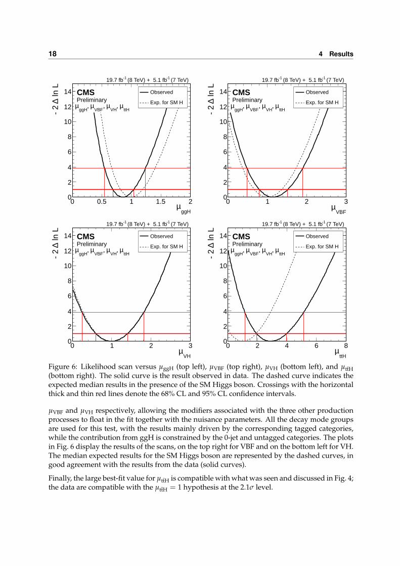
Figure 6 shows the results of scans of four independent signal strengths corresponding to thefour SM main production processes, assuming the relative branching fractions of the SM; thebest-fit results are given in Table 4. From the scan on the top left, the µggH best-fit value isfound to be 0.85+0.19

−0.17. After calculating the component of the uncertainty that is statistical innature (stat.) and that which is related to the theory inputs (theo.), one can then subtract themin quadrature from the total uncertainty and assign the remainder as systematic uncertainty(syst.), yielding 0.85 +0.11

−0.09 (stat.) +0.11−0.08 (theo.) +0.10

−0.09 (syst.).

It is also interesting to probe the vector-boson production mechanisms and assess indepen-dently the signal strengths for the VH and VBF modes. Likelihood scans are performed versus

16 4 Results

SMσ/σBest fit -4 -2 0 2 4 6

ZZ (2 jets)→H ZZ (0/1 jet)→H

(ttH tag)ττ →H (VH tag)ττ →H

(VBF tag)ττ →H (0/1 jet)ττ →H

WW (ttH tag)→H WW (VH tag)→H

WW (VBF tag)→H WW (0/1 jet)→H

(ttH tag)γγ →H (VH tag)γγ →H

(VBF tag)γγ →H (untagged)γγ →H bb (ttH tag)→H bb (VH tag)→H

0.13± = 1.00 µ Combined

CMSPreliminary

(7 TeV)-1 (8 TeV) + 5.1 fb-119.7 fb

= 125 GeVH m

SMσ/σBest fit 0 0.5 1 1.5 2

0.29± = 1.00 µ ZZ tagged→H

0.21± = 0.83 µ WW tagged→H

0.24± = 1.13 µ taggedγγ →H

0.27± = 0.91 µ taggedττ →H

0.49± = 0.93 µ bb tagged→H

0.13± = 1.00 µ Combined CMS

Preliminary

(7 TeV)-1 (8 TeV) + 5.1 fb-119.7 fb

= 125 GeVH m

SMσ/σBest fit 0 1 2 3 4

0.99± = 2.76 µ ttH tagged

0.38± = 0.89 µ VH tagged

0.27± = 1.14 µ VBF tagged

0.16± = 0.87 µ Untagged

0.13± = 1.00 µ Combined CMS

Preliminary

(7 TeV)-1 (8 TeV) + 5.1 fb-119.7 fb

= 125 GeVH m

Figure 4: Values of the best-fit σ/σSM for the combination (solid vertical line), for individualchannels, and for subcombinations by predominant decay mode or production mode tag. Thevertical band shows the overall σ/σSM uncertainty. The σ/σSM ratio denotes the productioncross section times the relevant branching fractions, relative to the SM expectation. The hori-zontal bars indicate the±1 standard deviation uncertainties in the best-fit σ/σSM values for theindividual modes; they include both statistical and systematic uncertainties. (Top) Subcom-binations by predominant decay mode and additional tags targeting a particular productionmechanism. (Bottom left) Subcombinations by predominant decay mode. (Bottom right) Sub-combinations by analysis tags targeting individual production mechanisms; the excess in thettH-tagged subcombination is largely driven by the ttH-tagged H → γγ and H → WW chan-nels as can be seen in the top panel.

4.3 Compatibility of the observed state with the SM Higgs boson hypothesis 17

ggH,ttHµ-1 0 1 2 3

VB

F,V

Hµ

0

2

4

6 taggedττ →H

WW tagged→H

ZZ tagged→H

bb tagged→H

taggedγγ →H

CMSPreliminary

(7 TeV)-1 (8 TeV) + 5.1 fb-119.7 fb

ggH,ttHµ/

VBF,VHµ

0 1 2 3 4 5 6

ln L

∆-

2

0

1

2

3

4

5

6

7

8

9

10Observed

Exp. for SM H

CMSPreliminary

(7 TeV)-1 (8 TeV) + 5.1 fb-119.7 fb

Figure 5: (Left) The 68% CL regions (bounded by the solid curves) for the signal strength ofthe ggH and ttH, and of the VBF and VH production mechanisms, µggH,ttH and µVBF,VH, re-spectively. The different colors show the results obtained by combining data from each groupof predominant decay modes: γγ (green), WW (blue), ZZ (red), ττ (violet), bb (cyan). Thecrosses indicate the best-fit values. The diamond at (1, 1) indicates the expected values for theSM Higgs boson. (Right) Likelihood scan versus the ratio of µVBF,VH/µggH,ttH combined for allchannels. The solid curve represents the observed result in data while the dashed curve indi-cates the expected median result in the presence of the SM Higgs boson. Crossings with thehorizontal thick and thin red lines denote the 68% CL and 95% CL confidence intervals.

18 4 Results

ggHµ0 0.5 1 1.5 2

ln L

∆-

2

0

2

4

6

8

10

12

14 Observed

Exp. for SM H

CMSPreliminary

(7 TeV)-1 (8 TeV) + 5.1 fb-119.7 fb

ttHµ,

VHµ,

VBFµ,

ggHµ

VBFµ

0 1 2 3 ln

L∆

- 2

0

2

4

6

8

10

12

14 Observed

Exp. for SM H

CMSPreliminary

(7 TeV)-1 (8 TeV) + 5.1 fb-119.7 fb

ttHµ,

VHµ,

VBFµ,

ggHµ

VHµ

0 1 2 3

ln L

∆-

2

0

2

4

6

8

10

12

14 Observed

Exp. for SM H

CMSPreliminary

(7 TeV)-1 (8 TeV) + 5.1 fb-119.7 fb

ttHµ,

VHµ,

VBFµ,

ggHµ

ttHµ

0 2 4 6 8

ln L

∆-

2

0

2

4

6

8

10

12

14 Observed

Exp. for SM H

CMSPreliminary

(7 TeV)-1 (8 TeV) + 5.1 fb-119.7 fb

ttHµ,

VHµ,

VBFµ,

ggHµ

Figure 6: Likelihood scan versus µggH (top left), µVBF (top right), µVH (bottom left), and µttH(bottom right). The solid curve is the result observed in data. The dashed curve indicates theexpected median results in the presence of the SM Higgs boson. Crossings with the horizontalthick and thin red lines denote the 68% CL and 95% CL confidence intervals.

µVBF and µVH respectively, allowing the modifiers associated with the three other productionprocesses to float in the fit together with the nuisance parameters. All the decay mode groupsare used for this test, with the results mainly driven by the corresponding tagged categories,while the contribution from ggH is constrained by the 0-jet and untagged categories. The plotsin Fig. 6 display the results of the scans, on the top right for VBF and on the bottom left for VH.The median expected results for the SM Higgs boson are represented by the dashed curves, ingood agreement with the results from the data (solid curves).

Finally, the large best-fit value for µttH is compatible with what was seen and discussed in Fig. 4;the data are compatible with the µttH = 1 hypothesis at the 2.1σ level.

4.3 Compatibility of the observed state with the SM Higgs boson hypothesis 19

Table 4: The best-fit results for independent signal strengths corresponding to the four mainproduction processes, ggH, VBF, VH, and ttH. These results assume the relative values of thebranching fractions to be those of the SM.

Parameter Best-fit result (68% CL)µggH 0.85+0.19

−0.17µVBF 1.15+0.37

−0.35µVH 1.00+0.40

−0.40µttH 2.93+1.04

−0.97

4.3.2 Compatibility of the observed data with the SM Higgs boson couplings

Following the framework laid out in Ref. [27], the event yield in a given (production)×(decay)mode is assumed to be related to the production cross section and the partial and total Higgsboson decay widths via the following equation:

(σ · B) (x→ H→ ff ) =σx · Γff

Γtot, (6)

where σx is the production cross section through the initial state x (x includes ggH, VBF, WHand ZH, and ttH); Γff is the partial decay width into the final state ff , such as WW, ZZ, bb, ττ,or γγ; and Γtot is the total width of the Higgs boson.

In particular, σggH, Γgg, and Γγγ are generated by loop diagrams and are directly sensitiveto the presence of new physics. The possibility of Higgs boson decays to particles beyondthe standard model (BSM), with a partial width ΓBSM, is accommodated by keeping Γtot as adependent parameter so that Γtot = ∑ Γff +ΓBSM, where the ∑ Γff stands for the sum over partialwidths for all accessible decays to pairs of SM particles. The partial widths are proportional tothe squares of the effective Higgs boson couplings to the corresponding particles. To test forpossible deviations in the data from the rates expected in the different channels for the SMHiggs boson, we introduce coupling modifiers, denoted by scale factors κi, and fit for theseparameters [27]. Here i can stand for V (vector bosons), W (W boson), Z (Z boson), f (fermions),` (leptons), q (quarks), u (up-type leptons and quarks), d (down-type leptons and quarks), b(b quarks), t (top quark), τ (tau lepton), g (gluon, i.e., not resolving the loop), γ (photon, i.e.,not resolving the loop). Significant deviations of any κ from unity would imply new physicsbeyond the SM Higgs boson hypothesis.

The size of the current data set is insufficient to fully quantify all eight phenomenological pa-rameters defining the Higgs boson production and decay rates. Therefore, we present a rangeof combinations with fewer degrees of freedom where the remaining unmeasured degrees offreedom are either constrained to be equal to the SM Higgs boson expectations or profiled inthe likelihood scans together with all other nuisance parameters.

The mass is fixed to the measured value of 125.0 GeV. Since results for the individual chan-nels are based on different assumed values of the mass, differences should be expected whencomparing the results from the individual channels and those in this combination.

Test of custodial symmetry In the SM, the Higgs sector possesses a global SU(2)L × SU(2)Rsymmetry, which is broken by the Higgs vacuum expectation value down to the diagonal sub-group SU(2)L+R. As a result, the tree-level ratios between the W and Z boson masses, mW/mZ,and their couplings to the Higgs boson, gW/gZ, are protected against large radiative correc-

20 4 Results

= 1)fκ (WZλ0 0.5 1 1.5 2

ln L

∆-

2

0

1

2

3

4

5

6

7

8

9

10Observed

Exp. for SM H

CMSPreliminary

(7 TeV)-1 (8 TeV) + 5.1 fb-119.7 fb

VV (0/1 jet)→H

WZλ, Zκ=1, fκ

WZλ0 0.5 1 1.5 2

ln L

∆-

2

0

1

2

3

4

5

6

7

8

9

10Observed

Exp. for SM H

CMSPreliminary

(7 TeV)-1 (8 TeV) + 5.1 fb-119.7 fb

WZλ, Zκ, fκ

Figure 7: Likelihood scans versus λWZ, the ratio of the couplings to W and Z bosons: (left) fromuntagged pp → H → WW and pp → H → ZZ searches, assuming SM couplings to fermions,κf = 1; (right) from the combination of all channels, profiling the coupling to fermions. Thesolid curve represents the observation in data. The dashed curve indicates the expected medianresults in the presence of the SM Higgs boson. Crossings with the horizontal thick and thin redlines denote the 68% CL and 95% CL confidence intervals.

tions, a property known as “custodial symmetry” [40, 41]. However, large violations of custo-dial symmetry are possible in new physics models. To test the custodial symmetry, we intro-duce two scaling factors κW and κZ that modify the SM Higgs boson couplings to the W and Zbosons and perform two combinations to assess the consistency of the ratio λWZ = κW/κZ withunity.

The dominant production mechanism populating the untagged channels of the H→WW(∗) →`ν`ν and H→ ZZ(∗) → 4` analyses is ggH. Therefore, the ratio of event yields in these channelsprovides a nearly model-independent measurement of λWZ. We perform a combination ofthese two channels with two free parameters, κZ and λWZ. The likelihood scan versus λWZis shown in Fig. 7 (left). The scale factor κZ is treated as a nuisance parameter. The result isλWZ = 0.94+0.22

−0.18, i.e., the data are consistent with the SM expectation (λWZ = 1).

We also extract λWZ from the overall combination of all channels. In this approach, we intro-duce three degrees of freedom: λWZ, κZ, and κf. The BSM Higgs boson width ΓBSM is set tozero. The partial width Γgg, induced by the quark loops, scales as κ2

f . The partial width Γγγ isinduced via loop diagrams, with the W boson and top quark being the dominant contributors,and is scaled according to Eq. 113 of Ref. [27]. In the likelihood scan q(λWZ), both κZ and κf areprofiled together with all other nuisance parameters. The introduction of one common scalingfactor for all fermions makes this measurement model-dependent, but using all channels givesit greater statistical power. The likelihood scan is shown in Fig. 7 (right) with a solid curve. Thedashed curve indicates the median expected result for the SM Higgs boson, given the currentdata set. The measured value from the combination of all channels is λWZ = 0.91+0.14

−0.12 and isconsistent with the expectation set by custodial symmetry.

Unless otherwise noted, in all further combinations we assume λWZ = 1 and use a commonfactor κV to modify the couplings to W and Z bosons, whilst preserving their ratio.

4.3 Compatibility of the observed state with the SM Higgs boson hypothesis 21

Test of the couplings to vector bosons and fermions We compare the observation withthe expectation for the standard model Higgs boson by fitting two parameters, κV and κf, aspreviously defined. We assume that ΓBSM = 0. At leading order (LO), all partial widths, exceptfor Γγγ, scale either as κ2

V or κ2f . As discussed above, the partial width Γγγ is induced via loops

of virtual W bosons or top quarks and scales as a function of κV and κf. For that reason, the γγchannel is the only channel that is sensitive to the relative sign of κV and κf.

Figure 8 shows the 2D likelihood scan over the (κV, κf) phase space. The left plot allows for dif-ferent signs of κV and κf, while the right plot constrains the phase space to the (+,+) quadrant.The 68%, 95%, and 99.7% CL confidence regions for κV and κf are shown with solid, dashed,and dotted curves, respectively. The data are compatible with the expectation for the standardmodel Higgs boson: the point (κV, κf) = (1, 1) is within the 68% confidence region defined bythe data. By the nature of the way these compatibility tests are constructed, any significantdeviations from (1, 1), should they be observed, would not have straightforward interpreta-tions within the SM and would imply BSM physics; the scale/sign of the best-fit values in suchan eventuality would guide us toward identifying the most plausible BSM scenarios. Figure 9shows the interplay of different decay mode groups. The 95% CL intervals for κV and κf areeach obtained from a 1D scan where the other parameter is fixed to unity, and equal [0.88,1.15]and [0.64,1.16], respectively.

Test for the presence of BSM particles The presence of BSM physics can considerablymodify the Higgs boson phenomenology even if the underlying Higgs boson sector in themodel remains unaltered. Processes induced by loop diagrams (H → γγ and ggH) can beparticularly susceptible to the presence of new particles. Therefore, we combine and fit thedata for the scale factors (κγ and κg) for these two processes. The partial widths associated withthe tree-level production processes and decay modes are assumed to be unaltered.

Figure 10 shows the 2D likelihood scan for the κg and κγ parameters (assuming ΓBSM = 0). Theresults are compatible with the expectation for the SM Higgs boson as the point (κγ, κg) = (1, 1)is within the 95% CL region defined by the data. The best-fit point is (κγ, κg) = (1.14, 0.88),while the 95% CL intervals for each of these scaling factors separately are [0.89,1.42] for κγ and[0.69,1.10] for κg.

Figure 11 shows the likelihood scan versus BRBSM = ΓBSM/Γtot, with κg and κγ profiled togetherwith all other nuisance parameters. The data allow us to conclude that BRBSM is in the interval[0.00,0.32] at 95% CL.

Test for asymmetries in the couplings to fermions In models with two Higgs doublets(2HDM), the couplings of the neutral Higgs bosons to fermions can be substantially modifiedwith respect to the couplings of the SM Higgs boson. For example, in the MSSM, the couplingsof neutral Higgs bosons to up-type and down-type fermions are modified, with the modifi-cation being the same for all three generations and for quarks and leptons. In more general2HDMs, leptons can be made to virtually decouple from a Higgs boson that otherwise behavesin a SM-like way with respect to W/Z-bosons and quarks. Inspired by the possibility of suchmodifications to the fermion couplings, we perform two combinations in which we allow fordifferent ratios of the couplings to down/up fermions (λdu = κd/κu) or different ratios of thecouplings to leptons and quarks (λ`q = κ`/κq). We assume that ΓBSM = 0.

Figure 12 (left) shows the likelihood scan versus λdu, with κV and κu profiled together with allother nuisance parameters. Figure 12 (right) shows the likelihood scan versus λ`q, with κV andκq profiled. Both λdu and λ`q are constrained to be positive; the 95% CL intervals for them are[0.66,1.43] and [0.61,1.49] respectively.

22 4 Results

Vκ0.0 0.5 1.0 1.5

fκ

-2.0

-1.5

-1.0

-0.5

0.0

0.5

1.0

1.5

2.0CMSPreliminary

(7 TeV)-1 (8 TeV) + 5.1 fb-119.7 fb

Vκ0.0 0.5 1.0 1.5

fκ0.0

0.2

0.4

0.6

0.8

1.0

1.2

1.4

1.6

1.8

2.0CMSPreliminary

(7 TeV)-1 (8 TeV) + 5.1 fb-119.7 fb

Figure 8: Results of 2D likelihood scans for the κV and κf parameters. The cross indicates thebest-fit values. The solid, dashed, and dotted contours show the 68%, 95%, and 99.7% CLregions, respectively. The yellow diamond shows the SM point (κV, κf) = (1, 1). The left plotshows the likelihood scan in two quadrants, (+,+) and (+,−). The right plot shows thelikelihood scan constrained to the (+,+) quadrant.

Vκ0 0.5 1 1.5

fκ

-2

-1

0

1

2

95% C.L.

bb→H

ττ→H

ZZ→H

WW→H γγ→

H

Preliminary CMS (7 TeV)-1 (8 TeV) + 5.1 fb-119.7 fb

Observed SM Higgs

Vκ0 0.5 1 1.5

fκ

0

0.5

1

1.5

2

95%

C.L

.

bb→H

ττ→H

ZZ→H

WW→H

γγ→

HPreliminary CMS (7 TeV)-1 (8 TeV) + 5.1 fb-119.7 fb

Observed SM Higgs

Figure 9: The 68% CL contours for individual channels (colored swaths) and for the overallcombination (thick curve) for the (κV, κf) parameters. The cross indicates the global best-fitvalues. The dashed contour bounds the 95% CL confidence region for the combination. Theyellow diamond represents the SM expectation, (κV, κf) = (1, 1). The left plot shows the like-lihood scan in two quadrants (+,+) and (+,−), the right plot shows the positive quadrantonly.

4.3 Compatibility of the observed state with the SM Higgs boson hypothesis 23

γκ0.5 1.0 1.5

gκ

0.2

0.4

0.6

0.8

1.0

1.2

1.4

1.6

1.8CMSPreliminary

(7 TeV)-1 (8 TeV) + 5.1 fb-119.7 fb

Figure 10: The 2D likelihood scan for the κg and κγ parameters, assuming that ΓBSM = 0.The cross indicates the best-fit values. The solid, dashed, and dotted contours show the 68%,95%, and 99.7% CL regions, respectively. The yellow diamond represents the SM expectation,(κγ, κg) = (1, 1). The partial widths associated with the tree-level production processes anddecay modes are assumed to be unaltered (κ = 1).

BSMBR0 0.2 0.4 0.6 0.8 1

ln L

∆-

2

0

1

2

3

4

5

6

7

8

9

10Observed

Exp. for SM H

CMSPreliminary

(7 TeV)-1 (8 TeV) + 5.1 fb-119.7 fb

BSM, BRgκ, γκ

BSMBR0.0 0.2 0.4 0.6 0.8 1.0

gκ

0.0

0.2

0.4

0.6

0.8

1.0

1.2

1.4

1.6

1.8

2.0CMSPreliminary

(7 TeV)-1 (8 TeV) + 5.1 fb-119.7 fb

BSM, BRgκ, γκ

Figure 11: (Left) The likelihood scan versus BRBSM = ΓBSM/Γtot. The solid curve represents theobservation and the dashed curve indicates the expected median results in the presence of theSM Higgs boson. The partial widths associated with the tree-level production processes anddecay modes are assumed to be unaltered (κ = 1). (Right) Correlation between κg and BRBSM.The solid, dashed, and dotted contours show the 68%, 95%, and 99.7% CL regions, respectively.

24 4 Results

duλ0 0.5 1 1.5 2

ln L

∆-

2

0

1

2

3

4

5

6

7

8

9

10Observed

Exp. for SM H

CMSPreliminary

(7 TeV)-1 (8 TeV) + 5.1 fb-119.7 fb

Vκ, uκ, duλ

lqλ0 0.5 1 1.5 2

ln L

∆-

2

0

1

2

3

4

5

6

7

8

9

10Observed

Exp. for SM H

CMSPreliminary

(7 TeV)-1 (8 TeV) + 5.1 fb-119.7 fb

Vκ, qκ, lqλ

Figure 12: (Left) Likelihood scan versus ratio of couplings to down/up fermions, λdu, withthe two other free coupling modifiers, κV and κu, profiled together with all other nuisanceparameters. (Right) Likelihood scan versus ratio of couplings to leptons and quarks, λ`q, withthe two other free coupling modifiers, κV and κq, profiled together with all other nuisanceparameters.

25

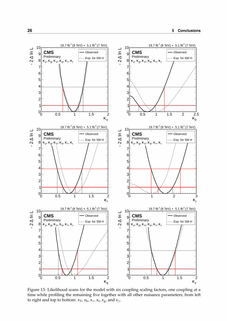
Test of a model with six independent scaling factors We explore a model with six inde-pendent coupling scaling factors by making the following assumptions:

• The couplings to W and Z bosons are scaled by a common factor κV;

• The couplings to third generation fermions, i.e., the top quark, bottom quark, andtau lepton, are scaled independently by κt, κb, and κτ;

• The scale factors for couplings to the first and second generation fermions are equalto those for the third;

• The effective couplings to gluons and photons, induced by loop diagrams, are givenindependent scaling factors κg and κγ, respectively;

• The partial width ΓBSM is zero.

The results of the likelihood scans for these six parameters, one at a time while profiling theremaining five together with all other nuisance parameters, are shown in Fig. 13. The currentdata do not show any statistically significant deviations with respect to the SM Higgs bosonhypothesis. For every κ, the measured 95% CL interval contains unity. A goodness-of-fit testbetween the parameters measured in this model and the SM prediction yields a χ2/(dof) =7.5/6, which corresponds to an asymptotic p-value of 0.28.

Constraints on BRBSM in a scenario with free couplings An alternative, more generalscenario than that with six parameters can be obtained by allowing for a non-vanishing ΓBSM,but constraining κV ≤ 1, a requirement motivated by electroweak symmetry breaking.

Figure 14 shows the likelihood scan versus BRBSM derived in this scenario while profiling allthe other coupling modifiers and nuisance parameters. Within these assumptions, the dataallow us to conclude that BRBSM is in the interval [0.00,0.58] at 95% CL.

Summary of tests of the compatibility of the data with the SM Higgs boson couplingsTable 5 summarizes the tests performed on the compatibility of the data with the expected SMHiggs boson couplings. No statistically significant deviations are observed.

5 ConclusionsProperties of the Higgs boson with mass near 125 GeV are measured in proton-proton collisionswith the CMS experiment at the LHC. A comprehensive set of production and decay measure-ments are combined. The decays to γγ, ZZ, WW, ττ, and bb pairs are exploited, includingstudies targeting Higgs bosons produced in association with a pair of top quarks. The datasamples were collected in 2011 and 2012 and correspond to integrated luminosities of up to5.1 fb−1 at 7 TeV and up to 19.7 fb−1 at 8 TeV; the final detector calibration and alignment areused in the event reconstruction. From the high-resolution γγ and ZZ channels, the mass ofthis Higgs boson is measured to be 125.03 +0.26

−0.27 (stat.) +0.13−0.15 (syst.) GeV, with the precision dom-

inated by the statistical uncertainty. For this mass, the event yields obtained in the differentanalyses tagging specific decay modes and production mechanisms are consistent with thoseexpected for the standard model Higgs boson. The combined best-fit signal strength, relativeto the standard model expectation, is found to be 1.00 ± 0.09 (stat.) +0.08

−0.07 (theo.) ± 0.07 (syst.)at the measured mass. Various searches for deviations in the magnitudes of the Higgs bosonscalar couplings from those predicted for the standard model are performed. No significantdeviations are found.

26 5 Conclusions

Vκ0 0.5 1 1.5 2

ln L

∆-

2

0

1

2

3

4

5

6

7

8

9

10Observed

Exp. for SM H

CMSPreliminary

(7 TeV)-1 (8 TeV) + 5.1 fb-119.7 fb

tκ, τκ, bκ, Vκ, gκ, γκ

bκ0 0.5 1 1.5 2 2.5

ln L

∆-

2

0

1

2

3

4

5

6

7

8

9

10Observed

Exp. for SM H

CMSPreliminary

(7 TeV)-1 (8 TeV) + 5.1 fb-119.7 fb

tκ, τκ, bκ, Vκ, gκ, γκ

τκ0 0.5 1 1.5 2

ln L

∆-

2

0

1

2

3

4

5

6

7

8

9

10Observed

Exp. for SM H

CMSPreliminary

(7 TeV)-1 (8 TeV) + 5.1 fb-119.7 fb

tκ, τκ, bκ, Vκ, gκ, γκ

tκ0 1 2 3

ln L

∆-

2

0

1

2

3

4

5

6

7

8

9

10Observed

Exp. for SM H

CMSPreliminary

(7 TeV)-1 (8 TeV) + 5.1 fb-119.7 fb

tκ, τκ, bκ, Vκ, gκ, γκ

gκ0 0.5 1 1.5 2

ln L

∆-

2

0

1

2

3

4

5

6

7

8

9

10Observed

Exp. for SM H

CMSPreliminary

(7 TeV)-1 (8 TeV) + 5.1 fb-119.7 fb

tκ, τκ, bκ, Vκ, gκ, γκ

γκ0 0.5 1 1.5 2

ln L

∆-

2

0

1

2

3

4

5

6

7

8

9

10Observed

Exp. for SM H

CMSPreliminary

(7 TeV)-1 (8 TeV) + 5.1 fb-119.7 fb

tκ, τκ, bκ, Vκ, gκ, γκ

Figure 13: Likelihood scans for the model with six coupling scaling factors, one coupling at atime while profiling the remaining five together with all other nuisance parameters; from leftto right and top to bottom: κV, κb, κτ, κt, κg, and κγ.

27

Table 5: Tests of the compatibility of the data with the SM Higgs boson couplings. The best-fitvalues and 68% and 95% CL confidence intervals are given for the evaluated scaling factors κior ratios λij = κi/κj. The different compatibility tests discussed in the text are separated byhorizontal lines. When one of the scaling factors in a group is evaluated, others are treated asnuisance parameters.

Model Best-fit resultComment

ParametersTable inRef. [27]

Parameter 68% CL 95% CL

κZ, λWZ (κf =1) - λWZ 0.94+0.22−0.18 [0.61,1.45]

λWZ = κW/κZusing ZZ and0/1-jet WW channels.

κZ, λWZ, κf44

(top)λWZ 0.91+0.14

−0.12 [0.70,1.22] λWZ = κW/κZ fromfull combination.

κV, κf43

(top)κV 1.01+0.07

−0.07 [0.88,1.15] κV scales couplingsto W and Z bosons.

κf 0.89+0.14−0.13 [0.64,1.16] κf scales couplings

to all fermions.

κg, κγ48

(top)κg 0.89+0.10

−0.10 [0.69,1.10] Effective couplings togluons (g) and photons (γ).κγ 1.15+0.13

−0.13 [0.89,1.42]

κg, κγ, BRBSM48

(middle)BRBSM ≤ 0.13 [0.00,0.32] Branching fraction

for BSM decays.

κV, λdu, κu46

(top)λdu 1.01+0.20

−0.19 [0.66,1.43]λdu = κu/κd, relatingup-type and down-typefermions.

κV, λ`q, κq47

(top)λ`q 1.02+0.22

−0.21 [0.61,1.49] λ`q = κ`/κq, relatingleptons and quarks.

κg, κγ, κV,

κb, κτ, κt

Similar to50 (top)

κg 0.76+0.15−0.13 [0.51,1.09]

κγ 0.99+0.18−0.17 [0.66,1.37]

κV 0.97+0.15−0.16 [0.64,1.26]

κb 0.67+0.31−0.32 [0.00,1.31] Down-type quarks (via b).

κτ 0.83+0.19−0.18 [0.48,1.22] Charged leptons (via τ).

κt 1.61+0.33−0.32 [0.97,2.28] Up-type quarks (via t).

as aboveplus BRBSM

and κV ≤ 1- BRBSM ≤ 0.34 [0.00,0.58]

28 References

BSMBR0 0.2 0.4 0.6 0.8 1

ln L

∆-

2

0

1

2

3

4

5

6

7

8

9

10Observed

Exp. for SM H

CMSPreliminary

(7 TeV)-1 (8 TeV) + 5.1 fb-119.7 fb

1,≤Vκ, gκ, γκBSM

, BRtκ, τκ, bκ

Figure 14: The likelihood scan versus BRBSM = ΓBSM/Γtot. The solid curve represents theobservation in data and the dashed curve indicates the expected median results in the presenceof the SM Higgs boson. The modifiers for both the tree-level and loop-induced couplings areprofiled, but the couplings to the electroweak bosons are assumed to be bound by the SMexpectation (κV ≤ 1).

References[1] S. L. Glashow, “Partial-symmetries of weak interactions”, Nucl. Phys. 22 (1961) 579,

doi:10.1016/0029-5582(61)90469-2.

[2] S. Weinberg, “A model of leptons”, Phys. Rev. Lett. 19 (1967) 1264,doi:10.1103/PhysRevLett.19.1264.

[3] A. Salam, “Weak and electromagnetic interactions”, in Elementary particle physics:relativistic groups and analyticity, N. Svartholm, ed., p. 367. Almqvist & Wiskell, 1968.Proceedings of the 8th Nobel symposium.

[4] F. Englert and R. Brout, “Broken symmetry and the mass of gauge vector mesons”, Phys.Rev. Lett. 13 (1964) 321, doi:10.1103/PhysRevLett.13.321.

[5] P. W. Higgs, “Broken symmetries, massless particles and gauge fields”, Phys. Lett. 12(1964) 132, doi:10.1016/0031-9163(64)91136-9.

[6] P. W. Higgs, “Broken symmetries and the masses of gauge bosons”, Phys. Rev. Lett. 13(1964) 508, doi:10.1103/PhysRevLett.13.508.

[7] G. S. Guralnik, C. R. Hagen, and T. W. B. Kibble, “Global conservation laws and masslessparticles”, Phys. Rev. Lett. 13 (1964) 585, doi:10.1103/PhysRevLett.13.585.

[8] P. W. Higgs, “Spontaneous symmetry breakdown without massless bosons”, Phys. Rev.145 (1966) 1156, doi:10.1103/PhysRev.145.1156.

[9] T. W. B. Kibble, “Symmetry breaking in non-Abelian gauge theories”, Phys. Rev. 155(1967) 1554, doi:10.1103/PhysRev.155.1554.

References 29

[10] ATLAS Collaboration, “Observation of a new particle in the search for the standardmodel Higgs boson with the ATLAS detector at the LHC”, Phys. Lett. B 716 (2012) 1,doi:10.1016/j.physletb.2012.08.020, arXiv:1207.7214.

[11] CMS Collaboration, “Observation of a new boson at a mass of 125 GeV with the CMSexperiment at the LHC”, Phys. Lett. B 716 (2012) 30,doi:10.1016/j.physletb.2012.08.021, arXiv:1207.7235.

[12] CMS Collaboration, “Observation of a new boson with mass near 125 GeV in ppcollisions at

√s = 7 and 8 TeV”, JHEP 06 (2013) 081,

doi:10.1007/JHEP06(2013)081, arXiv:1303.4571.

[13] ATLAS Collaboration, “Measurement of the Higgs boson mass from the H → γγ andH → ZZ∗ → 4` channels with the ATLAS detector using 25 fb−1 of pp collision data”,(2014). arXiv:1406.3827. Submitted for publication in Phys. Rev. D.

[14] CMS Collaboration, “Search for the standard model Higgs boson produced in associationwith a top-quark pair in pp collisions at the LHC”, JHEP 05 (2013) 145,doi:10.1007/JHEP05(2013)145, arXiv:1303.0763.

[15] ATLAS Collaboration, “Measurements of Higgs boson production and couplings indiboson final states with the ATLAS detector at the LHC”, Phys. Lett. B 726 (2013) 88,doi:10.1016/j.physletb.2013.08.010, arXiv:1307.1427.

[16] CMS Collaboration, “Search for the standard model Higgs boson produced in associationwith a W or a Z boson and decaying to bottom quarks”, Phys. Rev. D 89 (2014) 012003,doi:10.1103/PhysRevD.89.012003, arXiv:1310.3687.

[17] CMS Collaboration, “Measurement of Higgs boson production and properties in the WWdecay channel with leptonic final states”, JHEP 01 (2014) 096,doi:10.1007/JHEP01(2014)096, arXiv:1312.1129.

[18] CMS Collaboration, “Measurement of the properties of a Higgs boson in the four-leptonfinal state”, Phys. Rev. D 89 (2014) 092007, doi:10.1103/PhysRevD.89.092007,arXiv:1312.5353.

[19] CMS Collaboration, “Evidence for the 125 GeV Higgs boson decaying to a pair of τleptons”, JHEP 05 (2014) 104, doi:10.1007/JHEP05(2014)104,arXiv:1401.5041.

[20] CMS Collaboration, “Observation of the diphoton decay of the 125 GeV Higgs bosonand measurement of its properties”, CMS-HIG-13-001, CERN-PH-EP-2014-117, 2014.Submitted for publication in Eur. Phys. J. C.

[21] CMS Collaboration, “Search for a Higgs boson decaying into a Z and a photon in ppcollisions at

√s = 7 and 8 TeV”, Phys. Lett. B 726 (2013) 587,

doi:10.1016/j.physletb.2013.09.057, arXiv:1307.5515.

[22] ATLAS Collaboration, “Search for Higgs boson decays to a photon and a Z boson in ppcollisions at

√s = 7 and 8 TeV with the ATLAS detector”, Phys. Lett. B 732 (2014) 8,

doi:10.1016/j.physletb.2014.03.015, arXiv:1402.3051.

[23] ATLAS Collaboration, “Search for Invisible Decays of a Higgs Boson Produced inAssociation with a Z Boson in ATLAS”, Phys. Rev. Lett. 112 (2014) 201802,doi:10.1103/PhysRevLett.112.201802, arXiv:1402.3244.

30 References

[24] CMS Collaboration, “Search for invisible decays of Higgs bosons in the vector bosonfusion and associated ZH production modes”, (2014). arXiv:1404.1344. Submittedfor publication in Eur. Phys. J. C.

[25] CMS Collaboration, “Study of the mass and spin-parity of the Higgs boson candidate viaits decays to Z boson pairs”, Phys. Rev. Lett. 110 (2013) 081803,doi:10.1103/PhysRevLett.110.081803, arXiv:1212.6639.

[26] ATLAS Collaboration, “Evidence for the spin-0 nature of the Higgs boson using ATLASdata”, Phys. Lett. B 726 (2013) 120, doi:10.1016/j.physletb.2013.08.026,arXiv:1307.1432.

[27] LHC Higgs Cross Section Working Group, “Handbook of LHC Higgs Cross Sections: 3.Higgs Properties”, (2013). arXiv:1307.1347.

[28] CMS Collaboration, “Search for Higgs Boson Production in Association with aTop-Quark Pair and Decaying to Bottom Quarks or Tau Leptons”, Technical ReportCMS-PAS-HIG-13-019, CERN, Geneva, 2013.

[29] CMS Collaboration, “Search for the standard model Higgs boson produced in associationwith top quarks in multilepton final states”, Technical Report CMS-PAS-HIG-13-020,CERN, Geneva, 2013.

[30] CMS Collaboration, “Evidence for the direct decay of the 125 GeV Higgs boson tofermions”, Nat. Phys. advance online publication (2014) doi:10.1038/nphys3005,arXiv:1401.6527.

[31] CMS Collaboration, “The CMS experiment at the CERN LHC”, JINST 3 (2008) S08004,doi:10.1088/1748-0221/3/08/S08004.

[32] ATLAS and CMS Collaborations, LHC Higgs Combination Group, “Procedure for theLHC Higgs boson search combination in Summer 2011”, Technical ReportATL-PHYS-PUB 2011-11, CMS NOTE 2011/005, 2011.

[33] CMS Collaboration, “Combined results of searches for the standard model Higgs bosonin pp collisions at

√s = 7 TeV”, Phys. Lett. B 710 (2012) 26,

doi:10.1016/j.physletb.2012.02.064, arXiv:1202.1488.

[34] G. Cowan, K. Cranmer, E. Gross, and O. Vitells, “Asymptotic formulae forlikelihood-based tests of new physics”, Eur. Phys. J. C 71 (2011) 1554,doi:10.1140/epjc/s10052-011-1554-0, arXiv:1007.1727.

[35] L. Moneta et al., “The RooStats Project”, in 13th International Workshop on AdvancedComputing and Analysis Techniques in Physics Research (ACAT2010). SISSA, 2010.arXiv:1009.1003. PoS(ACAT2010)057.

[36] B. Efron, “Bootstrap methods: another look at the jackknife”, Ann. Statist. 7 (1979) 1,doi:10.1214/aos/1176344552. See “Remark K”.

[37] S. M. S. Lee and G. A. Young, “Parametric bootstrapping with nuisance parameters”,Statist. Probab. Lett. 71 (2005) 143, doi:10.1016/j.spl.2004.10.026.

[38] L. D. Landau, “On the angular momentum of a two-photon system”, Dokl. Akad. Nauk60 (1948) 207.

References 31

[39] C. N. Yang, “Selection rules for the dematerialization of a particle into two photons”,Phys. Rev. 77 (1950) 242, doi:10.1103/PhysRev.77.242.

[40] M. J. G. Veltman, “Limit on mass differences in the Weinberg model”, Nucl. Phys. B 123(1977) 89, doi:10.1016/0550-3213(77)90342-X.

[41] P. Sikivie, L. Susskind, M. B. Voloshin, and V. I. Zakharov, “Isospin breaking intechnicolor models”, Nucl. Phys. B 173 (1980) 189,doi:10.1016/0550-3213(80)90214-X.