CMSC 451: Network Flows

Slides By: Carl Kingsford

Department of Computer Science

University of Maryland, College Park

Based on Sections 7.1&7.2 of Algorithm Design by Kleinberg & Tardos.

Network Flows

• Our 4th major algorithm design technique(greedy, divide-and-conquer, and dynamic programming arethe others).

• A little different than the others: we’ll see an algorithm forone problem (and minor variants) that is so useful that wecan apply to to many practical problems.

• Called network flow.

Network flow problem, e.g.

10 5

2

3

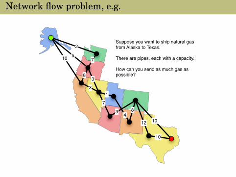
Suppose you want to ship natural gas from Alaska to Texas.

There are pipes, each with a capacity.

How can you send as much gas as possible?

3

7

8

7

1

3 48

1012

10

Flow Network

A flow network is a connected, directed graph G = (V , E ).

• Each edge e has a non-negative, integer capacity ce .

• A single source s ∈ V .

• A single sink t ∈ V .

• No edge enters the source and no edge leaves the sink.

s

u

v

t

x

w

20

10

3010

10

30

10

20

Assumptions

To repeat, we make these assumptions about the network:

1 Capacities are integers.

2 Every node has one edge adjacent to it.

3 No edge enters the source and no edge leaves the sink.

These assumptions can all be removed.

Flow

Def. An s-t flow is a function f : E → R≥0 that assigns a realnumber to each edge.

Intuitively, f (e) is the amount of material carried on the edge e.

s

u

v

t

x

w

20

10

3020

5

30

10

20

10

10

5

15

15

5

10

Flow constraints

Constraints on f :

1 0 ≤ f (e) ≤ ce for each edge e. (capacity constraints)

2 For each node v except s and t, we have:∑e into v

f (e) =∑

e leaving v

f (e) .

(balance constraints: whatever flows in, must flow out).

v

10

3

2

7

4

Notation

The value of flow f is:

v(f ) =∑

e out of s

f (e)

This is the amount of material that s is able to send out.

Notation:

• f in(v) =∑

e into v f (e)

• f out(v) =∑

e leaving v f (e)

Balance constraints becomes: f in(v) = f out(v) for all v 6∈ {s, t}

Maximum Flow Problem

Definition (Value)

The value v(f ) of a flow f is f out(s).

That is: it is the amount of material that leaves s.

Maximum Flow Problem

Given a flow network G , find a flow f of maximum possible value.

A Greedy Start

A Greedy Start:

1 Suppose we let f (e) = 0 for all edges (no flow anywhere).

2 Choose some s − t path and “push” flow along it up to thecapacities. Repeat.

3 When we get stuck, we can erase some flow along certainedges.

How do we make this more precise?

Example

s

u

v

t

20 / 20

10

20 / 30

20 / 20

10

After 1 path, we've allocated 20 units

s

u

v

t

20 / 20

10

20 / 30

20 / 20

10

Want to send the blue path

10

Residual Graph

We define a residual graph Gf . Gf depends on some flow f :

1 Gf contains the same nodes as G .

2 Forward edges: For each edge e = (u, v) of G for whichf (e) < ce , include an edge e ′ = (u, v) in Gf with capacityce − f (e).

3 Backward edges: For each edge e = (u, v) in G withf (e) > 0, we include an edge e ′ = (v , u) in Gf with capacityf (e).

Residual Graph, e.g.

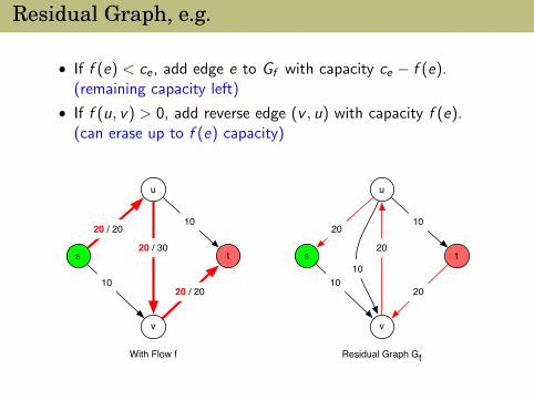
• If f (e) < ce , add edge e to Gf with capacity ce − f (e).(remaining capacity left)

• If f (u, v) > 0, add reverse edge (v , u) with capacity f (e).(can erase up to f (e) capacity)

s

u

v

t

20 / 20

10

20 / 30

20 / 20

10

With Flow f

s

u

v

t

20

10

20

20

10

Residual Graph Gf

10

Augmenting Paths

• Let P be an s − t path in the residual graph Gf .

• Let bottleneck(P, f ) be the smallest capacity in Gf on anyedge of P.

• If bottleneck(P, f ) > 0 then we can increase the flow bysending bottleneck(P, f ) along the path P.

Augmenting Paths, 2

If bottleneck(P, f ) > 0 then we can increase the flow by sendingbottleneck(P, f ) along the path P:

augment(f, P):b = bottleneck(P,f)For each edge (u,v) ∈ P:

If e = (u,v) is a forward edge:Increase f(e) in G by b //add some flow

Else:e’ = (v,u)Decrease f(e’) in G by b //erase some flow

EndIfEndForReturn f

Ford-Fulkerson Algorithm

MaxFlow(G):// initialize:Set f[e] = 0 for all e in G

// while there is an s-t path in Gf:While P = FindPath(s,t, Residual(G,f)) != None:

f = augment(f, P)UpdateResidual(G, f)

EndWhileReturn f

After augment, we still have a flow

After f ′ = augment(P, f ), we still have a flow:

Capacity constraints: Let e be an edge on P:

• if e is forward edge, it has capacity ce − f (e). Therefore,

f ′(e) = f (e) + bottleneck(P, f ) ≤ f (e) + ce − f (e) ≤ ce

• if e is a backward edge, it has capacity f (e). Therefore,

f ′(e) = f (e)− bottleneck(P, f ) ≥ f (e)− f (e) = 0

Still have flow, 2

Balance constraints: An s-t path in Gf corresponds to some setof edges in G :

s t+b +b -b -b +b

In other pictures,

v

10

3 + bottleneck(P,f)

7 + bottleneck(P,f)6

v

10 - bottleneck(P,f)

3 + bottleneck(P,f)

6

7

Running Time

1 At every step, the flow values f (e) are integers.

Start withints and always add or subtract ints

2 At every step we increase the amount of flow v(f ) sent by atleast 1 unit.

3 We can never send more than C :=∑

e leaving s ce .

Theorem

The Ford-Fulkerson algorithm terminates in C iterations of theWhile loop.

Running Time

1 At every step, the flow values f (e) are integers. Start withints and always add or subtract ints

2 At every step we increase the amount of flow v(f ) sent by atleast 1 unit.

3 We can never send more than C :=∑

e leaving s ce .

Theorem

The Ford-Fulkerson algorithm terminates in C iterations of theWhile loop.

Time in the While loop

1 If G has m edges, Gf has ≤ 2m edges.

2 Can find an s − t path in Gf in time O(m + n) time with DFSor BFS.

3 Since m ≥ n/2 (every node is adjacent to some edge),O(m + n) = O(m).

Theorem

The Ford-Fulkerson algorithm runs in O(mC ) time.

Caveats, etc.

Note this is pseudo-polynomial because it depends on the size ofthe integers in the input.

You can remove this with slightly different algorithms. E.g.:

• O(nm2): Edmonds-Karp algorithm (use BFS to find theaugmenting path)

• O(m2 log C ) (see section 7.3), or

• O(n2m) or O(n3) (see section 7.4).

Proof of correctness

How do we know the flow ismaximum?

Cuts and Cut Capacity

s

t

AB = V \ A

s-t cut

10

2

3

12

9

capacity(A,B) = 25

Definition

The capacity(A, B) of an s-t cut (A, B) is the sum of thecapacities of edges leaving A.

A Cut Theorem

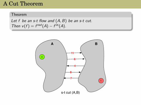
Theorem

Let f be an s-t flow and (A, B) be an s-t cut.Then v(f ) = f out(A)− f in(A).

s

t

A B

s-t cut (A,B)

11

6

4

8

7

Another cut theorem

Theorem

Let f be any s-t flow and (A, B) be any s-t cut.Then v(f ) ≤ capacity(A, B).

Proof.

v(f ) = f out(A)− f in(A) prev. thm

≤ f out(A) f in(A) is ≥ 0

=∑

e leaving A

f (e) by definition

≤∑

e leaving A

ce by capacity constraints

= capacity(A, B) by definition

Cuts Constrain Flows

This theorem:

Theorem

Let f be any s-t flow and (A, B) be any s-t cut.Then v(f ) ≤ capacity(A, B).

Says that any cut is bigger than any flow.

Therefore, cuts constrain flows. The minimum capacity cutconstrains the maximum flow the most.

In fact, the capacity of the minimum cut always equals themaximum flow value.

Max-Flow = Min-Cut

capacities of cuts

values of flows

minimum capacity of a cut = maximum value of a flow

Max-Flow = Min-Cut, 2

Let f ∗ be the flow returned by our algorithm.Look at Gf ∗ but define a cut in G :

s

t

Cut = (A*, B*)

A* = nodes reachable from s in residual graph Gf*

Blue edges must be saturated.Red edges must have 0 flow =⇒ v(f ∗) = capacity(A∗, B∗).

Max-Flow = Min-Cut, 3

s

t

Cut = (A*, B*)

A* = nodes reachable from s in residual graph Gf*

X

X

• (A∗, B∗) is an s-t cut because there is no path from s to t inthe residual graph Gf ∗ .

• Edges (u, v) from A∗ to B∗ must be saturated — otherwisethere would be a forward edge (u, v) in Gf ∗ and v would bepart of A∗.

• Edges (v , u) from B∗ to A∗ must be empty — otherwise therewould be a backedge (u, v) in Gf ∗ and v would be part of A∗.

Max-Flow = Min-Cut, 4

Therefore,

• v(f ∗) = capacity(A∗, B∗).

• No flow can have value bigger than capacity(A∗, B∗).

• So, f ∗ must be an maximum flow.

• And (A∗, B∗) has to be a minimum-capacity cut.

Theorem (Max-flow = Min-cut)

The value of the maximum flow in any flow graph is equal to thecapacity of the minimum cut.

Finding the Min-capacity Cut

Our proof that maximum flow = minimum cut can be used toactually find the minimum capacity cut:

1 Find the maximum flow f ∗.

2 Construct the residual graph Gf ∗ for f ∗.

3 Do a BFS to find the nodes reachable from s in Gf ∗ . Let theset of these nodes be called A∗.

4 Let B∗ be all other nodes.

5 Return (A∗, B∗) as the minimum capacity cut.

To Summarize

Summary:

• Ford-Fulkerson algorithm can find max flow in O(mC ) time.

• Algorithm idea: Send flow along some path with capacityleft, possibly “erasing” some flow we’ve already sent. Useresidual graph to keep track of remaining capacities and flowwe’ve already sent.

• We can eliminate C to get a true polynomial algorithm byusing BFS to find our augmenting paths.

• All cuts have capacity ≥ the value of all flows.

• Know the flow is maximum because its value equals thecapacity of some cut.